SEMICLASSICAL WKB PROBLEM FOR THE NON-SELF-ADJOINT DIRAC OPERATOR WITH A DECAYING POTENTIAL

Abstract.

In this paper we examine the semiclassical behavior of the scattering data of a non-self-adjoint Dirac operator with a fairly smooth -but not necessarily analytic- potential decaying at infinity. In particular, using ideas and methods going back to Langer and Olver, we provide a rigorous semiclassical analysis of the scattering coefficients, the Bohr-Sommerfeld condition for the location of the eigenvalues and their corresponding norming constants. Our analysis is motivated by the potential applications to the focusing cubic NLS equation, in view of the well-known fact discovered by Zakharov and Shabat that the spectral analysis of the Dirac operator is the basis of the solution of the NLS equation via inverse scattering theory. This paper complements and extends a previous work of Fujiié and the second author, which considered a more restricted problem for a strictly analytic potential.

1. Introduction

Consider the initial value problem (IVP) of the one-dimensional focusing nonlinear Schrödinger equation (focusing NLS) for the complex field $u(x,t)$, i.e.

$$\begin{cases}i\hbar\partial_{t}u+\frac{\hbar^{2}}{2}\partial_{x}^{2}u+|u|^{2}u=0,\quad(x,t)\in{\mathbb{R}}\times{\mathbb{R}}\\ \ u(x,0)=A(x),\quad x\in{\mathbb{R}}\end{cases}$$ (1.1)

for a real valued function $A$ and a fixed positive number $\hbar$.

Zakharov and Shabat in [22] have proved back in 1972 that the focusing NLS equation is integrable via the Inverse Scattering Transform (IST). A crucial step of the method is the analysis of the following Zakharov-Shabat (or Dirac) eigenvalue problem

$$\hbar\begin{bmatrix}v_{1}^{\prime}(x,\lambda,\hbar)\\ v_{2}^{\prime}(x,\lambda,\hbar)\end{bmatrix}=\begin{bmatrix}-i\lambda&A(x)\\ -A(x)&i\lambda\end{bmatrix}\begin{bmatrix}v_{1}(x,\lambda,\hbar)\\ v_{2}(x,\lambda,\hbar)\end{bmatrix}$$ (1.2)

where $\lambda\in{\mathbb{C}}$ is a “spectral parameter”; here prime denotes differentiation with respect to $x$.

Now let us suppose that $\hbar$ is small compared to the $x,t$ we are interested in. The question raised is then: what is the behavior of solutions of the IVP (1.1) as $\hbar\downarrow 0$? The rigorous analysis of this problem was initiated in [9]. Because of the work of Zakharov and Shabat, the first step in the study of this IVP in the semiclassical limit $\hbar\downarrow 0$ has to be the asymptotic spectral analysis of the scattering problem (1.2) as $\hbar\downarrow 0$, keeping the function $A$ fixed.

The eigenvalue (EV) problem (1.2) is not and cannot be written as an EV problem for a self-adjoint operator. What we study here is a semiclassical WKB problem (or LG problem) for the corresponding non-self-adjoint Dirac operator with potential $A$.

The question of the semiclassical approximation of the scattering data has a deep significance in view of the instability of the NLS problem which appears in many levels. In fact even away from the semiclassical regime, the focusing NLS is the main model for the so-called modulational instability (as in [3]), although for positive fixed $\hbar$ the initial value problem is well-posed.

Semiclassically the instabilities become more pronounced. One way to see this, is related to the underlying ellipticity of the formal semiclassical limit. To be more specific, consider the well-known Madelung transformation

$$\begin{cases}\boldsymbol{\rho}=|u|^{2}\\ \boldsymbol{\mu}=\hbar\Im\,(u^{*}u_{x})\end{cases}$$

where $u^{*}$ denotes the complex conjugate of $u$. Then the IVP (1.1) becomes

$$\begin{cases}\boldsymbol{\rho}_{t}+\boldsymbol{\mu}_{x}=0\\ \boldsymbol{\mu}_{t}+\Big{(}\frac{\boldsymbol{\mu}^{2}}{\boldsymbol{\rho}}+\frac{\boldsymbol{\rho}^{2}}{2}\Big{)}_{x}=\par\frac{\hbar^{2}}{4}\partial_{x}[\boldsymbol{\rho}(\log\boldsymbol{\rho})_{xx}]\end{cases}$$

with initial data $\boldsymbol{\rho}(x,0)=|u|^{2}(x,0)=A^{2}(x)$ and $\boldsymbol{\mu}(x,0)=0$.

The formal limit as $\hbar\downarrow 0$ is

$$\begin{cases}\boldsymbol{\rho}_{t}+\boldsymbol{\mu}_{x}=0\\ \boldsymbol{\mu}_{t}+\Big{(}\frac{\boldsymbol{\mu}^{2}}{\boldsymbol{\rho}}+\frac{\boldsymbol{\rho}^{2}}{2}\Big{)}_{x}=0\end{cases}$$

with initial data $\boldsymbol{\rho}(x,0)=|u|^{2}(x,0)=A^{2}(x)$ and $\boldsymbol{\mu}(x,0)=0$. This is an IVP for an elliptic system of equations and so one expects that small perturbations of the initial data (independent of $\hbar$) can lead to large changes in the solution, at any given time.

Instabilities appear also at different stages of the analysis: the spectral analysis of the related non-self-adjoint Dirac operator, the related equilibrium measure problem (see [10]), the related Whitham equations (cf. [9]) which are also elliptic, the possibility of the appearance of rogue waves (see [2]) and even the numerical studies of the problem (as in [15]).

The semiclassical approximation of the scattering data results in small changes of the initial data; changes $that~{}depend~{}on~{}\hbar$. It is a priori unclear whether these small changes can have a significant effect in the semiclassical asymptotics of the solution of the IVP (1.1) as $\hbar\downarrow 0$. Our ultimate aim is to provide a proof that they do not.

Our work complements the paper [5] of S. Fujiié and the second author where the potential is considered to be a real analytic bell-shaped function and in which the so-called exact WKB method (cf. [4], [6], [7] and [19]) is employed. In this work, we instead suppose that the bell-shaped potential function $A$ has only some prescribed smoothness which we specify explicitly in §2. Our methods are necessarily different since the exact WKB method requires analyticity. Our ideas are rather influenced by the papers [20] and [21] of D. R. Yafaev where an analogous problem is treated for the self-adjoint Schrödinger operator, which in turn rely on works [16] and [17] of F. W. J. Olver . More precisely, Yafaev uses results mainly from [17] while we rely heavily on [16] as well.

The present paper is arranged as follows. In section §2 we state all the necessary assumptions on the potential function $A$ so that Olver’s work can be applied in our case. In section §3 we introduce a simple transformation that maps the Dirac problem to an equivalent Schrödinger problem. Sections §4 and §5 show how the Liouville transformation changes our Schrödinger equation into one containing an error term which is a continuous function on the Liouville plane. By controlling this error term in section §6 we obtain approximate solutions expressed with the help of Parabolic Cylinder Functions (PCFs) in a Liouville variable $\zeta\geq 0$.

In section §7 we illustrate the previously mentioned results for the special case where the potential function is $x\mapsto\frac{1}{1+x^{2}}$. Then in §8 we find the asymptotic behavior of the approximants introduced in §6. In §9 we present some connection formulas that relate the approximate solutions for $\zeta\geq 0$ to the ones for $\zeta\leq 0$. The significance of this connection becomes clear in §10 where we find Bohr-Sommerfeld quantization conditions for the EVs of our problem, uniformly away from zero.

Next in §11 we study the EVs that lie closer to zero and we are able to arrive at uniform bounds all the way to zero. We only do this here for two specific (but quite inclusive) families of functions $A$. It may be that more general conditions can alternatively be posed instead; conditions that would ensure the same results for a wide class of data. But we are not able to do this at this point. Our situation is somewhat comparable to [5] where extra (general but complicated) conditions had to be added, in order to assure a good behavior of the EVs near $0$. Here however, the formula (11.3) we have for the function $\psi$, makes it very easy to check if indeed the behavior of the EVs near zero, is good enough for any family of potentials $A$ defined by explicitly prescribed asymptotics at infinity.

Section §12 is concerned with the amplitudes of the transmission and reflection coefficients (both away and close to zero). Unlike [5], we do not need any extra conditions on $A$ to control the reflection coefficient (cf. §12) near $0$ (even though our estimates are somewhat weaker, they are still good enough for applications). Finally, we make some concluding remarks in section §13.

For the sake of the reader, as the approximate solutions to our problems involve Airy and Parabolic Cylinder Functions, we present all the necessary results concerning these functions in sections A and B of the appendix. There, the reader can also find a section (section C) on a theorem concerning integral equations which is the primary tool in the proof of the main Theorem 6.3.

Notationwise, a bar over a letter (or number) does not denote complex conjugation. For complex conjugation we have reserved the superscript $*$; i.e. $z^{*}$ (and not $\bar{z}$) is the complex conjugate of $z$. The letter $C$ denotes generically a positive constant (appearing in estimates) and $\mathbb{R}_{+}$, $\mathbb{R}_{-}$ represent the sets of positive and negative numbers respectively. Also, we denote the Wronskian of two functions $f$, $g$ by $\mathcal{W}[f,g]$. Furthermore, we write $f\sim g$ when $\tfrac{f}{g}$ tends to $1$. Finally, the notation $f^{2}(x)$ denotes the square of the value of the function $f$ at $x$. Hence, the symbols $f^{2}(x)$ and $f(x)^{2}$ are used interchangeably and are not to be confused with the composition $f\circ f$ of $f$ with itself.

2. The Potential

In this section we state precise assumptions on the potential function $A$ which are sufficient to ensure that all the techniques and methods developed in the following sections can go through easily. In short, we consider bell-shaped functions with some smoothness. To be more precise, we assume the following.

Assumption 2.1.

The function $A$ satisfies

• $A(x)>0$ for $x\in\mathbb{R}$

• $A(-x)=A(x)$ for $x\in\mathbb{R}$

• $A$ is in $C^{4}({\mathbb{R}})$ and of class $C^{5}$ in a neighborhood of $0$

• $xA^{\prime}(x)<0$ for $x\in\mathbb{R}\setminus\{0\}$

• $A^{\prime\prime}(0)<0$; we set $0<A(0)=:A_{max}$

• there exists $\tau>0$ so that

  $$A(x)=\mathcal{O}\Big{(}\tfrac{1}{|x|^{1+\tau}}\Big{)}\quad\text{as}\quad x\to\pm\infty$$

  $$A^{\prime}(x)=\mathcal{O}\Big{(}\tfrac{1}{|x|^{2+\tau}}\Big{)}\quad\text{as}\quad x\to\pm\infty$$

  $$A^{\prime\prime}(x)=\mathcal{O}\Big{(}\tfrac{1}{|x|^{3+\tau}}\Big{)}\quad\text{as}\quad x\to\pm\infty.$$

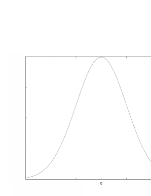
Figure 1. A bell-shaped function.

Now let $\mu\in(0,A_{max}]\subset\mathbb{R}_{+}$. Observe that

• for $\mu\in(0,A_{max})$ the equation $A(x)=\mu$ has exactly two solutions $x_{\pm}$ which of course depend on $\mu$ and by the symmetry of $A$ satisfy $x_{\mp}=-x_{\pm}$. Furthermore, $A(x)>\mu$ for $x\in(x_{-},x_{+})$ and $A(x)<\mu$ for $x\in(-\infty,x_{-})\cup(x_{+},+\infty)$.

• when $\mu=A_{max}$ the two points $x_{\pm}$ coalesce into one double at $x=0$.

We believe that neither the evenness assumption, nor the single local maximum assumption are strictly necessary. If evenness is not imposed, we have what Klaus & Shaw call a “single lobe” potential (see [11] and [12]). Essentially our discussion in this article goes through mostly unaltered, since the results of Klaus & Shaw mentioned below (in §3) are still valid. One thing that changes is that the norming constants are no more real, but we still have uniform estimates for them (see Corollary 10.5). If the single local maximum assumption is dropped we no more expect to have imaginary EVs. But we do expect to have EVs accumulate along curves as in sections §10, §11 and Bohr-Sommerfeld conditions to appear. A forthcoming paper will hopefully show how to handle more general cases.

3. From Dirac to Schrödinger

As stated in the introduction, in this paper we examine the scattering data for a Dirac operator. We start with an investigation of the EVs. Specifically, we study the EV problem

$$\mathfrak{D}_{\hbar}\mathbf{u}=\lambda\mathbf{u}$$ (3.1)

where $\mathfrak{D}_{\hbar}$ is the Dirac operator

$$\mathfrak{D}_{\hbar}:=\begin{bmatrix}i\hbar\partial_{x}&-iA\\ -iA&-i\hbar\partial_{x}\end{bmatrix}$$ (3.2)

with $0<\hbar\ll 1$ a small parameter (Planck), $A$ as in §2 and $\mathbf{u}=[u_{1}\hskip 3.0ptu_{2}]^{T}$ is a function from $\mathbb{R}$ to $\mathbb{C}^{2}$. As usual, $\lambda\in{\mathbb{C}}$ plays the role of the spectral parameter.

Let us make explicit what we mean when we discuss about the EVs of the operator in (3.2). We have the following definition.

Definition 3.1.

A number $\lambda\in\mathbb{C}$ is an eigenvalue of the operator $\mathfrak{D}_{\hbar}$ if equation (3.1) has a non-trivial solution $\mathbf{u}\in L^{2}(\mathbb{R};\mathbb{C}^{2})$; that is

$$0<\int_{-\infty}^{+\infty}\Big{[}|u_{1}(x)|^{2}+|u_{2}(x)|^{2}\Big{]}dx<+\infty.$$

The spectral characteristics of an operator like $\mathfrak{D}_{\hbar}$ having a potential $A$ satisfying the assumptions of §2 have been established in [11] and [12] by M. Klaus and J. K. Shaw. More precicely we know that

• the continuous spectrum of $\mathfrak{D}_{\hbar}$ is the whole real line $\mathbb{R}$ and

• the EVs are simple, purely imaginary and symmetric with respect to the real axis; their imaginary part lying in $[-A_{max},A_{max}]$

The spectral facts above suggest writing $\lambda=i\mu$ for $0<\mu\leq A_{max}$ (due to symmetry). Hence, (3.1) is written as

$$\hbar\begin{bmatrix}u_{1}^{\prime}(x,\mu,\hbar)\\ u_{2}^{\prime}(x,\mu,\hbar)\end{bmatrix}=\begin{bmatrix}\mu&A(x)\\ -A(x)&-\mu\end{bmatrix}\begin{bmatrix}u_{1}(x,\mu,\hbar)\\ u_{2}(x,\mu,\hbar)\end{bmatrix}$$ (3.3)

where the prime denotes differentiation with respect to $x$.

Under the change of variables (cf. equation (4) in [14])

$$y_{\pm}=\frac{u_{2}\pm u_{1}}{\sqrt{A\mp\mu}}$$ (3.4)

system (3.3) is equivalent to the following two independent equations

$$y_{\pm}^{\prime\prime}=\bigg{\{}\hbar^{-2}[\mu^{2}-A^{2}(x)]+\frac{3}{4}\Big{[}\frac{A^{\prime}(x)}{A(x)\mp\mu}\Big{]}^{2}-\frac{1}{2}\frac{A^{\prime\prime}(x)}{A(x)\mp\mu}\bigg{\}}y_{\pm}$$ (3.5)

where we dropped the dependence of $y_{\pm}$ on $(x,\mu,\hbar)$ for notational simplicity. Again, prime denotes differentiation with respect to $x$.

In (3.5), we will only consider the equation with the lower index because the term

$$\frac{3}{4}\Big{[}\frac{A^{\prime}(x)}{A(x)+\mu}\Big{]}^{2}-\frac{1}{2}\frac{A^{\prime\prime}(x)}{A(x)+\mu}$$

has no singularities and thus work with the equation

$$\frac{d^{2}y}{dx^{2}}=\bigg{\{}\hbar^{-2}[\mu^{2}-A^{2}(x)]+\frac{3}{4}\Big{[}\frac{A^{\prime}(x)}{A(x)+\mu}\Big{]}^{2}-\frac{1}{2}\frac{A^{\prime\prime}(x)}{A(x)+\mu}\bigg{\}}y.$$ (3.6)

Observe that the change of variables (3.4) with the minus choice does not alter the discrete spectrum. Hence we are led to the following important fact.

Proposition 3.2.

Finding the discrete spectrum of $\mathfrak{D}_{\hbar}$ in (3.2) is equivalent to finding the values of $\mu\in(0,A_{max}]$ for which (3.6) has an $L^{2}(\mathbb{R})$ solution.

Now, let us choose any $A_{0}$ such that $0<A_{0}<A_{max}$. In equation (3.6) $x$ runs on the whole real line ${\mathbb{R}}$ and $\mu$ will play the role of a spectral parameter in $[A_{0},A_{max}]\subset{\mathbb{R}}_{+}$. For $\mu\in[A_{0},A_{max})$ the function $x\mapsto\mu^{2}-A^{2}(x)$ is non-vanishing on ${\mathbb{R}}$ except for two distinct simple zeros at $x=x_{-}$ and $x=x_{+}$ with $x_{-}<x_{+}$. In the critical case $\mu=A_{max}$ the function $x\mapsto A_{max}^{2}-A^{2}(x)$ has a single double zero at $x=0$. Both $x_{-}$, $x_{+}$ are continuous functions of the parameter $\mu$ and tend to zero as $\mu\uparrow A_{max}$.

Figure 2. The relationship between parameters $\mu$ and $a$.

We introduce a change of variables for the spectral parameter $\mu$ in order to rely on the results from [16]. For this, we first define the function $B$ to be the restriction of $A$ on $[0,+\infty)$, i.e. $B={\left.\kern-1.2ptA\vphantom{\big{|}}\right|_{[0,+\infty)}}$ and note that, by the assumptions on $A$, the function $B$ is invertible. We set

$$a=x_{+}$$

so

$$A(x_{+})=\mu\Leftrightarrow B(a)=\mu\Leftrightarrow a=B^{-1}(\mu).$$

Since $B$ is a decreasing function, so is $B^{-1}$ and we get

$$a\in B^{-1}\Big{(}[A_{0},A_{max}]\Big{)}=[0,B^{-1}(A_{0})]=:[0,a_{0}].$$

Thus, the zeros of $x\mapsto A^{2}(a)-A^{2}(x)$ are located at $x_{\pm}=\pm a$. Furthermore, the critical value of $a$ is now zero and $a$ ranges over the compact interval $[0,a_{0}]$ (we should add that $A_{0}$ and consequently $a_{0}$ may be allowed to depend on $\hbar$ as is the case in §11).

With this new parameter, equation (3.6) is replaced by

$$\frac{d^{2}y}{dx^{2}}=[\hbar^{-2}f(x,a)+g(x,a)]y$$ (3.7)

where $f$ and $g$ satisfy

$$f(x,a)=A^{2}(a)-A^{2}(x)$$ (3.8)

and

$$g(x,a)=\frac{3}{4}\Big{[}\frac{A^{\prime}(x)}{A(x)+A(a)}\Big{]}^{2}-\frac{1}{2}\frac{A^{\prime\prime}(x)}{A(x)+A(a)}.$$ (3.9)

We close this section with an important definition concerning the zeros of $f$ in (3.8).

Definition 3.3.

The zeros (with respect to $x$) of the function

$$f(x,a)=A^{2}(a)-A^{2}(x)$$

are called turning ponts (or transition points) of the equation (3.7).

Hence our equation facilitates two turning points at $x=\pm a$.

4. The Liouville Transformation

In this section we introduce new variables $Y$ and $\zeta$ according to the Liouville transform

$$Y=\dot{x}^{-\frac{1}{2}}y$$

where the dot signifies differentiation with respect to $\zeta$. Equation (3.7) becomes

$$\frac{d^{2}Y}{d\zeta^{2}}=\Big{[}\hbar^{-2}\dot{x}^{2}f(x,a)+\dot{x}^{2}g(x,a)+\dot{x}^{\frac{1}{2}}\frac{d^{2}}{d\zeta^{2}}(\dot{x}^{-\frac{1}{2}})\Big{]}Y.$$ (4.1)

In our case, $f(\cdot,a)$ is negative in $(-a,a)$ and positive in $(-\infty,-a)\cup(a,+\infty)$. Hence we prescribe

$$\dot{x}^{2}f(x,a)=\zeta^{2}-\alpha^{2}$$ (4.2)

where $\alpha\geq 0$ is chosen in such a way that $x=-a$ corresponds to $\zeta=-\alpha$ and $x=a$ to $\zeta=\alpha$ accordingly. Indeed, after integration, (4.2) yields

$$\int_{-a}^{x}[-f(t,a)]^{\frac{1}{2}}dt=\int_{-\alpha}^{\zeta}(\alpha^{2}-\tau^{2})^{\frac{1}{2}}d\tau$$ (4.3)

provided that $-a\leq x\leq a$. Notice that by taking these integration limits, $-a$ corresponds to $-\alpha$. For the remaining correspondence, we require

$$\int_{-a}^{a}[-f(t,a)]^{\frac{1}{2}}dt=\int_{-\alpha}^{\alpha}(\alpha^{2}-\tau^{2})^{\frac{1}{2}}d\tau$$

and hence

$$\alpha^{2}=\frac{2}{\pi}\int_{-a}^{a}[-f(t,a)]^{\frac{1}{2}}dt.$$ (4.4)

For every fixed value of $\hbar$, relation (4.4) defines $\alpha$ as a continuous and increasing function of $a$ which vanishes as $a\downarrow 0$ and equals $\alpha_{0}$ when $a=a_{0}$; so $\alpha\in[0,\alpha_{0}]$.

Next, from (4.3) we find

$$\int_{-a}^{x}[-f(t,a)]^{\frac{1}{2}}dt=\frac{1}{2}\alpha^{2}\arccos\Big{(}-\frac{\zeta}{\alpha}\Big{)}+\frac{1}{2}\zeta\big{(}\alpha^{2}-\zeta^{2}\big{)}^{\frac{1}{2}}\quad\text{for}\quad-a\leq x\leq a$$ (4.5)

with the principal value choice for the inverse cosine taking values in $[0,\pi]$. For the remaining $x$-intervals, we integrate (4.2) to obtain

$$\int_{x}^{-a}[f(t,a)]^{\frac{1}{2}}dt=-\frac{1}{2}\alpha^{2}\operatorname{arcosh}\Big{(}-\frac{\zeta}{\alpha}\Big{)}-\frac{1}{2}\zeta\big{(}\zeta^{2}-\alpha^{2}\big{)}^{\frac{1}{2}}\quad\text{for}\quad x\leq-a$$ (4.6)

and

$$\int_{a}^{x}[f(t,a)]^{\frac{1}{2}}dt=-\frac{1}{2}\alpha^{2}\operatorname{arcosh}\Big{(}\frac{\zeta}{\alpha}\Big{)}+\frac{1}{2}\zeta\big{(}\zeta^{2}-\alpha^{2}\big{)}^{\frac{1}{2}}\quad\text{for}\quad x\geq a$$ (4.7)

with $\operatorname{arcosh}(x)=\ln\big{(}x+\sqrt{x^{2}-1}\big{)}$ for $x\geq 1$.

Equations (4.5), (4.6) and (4.7) show that $\zeta$ is a continuous and increasing function of $x$ in ${\mathbb{R}}$. Moreover, this shows that there is a one-to-one correspondence between these two variables. Finally, we substitute (4.2) in (4.1) and obtain

$$\frac{d^{2}Y}{d\zeta^{2}}=\big{[}\hbar^{-2}(\zeta^{2}-\alpha^{2})+\psi(\zeta,\alpha)\big{]}Y$$ (4.8)

where the error term $\psi(\zeta,\alpha)$ is

$$\psi(\zeta,\alpha)=\dot{x}^{2}g(x,a)+\dot{x}^{\frac{1}{2}}\frac{d^{2}}{d\zeta^{2}}(\dot{x}^{-\frac{1}{2}})$$ (4.9)

or equivalently

$$\psi(\zeta,\alpha)=\frac{1}{4}\frac{3\zeta^{2}+2\alpha^{2}}{(\zeta^{2}-\alpha^{2})^{2}}+\frac{1}{16}\frac{\zeta^{2}-\alpha^{2}}{f^{3}(x,a)}\Big{\{}4f(x,a)f^{\prime\prime}(x,a)-5[f^{\prime}(x,a)]^{2}\Big{\}}\\ +(\zeta^{2}-\alpha^{2})\frac{g(x,a)}{f(x,a)}$$ (4.10)

where prime denotes differentiation with respect to $x$.

In the critical case in which the two (simple) turning points coalesce into one double point, we get a limit of the above transformation with $a=0$. So

$$\int_{x}^{0}[f(t,0)]^{\frac{1}{2}}dt=\frac{1}{2}\zeta^{2}\quad\text{for}\quad x\leq 0$$ (4.11)

$$\int_{0}^{x}[f(t,0)]^{\frac{1}{2}}dt=\frac{1}{2}\zeta^{2}\quad\text{for}\quad x\geq 0$$ (4.12)

and equations (4.8), (4.9) and (4.10) apply with $a=\alpha=0$.

5. Two useful lemmas

In this section we prove two helpful assertions that will be facilitated in the following sections. First, that the error function $\psi(\zeta,\alpha)$ resulting from the Liouville transformation of §4, is continuous in $\alpha$ and $\zeta$; a fact that will be used in §6 to prove the existence of approximate solutions of equation (4.8). Secondly, we give asymptotics of $x$ for big values of $\zeta$.

The first lemma that concerns the error term in (4.8) is the following.

Lemma 5.1.

The function $\psi(\zeta,\alpha)$ in equation (4.8) as defined in (4.9) is continuous in $\zeta$ and $\alpha$ in the region $(-\infty,+\infty)\times[0,\alpha_{0}]$ of the $(\zeta,\alpha)$-plane.

Proof.

First we introduce an auxilliary function $p$. We define it by

$$f(x,a)=(x^{2}-a^{2})p(x,a)$$ (5.1)

where

$$p(\pm a,a)=\mp\frac{A(a)A^{\prime}(\pm a)}{a}>0\quad\text{for}\quad a\in(0,a_{0}]$$

and

$$p(0,0)=-A_{max}A^{\prime\prime}(0)>0.$$

The functions $f$, $g$ and $p$ defined by (3.8), (3.9) and (5.1) respectively satisfy the following properties

• $p,\frac{\partial p}{\partial x},\frac{\partial^{2}p}{\partial x^{2}}$ and $g$ are continuous functions of $x$ and $a$ (this means in $x$ and $a$ simultaneously and not separately) in the region ${\mathbb{R}}\times[0,a_{0}]$

• $p$ is positive throughout the same region

• $|\frac{\partial^{3}p}{\partial x^{3}}|$ is bounded in a neighborhood of the point $(x,a)=(0,0)$ in the same region and

• $f$ is a non-increasing function of $a$ when $x\in[-a,a]$ and $a\in[0,a_{0}]$.

Indeed, (i) and (iii) follow from (5.1) and the fact that $A$ is in $C^{4}$ and of class $C^{5}$ in some neighborhood of $0$ (see §2). For (ii) recall the sign of $f$ using (3.8). Finally (iv) is a consequence of the monotonicity of $A$ in $[0,+\infty)$ (again cf. §2). By Lemma I in Olver’s paper [16], the function $\psi$ defined by (4.9) (or (4.10)) is continuous in the corresponding region of the $(\zeta,\alpha)$-plane. ∎

Finally, recall (4.7). It shows that $x\uparrow+\infty$ as $\zeta\uparrow+\infty$. The lemma below deals with the asymptotic behavior of $x$ as $\zeta\uparrow+\infty$.

Lemma 5.2.

Considering $x$ as a function of $\zeta$ we see that

$$x=\frac{\zeta^{2}}{2A(a)}\Big{[}1+\mathcal{O}\Big{(}\tfrac{\log\zeta}{\zeta^{2}}\Big{)}\Big{]}\quad\text{as}\hskip 7.0pt\zeta\uparrow+\infty$$ (5.2)

uniformly with respect to $a\in[0,a_{0}]$.

Proof.

By (3.8) and (4.2) we have

$$\Big{(}\frac{dx}{d\zeta}\Big{)}^{2}[A^{2}(a)-A^{2}(x)]=\begin{cases}\alpha^{2}-\zeta^{2},\quad 0\leq\zeta\leq\alpha\\ \zeta^{2}-\alpha^{2},\quad\zeta>\alpha\end{cases}$$

Choosing $x_{0}$ to satisfy $\zeta(x_{0})=0$, we have

$$\int_{x_{0}}^{x}dt=\frac{1}{A(a)}\bigg{(}\int_{0}^{\alpha}\sqrt{\alpha^{2}-\eta^{2}}d\eta+\int_{\alpha}^{\zeta}\sqrt{\eta^{2}-\alpha^{2}}d\eta\bigg{)}\quad\text{as}\hskip 7.0pt\zeta\uparrow+\infty.$$

We obtain

$$x-x_{0}=\frac{\pi\alpha^{2}}{4A(a)}+\frac{\zeta^{2}}{2A(a)}\Big{[}1+\mathcal{O}\Big{(}\tfrac{\log\zeta}{\zeta^{2}}\Big{)}\Big{]}\quad\text{as}\hskip 7.0pt\zeta\uparrow+\infty$$

from which the desired result follows. ∎

6. Approximate Solutions

In this section we exploit the tools assembled in the previous sections. Here, we state a theorem concerning approximate solutions of equation (4.8), i.e.

$$\frac{d^{2}Y}{d\zeta^{2}}=\big{[}\hbar^{-2}(\zeta^{2}-\alpha^{2})+\psi(\zeta,\alpha)\big{]}Y$$ (6.1)

where the error term $\psi(\zeta,\alpha)$ is

$$\psi(\zeta,\alpha)=\frac{1}{4}\frac{3\zeta^{2}+2\alpha^{2}}{(\zeta^{2}-\alpha^{2})^{2}}+\frac{1}{16}\frac{\zeta^{2}-\alpha^{2}}{f^{3}(x,a)}\Big{\{}4f(x,a)f^{\prime\prime}(x,a)-5[f^{\prime}(x,a)]^{2}\Big{\}}\\ +(\zeta^{2}-\alpha^{2})\frac{g(x,a)}{f(x,a)}.$$ (6.2)

To this goal, we need a way to assess the error. So we introduce an error-control function $H$ along with a balancing function $\Omega$ .

Definition 6.1.

Define the function $\Omega$ by

$$\Omega(x)=1+|x|^{\frac{1}{3}}.$$ (6.3)

As an error-control function $H(\zeta,\alpha,\hbar)$ of equation (6.1) we consider any primitive of the function

$$\frac{\psi(\zeta,\alpha)}{\Omega(\zeta\sqrt{2\hbar^{-1}})}.$$

Furthermore, we need the notion of the variation of the error-control function $H$. We have

Definition 6.2.

Take $\zeta_{1}<\zeta_{2}$ for $\zeta_{1}\in[0,+\infty)$ and $\zeta_{2}\in(0,+\infty)\cup\{+\infty\}$. The variation $\mathcal{V}_{\zeta_{1},\zeta_{2}}[H]$ in the interval $(\zeta_{1},\zeta_{2})$ of the error-control function $H$ of equation (6.1) is defined by

$$\mathcal{V}_{\zeta_{1},\zeta_{2}}[H](\alpha,\hbar)=\int_{\zeta_{1}}^{\zeta_{2}}\frac{|\psi(t,\alpha)|}{\Omega(t\sqrt{2\hbar^{-1}})}dt.$$

Before stating the main theorem, we also need to define an auxiliary function that shows up in the error estimates of the approximate solutions. So for any $b\leq 0$ we set

$$l(b):=\sup_{x\in(0,+\infty)}\bigg{\{}\Omega(x)\frac{\mathsf{M}(x,b)^{2}}{\Gamma(\tfrac{1}{2}-b)}\bigg{\}}$$ (6.4)

where $\mathsf{M}$ is a function defined in terms of Parabolic Cylinder Functions in section B of the appendix and $\Gamma$ denotes the Gamma function. We note that the above supremum is finite for each value of $b$. This fact is a consequence of (6.3) and the first relation in (B.9). Furthermore, because the relations (B.9) hold uniformly in compact intervals of the parameter $b$, the function $l$ is continuous.

We are now ready for the main theorem of this section.

Theorem 6.3.

For each value of $\hbar$, the equation (6.1) has in the region $[0,+\infty)\times[0,\alpha_{0}]$ of the $(\zeta,\alpha)$-plane two solutions $Y_{1}$ and $Y_{2}$ satisfying

$$Y_{1}(\zeta,\alpha,\hbar)=U(\zeta\sqrt{2\hbar^{-1}},-\tfrac{1}{2}\hbar^{-1}\alpha^{2})+\varepsilon_{1}(\zeta,\alpha,\hbar)$$ (6.5)

$$Y_{2}(\zeta,\alpha,\hbar)=\overline{U}(\zeta\sqrt{2\hbar^{-1}},-\tfrac{1}{2}\hbar^{-1}\alpha^{2})+\varepsilon_{2}(\zeta,\alpha,\hbar)$$ (6.6)

where $U$, $\overline{U}$ are the PCFs defined in appendix B. These two solutions $Y_{1}$, $Y_{2}$ are continuous and have continuous first and second partial $\zeta$-derivatives. The errors $\varepsilon_{1}$, $\varepsilon_{2}$ in the relations above satisfy the estimates

$$\frac{|\varepsilon_{1}(\zeta,\alpha,\hbar)|}{\mathsf{M}(\zeta\sqrt{2\hbar^{-1}},-\tfrac{1}{2}\hbar^{-1}\alpha^{2})},\frac{\Big{|}\frac{\partial\varepsilon_{1}}{\partial\zeta}(\zeta,\alpha,\hbar)\Big{|}}{\sqrt{2\hbar^{-1}}\mathsf{N}(\zeta\sqrt{2\hbar^{-1}},-\tfrac{1}{2}\hbar^{-1}\alpha^{2})}\\ \leq\frac{1}{\mathsf{E}(\zeta\sqrt{2\hbar^{-1}},-\tfrac{1}{2}\hbar^{-1}\alpha^{2})}\Big{(}\exp\big{\{}\tfrac{1}{2}(\pi\hbar)^{\frac{1}{2}}l(-\tfrac{1}{2}\hbar^{-1}\alpha^{2})\mathcal{V}_{\zeta,+\infty}[H](\alpha,\hbar)\big{\}}-1\Big{)}$$ (6.7)

and

$$\frac{|\varepsilon_{2}(\zeta,\alpha,\hbar)|}{\mathsf{M}(\zeta\sqrt{2\hbar^{-1}},-\tfrac{1}{2}\hbar^{-1}\alpha^{2})},\frac{\Big{|}\frac{\partial\varepsilon_{2}}{\partial\zeta}(\zeta,\alpha,\hbar)\Big{|}}{\sqrt{2\hbar^{-1}}\mathsf{N}(\zeta\sqrt{2\hbar^{-1}},-\tfrac{1}{2}\hbar^{-1}\alpha^{2})}\\ \leq\mathsf{E}(\zeta\sqrt{2\hbar^{-1}},-\tfrac{1}{2}\hbar^{-1}\alpha^{2})\Big{(}\exp\big{\{}\tfrac{1}{2}(\pi\hbar)^{\frac{1}{2}}l(-\tfrac{1}{2}\hbar^{-1}\alpha^{2})\mathcal{V}_{0,\zeta}[H](\alpha,\hbar)\big{\}}-1\Big{)}$$ (6.8)

Proof.

By Theorem C.2 (cf. Theorem I in [16]), it suffices to prove that

• the function $\psi$ is continuous in the region $[0,+\infty)\times[0,\alpha_{0}]$ and

• the integral

  $$\mathcal{V}_{0,+\infty}[H](\alpha,\hbar)=\int_{0}^{+\infty}\frac{|\psi(t,\alpha)|}{\Omega(t\sqrt{2\hbar^{-1}})}dt$$ (6.9)

  converges uniformly in $\alpha$.

The first assertion has already been proven in Lemma 5.1. For the second, we argue as follows. Using (3.8), (3.9) and (4.10) we find

$$\frac{\psi(\zeta,\alpha)}{\zeta^{1/3}} =\frac{1}{4}\frac{3\zeta^{2}+2\alpha^{2}}{\zeta^{1/3}(\zeta^{2}-\alpha^{2})^{2}}$$

$$+\frac{1}{16}\frac{\zeta^{2}-\alpha^{2}}{\zeta^{1/3}[A^{2}(a)-A^{2}(x)]^{3}}\cdot$$

$$\hskip 34.14322pt\big{\{}-8A^{2}(a)[A^{\prime}(x)^{2}+A(x)A^{\prime\prime}(x)]-12A^{2}(x)A^{\prime}(x)^{2}+8A^{3}(x)A^{\prime\prime}(x)\big{\}}$$

$$+\frac{\zeta^{2}-\alpha^{2}}{\zeta^{1/3}[A^{2}(a)-A^{2}(x)]}\Bigg{\{}\frac{3}{4}\Big{[}\frac{A^{\prime}(x)}{A(x)+A(a)}\Big{]}^{2}-\frac{1}{2}\frac{A^{\prime\prime}(x)}{A(x)+A(a)}\Bigg{\}}.$$

This in addition to the asymptotics for $A$ in §2 and (5.2), implies that $|\psi(\zeta,\alpha)|/\zeta^{\frac{1}{3}}$ is integrable at $\zeta=+\infty$ and hence the variation (6.9) is finite; in fact uniformly bounded in $\alpha$. ∎

7. An Example

In this section we illustrate the theory developed so far to the special case of the potential $A(x)=\tfrac{1}{1+x^{2}}$, $x\in{\mathbb{R}}$. First, observe that this particular potential $A$ satisfies the assumptions of §2; indeed

• it is always positive, even and smooth,

• it is increasing in $(-\infty,0]$ and decreasing in $[0,+\infty)$,

• it has a maximum at $x=0$, namely $A_{max}=A(0)=1$,

• $\|A\|_{L^{1}({\mathbb{R}})}=\pi$ and

• if $\mu\in(0,1)$ the equation $A(x)=\mu$ gives the two zeros $x_{\pm}=\pm\sqrt{\mu^{-1}-1}$ while for $\mu=1$ we get a double solution $x=0$.

When $\mu\in[A_{0},1]$ for $A_{0}>0$ ($\mu=1$ corresponding to the critical case), the parameter $a=x_{+}=\sqrt{\mu^{-1}-1}$ ranges over $[0,a_{0}]$ where $a_{0}=\sqrt{A_{0}^{-1}-1}$ (the criticality now being $a=0$). The equation in question is

$$\frac{d^{2}y}{dx^{2}}=[\hbar^{-2}f(x,a)+g(x,a)]y$$ (7.1)

where $f$ and $g$ satisfy

$$f(x,a)=A^{2}(a)-A^{2}(x)=\frac{(x^{2}-a^{2})(x^{2}+a^{2}+2)}{[(1+a^{2})(1+x^{2})]^{2}}$$ (7.2)

and

$$g(x,a) =\frac{3}{4}\Big{[}\frac{A^{\prime}(x)}{A(x)+A(a)}\Big{]}^{2}-\frac{1}{2}\frac{A^{\prime\prime}(x)}{A(x)+A(a)}$$

$$=\frac{(1+a^{2})(-3x^{4}-2x^{2}+a^{2}+2)}{[(1+x^{2})(x^{2}+a^{2}+2)]^{2}}.$$ (7.3)

The function $p$ that satisfies $f(x,a)=(x^{2}-a^{2})p(x,a)$ is

$$p(x,a)=\frac{x^{2}+a^{2}+2}{[(1+a^{2})(1+x^{2})]^{2}}.$$ (7.4)

For the non-critical case, applying the Liouville transform

$$Y=\dot{x}^{-\frac{1}{2}}y,\quad\dot{x}^{2}f(x,a)=\zeta^{2}-\alpha^{2},$$

where $\alpha\in(0,\alpha_{0}]$ in which $\alpha_{0}>0$ satisfies

$$\alpha_{0}^{2} =\frac{2}{\pi}\int_{-a_{0}}^{a_{0}}[-f(t,a_{0})]^{\frac{1}{2}}dt$$

$$=\frac{4}{\pi(1+a_{0}^{2})}\int_{0}^{a_{0}}\frac{\sqrt{(a_{0}^{2}-t^{2})(t^{2}+a_{0}^{2}+2)}}{1+t^{2}}dt,$$

(cf. (4.4)) we get

$$\frac{1}{1+a^{2}}\int_{x}^{-a}\frac{\sqrt{(t^{2}-a^{2})(t^{2}+a^{2}+2)}}{1+t^{2}}dt=\\ -\frac{1}{2}\alpha^{2}\operatorname{arcosh}\Big{(}-\frac{\zeta}{\alpha}\Big{)}-\frac{1}{2}\zeta\big{(}\zeta^{2}-\alpha^{2}\big{)}^{\frac{1}{2}}\quad\text{for}\quad x\leq-a$$

(cf. (4.6)) and

$$\frac{1}{1+a^{2}}\int_{-a}^{x}\frac{\sqrt{(a^{2}-t^{2})(t^{2}+a^{2}+2)}}{1+t^{2}}dt=\\ \frac{1}{2}\alpha^{2}\arccos\Big{(}-\frac{\zeta}{\alpha}\Big{)}+\frac{1}{2}\zeta\big{(}\alpha^{2}-\zeta^{2}\big{)}^{\frac{1}{2}}\quad\text{for}\quad-a\leq x\leq a$$

(cf. (4.5)), in which the inverse cosine takes its principal value (i.e. the value in $[0,\pi]$) and

$$\frac{1}{1+a^{2}}\int_{a}^{x}\frac{\sqrt{(t^{2}-a^{2})(t^{2}+a^{2}+2)}}{1+t^{2}}dt=\\ -\frac{1}{2}\alpha^{2}\operatorname{arcosh}\Big{(}\frac{\zeta}{\alpha}\Big{)}+\frac{1}{2}\zeta\big{(}\zeta^{2}-\alpha^{2}\big{)}^{\frac{1}{2}}\quad\text{for}\quad x\geq a$$

(cf. (4.7)). Additionally, equation (7.1) is transformed to

$$\frac{d^{2}Y}{d\zeta^{2}}=\big{[}\hbar^{-2}(\zeta^{2}-\alpha^{2})+\psi(\zeta,\alpha)\big{]}Y$$

where

$$\psi(\zeta,\alpha)=\frac{1}{4}\frac{3\zeta^{2}+2\alpha^{2}}{(\zeta^{2}-\alpha^{2})^{2}}-(1+a^{2})^{4}(\zeta^{2}-\alpha^{2})\frac{5x^{6}+9x^{4}+3x^{2}+a^{4}+2a^{2}}{[(x^{2}-a^{2})(x^{2}+a^{2}+2)]^{3}}\\ +(1+a^{2})^{3}(\zeta^{2}-\alpha^{2})\frac{-3x^{4}-2x^{2}+a^{2}+2}{(x^{2}-a^{2})(x^{2}+a^{2}+2)^{3}}.$$ (7.5)

In the critical case ($a=\alpha=0$) we have

$$\int_{0}^{x}\frac{t\sqrt{2+t^{2}}}{1+t^{2}}dt=\frac{1}{2}\zeta^{2}\quad\text{for}\quad x\in{\mathbb{R}}$$

(cf. (4.11) and (4.12)) and

$$\psi(\zeta,0)=\frac{3}{4}\frac{1}{\zeta^{2}}-\zeta^{2}\frac{3x^{6}+7x^{4}+7x^{2}+3}{x^{4}(x^{2}+2)^{3}}.$$ (7.6)

We note that all the integrals above can be explicitly evaluated in terms of elliptic integrals.

From (7.4) we have

$$\frac{\partial p}{\partial x}(x,a) =\frac{2x(-x^{2}-2a^{2}-3)}{(1+a^{2})^{2}(1+x^{2})^{3}}$$

$$\frac{\partial^{2}p}{\partial x^{2}}(x,a) =\frac{2(3x^{4}+10a^{2}x^{2}+12x^{2}-2a^{2}-3)}{(1+a^{2})^{2}(1+x^{2})^{4}}$$

$$\frac{\partial^{3}p}{\partial x^{3}}(x,a) =\frac{24x(-x^{4}-5a^{2}x^{2}-5x^{2}+3a^{2}+4)}{(1+a^{2})^{2}(1+x^{2})^{5}}$$

and from (7.2) we have

$$\frac{\partial f}{\partial a}(x,a)=-\frac{4a}{(1+a^{2})^{3}}.$$

Hence, these last observations about $f$ and $p$ along with (7) clearly show that

• $p,\frac{\partial p}{\partial x},\frac{\partial^{2}p}{\partial x^{2}}$ and $g$ are continuous functions in the region ${\mathbb{R}}\times[0,a_{0}]$

• $p$ is positive in ${\mathbb{R}}\times[0,a_{0}]$

• $|\frac{\partial^{3}p}{\partial x^{3}}|(0,0)=0$ and

• $\frac{\partial f}{\partial a}<0$ when $x\in[-a,a]$ and $a\in(0,a_{0}]$.

As argued in §5, these four properties imply that $\psi$ is continuous in the region ${\mathbb{R}}\times[0,\alpha_{0}]$ of the $(\zeta,\alpha)$-plane.

Now, the variation integral

$$\int_{0}^{+\infty}\frac{|\psi(t,\alpha)|}{\Omega(t\sqrt{2\hbar^{-1}})}dt$$

where $\psi$ is given by (7.5) or (7.6) and $\Omega(x)=1+|x|^{\frac{1}{3}}$, converges uniformly for $\alpha\in[0,\alpha_{0}]$ as $\hbar\downarrow 0$. So we can obtain the two specific approximate solutions guaranteed by Theorem 6.3.

8. Asymptotic Behavior of Solutions

In order to deduce the asymptotic behavior of the solutions $Y_{1}(\zeta,\alpha,\hbar),Y_{2}(\zeta,\alpha,\hbar)$ when $\hbar\downarrow 0$, we need to determine the asymptotic form as $\hbar\downarrow 0$ of the error bounds (6.7), (6.8) examining closely $l(-\tfrac{1}{2}\hbar^{-1}\alpha^{2})$ and $\mathcal{V}_{0,+\infty}[H](\alpha,\hbar)$ for $\alpha\in[0,\alpha_{0}]$.

We start by investigating $l(b)$ as in (6.4) for $b\downarrow-\infty$. Take $\nu\geq 1$ to be a large positive number and set $b=-\frac{1}{2}\nu^{2}$ and $x=\nu y\sqrt{2}$. Then by (B.8), (B.5) and (B.6) the quantity

$$\frac{\mathsf{M}(\nu y\sqrt{2},-\frac{1}{2}\nu^{2})^{2}}{\Gamma(\tfrac{1}{2}+\frac{1}{2}\nu^{2})}$$ (8.1)

is equal to

$$\sqrt{\frac{16\pi\nu^{-\frac{2}{3}}\eta}{y^{2}-1}}\cdot\begin{cases}\Big{[}\operatorname{Ai}^{2}(\nu^{\frac{4}{3}}\eta)+\operatorname{Bi}^{2}(\nu^{\frac{4}{3}}\eta)+E^{2}(\nu^{\frac{4}{3}}\eta)M^{2}(\nu^{\frac{4}{3}}\eta)\mathcal{O}(\nu^{-2})\Big{]},0\leq y\leq\tfrac{\rho(-\frac{1}{2}\nu^{2})}{\nu\sqrt{2}}\\ \\ \Big{[}\operatorname{Ai}(\nu^{\frac{4}{3}}\eta)\operatorname{Bi}(\nu^{\frac{4}{3}}\eta)+M^{2}(\nu^{\frac{4}{3}}\eta)\mathcal{O}(\nu^{-2})\Big{]},y\geq\tfrac{\rho(-\frac{1}{2}\nu^{2})}{\nu\sqrt{2}}\end{cases}$$

where in each case, the estimate $\mathcal{O}(\nu^{-2})$ is uniform with respect to $y$. Using (B.7) we see that

$$\frac{\rho(-\frac{1}{2}\nu^{2})}{\nu\sqrt{2}}=1+2^{-\frac{1}{3}}c_{*}\nu^{-\frac{4}{3}}+\mathcal{O}(\nu^{-\frac{8}{3}})\quad\text{as}\quad\nu\to+\infty$$

and consequently $\nu^{\frac{4}{3}}\eta=c_{*}+\mathcal{O}(\nu^{-\frac{4}{3}})$. But $E$ is bounded in $[0,c_{*}+\mathcal{O}(\nu^{-\frac{4}{3}})]$. Hence we may write (8.1) as

$$\frac{4\sqrt{\pi}}{\nu^{\frac{1}{3}}}\Big{(}\frac{\eta}{y^{2}-1}\Big{)}^{\frac{1}{2}}\cdot\begin{cases}\Big{[}\operatorname{Ai}^{2}(\nu^{\frac{4}{3}}\eta)+\operatorname{Bi}^{2}(\nu^{\frac{4}{3}}\eta)+M^{2}(\nu^{\frac{4}{3}}\eta)\mathcal{O}(\nu^{-2})\Big{]},\hskip 3.0pt0\leq y\leq\frac{\rho(-\frac{1}{2}\nu^{2})}{\nu\sqrt{2}}\\ \\ \Big{[}\operatorname{Ai}(\nu^{\frac{4}{3}}\eta)\operatorname{Bi}(\nu^{\frac{4}{3}}\eta)+M^{2}(\nu^{\frac{4}{3}}\eta)\mathcal{O}(\nu^{-2})\Big{]},\hskip 3.0pty\geq\frac{\rho(-\frac{1}{2}\nu^{2})}{\nu\sqrt{2}}\end{cases}$$

where the $\mathcal{O}$-terms are again uniform in $y$.

Next, we employ the asymptotic approximations for the functions $\operatorname{Ai},\operatorname{Bi}$ and $M$ (cf. section A in appendix) so that for $y\geq 1$ we obtain

$$\frac{\mathsf{M}(\nu y\sqrt{2},-\frac{1}{2}\nu^{2})^{2}}{\Gamma(\tfrac{1}{2}+\frac{1}{2}\nu^{2})}\leq\frac{C}{\nu^{\frac{1}{3}}}\Big{(}\frac{\eta}{y^{2}-1}\Big{)}^{\frac{1}{2}}\frac{1}{1+\nu^{\frac{2}{3}}\eta^{\frac{1}{2}}}$$ (8.2)

where $C$ denotes a positive constant, used generically in what follows. By (B.4) we have $\eta\sim(\tfrac{3}{4})^{\frac{2}{3}}y^{\frac{4}{3}}$ as $y\to+\infty$, whence for $y\geq 0$ the estimate

$$\Big{(}\frac{\eta}{y^{2}-1}\Big{)}^{\frac{1}{2}}\leq\frac{C}{1+\eta^{\frac{1}{4}}}.$$ (8.3)

Also, from (6.3) we have

$$\Omega(\nu y\sqrt{2})\leq C(1+\nu^{\frac{1}{3}}y^{\frac{1}{3}})\leq C\nu^{\frac{1}{3}}(1+\eta^{\frac{1}{4}}).$$ (8.4)

Finally, combining (8.2), (8.3) and (8.4) we get

$$\Omega(\nu y\sqrt{2})\frac{\mathsf{M}(\nu y\sqrt{2},-\frac{1}{2}\nu^{2})^{2}}{\Gamma(\tfrac{1}{2}+\frac{1}{2}\nu^{2})}\leq C\frac{1}{1+\nu^{\frac{2}{3}}\eta^{\frac{1}{2}}}\leq C$$

implying that

$$l(-\tfrac{1}{2}\hbar^{-1}\alpha^{2})=\mathcal{O}(1)\quad\text{as}\quad\hbar\downarrow 0.$$ (8.5)

Next, we examine $\mathcal{V}_{0,+\infty}[H](\alpha,\hbar)$. In the proof of Theorem 6.3 we showed that $|\psi(\zeta,\alpha)|/\zeta^{\frac{1}{3}}$ is integrable at $\zeta=+\infty$ uniformly with respect to $\alpha$. Thus

$$\mathcal{V}_{0,+\infty}[H](\alpha,\hbar)\leq C\int_{0}^{1} \frac{dt}{1+(t\sqrt{2\hbar^{-1}})^{\frac{1}{3}}}$$ (8.6)

$$+\Big{(}\frac{\hbar}{2}\Big{)}^{\frac{1}{6}}\int_{1}^{+\infty}\frac{|\psi(t,\alpha)|}{t^{\frac{1}{3}}}dt=\mathcal{O}(\hbar^{1/6})\quad\text{as}\quad\hbar\downarrow 0.$$

The last two relations applied to (6.7) and (6.8) supply us with the required results

$$\varepsilon_{1}(\zeta,\alpha,\hbar) =\frac{\mathsf{M}(\zeta\sqrt{2\hbar^{-1}},-\tfrac{1}{2}\hbar^{-1}\alpha^{2})}{\mathsf{E}(\zeta\sqrt{2\hbar^{-1}},-\tfrac{1}{2}\hbar^{-1}\alpha^{2})}\mathcal{O}(\hbar^{\frac{2}{3}})$$ (8.7)

$$\varepsilon_{2}(\zeta,\alpha,\hbar) =\mathsf{E}(\zeta\sqrt{2\hbar^{-1}},-\tfrac{1}{2}\hbar^{-1}\alpha^{2})\mathsf{M}(\zeta\sqrt{2\hbar^{-1}},-\tfrac{1}{2}\hbar^{-1}\alpha^{2})\mathcal{O}(\hbar^{\frac{2}{3}})$$

$$\frac{\partial\varepsilon_{1}}{\partial\zeta}(\zeta,\alpha,\hbar) =\frac{\mathsf{N}(\zeta\sqrt{2\hbar^{-1}},-\tfrac{1}{2}\hbar^{-1}\alpha^{2})}{\mathsf{E}(\zeta\sqrt{2\hbar^{-1}},-\tfrac{1}{2}\hbar^{-1}\alpha^{2})}\mathcal{O}(\hbar^{\frac{1}{6}})$$

$$\frac{\partial\varepsilon_{2}}{\partial\zeta}(\zeta,\alpha,\hbar) =\mathsf{E}(\zeta\sqrt{2\hbar^{-1}},-\tfrac{1}{2}\hbar^{-1}\alpha^{2})\mathsf{N}(\zeta\sqrt{2\hbar^{-1}},-\tfrac{1}{2}\hbar^{-1}\alpha^{2})\mathcal{O}(\hbar^{\frac{1}{6}})$$

as $\hbar\downarrow 0$ uniformly for $\zeta\geq 0$ and $\alpha\in(0,\alpha_{0}]$.

Remark 8.1.

The special case $\alpha=0$ (i.e. when equation (4.8) has a double turning point at $\zeta=0$) satisfies the same estimates. Indeed, as in the proof of Theorem 6.3, $|\psi(\zeta,0)|/\zeta^{\frac{1}{3}}$ is integrable at $\zeta=+\infty$. Furthermore $l(0)$ is independent of $\hbar$ and from the formula $\Omega(x)=1+|x|^{\frac{1}{3}}$ we see that the estimates above remain unchanged.

9. Connection Formulae

The results obtained so far are somewhat inadequate because Theorem 6.3 defines the character of solutions of equation (4.8) only for non-negative values of $\zeta$. Indeed, we are incapable of constructing error bounds like those ones in (6.7) and (6.8) for negative $\zeta$, a drawback pertinent to the nature of parabolic cylinder functions (cf. Miller’s [13]).

Consider $Y_{1}$ for example . As $\hbar\downarrow 0$ in a continuous manner, the asymptotic behavior of its approximant $U(\zeta\sqrt{2\hbar^{-1}},-\tfrac{1}{2}\hbar^{-1}\alpha^{2})$ at $\zeta=-\infty$, changes abruptly as $\hbar^{-1}\alpha^{2}$ goes through odd positive integers (cf. exceptional values in appendix B). $Y_{1}$ on the other hand is not expected to exhibit the same change at exactly the same values of $\hbar^{-1}\alpha^{2}$.

But we can determine the asymptotic behavior of $Y_{1},Y_{2}$ for small $\hbar>0$ and $\zeta<0$ by establishing appropriate connection formulae. Since $|\psi(\zeta,\alpha)|/|\zeta|^{\frac{1}{3}}$ is integrable at $\zeta=\pm\infty$ uniformly with respect to $\alpha$, we can replace $\zeta$ by $-\zeta$ and appeal to Theorem 6.3 to ensure two more solutions $Y_{3},Y_{4}$ of equation (4.8) satisfying

$$Y_{3}(\zeta,\alpha,\hbar) =U(-\zeta\sqrt{2\hbar^{-1}},-\tfrac{1}{2}\hbar^{-1}\alpha^{2})+\frac{\mathsf{M}(-\zeta\sqrt{2\hbar^{-1}},-\tfrac{1}{2}\hbar^{-1}\alpha^{2})}{\mathsf{E}(-\zeta\sqrt{2\hbar^{-1}},-\tfrac{1}{2}\hbar^{-1}\alpha^{2})}\mathcal{O}(\hbar^{\frac{2}{3}})$$ (9.1)

$$Y_{4}(\zeta,\alpha,\hbar) =\overline{U}(-\zeta\sqrt{2\hbar^{-1}},-\tfrac{1}{2}\hbar^{-1}\alpha^{2})+$$

$$\hskip 56.9055pt\mathsf{E}(-\zeta\sqrt{2\hbar^{-1}},-\tfrac{1}{2}\hbar^{-1}\alpha^{2})\mathsf{M}(-\zeta\sqrt{2\hbar^{-1}},-\tfrac{1}{2}\hbar^{-1}\alpha^{2})\mathcal{O}(\hbar^{\frac{2}{3}})$$ (9.2)

as $\hbar\downarrow 0$ uniformly for $\zeta\leq 0$ and $\alpha\in[0,\alpha_{0}]$. We express $Y_{1},Y_{2}$ in terms of $Y_{3},Y_{4}$ and write

$$Y_{1}(\zeta,\alpha,\hbar) =\sigma_{1}^{1}Y_{3}(\zeta,\alpha,\hbar)+\sigma_{1}^{2}Y_{4}(\zeta,\alpha,\hbar)$$ (9.3)

$$Y_{2}(\zeta,\alpha,\hbar) =\sigma_{2}^{1}Y_{3}(\zeta,\alpha,\hbar)+\sigma_{2}^{2}Y_{4}(\zeta,\alpha,\hbar).$$ (9.4)

The connection will become clear once we find approximations for the coefficients $\sigma_{i}^{j}$, $i,j=1,2$ in the linear relations (9.3) and (9.4).

Evaluating at $\zeta=0$ both equations (9.3) and (9.4) and their derivatives, after algebraic manipulations we obtain

$$\sigma_{i}^{j}=(-1)^{j+1}\frac{\mathcal{W}[Y_{i}(\cdot,\alpha,\hbar),Y_{5-j}(\cdot,\alpha,\hbar)](0)}{\mathcal{W}[Y_{3}(\cdot,\alpha,\hbar),Y_{4}(\cdot,\alpha,\hbar)](0)}\quad\text{for}\quad i,j=1,2.$$ (9.5)

But using the results and properties of Parabolic Cylinder Functions and their auxiliary functions from section B in the appendix, we find

$$Y_{1}(0,\alpha,\hbar) =\mathsf{M}(0)[\sin\varphi+\mathcal{O}(\hbar^{\frac{2}{3}})]$$

$$Y_{2}(0,\alpha,\hbar) =\mathsf{M}(0)[\cos\varphi+\mathcal{O}(\hbar^{\frac{2}{3}})]$$

$$Y_{3}(0,\alpha,\hbar) =\mathsf{M}(0)[\sin\varphi+\mathcal{O}(\hbar^{\frac{2}{3}})]$$

$$Y_{4}(0,\alpha,\hbar) =\mathsf{M}(0)[\cos\varphi+\mathcal{O}(\hbar^{\frac{2}{3}})]$$

$$\frac{\partial Y_{1}}{\partial\zeta}(0,\alpha,\hbar) =-\sqrt{2\hbar^{-1}}\mathsf{N}(0)[\cos\varphi+\mathcal{O}(\hbar^{\frac{2}{3}})]$$

$$\frac{\partial Y_{2}}{\partial\zeta}(0,\alpha,\hbar) =\sqrt{2\hbar^{-1}}\mathsf{N}(0)[\sin\varphi+\mathcal{O}(\hbar^{\frac{2}{3}})]$$

$$\frac{\partial Y_{3}}{\partial\zeta}(0,\alpha,\hbar) =\sqrt{2\hbar^{-1}}\mathsf{N}(0)[\cos\varphi+\mathcal{O}(\hbar^{\frac{2}{3}})]$$

$$\frac{\partial Y_{4}}{\partial\zeta}(0,\alpha,\hbar) =-\sqrt{2\hbar^{-1}}\mathsf{N}(0)[\sin\varphi+\mathcal{O}(\hbar^{\frac{2}{3}})]$$

as $\hbar\downarrow 0$ where $\varphi=(1+\hbar^{-1}\alpha^{2})\frac{\pi}{4}$. Finally substituting these estimates in (9.5) we obtain

$$\sigma_{1}^{1} =\sin(\tfrac{1}{2}\pi\hbar^{-1}\alpha^{2})+\mathcal{O}(\hbar^{\frac{2}{3}})$$ (9.6)

$$\sigma_{1}^{2} =\cos(\tfrac{1}{2}\pi\hbar^{-1}\alpha^{2})+\mathcal{O}(\hbar^{\frac{2}{3}})$$ (9.7)

$$\sigma_{2}^{1} =\cos(\tfrac{1}{2}\pi\hbar^{-1}\alpha^{2})+\mathcal{O}(\hbar^{\frac{2}{3}})$$

$$\sigma_{2}^{2} =-\sin(\tfrac{1}{2}\pi\hbar^{-1}\alpha^{2})+\mathcal{O}(\hbar^{\frac{2}{3}})$$

as $\hbar\downarrow 0$ uniformly for $\alpha\in[0,\alpha_{0}]$.

10. A Quantization Condition for Eigenvalues

In this section, we will derive information about the EVs of (3.1) by assembling the results of the previous paragraphs. This process will be facilitated by the equivalent equation (4.8) where EVs appear for those values of $\alpha$ for which there exists a solution that is decaying at both $\zeta=-\infty$ and $\zeta=+\infty$ of the real line. In the end, this approach will help us establish a quantization condition for the EVs of the Dirac operator $\mathfrak{D}_{\hbar}$ and their corresponding norming constants. We have the following theorem.

Theorem 10.1.

Suppose that $\lambda=i\mu\in\{i\kappa\mid\kappa\in[A_{0},A_{max}]\}$ is an EV of the operator $\mathfrak{D}_{\hbar}$ (see (3.2)) and consider the $a>0$ such that $\mu=A(a)$. There exists a non-negative integer $n$ (depending both on $\mu$ and $\hbar$) for which the Bohr-Sommerfeld quantization condition is satisfied, i.e.

$$\int_{-a}^{a}\big{[}A^{2}(x)-\mu^{2}\big{]}^{1/2}dx=\pi\Big{(}n+\tfrac{1}{2}\Big{)}\hbar+\mathcal{O}(\hbar^{\frac{5}{3}})\quad\text{as}\quad\hbar\downarrow 0.$$ (10.1)

Conversely, for every non-negative integer $n$ such that $\pi(n+\frac{1}{2})\hbar\in[0,\tfrac{\pi}{2}\alpha_{0}^{2}]$ there exists a unique eigenvalue $\lambda=i\mu$ of $\mathfrak{D}_{\hbar}$ and consequently an $a>0$ with $\mu=A(a)$ (where both $\mu$ and $a$ depend on $n,\hbar$) satisying

$$\Bigg{|}\displaystyle\int_{-a}^{a}\big{[}A^{2}(x)-\mu^{2}\big{]}^{1/2}dx-\pi\Big{(}n+\frac{1}{2}\Big{)}\hbar\Bigg{|}\leq C\hbar^{\frac{5}{3}}$$

with a constant $C$ depending neither on $n$ nor on $\hbar$.

Proof.

For the first part of the theorem, we observe the following. By referring to the asymptotic form of $Y_{1}(\zeta,\alpha,\hbar)$ as $\zeta\to+\infty$ and the asymptotics for $Y_{3}(\zeta,\alpha,\hbar)$ and $Y_{4}(\zeta,\alpha,\hbar)$ as $\zeta\to-\infty$ (see (6.5), (8.7), (9.1) and (9.2)), equation (9.3) implies that in the presense of an EV, the coefficient $\sigma_{1}^{2}$ has to be zero. Accordingly, by (9.7) we have

$$\cos(\tfrac{1}{2}\pi\hbar^{-1}\alpha^{2})=\mathcal{O}(\hbar^{\frac{2}{3}})\quad\text{as}\quad\hbar\downarrow 0$$

or equivalently, there is a non-negative integer such that

$$\alpha^{2}=(2n+1)\hbar+\mathcal{O}(\hbar^{\frac{5}{3}})\quad\text{as}\quad\hbar\downarrow 0.$$ (10.2)

In view of (4.4), this is exactly what we wanted.

To the converse now . Let us first deal with the existence. Define the map $\mathsf{\Phi}:[0,a_{0}]\rightarrow{\mathbb{R}}$ by

$$\mathsf{\Phi}(a):=\frac{\pi}{2}\alpha^{2}(a)=\int_{-a}^{a}[-f(t,a)]^{\frac{1}{2}}dt$$ (10.3)

(cf. (4.4) and/or the LHS of (10.1)). Fix a non-negative integer $n$ such that $\pi(n+1/2)\hbar$ belongs to a neighborhood of $\mathsf{\Phi}(\tilde{a})$ where $A(\tilde{a})=\tilde{\mu}$ and $\alpha(\tilde{a})=\tilde{\alpha}$. From $(\ref{U-asympt})$ we know that the functions $Y_{1}$, $Y_{3}$ belong to $L^{2}(\mathbb{R}_{+})$ and $L^{2}(\mathbb{R}_{-})$ respectively. Define the function

$$\sigma(a,\hbar):=\sigma_{1}^{2}(\alpha(a),\hbar).$$ (10.4)

It is enough to show that $\sigma$ vanishes for some $a_{n}(\hbar)$ satisfying

$$\Big{|}\mathsf{\Phi}\big{(}a_{n}(\hbar)\big{)}-\pi\Big{(}n+\frac{1}{2}\Big{)}\hbar\Big{|}\leq C\hbar^{\frac{5}{3}}.$$

and set

$$\alpha(a_{n}(\hbar))=\alpha_{n}(\hbar).$$

Using (4.4) and Leibniz’s rule we have

$$\frac{d\mathsf{\Phi}}{da}(a)=-A(a)A^{\prime}(a)\int_{-a}^{a}\big{[}A^{2}(t)-A^{2}(a)\big{]}^{-1/2}dt>0.$$ (10.5)

This result tells us that $\mathsf{\Phi}$ maps a neighborhood $(a_{1},a_{2})$ of $\tilde{a}$ in a one-to-one way onto the neighborhood $(\mathsf{\Phi}(a_{1}),\mathsf{\Phi}(a_{2}))$ of $\mathsf{\Phi}(\tilde{a})$. Let $\mathsf{X}=\mathsf{\Phi}(a)$, $a\in[0,a_{0}]$, $\tilde{\mathsf{X}}=\mathsf{\Phi}(\tilde{a})$ and set

$$\chi(\mathsf{X},\hbar):=\sigma\big{(}\mathsf{\Phi}^{-1}(\mathsf{X}),\hbar\big{)}-\cos(\hbar^{-1}\mathsf{X}),\quad\mathsf{X}\in\mathsf{\Phi}\big{(}[0,a_{0}]\big{)}.$$

By definition (10.4) of $\sigma$ and (9.7) we have

$$|\chi(\mathsf{X},\hbar)|\leq C\hbar^{\frac{2}{3}}$$

for $\mathsf{X}$ in a neighborhood of $\tilde{\mathsf{X}}$, where once more the constant $C$ is independent of $\hbar$ and $\mathsf{X}$.

With the above definitions, our equation now reads

$$0 =\sigma(a,\hbar)$$

$$=\chi(\mathsf{X},\hbar)+\cos(\hbar^{-1}\mathsf{X}).$$

So this equation has to have a solution $\mathsf{X}_{n}(\hbar)$ satisfying the estimate

$$\Big{|}\mathsf{X}_{n}(\hbar)-\pi\Big{(}n+\frac{1}{2}\Big{)}\hbar\Big{|}\leq C\hbar^{\frac{5}{3}}.$$

A change of variables $s=\hbar^{-1}\mathsf{X}$ transforms our problem to the equivalent assertion that equation

$$\chi(\hbar s,\hbar)+\cos s=0$$ (10.6)

has to have a solution with respect to $s$, namely $s_{n}(\hbar)$, such that

$$\Big{|}s_{n}(\hbar)-\pi\Big{(}n+\frac{1}{2}\Big{)}\Big{|}\leq C\hbar^{\frac{2}{3}}.$$ (10.7)

But this is true because

$$\chi(\hbar s,\hbar)=\mathcal{O}(\hbar^{\frac{2}{3}})\quad\text{as}\quad\hbar\downarrow 0.$$

To complete the proof of the theorem, we need uniqueness as well. Once again fix $n\in\mathbb{Z}$. We have just proved that for this $n$, equation (10.6) has a solution obeying (10.7). We shall employ reductio ad absurdum. Suppose, on the contrary, that there are $s_{1},s_{2}$ - with $s_{1}<s_{2}$ - satisfying (10.7) so that the function

$$g(s):=\chi(\hbar s,\hbar)+\cos s,\quad s\in[s_{1},s_{2}]$$

is zero; $g(s_{1})=g(s_{2})=0$. Furthermore, $g$ is continuous in $[s_{1},s_{2}]$ and differentiable in $(s_{1},s_{2})$ with

$$g^{\prime}(s)=\hbar\frac{\partial\chi}{\partial\mathsf{X}}(\hbar s,\hbar)-\sin s,\quad s\in(s_{1},s_{2}).$$

By Rolle’s theorem there is $\tilde{s}\in(s_{1},s_{2})$ such that

$$0 =g^{\prime}(\tilde{s})$$

$$=\hbar\frac{\partial\chi}{\partial\mathsf{X}}(\hbar\tilde{s},\hbar)-\sin\tilde{s}.$$

Recapping, we have found

• $\tilde{s}\in(s_{1},s_{2})$ which says that $\tilde{s}$ satisfies (10.7) too; namely

  $$\tilde{s}=\pi\Big{(}n+\frac{1}{2}\Big{)}+\mathcal{O}(\hbar^{\frac{2}{3}})\quad\text{as}\quad\hbar\downarrow 0$$ (10.8)

• $\tilde{s}$ is a root of the equation

  $$\sin s=\hbar\frac{\partial\chi}{\partial\mathsf{X}}(\hbar\tilde{s},\hbar).$$ (10.9)

Using (10.8), the left-hand side of (10.9) is seen to be $(-1)^{n}$ as $\hbar\downarrow 0$. Now, using (9.7) observe that

$$\frac{\partial\sigma}{\partial a}(a,\hbar)=-\hbar^{-1}\mathsf{\Phi}^{\prime}(a)\sin\Big{[}\hbar^{-1}\mathsf{\Phi}(a)\Big{]}+\mathcal{O}(1)\quad\text{as}\quad\hbar\downarrow 0$$

which eventually leads to

$$\frac{\partial\chi}{\partial\mathsf{X}}(\mathsf{X},\hbar)=\mathcal{O}(1)\quad\text{as}\quad\hbar\downarrow 0.$$

Hence the right-hand side of (10.9) is $\mathcal{O}(\hbar)$ as $\hbar\downarrow 0$ which is a contradiction. Thus, there is only one such eigenvalue. ∎

Remark 10.2.

A result like equation (10.1) can also be found in [20] for the Schrödinger operator, with the slightly better asymptotic estimate of order $\hbar^{2}$. Although the result we provide here is only $\mathcal{O}(\hbar^{\frac{5}{3}})$, it has the additional advantage of holding for the critical case of a double turning point as well.

The following corollary is a straightforward application of the Theorem 10.1 giving the number of EVs of the Dirac operator $\mathfrak{D}_{\hbar}$ in a fixed (independent of $\hbar$) interval not containing 0, on the imaginary axis.

Corollary 10.3.

Consider an interval $(\mu_{1},\mu_{2})\subset[A_{0},A_{max}]$ and take $a_{j}$, $j=1,2$ such that $A(a_{j})=\mu_{j}$ for $j=1,2$. Then the total number $\mathcal{N}_{\hbar}$ of eigenvalues $\lambda=i\mu$ of the Dirac operator $\mathfrak{D}_{\hbar}$ lying in the set $\{i\mu\mid\mu\in(\mu_{1},\mu_{2})\}\subset\mathbb{C}$ is equal to

$$\mathcal{N}_{\hbar}=\pi^{-1}\big{[}\mathsf{\Phi}(a_{1})-\mathsf{\Phi}(a_{2})\big{]}\hbar^{-1}+R(\hbar)$$ (10.10)

where $|R(\hbar)|\leq 1$ for sufficiently small $\hbar$.

Figure 3. Counting eigenvalues using the Bohr-Sommerfeld condition.

Proof.

Observe that

$$\mathcal{N}_{\hbar}=\#\big{\{}a\in(a_{1},a_{2})\mid\text{equation (\ref{schrodi_final-version}) with}\hskip 4.26773pt\mu=A(a)\hskip 4.26773pt\text{has an}\hskip 4.26773ptL^{2}({\mathbb{R}})\hskip 4.26773pt\text{solution}\big{\}}$$

By Theorem 10.1, there is only one $a$-eigenvalue in a neighborhood of length $C\hbar^{\frac{5}{3}}$ of every point $\mathsf{\Phi}^{-1}\big{(}\pi(n+1/2)\hbar\big{)}$. For sufficiently small $\hbar$ these neighborhoods are mutually disjoint. But this means that the number $\mathcal{N}_{\hbar}$ is equal to the number of the points $\pi(n+1/2)\hbar$ that lie in the interval $\big{(}\mathsf{\Phi}(a_{2}),\mathsf{\Phi}(a_{1})\big{)}$, i.e.

$$\mathcal{N}_{\hbar}=\#\big{\{}n\in{\mathbb{Z}}\big{|}\pi(n+1/2)\hbar\in\big{(}\mathsf{\Phi}(a_{2}),\mathsf{\Phi}(a_{1})\big{)}\big{\}}$$

for sufficiently small $\hbar$. And this number is exactly $\pi^{-1}\big{[}\mathsf{\Phi}(a_{1})-\mathsf{\Phi}(a_{2})\big{]}\hbar^{-1}+R(\hbar)$ with $|R(\hbar)|\leq 1$. ∎

Remark 10.4.

(Weyl’s formula) Using the definition (10.3), we can write $\mathsf{\Phi}$ in a different way. Indeed, we have

$$\mathsf{\Phi}(a) =\int_{-a}^{a}\Big{[}A^{2}(x)-\mu^{2}\Big{]}^{1/2}dx=\frac{1}{2}\int_{-a}^{a}2\Big{[}A^{2}(x)-\mu^{2}\Big{]}^{1/2}dx=$$

$$=\frac{1}{2}\iint_{A^{2}(x)-k^{2}\geq\mu^{2}}dkdx$$

With the help of this last equality, the difference $\mathsf{\Phi}(a_{1})-\mathsf{\Phi}(a_{2})$ in (10.10) can be equivalently written as:

$$\mathsf{\Phi}(a_{1})-\mathsf{\Phi}(a_{2}) =\frac{1}{2}\iint_{A^{2}(x)-k^{2}\geq\mu_{1}^{2}}dkdx-\frac{1}{2}\iint_{A^{2}(x)-k^{2}\geq\mu_{2}^{2}}dkdx$$

$$=\frac{1}{2}\iint_{\mu_{1}^{2}\leq A^{2}(x)-k^{2}\leq\mu_{2}^{2}}dkdx$$

$$=\frac{1}{2}\cdot Area\Big{(}\{(x,k)\in\mathbb{R}^{2}\big{|}\mu_{1}^{2}\leq A^{2}(x)-k^{2}\leq\mu_{2}^{2}\}\Big{)}$$

which means that the asymptotic coefficient in (10.10) is the area of a region in the phase space. Consequently, relation (10.10) is the WKB analogue of Weyl’s formula with a strong estimate on the remainder.

Another straightforward application of Theorem 10.1 allows us to express the norming constants of the Dirac operator $\mathfrak{D}_{\hbar}$. In particular we see that the asymptotics obtained agree with the known fact that (because of the symmetry of the potential, see Chapter 3 of [9]) the corresponding norming constant is exactly $(-1)^{n}$ for some integer $n$. But of course, our method is easily extensible to the non-symmetric case, which we will in fact consider in a sequel to this paper. We have the following corollary.

Corollary 10.5.

Suppose that $\lambda(\hbar)$ is an EV of $\mathfrak{D}_{\hbar}$. Then there is a non-negative integer $n$ (depending both on $\lambda$ and $\hbar$) such that the corresponding norming constant has asymptotics

$$(-1)^{n}+\mathcal{O}(\hbar^{\frac{2}{3}})\quad\text{as}\quad\hbar\downarrow 0.$$

Proof.

If $\lambda(\hbar)=i\mu(\hbar)$ then by Theorem 10.1, (10.2) and (9.6) there is a non-negative integer $n$ such that

$$\sigma_{1}^{1}=(-1)^{n}+\mathcal{O}(\hbar^{\frac{2}{3}})\quad\text{as}\quad\hbar\downarrow 0$$

where $n$ is the same as in (10.2). Thus for the corresponding $\alpha$-eigenvalue, namely $\alpha(\hbar)$, we have

$$Y_{1}(\zeta,\alpha(\hbar),\hbar)=\big{[}(-1)^{n}+\mathcal{O}(\hbar^{\frac{2}{3}})\big{]}Y_{3}(\zeta,\alpha(\hbar),\hbar)\quad\text{as}\quad\hbar\downarrow 0$$

and this proves the assertion. ∎

11. Eigenvalues Near Zero

It is important for the applications to the semiclassical theory of the focusing NLS equation, to understand the behavior of the EVs near 0. As done in [5] we will examine here two specific -but quite inclusive- families of data $A$: the asymptotically rational case and the asymptotically exponential case. We do note however that the formula (11.3) we have for the function $\psi$, makes it very easy to check if the behavior of the EVs near zero is good enough for any family of $A$, defined by explicit prescribed asymptotics at infinity .

To begin with, we choose $b>0$ independent of $\hbar$ and set $\mu(\hbar)=\hbar^{b}$. Consider the equation $\mu(\hbar)=A(a(\hbar))$. Observe that $\mu(\hbar)\downarrow 0$ as $\hbar\downarrow 0$ while $a(\hbar)\uparrow+\infty$ as $\hbar\downarrow 0$. Furthermore, (recalling the notation of section §3) $0<a_{0}(\hbar)=B(\hbar^{b})$ where $B$ is the inverse of $A\big{|}_{[0,+\infty)}$. Consequently, if we use the abbreviation

$$\alpha(\hbar)\equiv\alpha(a(\hbar))$$

the above can be translated in the $\alpha$-space as $0<\alpha_{0}(\hbar)\equiv\alpha(a_{0}(\hbar))<+\infty$; observe that $B(\hbar^{b})\uparrow+\infty$ as $\hbar\downarrow 0$ and hence by the definition of $\alpha$ (see (4.4)) we obtain

$$\alpha(\hbar)\uparrow\big{(}\tfrac{2}{\pi}\|A\|_{L^{1}({\mathbb{R}})}\big{)}^{\frac{1}{2}}\quad\text{as}\quad\hbar\downarrow 0.$$

In this setting, $a$ depends on $\hbar$ and using (3.8), (3.9) and (5.1) we have

$$f\big{(}x,a(\hbar)\big{)}=A^{2}\big{(}a(\hbar)\big{)}-A^{2}(x)$$ (11.1)

$$g\big{(}x,a(\hbar)\big{)}=\frac{3}{4}\Big{[}\frac{A^{\prime}(x)}{A(x)+A\big{(}a(\hbar)\big{)}}\Big{]}^{2}-\frac{1}{2}\frac{A^{\prime\prime}(x)}{A(x)+A\big{(}a(\hbar)\big{)}}$$ (11.2)

and

$$f(x,a(\hbar))=[x^{2}-a^{2}(\hbar)]p(x,a(\hbar)).$$

It is easy to see that for each value of $\hbar$ the functions $f$, $g$ and $p$ satisfy properties $(i)$ through $(iv)$ of Lemma 5.1 in §5. This implies -again with the help of Lemma I in [16]- that for each $\hbar$ the function

$$\psi(\zeta,\alpha(\hbar))=\frac{1}{4}\frac{3\zeta^{2}+2\alpha^{2}(\hbar)}{[\zeta^{2}-\alpha^{2}(\hbar)]^{2}}+\frac{1}{16}\frac{\zeta^{2}-\alpha^{2}(\hbar)}{f^{3}(x,a(\hbar))}\\ \cdot\Big{\{}4f(x,a(\hbar))f^{\prime\prime}(x,a(\hbar))-5[f^{\prime}(x,a(\hbar))]^{2}\Big{\}}+[\zeta^{2}-\alpha^{2}(\hbar)]\frac{g(x,a(\hbar))}{f(x,a(\hbar))}$$ (11.3)

is continuous in the corresponding region of the $(\zeta,\alpha)$-plane.

So in order to have a conclusion such as Theorem 6.3 -and eventually a result like Theorem 10.1- we need to investigate the convergence of the integral in (6.9) but now with an $\alpha$ that depends on $\hbar$, i.e.

$$\int_{0}^{+\infty}\frac{|\psi(t,\alpha(\hbar))|}{\Omega(t\sqrt{2\hbar^{-1}})}dt.$$ (11.4)

Before considering our two specific families of data, we would like to remind the reader of Lemma 5.2 and especially the formula (5.2); an asymptotic relation which now reads

$$x=\frac{\zeta^{2}}{2A(a(\hbar))}\Big{[}1+\mathcal{O}\Big{(}\tfrac{\log\zeta}{\zeta^{2}}\Big{)}\Big{]}\quad\text{as}\hskip 7.0pt\zeta\uparrow+\infty.$$ (11.5)

It shall be used to allow us understand the nature of $\psi$ for big $\zeta$.

11.1. The Rational Case

For the moment, assume for simplicity that in addition to the assumptions of paragragh §2, $A$ also satisfies

$$A(x)=\frac{1}{|x|^{d}}\quad\text{for}\quad|x|\geq 1$$ (11.6)

where $d>1$. In this case, using (11.5) we get

$$x=\frac{1}{2}a^{d}(\hbar)\zeta^{2}\Big{[}1+\mathcal{O}\Big{(}\tfrac{\log\zeta}{\zeta^{2}}\Big{)}\Big{]}\quad\text{as}\hskip 7.0pt\zeta\uparrow+\infty.$$ (11.7)

Using (11.1), (11.2), (11.3), (11.6) and (11.7) we arrive at

$$\psi(\zeta,\alpha(\hbar))=\psi_{1}(\zeta,\alpha(\hbar))\Big{[}1+\mathcal{O}\Big{(}\tfrac{\log\zeta}{\zeta^{2}}\Big{)}\Big{]}\quad\text{as}\hskip 7.0pt\zeta\uparrow+\infty$$ (11.8)

uniformly in $\alpha$ and consequently in $\hbar$, where

$$\psi_{1}(\zeta,\alpha(\hbar)) =\frac{1}{4}\frac{3\zeta^{2}+2\alpha^{2}(\hbar)}{[\zeta^{2}-\alpha^{2}(\hbar)]^{2}}$$

$$-\frac{d}{4^{d}}a^{2d^{2}+2d}(\hbar)\zeta^{4d-4}[\zeta^{2}-\alpha^{2}(\hbar)]\frac{\frac{2(2d+1)}{4^{d}}a^{2d^{2}}(\hbar)\zeta^{4d}+(d-2)a^{2d}(\hbar)}{[\frac{1}{4^{d}}a^{2d^{2}}(\hbar)\zeta^{4d}-a^{2d}(\hbar)]^{3}}$$

$$+\frac{d}{4^{d}}a^{2d^{2}+d}(\hbar)\zeta^{4d-4}[\zeta^{2}-\alpha^{2}(\hbar)]\frac{-\frac{d+1}{2^{d-1}}a^{d^{2}}(\hbar)\zeta^{2d}+(d-2)a^{d}(\hbar)}{[\frac{a^{d^{2}}(\hbar)}{2^{d}}\zeta^{2d}-a^{d}(\hbar)][\frac{a^{d^{2}}(\hbar)}{2^{d}}\zeta^{2d}+a^{d}(\hbar)]^{3}}.$$

Similar considerations to the ones just presented can be applied to a more general $A$ and the result still remains the same. We state the following assumption.

Assumption 11.1.

Consider a function $A$ satisfying Assumption 2.1 and such that

$$A(x)=C\frac{1}{|x|^{d}}+r(x)\quad\text{for}\quad|x|\geq 1$$ (11.9)

where $C$ is a positive constant, $d>1$ and $r$ is a function satisfying Assumption 2.1 along with the asymptotics

• $r(x)=o(|x|^{-d})$ as $x\to\pm\infty$

• $r^{\prime}(x)=o(|x|^{-d-1})$ as $x\to\pm\infty$

• $r^{\prime\prime}(x)=o(|x|^{-d-2})$ as $x\to\pm\infty$.

Observe that the potential in the example treated in paragraph §7 belongs to this case. Hence from now on in this subsection, when we write $A$ we mean a special one from satisfying this Assumption 11.1.

The asymptotics above imply that for each $\hbar$, the integral in (11.4) converges; furthermore, this convergence is uniform in $a(\hbar)$. This means that a variation of Theorem 6.3 can be applied to guarantee the existence of approximate functions in this case too. Indeed, Theorem C.2 comes into play and guarantees that everything remains unchanged; for each value of $\hbar$, equation (4.8), i.e.

$$\frac{d^{2}Y}{d\zeta^{2}}=\big{[}\hbar^{-2}\big{(}\zeta^{2}-\alpha^{2}(\hbar)\big{)}+\psi(\zeta,\alpha(\hbar))\big{]}Y$$ (11.10)

has in the region $[0,+\infty)\times[0,\alpha_{0}(\hbar)]$ of the $(\zeta,\alpha)$-plane solutions $Y_{+}$ and $\overline{Y}_{+}$ (being extensions in $\alpha$ of $Y_{1}$ and $Y_{2}$ respectively, cf. (6.5), (6.6)) which are continuous, have continuous first and second partial $\zeta$-derivatives, and are given by

$$Y_{+}(\zeta,\alpha(\hbar),\hbar)=U(\zeta\sqrt{2\hbar^{-1}},-\tfrac{1}{2}\hbar^{-1}\alpha^{2}(\hbar))+\varepsilon(\zeta,\alpha(\hbar),\hbar)$$

$$\overline{Y}_{+}(\zeta,\alpha(\hbar),\hbar)=\overline{U}(\zeta\sqrt{2\hbar^{-1}},-\tfrac{1}{2}\hbar^{-1}\alpha^{2}(\hbar))+\overline{\varepsilon}(\zeta,\alpha(\hbar),\hbar)$$

(cf. (6.5), (6.6)) where for the remainders we have the relations

$$\frac{|\varepsilon(\zeta,\alpha(\hbar),\hbar)|}{\mathsf{M}(\zeta\sqrt{2\hbar^{-1}},-\tfrac{1}{2}\hbar^{-1}\alpha^{2}(\hbar))},\frac{\Big{|}\frac{\partial\varepsilon}{\partial\zeta}(\zeta,\alpha(\hbar),\hbar)\Big{|}}{\sqrt{2\hbar^{-1}}\mathsf{N}(\zeta\sqrt{2\hbar^{-1}},-\tfrac{1}{2}\hbar^{-1}\alpha^{2}(\hbar))}\\ \leq\frac{1}{\mathsf{E}(\zeta\sqrt{2\hbar^{-1}},-\tfrac{1}{2}\hbar^{-1}\alpha^{2}(\hbar))}\Big{(}\exp\big{\{}\tfrac{1}{2}(\pi\hbar)^{\frac{1}{2}}l(-\tfrac{1}{2}\hbar^{-1}\alpha^{2}(\hbar))\mathcal{V}_{\zeta,+\infty}[H](\alpha(\hbar),\hbar)\big{\}}-1\Big{)}$$ (11.11)

and

$$\frac{|\overline{\varepsilon}(\zeta,\alpha(\hbar),\hbar)|}{\mathsf{M}(\zeta\sqrt{2\hbar^{-1}},-\tfrac{1}{2}\hbar^{-1}\alpha^{2}(\hbar))},\frac{\Big{|}\frac{\partial\overline{\varepsilon}}{\partial\zeta}(\zeta,\alpha(\hbar),\hbar)\Big{|}}{\sqrt{2\hbar^{-1}}\mathsf{N}(\zeta\sqrt{2\hbar^{-1}},-\tfrac{1}{2}\hbar^{-1}\alpha^{2}(\hbar))}\\ \leq\mathsf{E}(\zeta\sqrt{2\hbar^{-1}},-\tfrac{1}{2}\hbar^{-1}\alpha^{2}(\hbar))\Big{(}\exp\big{\{}\tfrac{1}{2}(\pi\hbar)^{\frac{1}{2}}l(-\tfrac{1}{2}\hbar^{-1}\alpha^{2}(\hbar))\mathcal{V}_{0,\zeta}[H](\alpha(\hbar),\hbar)\big{\}}-1\Big{)}$$ (11.12)

(analogous to (6.7), (6.8)).

Additionally, $l$ and $\mathcal{V}_{0,+\infty}[H]$ satisfy the same asymptotics as before (cf. (8.5), (8.6)) and consequently one obtains the same asymptotic behavior of solutions as in §8; namely

$$\varepsilon(\zeta,\alpha(\hbar),\hbar) =\frac{\mathsf{M}(\zeta\sqrt{2\hbar^{-1}},-\tfrac{1}{2}\hbar^{-1}\alpha^{2}(\hbar))}{\mathsf{E}(\zeta\sqrt{2\hbar^{-1}},-\tfrac{1}{2}\hbar^{-1}\alpha^{2}(\hbar))}\mathcal{O}(\hbar^{\frac{2}{3}})$$

$$\overline{\varepsilon}(\zeta,\alpha(\hbar),\hbar) =\mathsf{E}(\zeta\sqrt{2\hbar^{-1}},-\tfrac{1}{2}\hbar^{-1}\alpha^{2}(\hbar))\mathsf{M}(\zeta\sqrt{2\hbar^{-1}},-\tfrac{1}{2}\hbar^{-1}\alpha^{2}(\hbar))\mathcal{O}(\hbar^{\frac{2}{3}})$$

$$\frac{\partial\varepsilon}{\partial\zeta}(\zeta,\alpha(\hbar),\hbar) =\frac{\mathsf{N}(\zeta\sqrt{2\hbar^{-1}},-\tfrac{1}{2}\hbar^{-1}\alpha^{2}(\hbar))}{\mathsf{E}(\zeta\sqrt{2\hbar^{-1}},-\tfrac{1}{2}\hbar^{-1}\alpha^{2}(\hbar))}\mathcal{O}(\hbar^{\frac{1}{6}})$$

$$\frac{\partial\overline{\varepsilon}}{\partial\zeta}(\zeta,\alpha(\hbar),\hbar) =\mathsf{E}(\zeta\sqrt{2\hbar^{-1}},-\tfrac{1}{2}\hbar^{-1}\alpha^{2}(\hbar))\mathsf{N}(\zeta\sqrt{2\hbar^{-1}},-\tfrac{1}{2}\hbar^{-1}\alpha^{2}(\hbar))\mathcal{O}(\hbar^{\frac{1}{6}})$$

as $\hbar\downarrow 0$ uniformly for $\zeta\geq 0$ and $\alpha(\hbar)\in[0,\alpha_{0}(\hbar)]$.

Arguing as in §9, we obtain two more solutions of (11.10), namely $Y_{-}$ and $\overline{Y}_{-}$ (the equivalent of $Y_{3}$ and $Y_{4}$ correspondingly), satisfying

$$Y_{-}(\zeta,\alpha(\hbar),\hbar) =U(-\zeta\sqrt{2\hbar^{-1}},-\tfrac{1}{2}\hbar^{-1}\alpha^{2}(\hbar))+\frac{\mathsf{M}(-\zeta\sqrt{2\hbar^{-1}},-\tfrac{1}{2}\hbar^{-1}\alpha^{2}(\hbar))}{\mathsf{E}(-\zeta\sqrt{2\hbar^{-1}},-\tfrac{1}{2}\hbar^{-1}\alpha^{2}(\hbar))}\mathcal{O}(\hbar^{\frac{2}{3}})$$

$$\overline{Y}_{-}(\zeta,\alpha(\hbar),\hbar) =\overline{U}(-\zeta\sqrt{2\hbar^{-1}},-\tfrac{1}{2}\hbar^{-1}\alpha^{2}(\hbar))+$$

$$\hskip 56.9055pt\mathsf{E}(-\zeta\sqrt{2\hbar^{-1}},-\tfrac{1}{2}\hbar^{-1}\alpha^{2}(\hbar))\mathsf{M}(-\zeta\sqrt{2\hbar^{-1}},-\tfrac{1}{2}\hbar^{-1}\alpha^{2}(\hbar))\mathcal{O}(\hbar^{\frac{2}{3}})$$

as $\hbar\downarrow 0$ uniformly for $\zeta\leq 0$ and $\alpha(\hbar)\in[0,\alpha_{0}(\hbar)]$.

Consequently we have the same connection formulae (all the results of §9 are not altered at all). Indeed, expressing $Y_{+}$, $\overline{Y}_{+}$ in terms of $Y_{-}$, $\overline{Y}_{-}$ and writing

$$Y_{+}(\zeta,\alpha(\hbar),\hbar) =\tau_{1}^{1}Y_{-}(\zeta,\alpha(\hbar),\hbar)+\tau_{1}^{2}\overline{Y}_{-}(\zeta,\alpha(\hbar),\hbar)$$

$$\overline{Y}_{+}(\zeta,\alpha(\hbar),\hbar) =\tau_{2}^{1}Y_{-}(\zeta,\alpha(\hbar),\hbar)+\tau_{2}^{2}\overline{Y}_{-}(\zeta,\alpha(\hbar),\hbar)$$

(confer (9.3), (9.4)) in the same way we find that

$$\tau_{1}^{1} =\sin(\tfrac{1}{2}\pi\hbar^{-1}\alpha^{2}(\hbar))+\mathcal{O}(\hbar^{\frac{2}{3}})$$

$$\tau_{1}^{2} =\cos(\tfrac{1}{2}\pi\hbar^{-1}\alpha^{2}(\hbar))+\mathcal{O}(\hbar^{\frac{2}{3}})$$

$$\tau_{2}^{1} =\cos(\tfrac{1}{2}\pi\hbar^{-1}\alpha^{2}(\hbar))+\mathcal{O}(\hbar^{\frac{2}{3}})$$

$$\tau_{2}^{2} =-\sin(\tfrac{1}{2}\pi\hbar^{-1}\alpha^{2}(\hbar))+\mathcal{O}(\hbar^{\frac{2}{3}})$$

(like (9.6), (9.7)) as $\hbar\downarrow 0$ uniformly for $\alpha(\hbar)\in[0,\alpha_{0}(\hbar)]$.

Eventually, this means that the results of §10 for the EVs remain the same (eg. Theorem 10.1 but this time for $\mu(\hbar)\in[\hbar^{b},A_{max}]$). Hence, we arrive at the following theorem the proof of which has been already provided in the previous paragraph (cf. Theorem 10.1).

Theorem 11.2.

Suppose that $\lambda(\hbar)=i\mu(\hbar)$, where $\mu(\hbar)\in[\hbar^{b},A_{max}]$ for an arbitrary $\hbar$-independent positive constant $b$, is an EV of the operator $\mathfrak{D}_{\hbar}$ (see (3.2)) with a potential $A$ satisfying Assumption 11.1. Consider $a(\hbar)$ such that $\mu(\hbar)=A[a(\hbar)]$. Then there exists a non-negative integer $n$ for which

$$\int_{-a(\hbar)}^{a(\hbar)}\big{[}A^{2}(x)-\mu^{2}(\hbar)\big{]}^{1/2}dx=\pi\Big{(}n+\tfrac{1}{2}\Big{)}\hbar+\mathcal{O}(\hbar^{\frac{5}{3}})\quad\text{as}\quad\hbar\downarrow 0.$$ (11.13)

Conversely, for every non-negative integer $n$ such that $\pi(n+\frac{1}{2})\hbar\in$ $[0,\tfrac{\pi}{2}\alpha_{0}^{2}(\hbar)]$ there exists a unique eigenvalue $i\mu_{n}(\hbar)=iA[a_{n}(\hbar)]$ satisying

$$\Bigg{|}\displaystyle\int_{-a_{n}(\hbar)}^{a_{n}(\hbar)}\big{[}A^{2}(x)-\mu_{n}(\hbar)^{2}\big{]}^{1/2}dx-\pi\Big{(}n+\frac{1}{2}\Big{)}\hbar\Bigg{|}\leq C\hbar^{\frac{5}{3}}$$

with a constant $C$ depending neither on $n$ nor on $\hbar$.

Let us here state a useful definition.

Definition 11.3.

We define $a_{n}^{WKB}(\hbar)$ such that

$$\int_{-a_{n}^{WKB}(\hbar)}^{a_{n}^{WKB}(\hbar)}\big{[}A^{2}(x)-A^{2}(a_{n}^{WKB}(\hbar))\big{]}^{1/2}dx=\pi\Big{(}n+\tfrac{1}{2}\Big{)}\hbar$$ (11.14)

and set

$$\mu_{n}^{WKB}(\hbar):=A(a_{n}^{WKB}(\hbar))$$ (11.15)

to be the WKB-approximant to an actual $\mu$-eigenvalue $\mu_{n}(\hbar)$ satisfying

$$\mu_{n}(\hbar)=A(a_{n}(\hbar)).$$

With this in mind, we have the following corollary.

Corollary 11.4.

Let $b>0$ (independent of $\hbar$) and consider a function $A$ satisfying Assumption 11.1. Then for every non-negative integer $n$ such that $\pi(n+\frac{1}{2})\hbar$ belongs to $(0,\tfrac{\pi}{2}\alpha_{0}^{2}(\hbar))$, there exists a unique eigenvalue $i\mu_{n}(\hbar)$ satisfying

$$|\mu_{n}(\hbar)-\mu_{n}^{WKB}(\hbar)|=\mathcal{O}(\hbar^{\frac{5}{3}+\frac{b}{d}})\quad\text{as}\quad\hbar\downarrow 0$$

uniformly for $\mu_{n}(\hbar)$ in $[\hbar^{b},A_{max}]$.

Proof.

Using the result of the previous Theorem, (11.1) and (10.5) we have

$$|\mu_{n}(\hbar)-\mu_{n}^{WKB}(\hbar)| =|A(a_{n}(\hbar))-A(a_{n}^{WKB}(\hbar))|$$

$$\leq C|A^{\prime}(a)|[\mathsf{\Phi}^{\prime}(a)]^{-1}\hbar^{\frac{5}{3}}\quad(\text{for some $a$ between}\hskip 2.0pta_{n}(\hbar),a_{n}^{WKB}(\hbar))$$

$$\leq Ca^{-d-1}a^{d}\hbar^{\frac{5}{3}}$$

$$\leq C\hbar^{\frac{5}{3}+\frac{b}{d}}\quad(\text{since}\hskip 4.0pta^{-1}\sim\hbar^{\frac{b}{d}})$$

where as usual $C$ denotes a generic constant. ∎

11.2. The Exponential Case

In this subsection we start with a function $A$ that satisfies the assumptions of §2 and furthermore

$$A(x)=e^{-|x|^{\delta}},\quad\text{for}\quad|x|\geq 1$$ (11.16)

where $\delta>0$. Now using (11.5) we get

$$x=\frac{1}{2}\zeta^{2}\exp(a^{\delta}(\hbar))\Big{[}1+\mathcal{O}\Big{(}\tfrac{\log\zeta}{\zeta^{2}}\Big{)}\Big{]}\quad\text{as}\hskip 7.0pt\zeta\uparrow+\infty.$$ (11.17)

To simplify notation, we set

$$\Lambda(\hbar)\equiv\Lambda(a(\hbar)):=\frac{1}{2}\exp(a^{\delta}(\hbar))$$ (11.18)

Using (11.1), (11.2), (11.3), (11.16), (11.17) and (11.18) we obtain

$$\psi(\zeta,\alpha(\hbar))=\psi_{2}(\zeta,\alpha(\hbar))\Big{[}1+\mathcal{O}\Big{(}\tfrac{\log\zeta}{\zeta^{2}}\Big{)}\Big{]}\quad\text{as}\hskip 7.0pt\zeta\uparrow+\infty$$ (11.19)

uniformly in $\alpha$ and consequently in $\hbar$, where

$$\psi_{2}(\zeta,\alpha(\hbar)) =\frac{1}{4}\frac{3\zeta^{2}+2\alpha^{2}(\hbar)}{[\zeta^{2}-\alpha^{2}(\hbar)]^{2}}$$

$$+\frac{\delta}{4}\zeta^{2\delta-4}[\zeta^{2}-\alpha^{2}(\hbar)]\frac{\Lambda^{\delta-2}(\hbar)\exp\{-2\Lambda^{\delta}(\hbar)\zeta^{2\delta}\}}{[\Lambda^{-2}(\hbar)-\exp\{-2\Lambda^{\delta}(\hbar)\zeta^{2\delta}\}]^{3}}\cdot$$

$$\hskip 28.45274pt[-\delta\Lambda^{\delta}(\hbar)\zeta^{2\delta}\exp\{-2\Lambda^{\delta}(\hbar)\zeta^{2\delta}\}-2(\delta-1)\exp\{-2\Lambda^{\delta}(\hbar)\zeta^{2\delta}\}$$

$$\hskip 156.49014pt-4\delta\Lambda^{\delta-2}(\hbar)\zeta^{2\delta}+2(\delta-1)\Lambda^{-2}(\hbar)]$$

$$+\frac{\delta}{4}\zeta^{2\delta-4}[\zeta^{2}-\alpha^{2}(\hbar)]\cdot$$

$$\hskip 28.45274pt\frac{\Lambda^{\delta-2}(\hbar)\exp\{-\Lambda^{\delta}(\hbar)\zeta^{2\delta}\}}{[\Lambda^{-1}(\hbar)-\exp\{-\Lambda^{\delta}(\hbar)\zeta^{2\delta}\}][\Lambda^{-1}(\hbar)+\exp\{-\Lambda^{\delta}(\hbar)\zeta^{2\delta}\}]^{3}}\cdot$$

$$\hskip 56.9055pt[\delta\Lambda^{\delta}(\hbar)\zeta^{2\delta}\exp\{-\Lambda^{\delta}(\hbar)\zeta^{2\delta}\}+2(\delta-1)\exp\{-\Lambda^{\delta}(\hbar)\zeta^{2\delta}\}$$

$$\hskip 156.49014pt-2\delta\Lambda^{\delta-1}(\hbar)\zeta^{2\delta}+2(\delta-1)\Lambda^{-1}(\hbar)].$$

Similar arguments can be applied to a more general function $A$ satisfying the following

Assumption 11.5.

Consider a function $A$ satisfying Assumption 2.1 and such that

$$A(x)=Ce^{-|x|^{\delta}}+r(x)\quad\text{for}\quad|x|\geq 1$$ (11.20)

where $C$ is a positive constant and $r$ is a function satisfying Assumption 2.1 along with the asymptotics as

• $r(x)=o(e^{-|x|^{\delta}})$ as $x\to\pm\infty$

• $r^{\prime}(x)=o(|x|^{\delta-1}e^{-|x|^{\delta}})$ as $x\to\pm\infty$

• $r^{\prime\prime}(x)=o(|x|^{2\delta-2}e^{-|x|^{\delta}})$ as $x\to\pm\infty$.

This result above implies that for each $\hbar$, the integral in (11.4) converges; furthermore the convergence is uniform in $a(\hbar)$. As in the rational case, this means that a variation of Theorem 6.3 can be applied to guarantee the existence of approximate functions in this case as well. The same analysis as in the previous subsection leads to a corollary about the EVs that lie close to $0$ (here we use once again the symbolism of (11.14), (11.15) but with an $A$ satisfying Assumption 11.5.

Corollary 11.6.

Let $b>0$ (independent of $\hbar$) and consider a function $A$ satisfying Assumption 11.5. Then for every non-negative integer $n$ such that $\pi(n+\frac{1}{2})\hbar$ belongs to $(0,\tfrac{\pi}{2}\alpha_{0}^{2}(\hbar))$ there exists a unique eigenvalue $i\mu_{n}(\hbar)$ satisfying

$$|\mu_{n}(\hbar)-\mu_{n}^{WKB}(\hbar)|=\begin{cases}\mathcal{O}\big{(}\frac{\hbar^{5/3}}{\log\hbar}\big{)},\quad\text{if}\quad 0<\delta<1\\ \mathcal{O}(\hbar^{5/3}),\quad\text{if}\quad\delta\geq 1\end{cases}\quad\text{as}\quad\hbar\downarrow 0$$

uniformly for $\mu_{n}(\hbar)$ in $[\hbar^{b},A_{max}]$.

Proof.

Using Theorem 11.2 (applied to our current case), (11.5) and (10.5) we get

$$|\mu_{n}(\hbar)-\mu_{n}^{WKB}(\hbar)| =|A(a_{n}(\hbar))-A(a_{n}^{WKB}(\hbar))|$$

$$\leq C|A^{\prime}(a)|[\mathsf{\Phi}^{\prime}(a)]^{-1}\hbar^{\frac{5}{3}}\quad(\text{for some $a$ between}\hskip 2.0pta_{n}(\hbar),a_{n}^{WKB}(\hbar))$$

$$\leq C\cdot\begin{cases}a^{\delta-1}e^{-a^{\delta}}a^{-2\delta+1}e^{a^{\delta}}\hbar^{\frac{5}{3}},\quad\text{if}\quad 0<\delta<1\\ a^{\delta-1}e^{-a^{\delta}}a^{-\delta+1}e^{a^{\delta}}\hbar^{\frac{5}{3}},\quad\text{if}\quad\delta\geq 1\end{cases}$$

$$\leq C\cdot\begin{cases}\frac{\hbar^{5/3}}{\log\hbar^{-b}},\quad\text{if}\quad 0<\delta<1\quad(\text{since}\hskip 4.0pta^{-\delta}\sim\frac{1}{\log\hbar^{-b}})\\ \hbar^{5/3},\quad\text{if}\quad\delta\geq 1\end{cases}$$

where as usual $C$ denotes a generic constant. ∎

Remark 11.7.

Having reached close enough to 0, at a distance $\hbar^{b}$ with $b>1$, it is possible to show that even in the remaining interval $(0,i\hbar^{b}]\subset\mathbb{C}$ the absolute difference $|\lambda_{n}(\hbar)-\lambda_{n}^{WKB}(\hbar)|$ is bounded by $\hbar^{b}$, where $\lambda_{n}(\hbar)=i\mu_{n}(\hbar)$ and $\lambda_{n}^{WKB}(\hbar)=i\mu_{n}^{WKB}(\hbar)$. The argument relies on the fact that there exists a very accurate semiclassical estimate of the total number of EVs due to Klaus & Shaw (see e.g. section VI of [5]). Since neighboring Bohr-Sommerfeld approximations are at distance $O(\hbar)$ from each other asymptotically, it follows that there is at most one such in the interval $(0,i\hbar^{b}]$. Because of the previous corollaries and the established 1-1 correspondence in $(\hbar^{b},A_{max})$, it is clear that there is also at most one EV in the interval $(0,i\hbar^{b}]$ and the absolute difference $|\lambda_{n}(\hbar)-\lambda_{n}^{WKB}(\hbar)|$ is indeed bounded by $\hbar^{b}$.

Remark 11.8.

In [8], we generalize the above to the case of several maxima and minima, and for somewhat more general asymtptotics at infinity. For our particular case, with bell-like potential, it follows that the results of this section also hold under the following assumption.

Assumption 11.9.

Suppose there are real positive numbers $1<r^{+}\leq s^{+}$, so that

$$\frac{C_{1}^{+}(x)}{|x|^{s^{+}}}\leq A(x)\leq\frac{C_{2}^{+}(x)}{|x|^{r^{+}}}\quad\text{for}\quad x>0$$

where $C_{1}^{+},C_{2}^{+}$ are bounded functions and $2r^{+}-s^{+}>\frac{1}{3}$; and there are real positive numbers $1<r^{-}\leq s^{-}$, so that

$$\frac{C_{1}^{-}(x)}{|x|^{s^{-}}}\leq A(x)\leq\frac{C_{2}^{-}(x)}{|x|^{r^{-}}}\quad\text{for}\quad x<0$$

where $C_{1}^{-},C_{2}^{-}$ are bounded functions and $2r^{-}-s^{-}>\frac{1}{3}$. Alternatively, suppose there are real positive numbers $0<r\leq s$ so that

$$C_{1}(x)e^{-|x|^{s}}\leq A(x)\leq C_{2}(x)e^{-|x|^{r}},\quad x\in{\mathbb{R}}$$

where $C_{1},C_{2}$ are bounded functions.

12. Scattering Coefficients

In this section we will consider the scattering coefficients for our Dirac operator (3.2) . As mentioned in §3, the continuous spectrum of our Dirac operator is the whole real line. So in this section we are considering $\lambda\in{\mathbb{R}}$.

We begin with the case where this $\lambda$ is idependent of $\hbar$. Under the change of variables

$$y_{\pm}=\frac{u_{2}\pm u_{1}}{\sqrt{A\pm i\lambda}}$$

equation (3.1) -with the help of (3.2)- is transformed to the following two independent equations

$$y_{\pm}^{\prime\prime}(x,\lambda,\hbar)=\bigg{\{}\hbar^{-2}[-A^{2}(x)-\lambda^{2}]+\frac{3}{4}\Big{[}\frac{A^{\prime}(x)}{A(x)\pm i\lambda}\Big{]}^{2}-\frac{1}{2}\frac{A^{\prime\prime}(x)}{A(x)\pm i\lambda}\bigg{\}}y_{\pm}(x,\lambda,\hbar).$$

Again we only consider the lower index, so from now on we drop all the indices and work with the equation

$$\frac{d^{2}y}{dx^{2}}=[-\hbar^{-2}\tilde{f}(x,\lambda)+\tilde{g}(x,\lambda)]y$$ (12.1)

where $\tilde{f}$ and $\tilde{g}$ satisfy

$$\tilde{f}(x,\lambda)=A^{2}(x)+\lambda^{2}$$ (12.2)

and

$$\tilde{g}(x,\lambda)=\frac{3}{4}\Big{[}\frac{A^{\prime}(x)}{A(x)-i\lambda}\Big{]}^{2}-\frac{1}{2}\frac{A^{\prime\prime}(x)}{A(x)-i\lambda}.$$ (12.3)

We have the following definitions.

Definition 12.1.

We define the error-control function $\tilde{H}(x,\lambda)$ of equation (12.1) to be a primitive of

$$\frac{1}{\tilde{f}^{\frac{1}{4}}(x,\lambda)}\frac{\partial^{2}}{\partial x^{2}}\Big{(}\frac{1}{\tilde{f}^{\frac{1}{4}}}\Big{)}(x,\lambda)-\frac{\tilde{g}(x,\lambda)}{\tilde{f}^{\frac{1}{2}}(x,\lambda)}.$$ (12.4)

Definition 12.2.

For $x_{1}<x_{2}$, where $x_{1}\in[0,+\infty)$ and $x_{2}\in(0,+\infty)\cup\{+\infty\}$, we define the variation of $\tilde{H}$ in the interval $(x_{1},x_{2})$ to be

$$\mathfrak{V}_{x_{1},x_{2}}[\tilde{H}](\lambda)=\int_{x_{1}}^{x_{2}}\bigg{|}\frac{1}{\tilde{f}^{\frac{1}{4}}(t,\lambda)}\frac{\partial^{2}}{\partial t^{2}}\Big{(}\frac{1}{\tilde{f}^{\frac{1}{4}}}\Big{)}(t,\lambda)-\frac{\tilde{g}(t,\lambda)}{\tilde{f}^{\frac{1}{2}}(t,\lambda)}\bigg{|}dt.$$ (12.5)

Observe that (12.2) implies $\tilde{f}>0$ in ${\mathbb{R}}$. Consequently, equation (12.1) has no turning points. Furthermore, notice that

• $\tilde{g}$ is complex-valued

• $\tilde{f}$ is twice continuously differentiable with respect to $x$ (a fact that comes from the properties of $A$ found in §2) and

• $\tilde{g}$ is continuous.

These properties allow one (cf. Theorem $2.2$ of §$2.4$ from chapter 6 of [17], along with the remarks from §5.1 of the same chapter) to state that for $x$ in the (finite or infinite) interval $(x_{1},x_{2})\subseteq{\mathbb{R}}$ and $\kappa$ an arbitrary finite or infinite point in the closure of $(x_{1},x_{2})$, equation (12.1) has twice continuously differentiable solutions $w_{\pm}$ with

$$w_{\pm}(x,\hbar)=\tilde{f}^{-\frac{1}{4}}(x,\lambda)\exp\Big{\{}\pm\frac{i}{\hbar}\int\tilde{f}^{\frac{1}{2}}(t,\lambda)dt\Big{\}}(1+\epsilon_{\pm}(x,\hbar))$$

where

$$|\epsilon_{\pm}(x,\hbar)|\hskip 5.0pt,\hskip 5.0pt\hbar\tilde{f}^{-\frac{1}{2}}(x,\hbar)\Big{|}\frac{\partial\epsilon_{\pm}}{\partial x}(x,\hbar)\Big{|}\leq\exp\{\hbar\mathfrak{V}_{\kappa,x}[\tilde{H}](\lambda)\}-1$$ (12.6)

provided that $\mathfrak{V}_{\kappa,x}(\tilde{H})<+\infty$ . As usual, the symbol $\int\tilde{f}^{\frac{1}{2}}(t,\lambda)dt$ denotes any primitive of $\tilde{f}^{\frac{1}{2}}(t,\lambda)$. It follows that

• $\epsilon_{\pm}(x;\hbar)\rightarrow 0$ as $x\to\kappa$ and

• $\hbar\tilde{f}^{-\frac{1}{2}}(x,\hbar)\frac{\partial\epsilon_{\pm}}{\partial x}(x,\hbar)\rightarrow 0$ as $x\to\kappa$.

Notice from (12.4) that $\tilde{H}$ is independent of $\hbar$ whence the right-hand side of (12.6) is $\mathcal{O}(\hbar)$ as $\hbar\downarrow 0$ and fixed $x$. But $\mathfrak{V}_{x_{1},x_{2}}[\tilde{H}](\lambda)<+\infty$ which implies that this $\mathcal{O}$-term is uniform with respect to $x$ since $\mathfrak{V}_{\kappa,x}[\tilde{H}](\lambda)\leq\mathfrak{V}_{x_{1},x_{2}}[\tilde{H}](\lambda)$. Hence

$$w_{\pm}(x,\hbar)\sim\tilde{f}^{-\frac{1}{4}}(x,\lambda)\exp\Big{\{}\pm\frac{i}{\hbar}\int\tilde{f}^{\frac{1}{2}}(t,\lambda)dt\Big{\}}\quad\text{as}\quad\hbar\downarrow 0$$

uniformly in $(x_{1},x_{2})$.

Next we define the Jost solutions. Equation (12.1) can be put in the form

$$-\frac{d^{2}y}{dx^{2}}+[-\hbar^{-2}A^{2}(x)+\tilde{g}(x,\lambda)]y=\Big{(}\frac{\lambda}{\hbar}\Big{)}^{2}y.$$

This is the Schrödinger equation with momentum $\frac{\lambda}{\hbar}$, energy $(\frac{\lambda}{\hbar})^{2}$ and a complex potential. The Jost solutions are defined as the components of the bases $\{J_{-}^{l},J_{+}^{l}\}$ and $\{J_{-}^{r},J_{+}^{r}\}$ of the two-dimensional linear space of solutions of equation (12.1), which satisfy the asymptotic conditions

$$J_{\pm}^{l}(x,\lambda) \sim\exp\big{\{}\pm i\frac{\lambda}{\hbar}x\big{\}}\quad\text{as}\quad x\to-\infty$$

$$J_{\pm}^{r}(x,\lambda) \sim\exp\big{\{}\pm i\frac{\lambda}{\hbar}x\big{\}}\quad\text{as}\quad x\to+\infty.$$

From scattering theory, we know that the reflection $R(\lambda,\hbar)$ and transmition $T(\lambda,\hbar)$ coefficients for the waves incident on the potential from the right, can be expressed in terms of wronskians of the Jost solutions. More presicely, we have

$$R(\lambda,\hbar) =\frac{\mathcal{W}[J_{-}^{l},J_{-}^{r}]}{\mathcal{W}[J_{+}^{r},J_{-}^{l}]}$$ (12.7)

$$T(\lambda,\hbar) =\frac{\mathcal{W}[J_{+}^{r},J_{-}^{r}]}{\mathcal{W}[J_{+}^{r},J_{-}^{l}]}.$$ (12.8)

The next step is to construct the Jost solutions as WKB solutions. For this, we define the following four WKB solutions

$$\bar{w}_{\pm}^{l}(x,\hbar)=\tilde{f}^{-\frac{1}{4}}(x,\lambda)\exp\Big{\{}\pm\frac{i}{\hbar}\Big{(}\lambda x+\int_{-\infty}^{x}[\tilde{f}^{\frac{1}{2}}(t,\lambda)-\lambda]dt\Big{)}\Big{\}}(1+\bar{\epsilon}_{\pm}^{l}(x,\hbar))$$

$$\bar{w}_{\pm}^{r}(x,\hbar)=\tilde{f}^{-\frac{1}{4}}(x,\lambda)\exp\Big{\{}\pm\frac{i}{\hbar}\Big{(}\lambda x+\int_{+\infty}^{x}[\tilde{f}^{\frac{1}{2}}(t,\lambda)-\lambda]dt\Big{)}\Big{\}}(1+\bar{\epsilon}_{\pm}^{r}(x,\hbar))$$

which we are going to modify slightly in a while. If we take the limits as $x\to\pm\infty$ of the above, we instantly notice the following relations between $\bar{w}_{\pm}^{l},\bar{w}_{\pm}^{l}$ and the Jost solutions $J_{\pm}^{l},J_{\pm}^{r}$; we have

$$J_{\pm}^{l} =\lambda^{\frac{1}{2}}\bar{w}_{\pm}^{l}$$

$$J_{\pm}^{r} =\lambda^{\frac{1}{2}}\bar{w}_{\pm}^{r}.$$

Let now $w_{\pm}^{l},w_{\pm}^{r}$ be four WKB solutions satisfying

$$w_{\pm}^{l}(x,\hbar)=\tilde{f}^{-\frac{1}{4}}(x,\lambda)\exp\Big{\{}\pm\frac{i}{\hbar}\int_{0}^{x}\tilde{f}^{\frac{1}{2}}(t,\lambda)dt\Big{\}}(1+\epsilon_{\pm}^{l}(x,\hbar))$$ (12.9)

$$w_{\pm}^{r}(x,\hbar)=\tilde{f}^{-\frac{1}{4}}(x,\lambda)\exp\Big{\{}\pm\frac{i}{\hbar}\int_{0}^{x}\tilde{f}^{\frac{1}{2}}(t,\lambda)dt\Big{\}}(1+\epsilon_{\pm}^{r}(x,\hbar)).$$ (12.10)

Once again, the connnection between $w_{\pm}^{l},w_{\pm}^{r}$ and $\bar{w}_{\pm}^{l},\bar{w}_{\pm}^{r}$ is evident. It is

$$\bar{w}_{\pm}^{l} =\exp\Big{\{}\pm\frac{i}{\hbar}\int_{-\infty}^{0}[\tilde{f}^{\frac{1}{2}}(t,\lambda)-\lambda]dt\Big{\}}w_{\pm}^{l}$$

$$\bar{w}_{\pm}^{r} =\exp\Big{\{}\mp\frac{i}{\hbar}\int_{0}^{+\infty}[\tilde{f}^{\frac{1}{2}}(t,\lambda)-\lambda]dt\Big{\}}w_{\pm}^{r}.$$

Subsequently, for the Jost solutions we have

$$J_{\pm}^{l} =\lambda^{\frac{1}{2}}\exp\Big{\{}\pm\frac{i}{\hbar}\int_{-\infty}^{0}[\tilde{f}^{\frac{1}{2}}(t,\lambda)-\lambda]dt\Big{\}}w_{\pm}^{l}$$ (12.11)

$$J_{\pm}^{r} =\lambda^{\frac{1}{2}}\exp\Big{\{}\mp\frac{i}{\hbar}\int_{0}^{+\infty}[\tilde{f}^{\frac{1}{2}}(t,\lambda)-\lambda]dt\Big{\}}w_{\pm}^{r}.$$ (12.12)

Remember from §2 that the properties of $A$ show that the function $t\mapsto\tilde{f}^{\frac{1}{2}}(t,\lambda)-\lambda$ is in $L^{1}({\mathbb{R}})$. Furthermore, we have

$$\int_{-\infty}^{0}[\tilde{f}^{\frac{1}{2}}(t,\lambda)-\lambda]dt=\int_{0}^{+\infty}[\tilde{f}^{\frac{1}{2}}(t,\lambda)-\lambda]dt=\frac{1}{2}\|\tilde{f}^{\frac{1}{2}}(\cdot,\lambda)-\lambda\|_{L^{1}({\mathbb{R}})}$$ (12.13)

and we define

$$\sigma(\lambda):=\|\tilde{f}^{\frac{1}{2}}(\cdot,\lambda)-\lambda\|_{L^{1}({\mathbb{R}})}$$ (12.14)

Substituting (12.11), (12.12), (12.13) and (12.14) in (12.7), (12.8) and using

$$\mathcal{W}[J_{+}^{r},J_{-}^{r}]=-2i\frac{\lambda}{\hbar}$$

we have

$$R(\lambda,\hbar) =e^{i\frac{\sigma(\lambda)}{\hbar}}\frac{\mathcal{W}[w_{-}^{l},w_{-}^{r}]}{\mathcal{W}[w_{+}^{r},w_{-}^{l}]}$$ (12.15)

$$T(\lambda,\hbar) =-\frac{2i}{\hbar}e^{i\frac{\sigma(\lambda)}{\hbar}}\frac{1}{\mathcal{W}[w_{+}^{r},w_{-}^{l}]}.$$ (12.16)

Finally, using (12.9), (12.10) and (12.6) we find that

• $\mathcal{W}[w_{-}^{l},w_{-}^{r}]=\mathcal{O}(1)$ as $\hbar\downarrow 0$ and

• $\mathcal{W}[w_{+}^{r},w_{-}^{l}]=-\frac{2i}{\hbar}[1+\mathcal{O}(\hbar)]$ as $\hbar\downarrow 0$.

Substituting these last results in (12.15), (12.16) we get that

$$R(\lambda,\hbar) =\frac{i\hbar}{2}e^{i\frac{\sigma(\lambda)}{\hbar}}\mathcal{O}(1)\quad\text{as}\quad\hbar\downarrow 0$$

$$T(\lambda,\hbar) =e^{i\frac{\sigma(\lambda)}{\hbar}}[1+\mathcal{O}(\hbar)]\quad\text{as}\quad\hbar\downarrow 0.$$

Hence we have just proved that

Theorem 12.3.

Let $A$ satisfy the assumptions of §2 and define $\sigma$ by (12.14). The scattering coefficients of equation (12.1) as defined by (12.7) and (12.8) respectively, satisfy

$$R(\lambda,\hbar) =\mathcal{O}(\hbar)\quad\text{as}\quad\hbar\downarrow 0$$ (12.17)

$$|T(\lambda,\hbar)| =1+\mathcal{O}(\hbar)\quad\text{as}\quad\hbar\downarrow 0$$ (12.18)

uniformly for $|\lambda|\geq\delta>0$.

Now we turn to the case where $\lambda$ depends on $\hbar$ ($\lambda=\lambda(\hbar)$) and particularly we let $\lambda$ approach $0$ like $\hbar^{b}$ for an $\hbar$-independent positive constant $b$. Using (12.2) and (12.3), we see that (12.4) can be written as

$$\frac{1}{\tilde{f}^{\frac{1}{4}}(x,\lambda)}\frac{\partial^{2}}{\partial x^{2}}\Big{(}\frac{1}{\tilde{f}^{\frac{1}{4}}}\Big{)}(x,\lambda)-\frac{\tilde{g}(x,\lambda)}{\tilde{f}^{\frac{1}{2}}(x,\lambda)} =\frac{5}{4}[A^{2}(x)+\lambda^{2}]^{-\frac{5}{2}}A(x)^{2}A^{\prime}(x)^{2}$$

$$\quad-\frac{1}{2}[A^{2}(x)+\lambda^{2}]^{-\frac{3}{2}}A^{\prime}(x)^{2}$$

$$\quad-\frac{1}{2}[A^{2}(x)+\lambda^{2}]^{-\frac{3}{2}}A(x)A^{\prime\prime}(x)$$

$$\quad-\frac{3}{4}[A^{2}(x)+\lambda^{2}]^{-\frac{1}{2}}\bigg{[}\frac{A^{\prime}(x)}{A(x)-i\lambda}\bigg{]}^{2}$$

$$\quad+\frac{1}{2}[A^{2}(x)+\lambda^{2}]^{-\frac{1}{2}}\frac{A^{\prime\prime}(x)}{A(x)-i\lambda}.$$

Now consider a number $q>1$. We have the following

$$A^{2}(x)+\lambda^{2} =[A^{2}(x)+\lambda^{2}]^{\frac{1}{q}}[A^{2}(x)+\lambda^{2}]^{1-\frac{1}{q}}$$

$$>A(x)^{\frac{2}{q}}[2A(x)\lambda]^{1-\frac{1}{q}}$$

$$=2^{1-\frac{1}{q}}A(x)^{1+\frac{1}{q}}\lambda^{\frac{q-1}{q}}$$

The two estimates above show that the variation in (12.5) behaves like

$$\mathfrak{V}_{0,+\infty}[\tilde{H}](\lambda(\hbar))=\mathcal{O}\Big{(}\hbar^{-\frac{5b(q-1)}{2}}\Big{)}\quad\text{as}\quad\hbar\downarrow 0.$$

Hence for $b>0$, $s>0$ and $\lambda(\hbar)\in[\hbar^{b},+\infty)$, in use of (12.9) and (12.10) we get

• $\mathcal{W}[w_{-}^{l},w_{-}^{r}]=\mathcal{O}\Big{(}\hbar^{-sb}\Big{)}$ as $\hbar\downarrow 0$ and

• $\mathcal{W}[w_{+}^{r},w_{-}^{l}]=-\frac{2i}{\hbar}\Big{[}1+\mathcal{O}\Big{(}\hbar^{-sb}\Big{)}\Big{]}$ as $\hbar\downarrow 0$.

Substituting these last results in (12.15), (12.16) we finally obtain that

$$R(\lambda(\hbar),\hbar) =\frac{i\hbar}{2}e^{i\frac{\sigma(\lambda(\hbar))}{\hbar}}\mathcal{O}\Big{(}\hbar^{-sb}\Big{)}\quad\text{as}\quad\hbar\downarrow 0$$

$$T(\lambda(\hbar),\hbar) =e^{i\frac{\sigma(\lambda(\hbar))}{\hbar}}\Big{[}1+\mathcal{O}\Big{(}\hbar^{1-sb}\Big{)}\Big{]}\quad\text{as}\quad\hbar\downarrow 0.$$

So, we have showed the following

Theorem 12.4.

Let $A$ satisfy the assumptions of §2. Consider $b,s>0$ (independent of $\hbar$). Then the reflection coefficient and the transmission coefficient of equation (12.1) as defined by (12.7) and (12.8) respectively, satisfy

$$R(\lambda(\hbar),\hbar) =\mathcal{O}\Big{(}\hbar^{1-sb}\Big{)}\quad\text{as}\quad\hbar\downarrow 0$$ (12.19)

$$|T(\lambda(\hbar),\hbar)| =1+\mathcal{O}\Big{(}\hbar^{1-sb}\Big{)}\quad\text{as}\quad\hbar\downarrow 0$$ (12.20)

uniformly for $\lambda(\hbar)$ in any closed interval of $[\hbar^{b},+\infty)$.

Remark 12.5.

We can ensure that $b$ is as large as we want by letting $s$ very small if we are happy with a weak error estimate $O(\hbar^{\epsilon})$ for small positive $\epsilon$, as $\hbar\downarrow 0$. We can at best guarantee asymptotics of order $O(\hbar^{1-\epsilon})$ for small positive $\epsilon$, if we are allowed to accept a small $b$.

Remark 12.6.

The results provided by Theorems 2.1 and 2.4 in [5], where the potential is real-analytic, actually imply exponential decay as $\hbar\downarrow 0$. Still our own estimate here is good enough for the applications to the theory of focusing NLS.

Remark 12.7.

We check that

$$|T(\lambda(\hbar),\hbar)|^{2}-|R(\lambda(\hbar),\hbar)|^{2}=1+\mathcal{O}\Big{(}\hbar^{1-sb}\Big{)}\quad\text{as}\quad\hbar\downarrow 0$$

as of course it should be the case.

13. Conclusion

The results in the last three paragraphs are stronger than those of [5] in the sense that they cover analytic bell-shaped potentials as well as non-analytic potentials with a certain smoothness. The reflection coefficient estimate is weaker but this does not affect the results and proofs pertaining to the applications to the semiclassical limit of the NLS equation. On the other hand, the more important Bohr-Sommerfeld estimate is stronger. We refer to [5] for the actual statements of the precise results; the detailed proofs are now much more straightforward. Indeed, the proof of Proposition 6.1 in [5] is now trivial in view of the uniform validity of the Bohr-Sommerfeld estimate near 0 and the remaining propositions in paragraph 6 (statements and proofs) are unchanged.

Appendix A Airy Functions

In this section, some basic properties of Airy functions are presented. For further reading one may consult [17].

Figure 4. The Airy functions $Ai$, $Bi$ on the real line.

Consider the Airy equation

$$-\dfrac{d^{2}w}{dt^{2}}+tw=0,\quad t\in\mathbb{R}$$

We denote by $Ai$ and $Bi$ its two linearly independent solutions having the asymptotics

$$Ai(t)=\frac{1}{2\sqrt{\pi}}t^{-\frac{1}{4}}\exp\{-\tfrac{2}{3}t^{\frac{3}{2}}\}\big{[}1+O\big{(}t^{-\frac{3}{2}}\big{)}\big{]}\quad\text{as}\quad t\rightarrow+\infty$$ (A.1)

and

$$Bi(t)=-\frac{1}{\sqrt{\pi}}|t|^{-\frac{1}{4}}\sin\Big{(}\tfrac{2}{3}|t|^{\frac{3}{2}}-\tfrac{\pi}{4}\Big{)}+O\big{(}|t|^{-\frac{7}{4}}\big{)}\quad\text{as}\quad t\rightarrow-\infty$$ (A.2)

Their behavior on the opposite side of the real line is known to be

$$Ai(t)=\frac{1}{\sqrt{\pi}}|t|^{-\frac{1}{4}}\sin\Big{(}\tfrac{2}{3}|t|^{\frac{3}{2}}+\tfrac{\pi}{4}\Big{)}+O\big{(}|t|^{-\frac{7}{4}}\big{)}\quad\text{as}\quad t\rightarrow-\infty$$ (A.3)

and

$$Bi(t)\leq C(1+t)^{-\frac{1}{4}}\exp\{\tfrac{2}{3}t^{\frac{3}{2}}\},\quad t\geq 0$$

where $C$ is a positive constant. Observe that as $t\to-\infty$, $Ai$ and $Bi$ only differ by a phase shift. Also $Ai(t),Bi(t)>0$ for all $t\geq 0$. Note that all asymptotic relations (A.1), (A.2) and (A.3) can be differentiated in $t$; for example

$$Ai^{\prime}(t)=-\frac{1}{\sqrt{\pi}}|t|^{\frac{1}{4}}\cos\Big{(}\tfrac{2}{3}|t|^{\frac{3}{2}}+\tfrac{\pi}{4}\Big{)}+O\big{(}|t|^{-\frac{5}{4}}\big{)}\quad\text{as}\quad t\rightarrow-\infty$$

and

$$Ai^{\prime}(t)=-\frac{1}{2\sqrt{\pi}}t^{\frac{1}{4}}\exp\{-\tfrac{2}{3}t^{\frac{3}{2}}\}\big{[}1+O\big{(}t^{-\frac{3}{2}}\big{)}\big{]}\quad\text{as}\quad t\rightarrow+\infty.$$

Another property says that

$$|Ai(t)|\leq C(1+|t|)^{-\frac{1}{4}},\qquad t\in\mathbb{R}$$

where $C$ is a positive constant. The wronskian of $Ai$, $Bi$ satisfies

$$\mathcal{W}\big{[}Ai,Bi\big{]}(t):=Ai(t)Bi^{\prime}(t)-Ai^{\prime}(t)Bi(t)=\frac{1}{\pi},\quad t\in\mathbb{R}.$$

In order to have a convenient way of assessing the magnitudes of $Ai$ and $Bi$ we introduce a modulus function $M$, a phase function $\vartheta$ and a weight function $E$ related by

$$E(x)Ai(x)=M(x)\sin\vartheta(x),\quad\frac{1}{E(x)}Bi(x)=M(x)\cos\vartheta(x),\quad x\in\mathbb{R}.$$

Actually, we choose $E$ as follows. Denote by $c_{*}$ the biggest negative root of the equation $Ai(x)=Bi(x)$ (numerical calculations show that $c_{*}=-0.36605$ correct up to five decimal places); then define

$$E(x)=\begin{cases}1,\quad x\leq c_{*}\\ \sqrt{\frac{Bi(x)}{Ai(x)}},\quad x>c_{*}\end{cases}$$

With this choice in mind, $M$, $\theta$ become

$$M(x)=\begin{cases}\sqrt{Ai^{2}(x)+Bi^{2}(x)},\quad x\leq c_{*}\\ \sqrt{2Ai(x)Bi(x)},\quad x>c_{*}\end{cases}\text{and}\quad\vartheta(x)=\begin{cases}\arctan\Big{[}\frac{Ai(x)}{Bi(x)}\Big{]},\quad x\leq c_{*}\\ \frac{\pi}{4},\quad x>c_{*}\end{cases}$$

where the branch of the inverse tangent is continuous and equal to $\frac{\pi}{4}$ at $x=c_{*}$. For these functions the asymptotics for large $|x|$ read

$$E(x)\sim \begin{cases}1,\quad x\rightarrow-\infty\\ \sqrt{2}\exp\{\tfrac{2}{3}t^{\frac{3}{2}}\},\quad x\rightarrow+\infty\end{cases}$$

$$M(x)\sim \frac{1}{\sqrt{\pi}}|x|^{-\frac{1}{4}},\quad|x|\rightarrow+\infty$$

$$\vartheta(x)= \begin{cases}\frac{2}{3}|x|^{\frac{3}{2}}+\frac{\pi}{4}+\mathcal{O}\big{(}\frac{3}{2}|x|^{-\frac{3}{2}}\big{)},\quad x\rightarrow-\infty\\ \frac{\pi}{4},\quad x\rightarrow+\infty\end{cases}$$

Appendix B Parabolic Cylinder Functions

The result of the main theorem found in section §6, involves parabolic cylinder functions (cf. [1]). So in this section we state a few properties which will be in heavy use, especially about their asymptotic character, wronskians and zeros. We prove none of them. For a rigorous exposition on parabolic cylinder functions, one may consult §5 of [16] or §12 of [18] and the references therein.

Consider Weber’s equation

$$\frac{d^{2}w}{dx^{2}}=\Big{(}\tfrac{1}{4}x^{2}+b\Big{)}w.$$ (B.1)

The behavior of its solutions depends on the sign of $b$. When $b$ is negative then there exist two turning points $\pm 2\sqrt{-b}$. The solutions are of oscillatory type in the interval between these points but not in the exterior intervals. When $b>0$ there are no real turning points and there are no oscillations at all. Since only the case $b\leq 0$ will be of interest to us, from now on we seldom mention properties having to do with the other case.

Standard solutions of (B.1) are $U(\pm x,b)$ and $\overline{U}(\pm x,b)$ defined by

$$U(\pm x,b)=\frac{\pi^{\frac{1}{2}}2^{-\frac{1}{4}(2b+1)}}{\Gamma(\frac{3}{4}+\frac{1}{2}b)}e^{-\frac{1}{4}x^{2}}\Hypergeometric{1}{1}{\tfrac{1}{4}+\tfrac{1}{2}b}{\tfrac{1}{2}}{\tfrac{1}{2}x^{2}}\\ \mp\frac{\pi^{\frac{1}{2}}2^{-\frac{1}{4}(2b-1)}}{\Gamma(\frac{1}{4}+\frac{1}{2}b)}xe^{-\frac{1}{4}x^{2}}\Hypergeometric{1}{1}{\tfrac{3}{4}+\tfrac{1}{2}b}{\tfrac{3}{2}}{\tfrac{1}{2}x^{2}}$$

$$\overline{U}(\pm x,b)=\pi^{-\frac{1}{2}}2^{-\frac{1}{4}(2b+1)}\Gamma(\tfrac{1}{4}-\tfrac{1}{2}b)\sin(\tfrac{3}{4}\pi-\tfrac{1}{2}b\pi)e^{-\frac{1}{4}x^{2}}\Hypergeometric{1}{1}{\tfrac{1}{4}+\tfrac{1}{2}b}{\tfrac{1}{2}}{\tfrac{1}{2}x^{2}}\\ \mp\pi^{-\frac{1}{2}}2^{-\frac{1}{4}(2b-1)}\Gamma(\tfrac{3}{4}-\tfrac{1}{2}b)\sin(\tfrac{5}{4}\pi-\tfrac{1}{2}b\pi)xe^{-\frac{1}{4}x^{2}}\Hypergeometric{1}{1}{\tfrac{3}{4}+\tfrac{1}{2}b}{\tfrac{3}{2}}{\tfrac{1}{2}x^{2}}$$

where ${}_{1}F_{1}$ denotes the confluent hypergeometric function (again cf. [1]). The pair $U(x,b),\overline{U}(x,b)$ is a numerically satisfactory set of solutions (in the sense of [13]) when $x\geq 0$ and $b\leq 0$; both are continuous in $x$ and $b$ in this region.

For $b\in{\mathbb{R}}$, their values at $x=0$ obey

$$U(0,b) =\pi^{-\frac{1}{2}}2^{-\frac{1}{4}(2b+1)}\Gamma(\tfrac{1}{4}-\tfrac{1}{2}b)\sin(\tfrac{\pi}{4}-\tfrac{1}{2}b\pi)$$

$$U^{\prime}(0,b) =-\pi^{-\frac{1}{2}}2^{-\frac{1}{4}(2b-1)}\Gamma(\tfrac{3}{4}-\tfrac{1}{2}b)\sin(\tfrac{3\pi}{4}-\tfrac{1}{2}b\pi)$$

$$\overline{U}(0,b) =\pi^{-\frac{1}{2}}2^{-\frac{1}{4}(2b+1)}\Gamma(\tfrac{1}{4}-\tfrac{1}{2}b)\sin(\tfrac{3\pi}{4}-\tfrac{1}{2}b\pi)$$

$$\overline{U}^{\prime}(0,b) =-\pi^{-\frac{1}{2}}2^{-\frac{1}{4}(2b-1)}\Gamma(\tfrac{3}{4}-\tfrac{1}{2}b)\sin(\tfrac{5\pi}{4}-\tfrac{1}{2}b\pi).$$

Those values of $b$ that make the Gamma functions in the definitions of $U$ and $\overline{U}$ infinite (the Gamma function has simple poles at the non-positive integers), are called exceptional values. For a fixed $b\in{\mathbb{R}}$ other than an exceptional value, the behaviors of $U$ and $\overline{U}$ as $x\to+\infty$ satisfy

$$U(x,b) \sim x^{-b-\frac{1}{2}}e^{-\frac{1}{4}x^{2}}$$ (B.2)

$$U^{\prime}(x,b) \sim-\frac{1}{2}x^{-b+\frac{1}{2}}e^{-\frac{1}{4}x^{2}}$$

$$\overline{U}(x,b) \sim\sqrt{\frac{2}{\pi}}\Gamma(\tfrac{1}{2}-b)x^{b-\frac{1}{2}}e^{\frac{1}{4}x^{2}}$$

$$\overline{U}^{\prime}(x,b) \sim\frac{1}{\sqrt{2\pi}}\Gamma(\tfrac{1}{2}-b)x^{b+\frac{1}{2}}e^{\frac{1}{4}x^{2}}.$$

These estimates are uniform in $b$ when $b$ takes values over a fixed compact interval not containing exceptional values.

For the wronskian of $U(\cdot,b),\overline{U}(\cdot,b)$ we have

$$\mathcal{W}[U(\cdot,b),\overline{U}(\cdot,b)](x)=\sqrt{\frac{2}{\pi}}\Gamma\Big{(}\frac{1}{2}-b\Big{)},\quad x\in{\mathbb{R}}.$$ (B.3)

When $b=0$ the standard solutions of equation (B.1) are related to the modified Bessel functions $K_{\frac{1}{4}}$ and $I_{\frac{1}{4}}$ in the following way. For $x\geq 0$ we have

$$U(x,0) =\frac{1}{\sqrt{2\pi}}x^{\frac{1}{2}}K_{\frac{1}{4}}(\tfrac{1}{4}x^{2})$$

$$\overline{U}(x,0) =\sqrt{\pi}x^{\frac{1}{2}}I_{\frac{1}{4}}(\tfrac{1}{4}x^{2})+\frac{1}{\sqrt{2\pi}}x^{\frac{1}{2}}K_{\frac{1}{4}}(\tfrac{1}{4}x^{2}).$$

In order to express the character of these standard solutions for large (in absolute value) negative $b$, we need some preparations first. Take $\nu\gg 1$ to be a large positive number and set $b=-\frac{1}{2}\nu^{2}$ and $x=\nu y\sqrt{2}$ where $y\geq 0$. If we consider the fuction $\eta$ to be

$$\eta(y)=\begin{cases}-[\frac{3}{2}\int_{y}^{1}\sqrt{1-s^{2}}ds]^{\frac{2}{3}},\quad 0\leq y\leq 1\\ [\frac{3}{2}\int_{1}^{y}\sqrt{s^{2}-1}ds]^{\frac{2}{3}},\quad y\geq 1\end{cases}$$ (B.4)

then as $\nu\to+\infty$ we have

$$U(\nu y\sqrt{2},-\tfrac{1}{2}\nu^{2}) =\frac{2^{\frac{1}{2}}\pi^{\frac{1}{4}}\Gamma(\tfrac{1}{2}+\frac{1}{2}\nu^{2})^{\frac{1}{2}}}{\nu^{\frac{1}{6}}}\Big{(}\frac{\eta}{y^{2}-1}\Big{)}^{\frac{1}{4}}\Big{[}\operatorname{Ai}(\nu^{\frac{4}{3}}\eta)+\frac{M(\nu^{\frac{4}{3}}\eta)}{E(\nu^{\frac{4}{3}}\eta)}\mathcal{O}(\nu^{-2})\Big{]}$$ (B.5)

$$\overline{U}(\nu y\sqrt{2},-\tfrac{1}{2}\nu^{2}) =\frac{2^{\frac{1}{2}}\pi^{\frac{1}{4}}\Gamma(\tfrac{1}{2}+\frac{1}{2}\nu^{2})^{\frac{1}{2}}\eta^{\frac{1}{4}}}{\nu^{\frac{1}{6}}(y^{2}-1)^{\frac{1}{4}}}\Big{[}\operatorname{Bi}(\nu^{\frac{4}{3}}\eta)+M(\nu^{\frac{4}{3}}\eta)E(\nu^{\frac{4}{3}}\eta)\mathcal{O}(\nu^{-2})\Big{]}$$ (B.6)

where $\operatorname{Ai}$, $\operatorname{Bi}$, $E$ and $M$ are the standard Airy functions’ terminology (cf. section A in the appendix).

For $b\leq 0$, the number of zeros of $U(\cdot,b)$ in the interval $[0,+\infty)$ is $\lfloor\tfrac{1}{4}-\frac{1}{2}b\rfloor$ while $\overline{U}(\cdot,b)$ has $\lfloor\tfrac{3}{4}-\frac{1}{2}b\rfloor$ zeros in $[0,+\infty)$. Actually, the zeros of $U(\cdot,b)$ and $\overline{U}(\cdot,b)$ do not cross each other. They interlace, with the largest one belonging to $\overline{U}(\cdot,b)$. For sufficiently large $|b|$, all the real zeros of these two functions lie to the left of $2\sqrt{-b}$, the positive turning point of Weber’s equation .

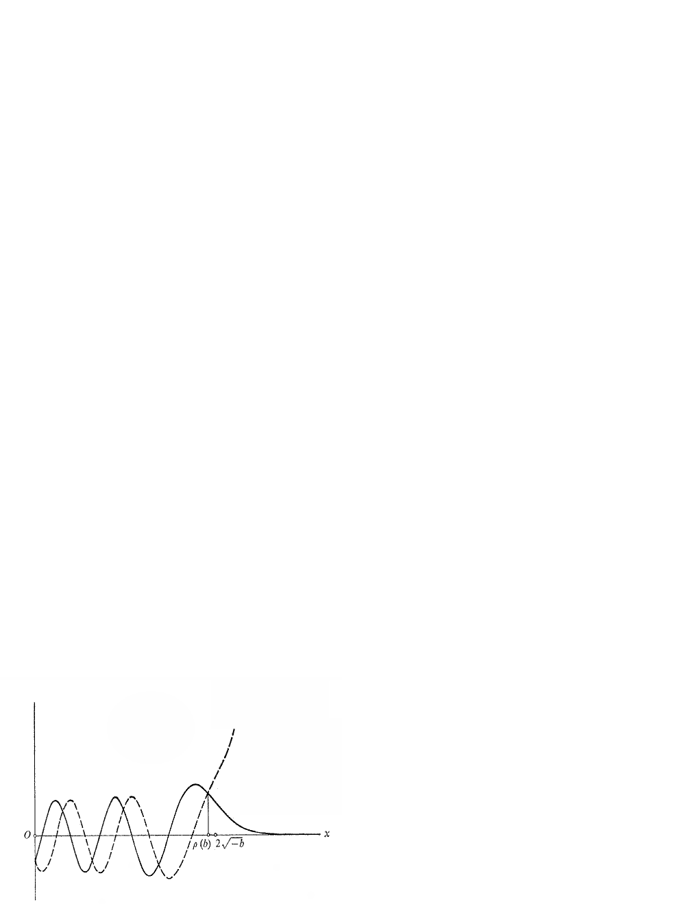
Figure 5. An example of Parabolic Cylinder Functions $U(\cdot;b)$ (continuous) and $\overline{U}(\cdot;b)$ (dashed) for some $b<0$.

To express the errors for the approximations of our problem, we need to define some auxiliary functions having to do with the nature of $U(\cdot,b)$ and $\overline{U}(\cdot,b)$ for negative $b$. In this case the character of each is partly oscillatory and partly exponential, so we introduce one weight function $\mathsf{E}$, two modulus functions $\mathsf{M}$ and $\mathsf{N}$, and finally two phase functions $\theta$ and $\omega$.

We denote by $\rho(b)$ the largest real root of the equation

$$U(x,b)=\overline{U}(x,b).$$

We know (cf. §13 of [18] and the references therein) that $\rho(0)=0$ and $\rho(b)>0$ for $b<0$. Also, $\rho$ is continuous when $b\in(-\infty,0]$. An asymptotic estimate for large negative $b$ is

$$\rho(b)=2\sqrt{-b}+c_{*}(-b)^{-\frac{1}{6}}+\mathcal{O}\big{(}b^{-\frac{5}{6}}\big{)}\quad\text{as}\quad b\to-\infty$$ (B.7)

where $c_{*}$ ($\approx-0.36605$) is the smallest in absolute value root of the equation $\operatorname{Ai}(x)=\operatorname{Bi}(x)$.

For $b\leq 0$ we define

$$\mathsf{E}(x,b)=\begin{cases}1,\quad 0\leq x\leq\rho(b)\\ \Big{[}\frac{\overline{U}(x,b)}{U(x,b)}\Big{]}^{1/2},\quad x>\rho(b).\end{cases}$$

It is seen that $\mathsf{E}$ is continuous in the region $[0,+\infty)\times(-\infty,0]$ of the $(x,b)$-plane and for $b\leq 0$ fixed, $\mathsf{E}(\cdot,b)$ is non-decreasing in the interval $[0,+\infty)$. Again for $b\leq 0$ and $x\geq 0$ we set

$$U(x,b)=\frac{1}{\mathsf{E}(x,b)}\mathsf{M}(x,b)\sin\theta(x,b),\quad\overline{U}(x,b)=\mathsf{E}(x,b)\mathsf{M}(x,b)\cos\theta(x,b)$$

and

$$U^{\prime}(x,b)=\frac{1}{\mathsf{E}(x,b)}\mathsf{N}(x,b)\sin\omega(x,b),\quad\overline{U}^{\prime}(x,b)=\mathsf{E}(x,b)\mathsf{N}(x,b)\cos\omega(x,b).$$

Thus

$$\mathsf{M}(x,b)=\begin{cases}\big{[}U(x,b)^{2}+\overline{U}(x,b)^{2}\big{]}^{1/2},\quad 0\leq x\leq\rho(b)\\ \big{[}2U(x,b)\overline{U}(x,b)\big{]}^{1/2},\quad x>\rho(b)\end{cases}$$ (B.8)

and

$$\theta(x,b)=\begin{cases}\arctan\Big{[}\frac{U(x,b)}{\overline{U}(x,b)}\Big{]},\quad 0\leq x\leq\rho(b)\\ \frac{\pi}{4},\quad x>\rho(b)\end{cases}$$

where the branch of the inverse tangent is continuous and equal to $\frac{\pi}{4}$ at $x=\rho(b)$.

Similarly

$$\mathsf{N}(x,b)=\begin{cases}\Big{[}U^{\prime}(x,b)^{2}+\overline{U}^{\prime}(x,b)^{2}\Big{]}^{1/2},\quad 0\leq x\leq\rho(b)\\ \\ \bigg{[}\frac{U^{\prime}(x,b)^{2}\overline{U}(x,b)^{2}+\overline{U}^{\prime}(x,b)^{2}U(x,b)^{2}}{U(x,b)\overline{U}(x,b)}\bigg{]}^{1/2},\quad x>\rho(b)\end{cases}$$

and

$$\omega(x,b)=\begin{cases}\arctan\Big{[}\frac{U^{\prime}(x,b)}{\overline{U}^{\prime}(x,b)}\Big{]},\quad 0\leq x\leq\rho(b)\\ \\ \arctan\Big{[}\frac{U^{\prime}(x,b)\overline{U}(x,b)}{\overline{U}^{\prime}(x,b)U(x,b)}\Big{]},\quad\quad x>\rho(b)\end{cases}$$

where the branches of the inverse tangents are chosen to be continuous and fixed by $\omega(x,b)\rightarrow-\frac{\pi}{4}$ as $x\rightarrow+\infty$.

For large $x$ we have

$$\mathsf{E}(x,b)\sim\Big{(}\frac{2}{\pi}\Big{)}^{\frac{1}{4}}\Gamma(\tfrac{1}{2}-b)^{\frac{1}{2}}x^{b}e^{\frac{1}{4}x^{2}}$$

and

$$\mathsf{M}(x,b)\sim\Big{(}\frac{8}{\pi}\Big{)}^{\frac{1}{4}}\frac{\Gamma(\tfrac{1}{2}-b)^{\frac{1}{2}}}{x^{\frac{1}{2}}},\quad\mathsf{N}(x,b)\sim\frac{\Gamma(\tfrac{1}{2}-b)^{\frac{1}{2}}}{(2\pi)^{\frac{1}{4}}}x^{\frac{1}{2}}.$$ (B.9)

Both of these hold for fixed $b$ and are also uniform for $b$ ranging over any compact interval in $(-\infty,0]$.

Appendix C A Theorem on Integral Equations

The proofs of theorems about WKB approximation when there is an absence of turning points (like Theorems 2.1 and 2.2 in chapter 6 of [17]), may be adapted to other types of approximate solutions of linear differential equations where turning points may be present. For second-order equations the basic steps consist of

• construction of a Volterra integral equation for the error term -say $h$- of the solution, by the method of variation of parameters

• construction of the Liouville-Neumann expansion (a uniformly convergent series) for the solution $h$ of the integral equation in (i) by Picard’s method of successive approximations

• confirmation that $h$ is twice differentiable by construction of similar series for $h^{\prime}$ and $h^{\prime\prime}$

• production of bounds for $h$ and $h^{\prime}$ by majoring the Liouville-Neumann expansion.

It would be tedious to carry out all these steps in every case. But we have the following general theorem which automatically provides (ii), (iii) and (iv) in problems relevant to us.

Theorem C.1.

Consider the equation

$$h(\zeta)=\int_{\beta}^{\zeta}\mathsf{K}(\zeta,t)\phi(t)\{J(t)+h(t)\}dt$$ (C.1)

for the function $h$ accompanied by the following assumptions

• the path of integration consists of a segment $[\beta,\zeta]$ of the real axis, finite or infinite where $\beta\leq t\leq\zeta\leq\gamma$

• the real functions $J$ and $\phi$ are continuous in $(\beta,\gamma)$ except for a finite number of discontinuities and infinities

• the real kernel $\mathsf{K}$ and its first two partial derivatives with respect to $\zeta$ are continuous functions of both variables when $\zeta,t\in(\beta,\gamma)$

• $\mathsf{K}(\zeta,\zeta)=0,\quad\zeta\in(\beta,\gamma)$

• when $\zeta\in(\beta,\gamma)$ and $t\in(\beta,\zeta]$ we have

  $$|\mathsf{K}(\zeta,t)|\leq P_{0}(\zeta)Q(t),\qquad\Big{|}\frac{\partial\mathsf{K}(\zeta,t)}{\partial\zeta}\Big{|}\leq P_{1}(\zeta)Q(t),\qquad\Big{|}\frac{\partial^{2}\mathsf{K}(\zeta,t)}{\partial\zeta^{2}}\Big{|}\leq P_{2}(\zeta)Q(t)$$

  where the $P_{j},j=0,1,2$ and $Q$ are continuous real functions, the $P_{j},j=0,1,2$ being positive.

• when $\zeta\in(\beta,\gamma)$, the integral

  $$\Phi(\zeta)=\int_{\beta}^{\zeta}|\phi(t)|dt$$

  converges and the following suprema

  $$\kappa=\sup_{\zeta\in(\beta,\gamma)}\{Q(\zeta)|J(\zeta)|\},\qquad\kappa_{0}=\sup_{\zeta\in(\beta,\gamma)}\{P_{0}(\zeta)Q(\zeta)\}$$

  are finite.

Under these assumptions, equation (C.1) has a unique solution $h$ which is continuously differentiable in $(\beta,\gamma)$ and satisfies

$$\frac{h(\zeta)}{P_{0}(\zeta)}\to 0\qquad\frac{h^{\prime}(\zeta)}{P_{1}(\zeta)}\to 0\qquad\text{as}\quad\zeta\downarrow\beta.$$

Furthermore,

$$\frac{|h(\zeta)|}{P_{0}(\zeta)},\frac{|h^{\prime}(\zeta)|}{P_{1}(\zeta)}\leq\frac{\kappa}{\kappa_{0}}[\exp\{\kappa_{0}\Phi(\zeta)\}-1]$$

and $h^{\prime\prime}$ is continuous except at the discontinuities -if any- of $\phi,J$.

Proof.

The proof is a slight variation of that for Theorem 10.1 of chapter 6 in [17]. ∎

We are going to use this theorem to prove the existence and behavior of approximate solutions of the equation

$$\frac{d^{2}\mathcal{Y}}{d\zeta^{2}}=\big{[}\hbar^{-2}(\zeta^{2}-\alpha^{2})+\psi(\zeta,\hbar,\alpha)\big{]}\mathcal{Y}.$$ (C.2)

We have the following

Theorem C.2.

For each value of $\hbar$, assume that the function $\psi(\zeta,\hbar,\alpha)$ is continuous in the region $[0,Z)\times[0,\delta]$ of the $(\zeta,\alpha)$-plane , take $\Omega$ as in (6.3) and consider that

$$\mathcal{V}_{0,Z}[H](\alpha,\hbar)=\int_{0}^{Z}\frac{|\psi(t,\alpha)|}{\Omega(t\sqrt{2\hbar^{-1}})}dt$$

converges uniformly with respect to $\alpha$. Then in this region, equation (C.2) has solutions $\mathcal{Y}_{1}$ and $\mathcal{Y}_{2}$ which are continuous, have continuous first and second partial $\zeta$-derivatives and are given by

$$\mathcal{Y}_{1}(\zeta,\alpha,\hbar)=U(\zeta\sqrt{2\hbar^{-1}},-\tfrac{1}{2}\hbar^{-1}\alpha^{2})+\epsilon_{1}(\zeta,\alpha,\hbar)$$

$$\mathcal{Y}_{2}(\zeta,\alpha,\hbar)=\overline{U}(\zeta\sqrt{2\hbar^{-1}},-\tfrac{1}{2}\hbar^{-1}\alpha^{2})+\epsilon_{2}(\zeta,\alpha,\hbar)$$

where

$$\frac{|\epsilon_{1}(\zeta,\alpha,\hbar)|}{\mathsf{M}(\zeta\sqrt{2\hbar^{-1}},-\tfrac{1}{2}\hbar^{-1}\alpha^{2})},\frac{\Big{|}\frac{\partial\epsilon_{1}}{\partial\zeta}(\zeta,\alpha,\hbar)\Big{|}}{\sqrt{2\hbar^{-1}}\mathsf{N}(\zeta\sqrt{2\hbar^{-1}},-\tfrac{1}{2}\hbar^{-1}\alpha^{2})}\\ \leq\frac{1}{\mathsf{E}(\zeta\sqrt{2\hbar^{-1}},-\tfrac{1}{2}\hbar^{-1}\alpha^{2})}\Big{(}\exp\big{\{}\tfrac{1}{2}(\pi\hbar)^{\frac{1}{2}}l(-\tfrac{1}{2}\hbar^{-1}\alpha^{2})\mathcal{V}_{\zeta,Z}[H](\alpha,\hbar)\big{\}}-1\Big{)}$$ (C.3)

and

$$\frac{|\epsilon_{2}(\zeta,\alpha,\hbar)|}{\mathsf{M}(\zeta\sqrt{2\hbar^{-1}},-\tfrac{1}{2}\hbar^{-1}\alpha^{2})},\frac{\Big{|}\frac{\partial\epsilon_{2}}{\partial\zeta}(\zeta,\alpha,\hbar)\Big{|}}{\sqrt{2\hbar^{-1}}\mathsf{N}(\zeta\sqrt{2\hbar^{-1}},-\tfrac{1}{2}\hbar^{-1}\alpha^{2})}\\ \leq\mathsf{E}(\zeta\sqrt{2\hbar^{-1}},-\tfrac{1}{2}\hbar^{-1}\alpha^{2})\Big{(}\exp\big{\{}\tfrac{1}{2}(\pi\hbar)^{\frac{1}{2}}l(-\tfrac{1}{2}\hbar^{-1}\alpha^{2})\mathcal{V}_{0,\zeta}[H](\alpha,\hbar)\big{\}}-1\Big{)}.$$ (C.4)

Proof.

We will prove the theorem only for the first solution since the proof for the second follows mutatis mutandis. Observe that the approximating function $U(\zeta\sqrt{2\hbar^{-1}},-\tfrac{1}{2}\hbar^{-1}\alpha^{2})$ satisfies $\frac{d^{2}U}{d\zeta^{2}}=\hbar^{-2}(\zeta^{2}-\alpha^{2})U$. If we subtract this from (C.2) we obtain the following differential equation for the error term

$$\frac{d^{2}\epsilon_{1}}{d\zeta^{2}}-\hbar^{-2}(\zeta^{2}-\alpha^{2})\epsilon_{1}=\psi(\zeta,\alpha,\hbar)\big{[}\epsilon_{1}+U(\zeta\sqrt{2\hbar^{-1}},-\tfrac{1}{2}\hbar^{-1}\alpha^{2})\big{]}.$$

By use of the method of variation of parameters and also (B.3) one arrives at the integral equation

$$\epsilon_{1}(\zeta,\alpha,\hbar)=\frac{1}{2}\frac{(\pi\hbar)^{\frac{1}{2}}}{\Gamma\big{(}\frac{1}{2}+\frac{1}{2}\hbar^{-1}\alpha^{2}\big{)}}\int_{\zeta}^{Z}\mathcal{K}(\zeta,t)\psi(t,\alpha,\hbar)\big{[}\epsilon_{1}(t,\alpha,\hbar)+U(t\sqrt{2\hbar^{-1}},-\tfrac{1}{2}\hbar^{-1}\alpha^{2})\big{]}dt$$

in which

$$\mathcal{K}(\zeta,t)=U(\zeta\sqrt{2\hbar^{-1}},-\tfrac{1}{2}\hbar^{-1}\alpha^{2})\overline{U}(t\sqrt{2\hbar^{-1}},-\tfrac{1}{2}\hbar^{-1}\alpha^{2})\\ -U(t\sqrt{2\hbar^{-1}},-\tfrac{1}{2}\hbar^{-1}\alpha^{2})\overline{U}(\zeta\sqrt{2\hbar^{-1}},-\tfrac{1}{2}\hbar^{-1}\alpha^{2}).$$

Bounds for the kernel $\mathcal{K}$ and its first two partial derivatives (with respect to $\zeta$) are expressible in terms of the auxiliary functions $\mathsf{E},\mathsf{M}$ and $\mathsf{N}$. We have

$$|\mathcal{K}(\zeta,t)| \leq\frac{\mathsf{E}(t\sqrt{2\hbar^{-1}},-\tfrac{1}{2}\hbar^{-1}\alpha^{2})}{\mathsf{E}(\zeta\sqrt{2\hbar^{-1}},-\tfrac{1}{2}\hbar^{-1}\alpha^{2})}\mathsf{M}(\zeta\sqrt{2\hbar^{-1}},-\tfrac{1}{2}\hbar^{-1}\alpha^{2})\mathsf{M}(t\sqrt{2\hbar^{-1}},-\tfrac{1}{2}\hbar^{-1}\alpha^{2})$$

$$\bigg{|}\frac{\partial\mathcal{K}}{\partial\zeta}(\zeta,t)\bigg{|} \leq\sqrt{2\hbar^{-1}}\frac{\mathsf{E}(t\sqrt{2\hbar^{-1}},-\tfrac{1}{2}\hbar^{-1}\alpha^{2})}{\mathsf{E}(\zeta\sqrt{2\hbar^{-1}},-\tfrac{1}{2}\hbar^{-1}\alpha^{2})}\mathsf{N}(\zeta\sqrt{2\hbar^{-1}},-\tfrac{1}{2}\hbar^{-1}\alpha^{2})\mathsf{M}(t\sqrt{2\hbar^{-1}},-\tfrac{1}{2}\hbar^{-1}\alpha^{2})$$

and similarly

$$\frac{\partial^{2}\mathcal{K}}{\partial\zeta^{2}}(\zeta,t)=(2\hbar^{-1})^{\frac{3}{2}}\zeta\mathsf{K}(\zeta,t).$$

All these estimates allow us to solve the equation (C.2) by applying Theorem C.1. Using the notation of that theorem we have

$$\phi(t) =\frac{\psi(\zeta,\alpha,\hbar)}{\Omega(\zeta\sqrt{2\hbar^{-1}})}$$

$$\psi_{1}(t) =0$$

$$J(t) =U(t\sqrt{2\hbar^{-1}},-\tfrac{1}{2}\hbar^{-1}\alpha^{2})$$

$$\mathsf{K}(\zeta,t) =-\frac{1}{2}\frac{(\pi\hbar)^{\frac{1}{2}}}{\Gamma\big{(}\frac{1}{2}+\frac{1}{2}\hbar^{-1}\alpha^{2}\big{)}}\Omega(t\sqrt{2\hbar^{-1}})\mathcal{K}(\zeta,t)$$

$$Q(t) =\frac{1}{2}\frac{(\pi\hbar)^{\frac{1}{2}}}{\Gamma\big{(}\frac{1}{2}+\frac{1}{2}\hbar^{-1}\alpha^{2}\big{)}}\Omega(t\sqrt{2\hbar^{-1}})\mathsf{E}(t\sqrt{2\hbar^{-1}},-\tfrac{1}{2}\hbar^{-1}\alpha^{2})\mathsf{M}(t\sqrt{2\hbar^{-1}},-\tfrac{1}{2}\hbar^{-1}\alpha^{2})$$

$$P_{0}(\zeta) =\frac{\mathsf{M}(\zeta\sqrt{2\hbar^{-1}},-\tfrac{1}{2}\hbar^{-1}\alpha^{2})}{\mathsf{E}(\zeta\sqrt{2\hbar^{-1}},-\tfrac{1}{2}\hbar^{-1}\alpha^{2})}$$

$$P_{1}(\zeta) =\sqrt{2\hbar^{-1}}\frac{\mathsf{N}(\zeta\sqrt{2\hbar^{-1}},-\tfrac{1}{2}\hbar^{-1}\alpha^{2})}{\mathsf{E}(\zeta\sqrt{2\hbar^{-1}},-\tfrac{1}{2}\hbar^{-1}\alpha^{2})}$$

$$\Phi(\zeta) =\mathcal{V}_{0,\zeta}[H](\alpha,\hbar)$$

$$\kappa_{0} \leq\frac{1}{2}(\pi\hbar)^{\frac{1}{2}}l(-\tfrac{1}{2}\hbar^{-1}\alpha^{2})$$

where the role of $\beta$ is played here by $Z$ and $\kappa$ is replaced for simplicity by the upper bound $\kappa_{0}$. Then the bounds (C.3) and (C.4) follow from Theorem C.1.

Finally, observe that all the integrals which occur in the analysis above, converge uniformly when $\alpha\in[0,\delta]$ and $\zeta$ lies in any compact interval of $[0,Z)$; allowing us to state that $\epsilon_{1}$ and its first two partial $\zeta$-derivatives are continuous in $\alpha$ and $\zeta$. Consequently, the same stands for $\mathcal{Y}_{1}$ which signifies the end of the proof. ∎

Data Availability

Data sharing is not applicable to this article as no new data were created or analyzed in this study.

References

• [1] M. Abramowitz and I. A. Stegun, Handbook of Mathematical Functions with Formulas, Graphs, and Mathematical Tables, Vol. 55, US Government Printing Office (1948).
• [2] M. Bertola and A. Tovbis Universality for the Focusing Nonlinear Schrödinger Equation at the Gradient Catastrophe Point: Rational Breathers and Poles of the Tritronquée Solution to Painlevé I, Communications in Pure and Applied Mathematics 66, no.5 (2013), pp. 678–752
• [3] T. B. Benjamin and J. E. Feir, The Disintegration of Wavetrains on Deep Water. Part 1. Theory, Journal of Fluid Mechanics 27, no. 3 (1967), pp. 417–430
• [4] J. Ecalle, Cinq Applications des Fonctions Résurgentes, Publ. Math. d’ Orsay (1984).
• [5] S. Fujiié and S. Kamvissis, Semiclassical WKB Problem for the Non-self-adjoint Dirac Operator with Analytic Potential, Journal of Mathematical Physics 61, no. 1 (2020), p. 011510.
• [6] S. Fujiié, C. Lasser and L. Nédélec, Semiclassical Resonances for a Two-level Schrödinger Operator with a Conical Intersection, Asymptotic Analysis 65, no. 1-2 (2009), pp. 17-58.
• [7] C. Gérard and A. Grigis, Precise Estimates of Tunneling and Eigenvalues near a Potential Barrier, J. Differential Equations 72 (1988), pp.149-177.
• [8] N. Hatzizisis, S. Kamvissis, Semiclassical WKB Problem for the Non-Self-Adjoint Dirac Operator with a Multi-Humped Decaying Potential, arXiv:2106.07253.
• [9] S. Kamvissis, K. D. T. R. McLaughlin and P. D. Miller, Semiclassical Soliton Ensembles for the Focusing Nonlinear Schrödinger Equation, Annals of Mathematics 154 (2003), Princeton University Press, Princeton, NJ.
• [10] S. Kamvissis, E. A. Rakhmanov, Existence and Regularity for an Energy Maximization Problem in Two Dimensions, Journal of Mathematical Physics 46, no. 8 (2005)
• [11] M. Klaus and J. K. Shaw, Purely Imaginary Eigenvalues of Zakharov-Shabat Systems, Physical Review E 65, no. 3 (2002), p. 036607.
• [12] M. Klaus and J. K. Shaw, On the Eigenvalues of Zakharov–Shabat Systems, SIAM Journal on Mathematical Analysis 34, no. 4 (2003), pp. 759-773.
• [13] J. C. P. Miller, On the Choice of Standard Solutions for a Homogeneous Linear Differential Equation of the Second Order, The Quarterly Journal of Mechanics and Applied Mathematics 3, no. 2 (1950), pp. 225-235.
• [14] P. D. Miller, Some Remarks on a WKB Method for the Non-selfadjoint Zakharov-Shabat Eigenvalue Problem with Analytic Potentials and Fast Phase, Physica D, Nonlinear Phenomena 152 (2001), pp. 145-162.
• [15] P. D. Miller, S. Kamvissis, On the Semiclassical Limit of the Focusing Nonlinear Schrödinger Equation, Phys. Lett. A 247 (1998), pp. 75–86.
• [16] F. W. J. Olver, Second-Order Linear Differential Equations with Two Turning Points, Philosophical Transactions of the Royal Society of London, Series A, Mathematical and Physical Sciences 278, no. 1279 (1975), pp. 137-174.
• [17] F. W. J. Olver, Asymptotics and Special Functions, AK Peters/CRC Press (1997).
• [18] F. W. J Olver, D. W. Lozier, R. F. Boisvert and C. W. Clark, eds. NIST Handbook of Mathematical Functions (Hardback and CD-ROM), Cambridge University Press (2010).
• [19] A. Voros, The Return of the Quartic Oscillator, the Complex WKB Method, Annales de l’ IHP Physique Théorique 39, no. 3 (1983), pp. 211-338.
• [20] D. R. Yafaev, The Semiclassical Limit of Eigenfunctions of the Schrödinger Equation and the Bohr-Sommerfeld Quantization Condition, Revisited, St. Petersburg Mathematical Journal 22, no. 6 (2011), pp. 1051-1067.
• [21] D. R. Yafaev, Passage Through a Potential Barrier and Multiple Wells, St. Petersburg Mathematical Journal 29, no. 2 (2018), pp. 399-422.
• [22] V. Zakharov and A. Shabat, Exact Theory of Two-dimensional Self-focusing and One-dimensional Self-modulation of Waves in Nonlinear Media, Soviet physics JETP 34, no. 1 (1972), p. 62.