Connectivity of Triangulation Flip Graphs in the Plane

Abstract

Given a finite point set $P$ in general position in the plane, a full triangulation of $P$ is a maximal straight-line embedded plane graph on $P$. A partial triangulation of $P$ is a full triangulation of some subset $P^{\prime}$ of $P$ containing all extreme points in $P$. A bistellar flip on a partial triangulation either flips an edge (called edge flip), removes a non-extreme point of degree 3, or adds a point in $P\setminus P^{\prime}$ as vertex of degree 3. The bistellar flip graph has all partial triangulations as vertices, and a pair of partial triangulations is adjacent if they can be obtained from one another by a bistellar flip. The edge flip graph is defined with full triangulations as vertices, and edge flips determining the adjacencies. Lawson showed in the early seventies that these graphs are connected. The goal of this paper is to investigate the structure of these graphs, with emphasis on their vertex connectivity.

For sets $P$ of $n$ points in the plane in general position, we show that the edge flip graph is $\lceil\frac{n}{2}-2\rceil$-vertex connected, and the bistellar flip graph is $(n-3)$-vertex connected; both results are tight. The latter bound matches the situation for the subfamily of regular triangulations (i.e., partial triangulations obtained by lifting the points to 3-space and projecting back the lower convex hull), where $(n-3)$-vertex connectivity has been known since the late eighties through the secondary polytope due to Gelfand, Kapranov & Zelevinsky and Balinski’s Theorem. For the edge flip-graph, we additionally show that the vertex connectivity is as least as large as (and hence equal to) the minimum degree (i.e., the minimum number of flippable edges in any full triangulation), provided that $n$ is large enough.

Our methods also yield several other results: (i) The edge flip graph can be covered by graphs of polytopes of dimension $\lceil\frac{n}{2}-2\rceil$ (products of associahedra) and the bistellar flip graph can be covered by graphs of polytopes of dimension $n-3$ (products of secondary polytopes). (ii) A partial triangulation is regular, if it has distance $n-3$ in the Hasse diagram of the partial order of partial subdivisions from the trivial subdivision. (iii) All partial triangulations of a point set are regular iff the partial order of partial subdivisions has height $n-3$. (iv) There are arbitrarily large sets $P$ with non-regular partial triangulations and such that every proper subset has only regular triangulations, i.e., there are no small certificates for the existence of non-regular triangulations.

Keywords.

triangulation, regular triangulation, flip graph, bistellar flip graph, graph connectivity, associahedron, secondary polytope, subdivision, convex decomposition, polyhedral subdivision, flippable edge, simultaneously flippable edges, pseudo-simultaneously flippable edges, flip complex, Menger’s Theorem, Balinski’s Theorem, $k$-hole.

1 Introduction

Triangulations of point sets play a role in many areas including mathematics, numerics, computer science, and processing of geographic data, [14, 11, 4, 24]. A natural way to provide structure to the set of all triangulations is to consider a graph, called flip graph, with the triangulations as vertices and with pairs of triangulations adjacent if they can be obtained from each other by a minimal local change, called a flip (see below for the precise definition). One of the first and most prominent results on flip graphs of planar points sets (for edge flips), proved by Lawson [23] in 1972, is that they are connected. The corresponding question of connectedness of flip graphs in higher dimensions remained a mystery until Santos [32] showed, in 2000, that in dimension $5$ and higher, there exist point sets for which the graph (for bistellar flips) is not connected. The question is still open in dimension $3$ and $4$.

Here, we concentrate on point sets in general position in the plane and investigate “how” connected the flip graphs are, i.e., determine the largest $k$ (in terms of $n$, the size of the underlying point set) such that $k$-vertex connectivity holds. Moreover, we supply some structural results for the flip graph.

The preceding discussion swept under the rug that there are several types of triangulations, most prominently full triangulations (as mostly considered in computational geometry), partial triangulations (as primarily considered in discrete geometry), and regular triangulations (also called coherent triangulations or weighted Delaunay triangulations). We will address the vertex-connectivity for full and partial triangulations, and we will discuss some implications for regular triangulations, for which the vertex-connectivity of the flip graph has been known since the late eighties via the secondary polytope introduced by Gelfand et al. [17] (see [11, Cor. 5.3.2]).

Let us first supply the basic definitions and then discuss the results in more detail.

Definition 1.1 (point set).

Throughout this paper we let $P$ denote a finite planar point set in general position (i.e., no three points on a line) with $n\geq 3$ points. The set of extreme points of $P$ (i.e., the vertices of the convex hull of $P$) is denoted by ${\sf xtr}P$, and we let $P^{\circ}:=P\setminus{\sf xtr}P$ denote the set of inner (i.e., non-extreme) points in $P$. We consistently use the notation $h=h(P):=|{\sf xtr}P|$ and $n^{\!\circ}=n^{\!\circ}(P):=|P^{\circ}|=n-h$, and we let ${\sf E_{\mathsf{hull}}}={\sf E_{\mathsf{hull}}}(P)\subseteq{P\choose 2}$ denote the set of edges of the convex hull of $P$, $|{\sf E_{\mathsf{hull}}}|=h$.

Definition 1.2 (plane graph).

For graphs $G=(P^{\prime},E)$, $P^{\prime}\subseteq P$, $E\subseteq{P^{\prime}\choose 2}$, on $P^{\prime}$ we often identify edges $\{p,q\}\in E$ with their corresponding straight line segments $pq$. We let $\mathrm{\sf V}G:=P^{\prime}$ and $\mathrm{\sf E}G:=E$.

A graph $G$ on $P$ is plane if no two straight line segments corresponding to edges in $\mathrm{\sf E}G$ cross (i.e., they are disjoint except for possibly sharing an endpoint). For $G$ plane, the bounded connected components of the complement of the union of the edges are called regions, the set of regions of $G$ is denoted by $\mathrm{\sf R}G$.

Note that regions are open sets. Note also that isolated points in a plane graph are ignored in the definition of regions.

Definition 1.3 (full, partial, regular triangulation).

1. A full triangulation of $P$ is a maximal plane graph $T=(P,E)$.

2. A partial triangulation of $P$ is a full triangulation $T=(P^{\prime},E)$ with ${\sf xtr}P\subseteq P^{\prime}\subseteq P$ (hence ${\sf E_{\mathsf{hull}}}\subseteq\mathrm{\sf E}T$).

3. A regular triangulation of $P$ is a triangulation obtained by projecting (back to $\mathbb{R}^{2}$) the edges of the lower convex hull of a generic lifting of $P$ to $\mathbb{R}^{3}$ (i.e., we add third coordinates to the points in $P$ so that no four lifted points are coplanar).

Points in $\mathrm{\sf V^{\circ}}T:=P^{\circ}\cap\mathrm{\sf V}T$ are called inner points of $T$ and points in $P^{\circ}\setminus\mathrm{\sf V^{\circ}}T$ are called skipped in $T$ (clearly, for a full triangulation $\mathrm{\sf V^{\circ}}T=P^{\circ}$ and no points are skipped). Edges in $\mathrm{\sf E^{\circ}}T:=\mathrm{\sf E}T\setminus{\sf E_{\mathsf{hull}}}$ are called inner edges and edges in ${\sf E_{\mathsf{hull}}}$ are called boundary edges.

${\cal T}_{\mathsf{full}}(P)$, ${\cal T}_{\mathsf{part}}(P)$, and ${\cal T}_{\mathsf{reg}}(P)$ will denote the set of all full, partial, and regular triangulations of $P$, respectively.

Every full and every regular triangulation of $P$ is also a partial triangulation of $P$. If $P$ is in convex position (i.e., ${\sf xtr}P=P$), all three notions coincide. It is well-known, that there are point sets with non-regular triangulations, [11], see Sec. 10.2 and Fig. 29.

Definition 1.4 (edge flip, point insertion flip, point removal flip).

Let $T\in{\cal T}_{\mathsf{part}}(P)$.

An edge $e\in\mathrm{\sf E^{\circ}}T$ is called flippable in $T$ if removing $e$ from $T$ creates a convex quadrilateral region $Q$. In this case, we denote by $T[e]$ the triangulation with the other diagonal $\overline{e}$ of $Q$ added instead of $e$, i.e., $\mathrm{\sf V}T[e]:=\mathrm{\sf V}T$ and $\mathrm{\sf E}T[e]:=\mathrm{\sf E}T\setminus\{e\}\cup\{\overline{e}\}=\mathrm{\sf E}T\oplus\{e,\overline{e}\}$; we call this an edge flip. Occasionally, when we want to emphasize the new edge $\overline{e}$, we will also use the alternative notation $T[\nicefrac{{e}}{{\overline{e}}}]$ instead of $T[e]$, or write $T[e]=T[\nicefrac{{e}}{{\overline{e}}}]$.

A point $p\in P^{\circ}$ is called flippable in $T$ if $p\in P^{\circ}\setminus\mathrm{\sf V^{\circ}}T$, or if $p\in\mathrm{\sf V^{\circ}}T$ is of degree $3$ in $T$. (a) If $p\in P^{\circ}\setminus\mathrm{\sf V^{\circ}}T$ then $T[p]$ is the triangulation with $p$ added as a point of degree $3$ (there is a unique way to do so); we call this a point insertion flip. (b) If $p\in\mathrm{\sf V^{\circ}}T$ is of degree $3$ in $T$ then $T[p]$ is obtained by removing $p$ and its incident edges; we call this a point removal flip. See Fig. 1.

A bistellar flip is one of the three: an edge flip, a point insertion flip, or a point removal flip.

                          

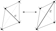
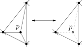
Figure 1: Edge flips and point flips (point removal, left to right; point insertion, right to left).

Hence, whenever we write $T[x]$ for a partial triangulation $T$, then $x$ is either a flippable point in $P^{\circ}$ or a flippable edge in $\mathrm{\sf E^{\circ}}T$. We will use $T[x,y]$ short for $(T[x])[y]$, etc.

Definition 1.5 (bistellar flip graph, edge flip graph).

The bistellar flip graph of $P$ is the graph with vertex set ${\cal T}_{\mathsf{part}}(P)$ and edge set $\{\{T,T[x]\}\,|\,T\in{\cal T}_{\mathsf{part}}(P)\mbox{, $x\in P^{\circ}\cup\mathrm{\sf E^{\circ}}T$ flippable in~{}}T\}$.

The edge flip graph of $P$ is the graph with vertex set ${\cal T}_{\mathsf{full}}(P)$ and edge set $\{\{T,T[e]\}\,|\,T\in{\cal T}_{\mathsf{full}}(P)\mbox{, $e\in\mathrm{\sf E^{\circ}}T$ flippable in~{}}T\}$. See Figures 2 and 3 for examples.

       

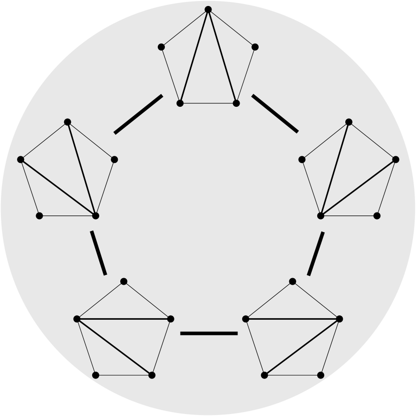
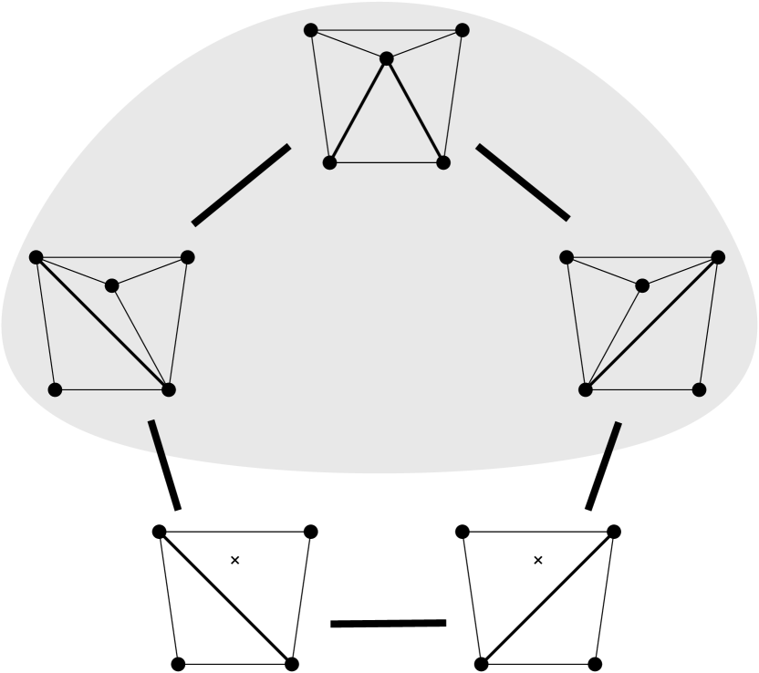
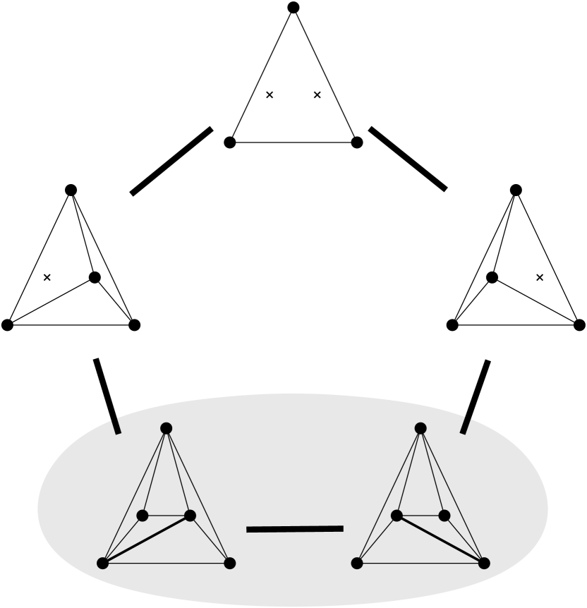
Figure 2: Bistellar flip graphs for $5$ points. Small crosses indicate skipped points in $P$. The shaded areas contain the edge flip graph, the subgraph induced by full triangulations.

 

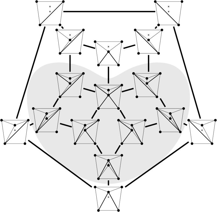
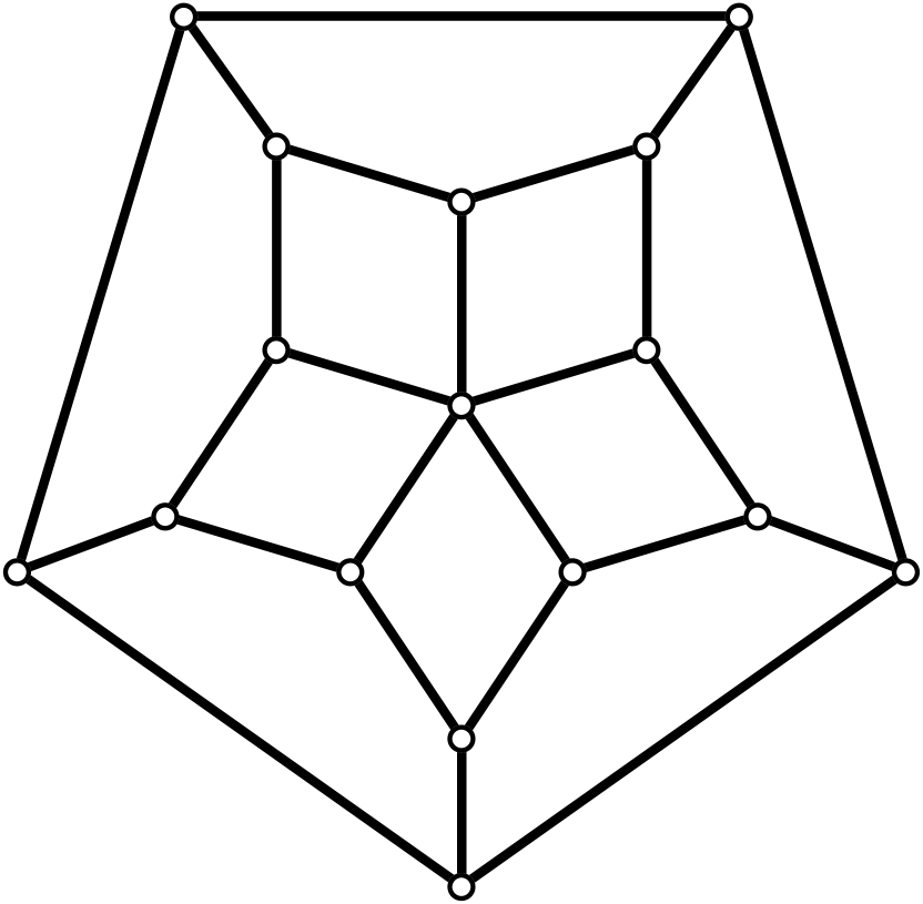
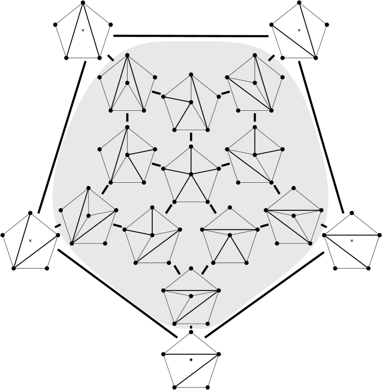
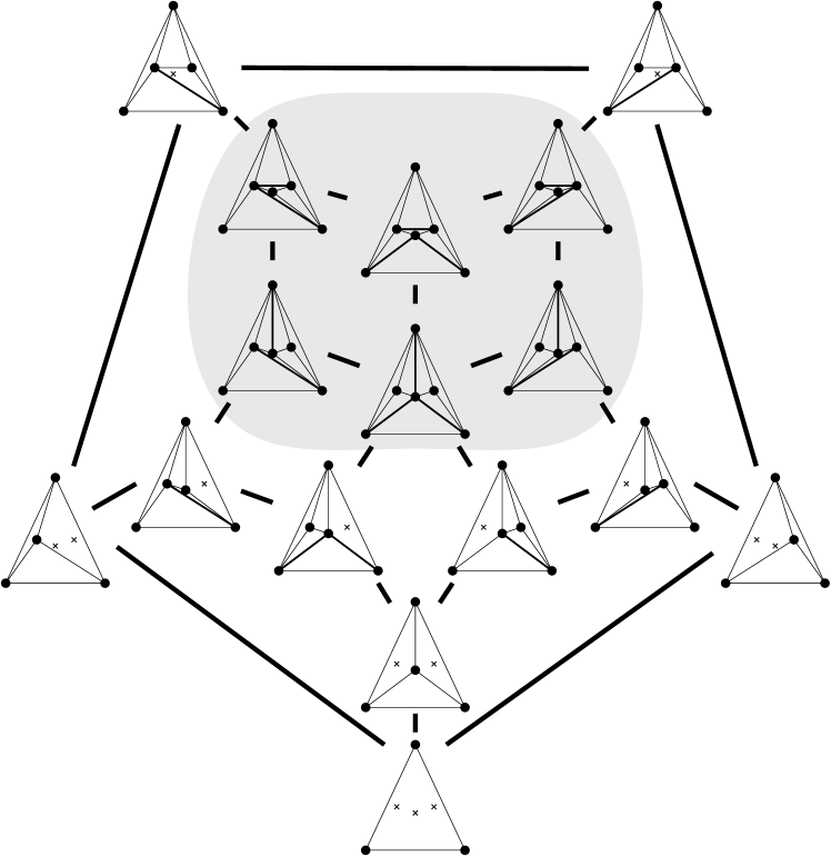
Figure 3: Sets of $6$ points with isomorphic bistellar flip graphs of partial triangulations. The shaded areas cover the edge flip graphs of full triangulations. (Crosses indicate skipped points.)

1.1 Results – full triangulations

The edge flip graph is the subgraph of the bistellar flip graph induced by ${\cal T}_{\mathsf{full}}(P)$ (see Figures 2 and 3). Lawson [23] showed that the edge flip graph is connected. A trivial upper bound for the vertex connectivity (see Def. 2.1) of any graph is the minimum vertex degree of the graph; for the edge flip graph this is the minimum number of flippable edges in any triangulation of $P$. This number has been investigated by Hurtado et al. in 1999, [22, Thm. 4.1].

Theorem 1.6 ([22]).

Any $T\in{\cal T}_{\mathsf{full}}(P)$ has at least $\lceil\frac{n}{2}-2\rceil$ flippable edges. This bound is tight for all $3\leq n\in\mathbb{N}$  (i.e., for every $n$ there is a set $P$, $|P|=n$, with a triangulation with exactly $\lceil\frac{n}{2}-2\rceil$ flippable edges).

We provide a lower bound on the vertex connectivity of the edge flip graph that matches this lower bound of $\lceil\frac{n}{2}-2\rceil$ for the minimum vertex degree, actually in the refined form $\max\{\lceil\frac{n}{2}-2\rceil,h-3\}$, see Hoffmann et al. [20]. Note, however, that there are sets of points where all full triangulations allow more than $\max\{\lceil\frac{n}{2}-2\rceil,h-3\}$ edge flips. We show that, for $P$ large enough, the minimum vertex degree always determines the vertex connectivity of the edge flip graph.

Theorem 1.7.

1. There exists $n_{0}\in\mathbb{N}$, such that the edge flip graph of any set of $n\geq n_{0}$ points in general position in the plane is $\delta$-vertex connected, where $\delta$ is the minimum vertex degree in the edge flip graph.

2. For $5\leq n\in\mathbb{N}$, the edge flip graph of any set of $n$ points with $h$ extreme points in general position is $\max\{\lceil\frac{n}{2}-2\rceil,h-3\}$-vertex connected. This is tight: For every $n\in\mathbb{N}$ there is a triangulation of some set of $n$ points with no more than $\max\{\lceil\frac{n}{2}-2\rceil,h-3\}$ flippable edges.

Obviously, for $n\geq n_{0}$, (i) implies (ii). In fact, we do not know whether the restriction “$n$ large enough” is required in (i). Still, apart from covering the range to $n_{0}$, we consider the proof for (ii) of independent interest, since it provides some extra insight to the structure of the edge flip graph via so-called subdivisions, and it is an introduction to the proof for the bistellar flip graph.

1.2 Results – partial triangulations

The bistellar flip graph is connected, as it follows easily from the connectedness of the edge flip graph, see [11, Sec. 3.4.1]. Here is the counterpart of Thm. 1.6 addressing the minimum vertex degree in the bistellar flip graph, shown by De Loera et al. in 1999, [12, Thm. 2.1].

Theorem 1.8 ([12]).

Any $T\in{\cal T}_{\mathsf{part}}(P)$ allows at least $n-3$ flips. This bound is tight for all $P$.

Again, we show that the vertex connectivity equals the minimum degree.

Theorem 1.9.

Let $4\leq n\in\mathbb{N}$. The bistellar flip graph of any set of $n$ points in general position in the plane is $(n-3)$-vertex connected. This is tight: Any triangulation of a point set that skips all inner points has degree $n-3$ in the bistellar flip graph.

This answers (for points in general position) a question mentioned by De Loera, Rambau & Santos in 2010, [11, Exercise 3.23], and by Lee & Santos in 2017, [24, pg. 442].

Before we mention further results, we provide some context. Along the way, we encounter some tools and provide intuition relevant later in the paper.

1.3 Context – convex position, associahedron, and Balinski’s Theorem

Suppose $P$ is in convex position. Then ${\cal T}_{\mathsf{full}}(P)={\cal T}_{\mathsf{part}}(P)={\cal T}_{\mathsf{reg}}(P)$ is the set of triangulations of a convex $n$-gon whose study goes back to Euler, with one of the first appearances of the Catalan Numbers. There is an $(n-3)$-dimensional convex polytope, the associahedron, whose vertices correspond to the triangulations of a convex $n$-gon, and whose edges correspond to edge flips between these triangulations, see [9] for a historical account. That is, the 1-skeleton (graph) of this polytope is isomorphic to the flip graph of $P$, see Fig. 2(left) for $n=5$ and Fig. 4 for $n=6$. Here Balinski’s Theorem from 1961 comes into play.

         

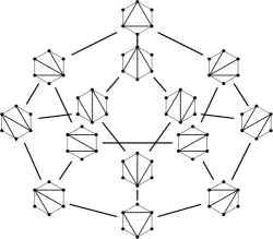
Figure 4: The flip graph of a convex hexagon, the graph of the 3-dimensional associahedron.

Theorem 1.10 (Balinski’s Theorem, [3]).

The 1-skeleton of a convex $d$-dimensional polytope is at least $d$-vertex connected.

Thus we can conclude that the flip graph of $n$ points in convex position is $(n-3)$-vertex connected. The face structure of the associahedron is easily explained via so-called subdivisions (also known as polyhedral subdivisions or convex decompositions), which will feature prominently in our arguments. Specialized to the setting of convex position, a subdivision $S$ is a plane graph on $P$ with all boundary edges present, and some diagonals. We identify every such subdivision with the set of all its possible completions to a triangulation (which we will call refinements). Fig. 5 illustrates on two examples for $n=6$, that if $S$ misses $i$ edges towards a triangulation, then its completions to triangulations correspond to the vertices of an $i$-face of the associahedron; in particular, no edge missing (a triangulation) corresponds to a vertex, and one edge missing corresponds to an edge (a flip). This correspondence will guide our intuition, even in more general settings in which there is no polytope in the background.

         

Figure 5: A subdivision $S_{1}$ with one edge missing representing an edge (1-face) of the 3-dimensional associahedron, and a subdivisions $S_{2}$ with two edges missing representing a facet (2-face).

1.4 Context – regular triangulations and secondary polytope

All examples of bistellar flip graphs we have seen so far – Figures 2 and 3, and sets in convex position – are graphs of polytopes, which is not true in general. The reason is simply that for the underlying point sets in these examples all partial triangulations are regular. Specifically, there is the following generalization of the associahedron, a highlight of the topic of triangulations from the late eighties due to Gelfand et al. [17] (see [11, Thm. 5.1.9]) (here specialized to points in the plane).

Theorem 1.11 (secondary polytope, [17]).

For every set $P$ of $n$ points in general position in the plane, there is an $(n-3)$-dimensional polytope $\Sigma\mbox{-}\mathsf{poly}(P)$, the secondary polytope of $P$, whose 1-skeleton is isomorphic to the bistellar flip graph of regular triangulations of $P$.

Again, with the help of Balinski’s Theorem (Thm. 1.10), we immediately get: The bistellar flip graph of regular triangulations of $P$ is $(n-3)$-vertex connected. Our Thm. 1.9 is the corresponding result for the bistellar flip graph of all partial triangulations. Note, however, that it is not a generalization, since it does not imply the result for regular triangulations.

1.5 Context – simplicial complex of plane graphs and its dual flip complex

A polytopal representation of the edge flip graph or the bistellar flip graph of all partial triangulations is not known. In fact, a clean result as with the secondary polytope is not possible (see [11] for details). However, there is a construction, due to Orden & Santos [30], of a simple high-dimensional polytope whose $1$-skeleton represents all so-called pseudo-triangulations of a planar point set and flips between them, following an earlier construction by Rote et al. [31] of a corresponding polytope for pointed pseudo-triangulations.

Moreover, the edge flip graph of full triangulations of a planar point set does form the $1$-skeleton of a closely related higher-dimensional structure, the flip complex, first described by Orden & Santos [30] and later rediscovered by Lubiw et al. [25]. The flip complex is not a polytope, but it is a polytopal complex (informally, a collection of convex polytopes that intersect only in common faces) with a particularly simple topology (it is homotopy equivalent to a ball). For the reader familiar with these notions, we briefly review how our findings fit into this context (for a quick reference for the relevant terminology from topology theory, see, e.g., [5]). This is not essential as a tool for our proofs and the rest of the paper can be followed without this context. Rather, our results shed some extra light on these structures considered in the literature.

Following [25], let us consider

$$\mathbb{T}:=\mathbb{T}(P)=\{\mbox{$E\subseteq{P\choose 2}$}\mid\mbox{~{}no two edges in $E$ cross}\},$$

i.e., these are the edge sets of plane graphs on $P$. Since this family of sets is closed under taking subsets, it is a simplicial complex, and we call its elements faces of $\mathbb{T}$. By definition, the dimension of a face $F\in\mathbb{T}$ is $\dim F:=|F|-1$. The inclusion-maximal faces (called facets of $\mathbb{T}$) are exactly the edge sets of full triangulations of $P$. All facets have equal dimension $m-1$ (where $m:=3n-h-3$, see Lemma 4.6).

In [25], it is shown that $\mathbb{T}$ is shellable and homeomorphic to an $(m-1)$-dimensional ball (this also follows also from the results in [30]). This fact was instrumental in the proof of the so-called orbit conjecture regarding flips in edge-labeled full triangulations formulated in [7] and proved in [25].

A face $F$ of dimension $m-2$ is a plane graph on $P$ with exactly one edge missing towards a full triangulation. If $F$ is obtained from a full triangulation by removal of a flippable edge, there are exactly two ways to complete it to a triangulation – we call $F$ an interior $(m-2)$-face; otherwise, there is exactly one way to do so – we call $F$ a boundary $(m-2)$-face. A face of any dimension is called a boundary face if it is contained in a boundary $(m-2)$-face, and it is called an interior face, otherwise (hence, all facets are interior faces). We have the following, [25, Prop. 3.7].

Theorem 1.12 ([25]).

$F\in\mathbb{T}$ is an interior face iff ${\sf E_{\mathsf{hull}}}\subseteq F$, and all bounded regions of $F$ are convex; (in other words, iff $(P,F)$ is what we will call a subdivision, see Def. 4.1 and also discussion in Sec. 1.3).

From the Coarsening Lemma 4.10 in Sec. 4, the following property of $\mathbb{T}$ is implied.

Theorem 1.13.

Every interior face $F$ of $\mathbb{T}$ contains an interior face of dimension $m+1-\lceil\frac{n}{2}\rceil$.

The flip graph can be seen as a structure dual to $\mathbb{T}$, with the vertices of the flip graph corresponding to the facets of $\mathbb{T}$, and two vertices adjacent in the flip graph, if the corresponding facets of $\mathbb{T}$ share (i.e., contain) a common $(m-2)$-face (which is clearly interior). This can be generalized to the flip complex $\mathbb{X}=\mathbb{T}^{*}$, see [25], with each face of $\mathbb{X}$ (which is dual to an interior face of $\mathbb{T}$) corresponding to a subdivision as we define it below (see Thm. 1.12 above). Each such face is a product of associahedra, and the vertices of such a face of the flip complex are the triangulations refining this subdivision (Def. 4.2). In terms of the flip complex, the Coarsening Lemma 4.10 and Thm. 1.13 can be restated as saying that every inclusion-maximal face of the flip complex is of dimension at least $\max\{\frac{n}{2}-2,h-3\}$ (see also Thm. 6.1).

1.6 Results – regular triangulations

We study the (well-known, see [11]) partially ordered sets of full and partial subdivisions of $P$, respectively (see Definitions 4.1 and 7.1), in which triangulations are the minimal elements. We introduce the notions of slack of a subdivision (Definitions 4.5 and 7.2), perfect coarsening (Def. 8.1) and perfect coarsener (Def. 8.2), and we prove the so-called Coarsening Lemmas 4.10 and 8.6 (these can be considered extensions of Theorems 1.6 and 1.8). We consider these notions and lemmas our main contributions besides Theorems 1.7 and 1.9. Together with a sufficient condition for the regularity of partial triangulations and subdivisions (Thm. 10.1 and Regularity Preservation Lemma 10.10), these yield several other results on the structure of flip graphs. In particular, they allow us to settle, in the unexpected direction, a question by F. Santos [33] regarding the size of certificates for the existence of non-regular triangulations of a given point set in the plane.

Theorem 1.14.

For all $n\in\mathbb{N}$ there is a set of at least $n$ points in general position in the plane, which has non-regular triangulations, and for which any proper subset has only regular triangulations (in other words, only full triangulations of the set can be non-regular).

This should be seen in contrast with the situation in higher dimensions. In large enough dimension, every point set with non-regular triangulations has a subset of bounded size (in the dimension) with non-regular triangulations. This holds since, (a) the vertices of any realization of the cyclic polytope with 12 vertices in dimension 8 has non-regular triangulations, [10] (see [11, Sec. 5.5.2]), and (b) every large enough set of points in general position in $\mathbb{R}^{8}$ has a subset of 12 points which are vertices of a cyclic polytope (this follows from Ramsey’s Theorem, [18, 15, 36]).

1.7 Approach

All our vertex connectivity bounds rely on a local variant of Menger’s Theorem, the Local Menger Lemma 2.3. This lemma says that, assuming connectedness, in order to show $k$-vertex connectivity, it is enough to show $k$ internally vertex-disjoint paths between any two vertices at distance $2$. Then, in order to establish the min-degree bound of Thm. 1.7(i), we explicitly construct the necessary paths between vertices at distance $2$, i.e., triangulations $T[e]$ and $T[f]$.

For the bounds in Theorems 1.7(ii) and 1.9, we look at the neighborhood of a triangulation $T$ (which is in one-to-one correspondence with the flippable elements in $T$), supplied with a compatibility relation between the flippable elements (for the edge flip graph, two flippable edges $e$ and $f$ are compatible, if $e$ remains flippable after flipping $f$, Def. 3.6). We call this the link of $T$, a structure motivated by the vertex figure of a vertex in a polytope, see [39, pg. 54]: Recall that for a vertex $v$ in a $d$-polytope ${\cal P}$, its vertex figure is the $(d-1)$-polytope ${\cal P}^{\prime}$ obtained by intersecting ${\cal P}$ with a hyperplane that separates $v$ from the remaining vertices of the polytope. Vertices of ${\cal P}^{\prime}$ correspond to edges of ${\cal P}$ incident to $v$, edges in the graph of ${\cal P}^{\prime}$ correspond to $2$-faces of ${\cal P}$ incident to $v$. As indicated in Fig. 6, there is a natural way of mapping paths in the graph of ${\cal P}^{\prime}$ to paths in the graph of ${\cal P}$.

Figure 6: The vertex figure of a polytop, with the mapping of paths in the vertex figure to the 1-skeleton of the polytope indicated.

Using the Local Menger Lemma 2.3, this can be easily made an inductive proof of Balinski’s Theorem (Thm. 1.10). We follow exactly this line of thought for flip graphs (where 4- and 5-cycles will play the role of 2-faces), except that we will not need induction: The link of a triangulation avoids 4-cycles in its complement, which turns out to directly yield sufficient vertex connectivity (Lemma 2.4).

That is, we borrow intuition from polytope theory, although we know that the edge flip graph and the bistellar flip graph are in general not graphs of polytopes. However, as we will see in Sections 6 and 11.1, the edge flip graph and the bistellar flip graph can be covered by graphs of $\lceil\frac{n}{2}-2\rceil$- and $(n-3)$-polytopes, respectively.

It is perhaps worthwhile to mention, that interestingly our proofs never supply insight about the flip graphs to be connected, this is assumed and never proved here. That is, the techniques will probably not be able to say something about the connectedness of flip graphs in higher dimension (3 and 4, where this question is open). If at all, it might help analyzing the vertex connectivity of the connected components of flip graphs.

1.8 Paper organization

In Sec. 2 we show the two lemmas on graph connectivity we mentioned already in Sec. 1.7: The Local Menger Lemma and a lemma about the vertex connectivity of graphs with no 4-cycle in their complement. These may be of independent interest, if only as exercises after teaching Menger’s Theorem in class.

Then the paper splits in three parts, where the second and third part on partial triangulations is largely independent of the first part about full triangulations.

1. Sec. 3 shows the min-degree bound of Thm. 1.7(i). Sec. 4 prepares the proof of Thm. 1.7(ii), which is presented in Sec. 5. We prove the Unoriented Edges Lemma 4.9, which captures the essence of and entails Theorems 1.6 (from [22]) and 1.8 (from [12]) above. It allows us to extend them further for our purposes. Moreover, along the way, we give a short proof of the bound for so-called simultaneously flippable edges by Souvaine et al. [35], and we indicate, how it may help getting in insight on so-called $k$-holes in point sets, [34]. In Sec. 6 we briefly indicate polytopal substructures in the edge flip graph.

2. Sections 7-9 show the $(n-3)$-bound in Thm. 1.9.

3. Building on the tools developed in Sections 7-9, in particular the Coarsening Lemma 8.6, Sec. 10 proves a nontrivial new sufficient condition for the regularity of partial triangulations (Thm. 10.1), which can be considered as a generalization of the regularity of stacked triangulations (i.e., triangulations obtained by successively adding points of degree $3$ to a triangulation of ${\sf xtr}P$). This will give us a number of implications to be presented in Sec. 11: Covering the bistellar flip graph by graphs of $(n-3)$-polytopes, a characterization of point sets for which all partial triangulations are regular, and, finally, Thm. 1.14 on the size of certificates for the existence of non-regular triangulations in ${\cal T}_{\mathsf{part}}(P)$.

We conclude by discussing open problems in Sec. 12.

2 Graph Connectivity

We follow the graph theory books of Bollobás, [6], and Diestel, [13].

Definition 2.1.

For $k\in\mathbb{N}$, a simple undirected graph $G$ is $k$-vertex connected if $G$ is connected, has at least $k+1$ vertices, and removing any set of at most $k-1$ vertices (and their incident edges) leaves the graph connected.

Note that a graph is $1$-vertex connected iff it is connected and has at least two vertices. Here is a classical result due to Menger from 1927, [28], see [6, Theorem III.5].

Theorem 2.2 (Menger’s Theorem, [28]).

Let $u$ and $v$ be distinct nonadjacent vertices of a graph $G$. Then the minimal number of vertices separating $u$ from $v$ is equal to the maximal number of internally vertex-disjoint $u$-$v$ paths.

Convention.

From now on, we we will use vertex-disjoint short for “internally vertex-disjoint.”

We will need a local variant of Menger’s Theorem.

Lemma 2.3 (Local Menger).

Let $k\in\mathbb{N}$ and let $G$ be a simple undirected graph. Assume that $G$ is connected. Then $G$ is $k$-vertex connected iff $G$ has at least $k+1$ vertices and for any pair of vertices $u$ and $v$ at distance $2$ there are $k$ pairwise vertex-disjoint $u$-$v$-paths.

Proof. The direction $(\Rightarrow)$ follows from Menger’s Theorem 2.2. For $(\Leftarrow)$, suppose that for any pair $u$ and $v$ of vertices at distance 2 there are $k$ pairwise vertex-disjoint $u$-$v$-paths. We show that no pair of vertices $x$ and $y$ can be separated by removal of a set $V^{\prime}$ of at most $k-1$ vertices (different from $x$ and $y$). This is true for $x$ and $y$ adjacent. If $x$ and $y$ are not adjacent, let $(x=x_{0},x_{1},\ldots,x_{\ell}=y)$ be an $x$-$y$-path which uses the minimal number of vertices in $V^{\prime}$, and among those, a shortest such path (hence $\{x_{i-1},x_{i+1}\}\notin\mathrm{\sf E}G$ for $0<i<\ell$). If no vertex on this path is in $V^{\prime}$ we are done. Otherwise, consider $x_{i}\in V^{\prime}$, $0<i<\ell$. We can replace the subpath $(x_{i-1},x_{i},x_{i+1})$ by an $x_{i-1}$-$x_{i+1}$-path using none of the vertices in $V^{\prime}$ as internal vertices ($x_{i-1}$ and $x_{i+1}$ have distance $2$ and hence such a path exists, since there are $k$ vertex-disjoint $x_{i-1}$-$x_{i+1}$-paths and $|V^{\prime}|<k$). We obtain an $x$-$y$-walk with one less overlap with $V^{\prime}$, and we can turn this into an $x$-$y$-path with less overlap with $V^{\prime}$; contradiction.

For the proofs of Theorems 1.7(ii) and 1.9, here is a special property of a graph that guarantees that the minimum vertex degree determines exactly the vertex connectivity. As briefly discussed in Sec. 1.7, we will apply this lemma not directly to the flip graph, but rather to the link, a neighborhood structure of a triangulation.

Lemma 2.4.

Let $G$ be a graph with its complement having no cycle of length $4$, i.e., for any sequence $(x_{0},x_{1},x_{2},x_{3})$ of four distinct vertices in $G$ there exists $i\in\{0,1,2,3\}$ with $\{x_{i},x_{i+1\!\bmod\!4}\}\in\mathrm{\sf E}G$. Then $G$ is $\delta$-vertex connected, where $\delta$ is the minimum vertex-degree in $G$.

Proof. It suffices to show that for any two distinct nonadjacent vertices $u$ and $v$ there are $\delta$ vertex-disjoint $u$-$v$-paths. Let $z_{1},z_{2},\ldots,z_{\ell}$ be the set of vertices adjacent both to $u$ and to $v$. This gives $u$-$v$-paths $(u,z_{i},v)$, $1\leq i\leq\ell$. If $\ell\geq\delta$ we are done. Otherwise, there are vertices $x_{\ell+1},\ldots,x_{\delta}$ adjacent to $u$ and not to $y$, and there are vertices $y_{\ell+1},\ldots,y_{\delta}$ adjacent to $v$ and not to $u$. For $\ell<j\leq\delta$ consider the sequence $(u,y_{j},x_{j},v)$: None of $\{u,y_{j}\}$, $\{x_{j},v\}$, and $\{u,v\}$ are edges in $G$, hence $\{y_{j},x_{j}\}\in\mathrm{\sf E}G$ and $(u,x_{j},y_{j},v)$ is a $u$-$v$-path. That is, we have found another $\delta-\ell$ paths connecting $u$ to $v$. All paths constructed are easily seen to be vertex-disjoint.

3 Min-Degree Bound for Full Triangulations

Convention.

In Sections 3-6 we will mostly use triangulation short for “full triangulation.”

In this section we prove Thm. 1.7(i) (Sec. 3.5) via the following lemma (and the Local Menger Lemma 2.3).

Lemma 3.1.

There exists $n_{0}\in\mathbb{N}$, such that any set $P$ with $|P|\geq n_{0}$ has the following property: If $T[e]$ and $T[f]$ are distinct triangulations obtained from $T\in{\cal T}_{\mathsf{full}}(P)$ by flipping edges $e$ and $f$, respectively, then there are $\delta^{\prime}$ vertex-disjoint $T[e]$-$T[f]$-paths, with $\delta^{\prime}$ the minimum degree of the two vertices $T[e]$ and $T[f]$ in the edge flip graph of $P$.

For the proof of Lemma 3.1 (see Sec. 3.4), we need a better understanding of how flippable edges interact. This will exhibit short cycles, more concretely, 4- or 5-cycles in the edge flip graph (called elementary cycles in [25]). Subpaths of these short cycles will be the building blocks for the $T[e]$-$T[f]$-paths as claimed in Lemma 3.1.

3.1 Basic terminology

Definition 3.2 (territory of an edge).

For $T\in{\cal T}_{\mathsf{full}}(P)$ and $e\in\mathrm{\sf E}T$, we define the territory of $e$, ${\sf terr}\hskip 1.00006pte={\sf terr}_{T}\hskip 1.00006pte$, as the interior of the closure of the union of its one or two incident regions in $T$. (Recall that the unbounded face of $T$ is not a region, see Def. 1.2.)

If $e$ is a boundary edge, ${\sf terr}\hskip 1.00006pte$ is is an open triangle (one of the regions of $T$). Otherwise, for $e$ an inner edge, it is an open quadrilateral. Obviously, an inner edge $e$ is flippable in $T$ iff ${\sf terr}\hskip 1.00006pte$ is convex.

We can observe right away that if ${\sf terr}\hskip 1.00006pte$ and ${\sf terr}\hskip 1.00006ptf$ are disjoint for flippable edges in $T$, then we can flip $e$ and $f$ in any order leading to the same triangulation, i.e., $T[e,f]=T[f,e]$ and $(T,T[e],T[e,f],T[f])$ is a 4-cycle in the edge flip graph.

3.2 Two consecutive flips

Lemma 3.3.

Let $T\in{\cal T}_{\mathsf{full}}(P)$ and let $e$ be a flippable edge in $T$ with $T[e]=T[\nicefrac{{e}}{{\overline{e}}}]$ (notation as introduced in Def. 1.4). Then

1. $\mathrm{\sf E}T\oplus\mathrm{\sf E}T[e]=\{e,\overline{e}\}$.

2. For $f$ an edge flippable in $T[e]$ with $T[e,f]=\left(T[e]\right)[\nicefrac{{f}}{{\overline{f}}}]$, we have $T[e,f]=T$, if $f=\overline{e}$, or

   $$\mathrm{\sf E}T\oplus\mathrm{\sf E}T[e,f] = \{e,\overline{e},f,\overline{f}\}\mbox{~{},~{}and}$$ (1)

   $$\mathrm{\sf E}T\setminus\mathrm{\sf E}T[e,f] = \{e,f\}~{},$$ (2)

   otherwise.

Proof. (i) is immediate by definition. For (ii) we observe that $\mathrm{\sf E}T\oplus\mathrm{\sf E}T[e,f]=\mathrm{\sf E}T\oplus\mathrm{\sf E}T[e]\oplus\mathrm{\sf E}T[e]\oplus\mathrm{\sf E}T[e,f]=\{e,\overline{e}\}\oplus\{f,\overline{f}\}$. If $f=\overline{e}$, then $\overline{f}=e$ and we are done. Otherwise, for (1) it is left to show $\{e,\overline{e}\}\cap\{f,\overline{f}\}=\emptyset$. We have $f\neq e$ since $e\not\in\mathrm{\sf E}T[e]$, we have $f\neq\overline{e}$ by assumption, we have $\overline{f}\neq\overline{e}$ since $\overline{e}\in\mathrm{\sf E}T[e]$, and we have $\overline{f}\neq e$ since $e$ crosses $\overline{e}$ which is present in $T[e,f]$ (by assumption $f\neq\overline{e}$). Finally, (2) follows from (1), from $e,f\in\mathrm{\sf E}T$ (by assumption $f\neq\overline{e}$), and from $|\mathrm{\sf E}T|=|\mathrm{\sf E}T[e,f]|$.

Thus, $\left|\mathrm{\sf E}T\oplus\mathrm{\sf E}T[e]\right|=2$ and $\left|\mathrm{\sf E}T\oplus\mathrm{\sf E}T[e,f]\right|=4$, unless $T[e,f]=T$. This directly implies:

Corollary 3.4.

The edge flip graph of $P$ is triangle-free.

3.3 Interplay of two flippable edges

Here comes an essential lemma about the interplay of two flippable edges in a triangulation.

Lemma 3.5.

Let $e$ and $f$ be two distinct edges both of which are flippable in $T\in{\cal T}_{\mathsf{full}}(P)$. Then $e$ is flippable in $T[f]$ iff $f$ is flippable in $T[e]$.

Proof. We distinguish three cases, depending on the shape of ${\sf terr}\hskip 1.00006pte\cup{\sf terr}\hskip 1.00006ptf$. This can be composed of two disjoint quadrilaterals (recall that territories are open sets), or it is a pentagon, if $e$ and $f$ are incident to a common region of $T$.

1. If ${\sf terr}\hskip 1.00006pte\cap{\sf terr}\hskip 1.00006ptf=\emptyset$ then, as observed above, $e$ is flippable in $T[f]$ and $f$ is flippable in $T[e]$ (see, e.g., $e_{1}$ and $e_{3}$, or $e_{1}$ and $e_{4}$ in Fig. 7).

2. If ${\sf terr}\hskip 1.00006pte\cup{\sf terr}\hskip 1.00006ptf$ is a convex pentagon, then $e$ is flippable in $T[f]$ and $f$ is flippable in $T[e]$ (see, e.g., $e_{2}$ and $e_{3}$ in Fig. 7).

3. We are left with the case of ${\sf terr}\hskip 1.00006pte\cup{\sf terr}\hskip 1.00006ptf$ a nonconvex pentagon (see, e.g., $e_{3}$ and $e_{4}$ in Fig. 7). Let $p$ be a reflex vertex in this pentagon. $e$ or $f$ have to be incident to $p$, otherwise $T$ has a reflex vertex in one of its regions. If only one of $e$ and $f$ is incident to $p$, say $e$, then ${\sf terr}_{T}\hskip 1.00006pte$ is not convex and $e$ is not flippable. Hence, both $e$ and $f$ are incident to $p$. But after flipping $e$, the other edge $f$ is left “alone” at this vertex $p$, i.e., ${\sf terr}_{T[e]}\hskip 1.00006ptf$ is not convex and thus not flippable in $T[e]$; similarly, after flipping $f$, edge $e$ is not flippable. That is, $e$ is not flippable in $T[f]$ and $f$ is not flippable in $T[e]$.

In short, the lemma states that, provided $e$ and $f$ are flippable in $T$, $T[e,f]$ is defined iff $T[f,e]$ is defined. If $T[e,f]$ and $T[f,e]$ are defined, they may be equal or not. With this in mind, we give the following definition (Fig. 7).

Figure 7: Edges $e_{1}$ and $e_{3}$ are independently flippable, edges $e_{2}$ and $e_{3}$ are weakly independently flippable, and edges $e_{3}$ and $e_{4}$ are dependently flippable.

Definition 3.6.

Let $T\in{\cal T}_{\mathsf{full}}(P)$ and let $e$ and $f$ be flippable edges in $\mathrm{\sf E}T$ with $e\neq f$.

1. $e$ and $f$ are called independently flippable in $T$ if $e$ is flippable in $T[f]$, and $T[e,f]=T[f,e]$.

2. $e$ and $f$ are called weakly independently flippable in $T$ if $e$ is flippable in $T[f]$, and $T[e,f]\neq T[f,e]$.

3. $e$ and $f$ are called compatible in $T$ if $e$ and $f$ are either independently or weakly independently flippable in $T$.

4. $e$ and $f$ are called dependently flippable in $T$ if $e$ is not flippable in $T[f]$.

Lemma 3.5 shows that all relations in Def. 3.6 are symmetric.

Lemma 3.7.

Let $T\in{\cal T}_{\mathsf{full}}(P)$ and let $e$ and $f\neq e$ be flippable edges in $T$. Then

1. • $e$ and $f$ are independently flippable

   • ${\sf terr}\hskip 1.00006pte\cap{\sf terr}\hskip 1.00006ptf=\emptyset$

   • $(T,T[e],T[e,f],T[f],T)$ is an induced 4-cycle in the edge flip graph of $P$, see Fig. 10 (left)

2. • $e$ and $f$ are weakly independently flippable

   • ${\sf terr}\hskip 1.00006pte\cup{\sf terr}\hskip 1.00006ptf$ is a convex pentagon

   • $(T,T[e],T[e,f],T[f,e],T[f],T)$ is an induced 5-cycle in the edge flip graph of $P$, see Fig. 10 (right)

Proof. The proof of Lemma 3.5 has identified three disjoint cases for $e$ and $f$ flippable in $T$. (a) “${\sf terr}\hskip 1.00006pte\cap{\sf terr}\hskip 1.00006ptf=\emptyset$” immediately yields the three properties listed under (i). (b) “${\sf terr}\hskip 1.00006pte\cup{\sf terr}\hskip 1.00006ptf$ is a convex pentagon” implies the three properties listed under (ii), and (c) “${\sf terr}\hskip 1.00006pte\cup{\sf terr}\hskip 1.00006ptf$ is a nonconvex pentagon” contradicts all conditions in (i) and (ii), since we have shown that $e$ is not flippable in $T[f]$ and $f$ is not flippable in $T[e]$ in that case.

The 4- and 5-cycles have to be induced since the edge flip graph is triangle-free (Cor. 3.4).

         

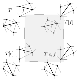
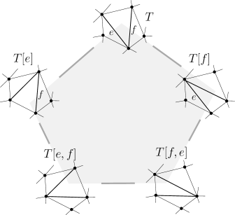
Figure 8: 4-Cycle $(T,T[e],T[e,f],T[f],T)$ and 5-cycle $(T,T[e],T[e,f],T[f,e],T[f],T)$ for $e$ and $f$ independently flippable and weakly independently flippable, respectively.

3.4 Proof of Lemma 3.1

Proof. Let $e$ and $f\neq e$ be flippable edges in $T$, i.e., $T[e]=T[\nicefrac{{e}}{{\overline{e}}}]$ and $T[f]=T[\nicefrac{{f}}{{\overline{f}}}]$ are defined for appropriate edges $\overline{e}$ and $\overline{f}$. Suppose the degree of $T[e]$ is at most the degree of $T[f]$. Our task is to identify, for each edge $g$ flippable in $T[e]$, a path $(T[e],T[e,g],\ldots,T[f,g^{*}],T[f])$, with these paths required to be vertex-disjoint. For this we distinguish four cases, depending on $g$.

1. $g=\overline{e}$: $(T[e],T,T[f])$ (note $T=T[e,\overline{e}]$).

2. $g=f$, if $f$ is flippable in $T[e]$: $(T[e],T[e,f],T[f])$ or $(T[e],T[e,f],T[f,e],T[f])$.

3. $g$ is flippable in $T[e]$, $T$, and $T[f]$: $(T[e],\!\!\begin{array}[]{c}T[e,g]\mbox{~{}or}\\ T[e,g],T[g,e]\end{array}\!\!,T[g],\!\!\begin{array}[]{c}T[g,f]\mbox{~{}or}\\ T[g,f],T[f,g]\end{array}\!\!,T[f])~{}.$

4. We still miss the paths $(T[e],T[e,g],\ldots)$ for edges $g\not\in\{\overline{e},f\}$ flippable in $T[e]$ but not flippable in $T$ or not flippable in $T[f]$. There are at most $8$ such edges $g$, since for this to happen, $g$ must be an edge of ${\sf terr}_{T}\hskip 1.00006pte={\sf terr}_{T[e]}\hskip 1.00006pt\overline{e}$ or of ${\sf terr}_{T}\hskip 1.00006ptf$. For such an edge $g$ choose an edge $g^{*}\not\in\{\overline{f},e\}$ flippable in $T[f]$ but not flippable in $T$ or $T[e]$. Because of our degree condition, $g^{*}$ must exist. Note that $g$ may equal $g^{*}$, if $g$ is flippable in $T[f]$ but not in $T$. Now we choose edges $x$ and $y$ flippable in $T$ with the three sets

   $${\sf terr}_{T}\hskip 1.00006ptx,~{}{\sf terr}_{T}\hskip 1.00006pty,\mbox{~{}and~{}}{\sf terr}_{T}\hskip 1.00006pte\cup{\sf terr}_{T}\hskip 1.00006ptf\cup{\sf terr}_{T}\hskip 1.00006ptg\cup{\sf terr}_{T}\hskip 1.00006ptg^{*}$$

   pairwise disjoint. These conditions allow for the following path

   $$(T[e],T[e,g],T[e,g,x],T[e,g,x,y],T[e,x,y],T[x,y],$$

   $$T[f,x,y],T[f,g^{*}\!,x,y],T[f,g^{*}\!,x],T[f,g^{*}],T[f])~{}.$$

   Every $g$ in this final category is paired up with a different $g^{*}$ and a different pair $\{x,y\}$ is chosen for building such a $T[e]$-$T[f]$-path. $P$ large enough will allow us to do so, by Thm. 1.6 and since we have to deal only with at most a constant (at most $8$) such cases.

For vertex-disjointness, we define for $T^{\prime}$ an internal vertex on such a $T[e]$-$T[f]$-path the signature $(\mathrm{\sf E}T[e]\cap\mathrm{\sf E}T[f])\setminus\mathrm{\sf E}T^{\prime}$. The internal vertices of our long paths in (d) have signatures

$$(\{g\},\{g,x\},\{g,x,y\},\{x,y\},\{x,y\},$$

$$\{x,y\},\{g^{*}\!,x,y\},\{g^{*}\!,x\},\{g^{*}\})$$

while previous cases gave signatures (again of internal vertices)

$$\underbrace{(\emptyset)}_{\mathrm{(a)\,}g=\overline{e}},~{}\underbrace{(\emptyset)\mbox{\,or\,}(\emptyset,\emptyset)}_{\mathrm{(b)\,}g=f},\mbox{~{}or~{}}\underbrace{(\{g\},\{g\},\ldots,\{g\})}_{\mathrm{(c)\,}g\mathrm{\,compatible\,with\,}e\mathrm{\,and\,}f\mathrm{\,in\,}T}~{}.$$

The vertex-disjointness of these paths can be readily concluded from these sequences and the proof is completed.

The restriction “$P$ large enough” is essential in Lemma 3.1, see Fig. 9.

         

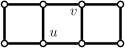
Figure 9: A edge flip graph with two vertices $u$ and $v$ of degree $3$ at distance $2$, which do not allow $3$ vertex-disjoint connecting paths.

3.5 Proof of Thm. 1.7(i)

Proof. The edge flip graph is connected and triangulations $T^{\prime}$ and $T^{\prime\prime}$ at distance $2$ in the edge flip graph can be written as $T^{\prime}=T[e]$ and $T^{\prime\prime}=T[f]$, for some $T\in{\cal T}_{\mathsf{full}}(P)$ and $e,f\in\mathrm{\sf E}T$. Therefore, Lemma 3.1 indeed implies Thm. 1.7(i) by the Local Menger Lemma 2.3.

As mentioned before, while “$P$ large enough” is essential in Lemma 3.1, we do not know whether it can be removed in Thm. 1.7(i).

4 Coarsening Full Subdivisions

In preparation of the proof of Thm. 1.7(ii), which will be presented in Sec. 5, we introduce full subdivisions of a point set, which form a partially ordered set under a relation we call refinement, and slack, a parameter of subdivisions. This will allow us to prove a lower bound on how many edges are compatible with a given flippable edge in a triangulation.

4.1 Full subdivisions

Definition 4.1 (full subdivision).

A full subdivision $S$ of $P$ is a connected plane graph with $\mathrm{\sf V}S=P$ and ${\sf E_{\mathsf{hull}}}\subseteq\mathrm{\sf E}S$, and all regions of $S$ convex.

Convention.

In Sec. 4 up to Sec. 6 we will use subdivision short for “full subdivision.”

Definition 4.2 (coarsening, refinement).

1. Given subdivisions $S_{1}$ and $S_{2}$ of $P$, we call $S_{1}$ a refinement of $S_{2}$, in symbols $S_{1}\preceq S_{2}$, if $\mathrm{\sf E}S_{1}\supseteq\mathrm{\sf E}S_{2}$ (or $S_{2}$ a coarsening of $S_{1}$, in symbols $S_{2}\succeq S_{1}$).

2. Given a subdivision $S$ of $P$, we let ${\cal T}_{\mathsf{full}}{\langle S\rangle}:=\{T\in{\cal T}_{\mathsf{full}}(P)\,|\,T\preceq S\}$, the set of triangulations of $P$ refining $S$.

Obviously, $\preceq$ is a partial order on subdivisions of $P$ with the triangulations the minimal elements. Note that if $S_{1}\preceq S_{2}$, then every region of $S_{1}$ is contained in some region of $S_{2}$, hence the name “refinement.” Here is a notion that allows us to identify edges in a subdivision that can be individually removed (not necessarily simultaneously removed) in order to obtain a coarsening.

  $\preceq$     $\preceq$  

Figure 10: A subdivision $S$, with edges directed to endpoints where they are locked. Edge $e$ is locked at both endpoints. Edges $f$, $f^{\prime}$, and $f^{\prime\prime}$ are not locked, each one can be removed obtaining a coarsening subdivision. Slacks of non-triangular regions are indicated (triangular regions have slack $0$). ${\sf sl}\hskip 1.00006ptS=2+1+1=4$. Removal of $f$ and $f^{\prime}$ yields a $\preceq$-maximal subdivision $S^{\prime}$ coarsening $S$. $T$ is a triangulation refining $S$.

Definition 4.3 (locked).

In a graph $G$ on $P$, an edge $e\in\mathrm{\sf E}G$ is locked at endpoint $p$ if the angle obtained at $p$ (between the edges adjacent to $e$ in radial order around $p$) after removal of $e$ is at least $\pi$ (in particular, if $p$ has degree $1$ or $2$ in $G$).

An edge in a triangulation is flippable iff it is not locked at any endpoint (in a triangulation, an edge can be locked at at most one of its endpoints). If $S$ is a subdivision, then removal of an edge $e$ in $S$ gives a subdivision iff $e$ is locked at none of its endpoints in $S$ (here, for a subdivision, an edge can be locked at both of its endpoints). Hence, the $\preceq$-maximal subdvisions are those with all of their edges locked.

Here are some simple fundamental properties of locking.

Observation 4.4.

Let $G$ be a graph on $P$ and $p\in\mathrm{\sf V}G$.

1. Any two edges locked at $p$ must be consecutive in the radial order around $p$.

2. There are at most $2$ edges locked at $p$, unless $p$ has degree $3$ in $G$.

3. If $G$ is a subdivision and $p\in P^{\circ}$ is of degree $3$, then the three edges incident to $p$ are locked at $p$.

Definition 4.5 (slack, refined slack).

Let $r$ be a region of a subdivision $S$, a convex set bounded by a $k$-gon, $k\geq 3$. Then we define the slack, ${\sf sl}\hskip 1.00006ptr$, of $r$ as $k-3$, and the refined slack, ${\sf sl^{*}}r$, of $r$ as $\lceil\frac{{\sf sl}\hskip 0.70004ptr}{2}\rceil$.

The slack, ${\sf sl}\hskip 1.00006ptS$, of subdivision $S$ is the sum of the slacks of its regions. The refined slack, ${\sf sl^{*}}S$, is the sum of the refined slacks of its regions.

Note that $k-3$ is the number of edges it takes to triangulate a $k$-gon. Hence, the slack of a subdivision is the number of edges which have to be added towards a triangulation. We need the following well-known facts on the number of edges and regions of triangulations.

Lemma 4.6.

For $T\in{\cal T}_{\mathsf{full}}(P)$, the number of edges, $|\mathrm{\sf E}T|$, equals $|\mathrm{\sf E^{\circ}}T|+h=3n-3-h=3n^{\!\circ}-3+2h$ and the number of regions, $|\mathrm{\sf R}T|$, equals $2n-2-h=2n^{\!\circ}-2+h$ (recall that the unbounded face is not a region).

Observation 4.7.

For a subdivision $S$, we have

$${\sf sl}\hskip 1.00006ptS = 3n-3-h-|\mathrm{\sf E}S|=3n^{\circ}-3+h-|\mathrm{\sf E^{\circ}}S|\mbox{~{},~{}and}$$

$$= 2n-2-h-|\mathrm{\sf R}S|=2n^{\circ}-2+h-|\mathrm{\sf R}S|~{}.$$

4.2 Unoriented Edges Lemma

Definition 4.8.

Let $\vec{G}$ be a graph $G$ on $P$ with some of its edges oriented to one of its endpoints and some edges unoriented; we call this a partially oriented graph. $\vec{G}$ is well-oriented if (a) no edge is directed to a point in ${\sf xtr}P$, and (b) if edges $e$ and $f$ are directed to a common point $p$, then $e$ and $f$ have to be consecutive in radial order around $p$.

Suppose, given a subdivision, we orient each locked inner edge to one locking endpoint (and we leave all other edges, in particular the boundary edges, unoriented), then Obs. 4.4 shows that this is a well-oriented graph. This is how we will employ the following lemma.

Lemma 4.9 (Unoriented Edges Lemma).

Let $\vec{S}$ be a partially oriented subdivsion of $P$. Let $C_{i}$, $i\in\mathbb{N}_{0}$, be the number of inner points of $\vec{S}$ with indegree $i$ and let $D:={\sf sl}\hskip 1.00006ptS$ and $D^{*}:={\sf sl^{*}}S$.

1. If $C_{i}=0$ for $i\geq 4$ then the number of unoriented inner edges equals

   $$n-3-C_{3}-D+(C_{1}+2C_{0})\geq n-3-C_{3}-D\geq h-3-D~{}.$$

2. Suppose $\vec{S}$ is well-oriented. Then the number of unoriented inner edges is at least

   $$\frac{n}{2}-2-\frac{D+D^{*}}{2}\geq\frac{n}{2}-2-D~{}.$$ (3)

Proof. (i) $n^{\!\circ}=C_{3}+C_{2}+C_{1}+C_{0}$ since $C_{i}=0$ for $i\geq 4$. $|\mathrm{\sf E^{\circ}}S|=3n^{\!\circ}-3+h-D$ (Obs. 4.7). Since $\vec{S}$ has $3C_{3}+2C_{2}+C_{1}$ oriented edges, the number of unoriented inner edges is

$$\underbrace{3n^{\!\circ}-3+h}_{=n-3+2(C_{3}+C_{2}+C_{1}+C_{0})}-D-(3C_{3}+2C_{2}+C_{1}) = n-3-C_{3}-D+C_{1}+2C_{0}$$

$$\geq n-3-C_{3}-D$$

$$\geq h-3-D\mbox{\hskip 43.05542pt since $C_{3}\leq n-h$.}$$

(ii) Let every inner point charge $1$ to each region incident to it that lies between two incoming edges. The overall charge made is exactly $3C_{3}+C_{2}$ (if the indegree is $3$, the degree is $3$; if the indegree is $2$, the two incoming edges are consecutive). While each triangular region can be charged at most once, other regions can be multiply charged: A region with slack $d$, a $(d+3)$-gon, is charged at most $\lfloor\frac{d+3}{2}\rfloor=1+\lfloor\frac{d+1}{2}\rfloor=1+\lceil\frac{d}{2}\rceil$ times (vertices charging a region $r$ cannot be consecutive along the boundary of $r$). Hence, if $\ell$ is the number of regions charged at all, the overall charge made to these $\ell$ regions is at most $\ell+D^{*}$. Thus $3C_{3}+C_{2}\leq\ell+D^{*}$, i.e., $\ell$ is at least $3C_{3}+C_{2}-D^{*}$. Moreover, $\ell$ is at most $2n^{\!\circ}-2+h-D$, the overall number of regions (Obs. 4.7). That is,

$$3C_{3}+C_{2}-D^{*}\leq 2n^{\!\circ}-2+h-D=\underbrace{n^{\!\circ}+h}_{=n}-2+\overbrace{C_{3}+C_{2}+C_{1}+C_{0}}^{n^{\!\circ}=}-D$$

$$\Leftrightarrow C_{3}\leq\frac{n}{2}-1-\frac{D-D^{*}}{2}+\frac{C_{0}+C_{1}}{2}$$

We plug this bound on $C_{3}$ into the number of unoriented edges derived in (4.2) above:

$$n-3-C_{3}-D+C_{1}+2C_{0}$$

$$\geq n-3-\frac{n}{2}+1+\frac{D-D^{*}}{2}-\frac{C_{0}+C_{1}}{2}-D+C_{1}+2C_{0}$$

$$= \frac{n}{2}-2-\frac{D+D^{*}}{2}+\frac{C_{1}+3C_{0}}{2}$$

The left bound in (ii) on the number of unoriented follows readily. Moreover, $\left\lceil\frac{d}{2}\right\rceil\leq d$ for $d\in\mathbb{N}_{0}$, hence $D^{*}\leq D$, i.e., $\frac{D+D^{*}}{2}\leq D$ and the right bound in (ii) is implied.

Lemma 4.10 (Coarsening Lemma for full subdivisions).

Any $\preceq$-maximal subdivision $S$ of $P$ (i.e., all edges in $\mathrm{\sf E^{\circ}}S$ are locked) has slack at least $\max\{\frac{n}{2}-2,h-3\}$.

Proof. Orient each edge in $S$ to a locking endpoint (ties broken arbitrarily). This gives a well-oriented graph $\vec{S}$ without unoriented inner edges. Since Lemma 4.9(i) and (ii) guarantees at least $\max\{h-3-{\sf sl}\hskip 1.00006ptS,\frac{n}{2}-2-{\sf sl}\hskip 1.00006ptS\}$ unoriented inner edges, we have $\max\{\frac{n}{2}-2,h-3\}-{\sf sl}\hskip 1.00006ptS\leq 0$.

Here is the essential implication on the number of compatible edges.

Corollary 4.11.

1. Every $T\in{\cal T}_{\mathsf{full}}(P)$ has at least $\max\{\frac{n}{2}-2,h-3\}$ flippable edges.

2. Given $T\in{\cal T}_{\mathsf{full}}(P)$ and $e$ flippable in $T$, there are at least $\max\{\frac{n}{2}-3,h-4\}$ edges in $\mathrm{\sf E}T$ compatible with $e$.

Proof. (i) Let $S$ be a $\preceq$-maximal subdivision with $S\succeq T$. Then all edges in $\mathrm{\sf E}T\setminus\mathrm{\sf E}S$ are flippable in $T$. Since $|\mathrm{\sf E}T\setminus\mathrm{\sf E}S|={\sf sl}\hskip 1.00006ptS$, the claim follows by Lemma 4.10.

(ii) Let $T_{-e}$ be the graph obtained by removing the edge $e$ from $T$. Since $e$ is flippable, $T_{-e}$ is a subdivision. Let $S$ be a $\preceq$-maximal coarsening of $T_{-e}$. All edges in $\mathrm{\sf E}T_{-e}\setminus\mathrm{\sf E}S$ are compatible with $e$ in $T$. Since $|\mathrm{\sf E}T_{-e}\setminus\mathrm{\sf E}S|={\sf sl}\hskip 1.00006ptS-1$, the claim follows again by Lemma 4.10.

We see that Cor. 4.11(i) is Thm. 1.6 by Hurtado et al. [22]. Actually, the set $\mathrm{\sf E}T\setminus\mathrm{\sf E}S$ in the argument for Cor. 4.11(i) is what is called ps-flippable (pseudo-simultaneously flippable) by Hoffmann et al. [20], where a lower bound of $\max\{\frac{n}{2}-2,h-3\}$ is shown for such ps-flippable edges. The proof (not the statement) of [20, Lemma 1.3] implies Lemma 4.10 above. We want to claim that the proof given above, including the proof of the Unoriented Edges Lemma 4.9 employed, is more concise. We emphasize, though, that our proof of the Unoriented Edges Lemma and its set-up is clearly inspired by the proof of the $\lceil\frac{n}{2}-2\rceil$-bound for flippable edges in [22] (see also [12] for Lemma 4.10(i)).

Here is another application of Lemma 4.10 which we mention here, although it will play no role in the rest of the paper. A set of pairwise independently flippable edges is often called simultaneously flippable in the literature. Here is a streamlined proof of the known tight lower bound on their number by Souvaine et al. from 2011, [35], based on the Unoriented Edges Lemma 4.9.

Theorem 4.12 ([35]).

Every triangulation $T$ of $P$ has a set of at least $\lceil\frac{n-4}{5}\rceil$ edges that are pairwise independently flippable (simultaneously flippable).

Proof. Let $S$ be a $\preceq$-maximal coarsening of $T$. Orient edges in $S$ (all locked) to a locking endpoint (ties broken arbitrarily). Lemma 4.9(ii) guarantees at least $\frac{n-4-({\sf sl}\hskip 0.70004ptS+{\sf sl^{*}}S)}{2}$ unoriented edges in $\vec{S}$. Since all inner edges are oriented, ${\sf sl}\hskip 1.00006ptS+{\sf sl^{*}}S\geq n-4$ holds.

For each region $r$ of $S$ of slack $d$, $T$ induces a triangulation of this $(d+3)$-gon. Its $d$ diagonals can be 3-colored with no triangle incident to two edges of the same color (start with an edge and spread the coloring along the dual tree of the triangulation of $r$). Each color class offers a set of simultaneously flippable edges, one of size at least $\lceil\frac{d}{3}\rceil$. It is easy to verify that $\left\lceil\frac{d}{3}\right\rceil\geq\frac{d+\lceil d/2\rceil}{5}$ (check for $d=0,1,2$; for $d\geq 3$, $\lceil\frac{d}{3}\rceil\geq\frac{d}{3}\geq\frac{d+(d+1)/2}{5}\geq\frac{d+\lceil d/2\rceil}{5}$). We combine the simultaneously flippable edges collected for each region of $S$, which gives an overall set of at least $\frac{{\sf sl}\hskip 0.70004ptS+{\sf sl^{*}}S}{5}\geq\frac{n-4}{5}$ simultaneously flippable edges.

While the lower bounds of $\frac{n-4}{2}$ for the number of flippable edges, and of $\frac{n-4}{5}$ for the size of a set of simultaneously flippable edges are tight (see [22] and [16], respectively), it is interesting to observe from the proofs that both bounds cannot be simultaneously attained for the same point set. That is, if the number of flippable edges is close to its lower bound then this forces the existence of a set of more than $\lceil\frac{n-4}{5}\rceil$ simultaneously flippable edges, and vice versa. This can be quantified as follows.

Theorem 4.13.

If the number of flippable edges in a triangulation $T$ of $P$ is $\alpha$, and if the largest set of simultaneously flippable edges in $T$ has size $\beta$, then $\alpha+\beta\geq\frac{4(n-4)}{5}$.

Proof. Let $S$ be a $\preceq$-maximal coarsening of $T$, with $d_{1}$, $d_{2}$, …, $d_{|\mathrm{\sf R}S|}$ the slacks of the regions of $S$. Then $\alpha\geq\sum_{i}d_{i}$ and, by the proof of Thm. 4.12, $\beta\geq\sum_{i}\lceil\frac{d_{i}}{3}\rceil$. Note that $d+\lceil\frac{d}{3}\rceil\geq\frac{4}{5}(d+\lceil d/2\rceil)$ for all $d\in\mathbb{N}_{0}$ (for $d=0,1,2$ we have $d+\lceil\frac{d}{3}\rceil=d+\lceil d/2\rceil$ and for $d\geq 3$, $d+\lceil\frac{d}{3}\rceil\geq\frac{4d}{3}\geq\frac{4(d+(d+1)/2)}{5}\geq\frac{4(d+\lceil d/2\rceil)}{5}$). Therefore, $\alpha+\beta\geq\frac{4({\sf sl}\hskip 0.70004ptS+{\sf sl^{*}}S)}{5}\geq\frac{4(n-4)}{5}$ (Lemma 4.9(ii)).

Let us conclude this section with an observation about interior-disjoint $k$-holes, as it emerged from a discussion with M. Scheucher (see also [34]). A $k$-hole of $P$ is a subset of $k$ points in convex position whose convex hull is disjoint from all other points in $P$. A $k$-hole and an $\ell$-hole are called interior-disjoint, if their respective convex hulls are interior-disjoint (they can share up to $2$ points). Harborth showed in 1978, [19], that every set of at least $10$ points has a $5$-hole. This was recently strengthened to the existence of another interior-disjoint $4$-hole, [21, Thm. 2]. We show, how our framework allows an easy proof of this fact.

Theorem 4.14 ([21]).

Every set $P$ of at least $10$ points has a $5$-hole and a $4$-hole which are interior-disjoint.

Proof. Since $P$ has a 5-hole, [19], there is a subdivision of $P$ with a region of slack $2$. Consider a $\preceq$-maximal coarsening $S$ of such a subdivision with $r$ a region of largest slack. We know that ${\sf sl}\hskip 1.00006ptr\geq 2$. If ${\sf sl}\hskip 1.00006ptr\geq 4$, i.e., it is a $k$-gon with $k\geq 7$, then we can add a diagonal to $r$ which divides $r$ into a $5$-gon and a $(k-3)$-gon which readily gives the claimed interior-disjoint holes. Otherwise, if $k\leq 6$, we have ${\sf sl}\hskip 1.00006ptr+{\sf sl^{*}}r\leq 5$, while ${\sf sl}\hskip 1.00006ptS+{\sf sl^{*}}S\geq n-4\geq 6$ (Lemma 4.9(ii)). Hence, there must be another region $r^{\prime}\in\mathrm{\sf R}S$ with positive slack, i.e., a $k^{\prime}$-gon with $k^{\prime}\geq 4$.

5 $\max\{\lceil\frac{n}{2}-2\rceil,h-3\}$-Bound for Full Triangulations

The proof of Thm. 1.7(ii) needs one more ingredient.

5.1 Link of a full triangulation

The link of a triangulation is the graph representing the compatibility relation among its flippable edges. In Sec. 1.7, the intuition for links as counterparts of vertex figures in polytopes was briefly explained.

Definition 5.1 (link of full triangulation).

For $T\in{\cal T}_{\mathsf{full}}(P)$, the link of $T$, denoted ${\mathsf{Lk}}_{\mathsf{full}}T$, is the edge-weighted graph with vertices $\mathrm{\sf F}T:=\{e\in\mathrm{\sf E^{\circ}}T\mid e\mbox{~{}flippable~{}in~{}}T\}$ and edge set $\{\{e,f\}\in{\mathrm{\sf F}T\choose 2}\mid e\mbox{~{}and~{}}f\mbox{~{}compatible}\}$. The weight of an edge $\{e,f\}$ is $2$ if $e$ and $f$ are independently flippable, and $3$ if $e$ and $f$ are weakly independently flippable.

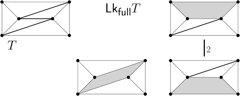
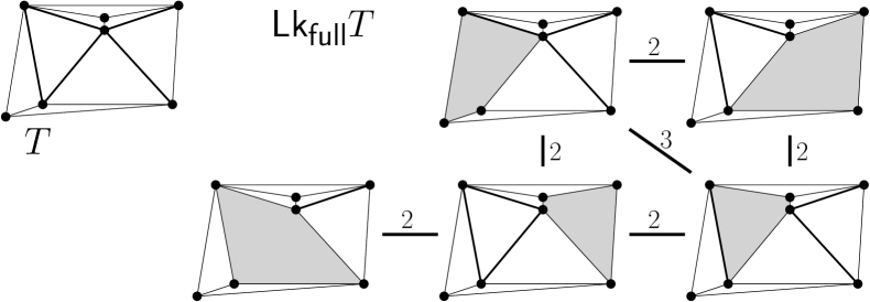
Figure 11: Two examples of links, the left link has $3$ vertices, one of which is isolated. We indicate vertices of the link, i.e., $e\in\mathrm{\sf F}T$, also as $T[e]=T[\nicefrac{{e}}{{\overline{e}}}]$ with ${\sf terr}_{T}\hskip 1.00006pte={\sf terr}_{T[e]}\hskip 1.00006pt\overline{e}$ shaded. Small examples are not typical: For large sets, the link is a dense highly connected graph.

We will see that for proving Thm. 1.7(ii) (in Sec. 5.2 below) it is enough to prove $\lceil\frac{n}{2}-3\rceil$-vertex connectivity of links. Here is the special property of links that will immediately show that the vertex connectivity is determined by the minimum vertex degree (via Lemma 2.4).

Lemma 5.2.

For $T\in{\cal T}_{\mathsf{full}}(P)$, the complement of ${\mathsf{Lk}}_{\mathsf{full}}T$ has no cycle of length $4$, i.e., if $(e_{0},e_{1},e_{2},e_{3})$ are flippable edges in $T$, then there exists $i\in\{0,1,2,3\}$ such that $e_{i}$ is compatible with $e_{i+1\!\bmod\!4}$.

Proof. For $e$ and $f$ flippable edges in $T$ we show that there is at most one flippable edge $g$ that is compatible with neither $e$ nor $f$; this implies the lemma. Such a $g$ has to be an edge of both ${\sf terr}\hskip 1.00006pte$ and ${\sf terr}\hskip 1.00006ptf$. If ${\sf terr}\hskip 1.00006pte$ and ${\sf terr}\hskip 1.00006ptf$ are disjoint, they share at most one edge (since ${\sf terr}\hskip 1.00006pte$ and ${\sf terr}\hskip 1.00006ptf$ are convex, see Fig. 12 (left). Otherwise, ${\sf terr}\hskip 1.00006pte$ and ${\sf terr}\hskip 1.00006ptf$ overlap in a triangle $\Delta$, of which $e$ and $f$ are edges; the third edge $g$ of this triangle is the a common edge of ${\sf terr}\hskip 1.00006pte$ and ${\sf terr}\hskip 1.00006ptf$, see Fig. 12 (right). No other edge of ${\sf terr}\hskip 1.00006ptf$ can appear on the boundary of ${\sf terr}\hskip 1.00006pte$: Consider the line $\lambda$ through edge $f$. All edges of ${\sf terr}\hskip 1.00006ptf$ other than $e$ and $g$ lie on the side of $\lambda$ opposite to $\Delta$, and ${\sf terr}\hskip 1.00006pte$ is on the same side of $\lambda$ as $\Delta$, since it contains $\Delta$ and $f$ is an edge of ${\sf terr}\hskip 1.00006pte$; again, convexity of ${\sf terr}\hskip 1.00006pte$ and of ${\sf terr}\hskip 1.00006ptf$ is essential here.

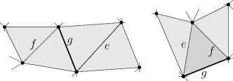
Figure 12: Edge $g$ in the intersection of boundaries of territories of flippable edges $e$ and $f$.

Lemma 5.3.

For $T\in{\cal T}_{\mathsf{full}}(P)$, the link ${\mathsf{Lk}}_{\mathsf{full}}T$ is $\max\{\lceil\frac{n}{2}-3\rceil,h-4\}$-vertex connected.

Proof. Every flippable edge in $T$ is compatible with at least $\max\{\lceil\frac{n}{2}-3\rceil,h-4\}$ edges (Cor. 4.11(ii)), i.e., the minimum vertex degree in ${\mathsf{Lk}}_{\mathsf{full}}T$ is at least $\max\{\lceil\frac{n}{2}-3\rceil,h-4\}$. ${\mathsf{Lk}}_{\mathsf{full}}T$ has no cycle of length $4$ in its complement (Lemma 5.2). The lemma follows (Lemma 2.4).

Lemma 5.4.

Given flippable edges $e$ and $f$, $e\neq f$, in $T\in{\cal T}_{\mathsf{full}}(P)$, every $e$-$f$-path of weight $w$ in ${\mathsf{Lk}}_{\mathsf{full}}T$ induces a $T$-avoiding $T[e]$-$T[f]$-path of length $w$ in the edge flip graph, in a way that vertex-disjoint $e$-$f$-paths in the link induce vertex-disjoint $T[e]$-$T[f]$-paths.

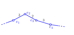
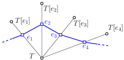
Figure 13: From a path in the link ${\mathsf{Lk}}_{\mathsf{full}}T$ to a path in the edge flip graph.

Proof. Given an $e$-$f$-path in ${\mathsf{Lk}}_{\mathsf{full}}T$, we replace each edge $\{z^{\prime},z^{\prime\prime}\}$ on this path (i.e., $z^{\prime}$ and $z^{\prime\prime}$ are compatible) by the path $(T[z^{\prime}],T[z^{\prime},z^{\prime\prime}],T[z^{\prime\prime}])$ or $(T[z^{\prime}],T[z^{\prime},z^{\prime\prime}],T[z^{\prime\prime},z^{\prime}],T[z^{\prime\prime}])$, depending on whether $z^{\prime}$ and $z^{\prime\prime}$ are independently flippable (weight of $\{z^{\prime},z^{\prime\prime}\}$ is $2$) or weakly independently flippable (weight of $\{z^{\prime},z^{\prime\prime}\}$ is $3$), respectively, see Lemma 3.7 (Fig. 13). Note that the vertices $T[z^{\prime},z^{\prime\prime}]$ and $T[z^{\prime\prime},z^{\prime}]$ at distance $2$ from $T$ (recall triangle-freeness, Cor. 3.4) on these substitutes satisfy $\mathrm{\sf E}T\setminus\mathrm{\sf E}T[z^{\prime},z^{\prime\prime}]=\mathrm{\sf E}T\setminus\mathrm{\sf E}T[z^{\prime\prime},z^{\prime}]=\{z^{\prime},z^{\prime\prime}\}$ (Lemma 3.3(ii)(2)). Therefore, these vertices cannot appear on any substitute for another edge on the given $e$-$f$-path, nor on substitutes for any other vertex-disjoint $e$-$f$-path. Clearly, also the internal vertices at distance $1$ from $T$ (i.e., of the form $T[z]$) are distinct from internal vertices at other vertex-disjoint $e$-$f$-paths. And, obviously, we have not employed the vertex $T$ for the substituting paths.

5.2 Proof of Thm. 1.7(ii)

Proof. We want to show that for $n\geq 5$, the edge flip graph is $\max\{\lceil\frac{n}{2}-2\rceil,h-3\}$-vertex connected. We employ the Local Menger Lemma 2.3. We know that the edge flip graph is connected, [23]. What is left to show is that for any triangulation $T\in{\cal T}_{\mathsf{full}}(P)$ and edges $e$ and $f$ flippable in $T$, at least $\max\{\lceil\frac{n}{2}-2\rceil,h-3\}$ vertex-disjoint $T[e]$-$T[f]$-paths exist in the edge flip graph. ${\mathsf{Lk}}_{\mathsf{full}}T$ has at least $\max\{\lceil\frac{n}{2}-3\rceil,h-4\}$ vertex-disjoint $e$-$f$-paths (Lemma 5.3 and Menger’s Theorem 2.2). Therefore, there are at least $\max\{\lceil\frac{n}{2}-3\rceil,h-4\}$ $T$-avoiding vertex-disjoint $T[e]$-$T[f]$-paths (Lemma 5.4). The extra path $(T[e],T,T[f])$ yields the theorem.

6 Covering the Edge Flip Graph with Polytopes

Recall from Sec. 1.3 that for a convex $k$-gon there is a $(k-3)$-polytope whose 1-skeleton is isomorphic to the edge flip graph of triangulations of the $k$-gon, an associahedron, which we denote by ${\cal A}_{k-3}$ (the index reflecting its dimension); ${\cal A}_{1}$ is an edge, ${\cal A}_{2}$ is a convex pentagon, etc. If we consider all triangulations of the $k$-gon with a given diagonal present, we get a facet of ${\cal A}_{k-3}$; all facets of ${\cal A}_{k-3}$ can be obtained in this way. In general, the $d$-faces of ${\cal A}_{k-3}$ represent the triangulations where a certain set of $k-3-d$ diagonals is present, i.e., a subdivision.

                   

Figure 14: 3-dimensional products of associahedra for subdivisions of slack $3$: ${\cal A}_{1,2}$ (a pentagonal prism), ${\cal A}_{1,1,1}$ (a cube), and ${\cal A}_{3}$.

Suppose now that we have a subdivision $S$ of $P$ with nontriangular regions $r_{1},r_{2},\ldots,r_{m}$, with $r_{i}$ of slack $d_{i}$. Then the set, ${\cal T}_{\mathsf{full}}{\langle S\rangle}$, triangulations refining $S$, with its edge flip graph is represented by the product (see [39])

$${\cal A}_{d_{1},d_{2},\ldots,d_{m}}:={\cal A}_{d_{1}}\times{\cal A}_{d_{2}}\times\cdots\times{\cal A}_{d_{m}}~{},$$

a $d$-dimensional polytope for $d:=d_{1}+d_{2}+\ldots+d_{m}={\sf sl}\hskip 1.00006ptS$.

It is now easy to see that any edge of the edge flip graph finds itself in the 1-skeleton of such a $\max\{\lceil\frac{n}{2}-2\rceil,h-3\}$-dimensional polytope contained in the edge flip graph (see also the discussion in Sec. 1.5).

Theorem 6.1.

For every edge $\{T,T[e]\}$ of the edge flip graph  there is an induced subgraph of the edge flip graph which contains the edge $\{T,T[e]\}$ and is isomorphic to the 1-skeleton of a product ${\cal A}_{d_{1},d_{2},\ldots,d_{m}}$ of associahedra, where $d:=d_{1}+d_{2}+\cdots+d_{m}\geq\max\{\lceil\frac{n}{2}-2\rceil,h-3\}$. Therefore, the edge flip graph (vertices and edges) can be covered by $1$-skeletons of $\max\{\lceil\frac{n}{2}-2\rceil,h-3\}$-dimensional products of associahedra contained in the edge flip graph.

Proof. Let $S$ a $\preceq$-maximal coarsening of the subdivision $T_{-e}$ ($T$ with $e$ removed). Then ${\sf sl}\hskip 1.00006ptS\geq\max\{\lceil\frac{n}{2}-2\rceil,h-3\}$ holds (Coarsening Lemma 4.10). The subgraph induced by ${\cal T}_{\mathsf{full}}{\langle S\rangle}$ gives the claimed product of associahedra.

One can strengthen this and show that any pair of incident edges in the edge flip graph is part of a subgraph isomorphic to the 1-skeleton of some $\lceil\frac{n}{2}-2\rceil$-dimensional polytope (a glueing of products of associahedra). This has been discussed in [37], but we decided to skip that part in this version.

7 Partial Subdivisions – Slack and Order

In Sections 7-9 we move on to proving Thm. 1.9, the $(n-3)$-vertex connectivity for the bistellar flip graph of partial triangulations. As indicated in the introduction, the proof will follow a similar line as for the edge flip graph, using subdivisions and links, but several new aspects and challenges will appear.

Convention.

From now on, in Sections 7-11, we will mostly use triangulation short for “partial triangulation,” but we return to using “full triangulation” and “full subdivision.”

We define partial subdivisions, which form a poset in which the triangulations of $P$ are the minimal elements – our definition is a specialization, to the plane and general position, of the established notion of a polyhedral subdivision, [11]. These partial subdivisions are plane graphs, possibly with isolated points. Hence, it may be useful to point out a subtlety in the definition of regions of a plane graph (Def. 1.2): We defined them as the bounded connected components in the complement of the union the edges (as line segments in $\mathbb{R}^{2}$), not taking the isolated points into account. That is, regions can contain isolated points of the graph, and isolated points will not keep them from being convex.

Definition 7.1 (partial subdivision).

A partial subdivision $S$ of $P$ is a graph with $\mathrm{\sf V}S\subseteq P$ and ${\sf E_{\mathsf{hull}}}(P)\subseteq\mathrm{\sf E}S$ (hence ${\sf xtr}P\subseteq\mathrm{\sf V}S$), and with all of its regions convex.

Similar to triangulations (Def. 1.3), we define $\mathrm{\sf E^{\circ}}S:=\mathrm{\sf E}S\setminus{\sf E_{\mathsf{hull}}}$ (the inner edges of $S$) and $\mathrm{\sf V^{\circ}}S:=\mathrm{\sf V}S\cap P^{\circ}$ (the inner points of $S$). Moreover, we let $\mathrm{\sf V^{by}}S$ be the points in $\mathrm{\sf V}S$ which are isolated in $S$, the bystanders of $S$, and we let $\mathrm{\sf V^{inv}}S:=\mathrm{\sf V^{\circ}}S\setminus\mathrm{\sf V^{by}}S$, the involved points of $S$.

For a region $r$ of $S$, let $\mathrm{\sf V}r:=\overline{r}\cap\mathrm{\sf V}S$ ($\overline{r}$ the closure of $r$), i.e., these are the vertices of the convex polygon $r$ and the bystanders in this region.

$\mathsf{S}_{\mathsf{triv}}=\mathsf{S}_{\mathsf{triv}}(P):=(P,{\sf E_{\mathsf{hull}}})$ is called the trivial subdivision of $P$.

Observe that a partial subdivision $S$ is a full subdivision of $P$ iff $\mathrm{\sf V}S=P$ and $\mathrm{\sf V^{by}}S=\emptyset$. Also, a partial subdivision $S$ is a full subdivision of $\mathrm{\sf V}S\setminus\mathrm{\sf V^{by}}S$.

         

Figure 15: A set $P$ and a partial subdivisions $S$ of $P$. Crosses indicate skipped points. Points $p$ and $q$ are bystanders. The region containing $p$ has slack $6-3=3$ (Def. 7.2 below).

Convention.

From now on, in Sections 7-11, we will mostly use subdivision for “partial subdivision.”

As it should have become clear by now, $\mathrm{\sf V}S$ is essential in the definition of a subdivision $S$, it is not simply the set of endpoints of edges in $S$, there are also bystanders. For example, for $T\in{\cal T}_{\mathsf{part}}(P)$, all graphs $(P^{\prime},\mathrm{\sf E}T)$ with $\mathrm{\sf V}T\subseteq P^{\prime}\subseteq P$ are subdivisions of $P$, all different. $\mathrm{\sf V}S$ partitions into boundary points, involved points, and bystanders, i.e., $\mathrm{\sf V}S={\sf xtr}P\,\dot{\cup}\,\mathrm{\sf V^{inv}}S\,\dot{\cup}\,\mathrm{\sf V^{by}}S$. Moreover, there are the skipped points, $P\setminus\mathrm{\sf V}S=P^{\circ}\setminus\mathrm{\sf V^{\circ}}S$.

A first important example of a subdivision is obtained from a triangulation $T$ and an element $x$ flippable in $T$, i.e., $\{T,T[x]\}$ is an edge of the bistellar flip graph:

$$T_{\pm x}:=(\mathrm{\sf V}T\cup\mathrm{\sf V}T[x],\mathrm{\sf E}T\cap\mathrm{\sf E}T[x])$$

If $x=e$ is a flippable edge, then $T_{\pm e}$ has one convex quadrilateral region $Q$; all other regions are triangular. We obtain $T$ and $T[e]$ from $T_{\pm e}$ by adding one or the other of the 2 diagonals of $Q$ to $T_{\pm e}$. If $x=p$ is a flippable point, then $T_{\pm p}$ is almost a triangulation, all regions are triangular, except that $p\in\mathrm{\sf V}T_{\pm p}$ is a bystander. We obtain $T$ and $T[p]$ by either removing this point from $T_{\pm p}$ or by adding the three edges from $p$ to the points of the triangular region in which $p$ lies. The subdivision $T_{\pm x}$ is close to a triangulation and, in a sense, represents the flip between $T$ and $T[x]$. To formalize and generalize this we generalize the notion of slack from full to partial subdivisions.

Definition 7.2 (slack of partial subdivision).

Given a subdivision $S$ of $P$, we call a region of $S$ active if it is not triangular or if it contains at least one point in $\mathrm{\sf V}S$ (necessarily a bystander) in its interior.

For $r\in\mathrm{\sf R}S$, the slack, ${\sf sl}\hskip 1.00006ptr$, of $r$ is $|\mathrm{\sf V}r|-3$. The slack of $S$, ${\sf sl}\hskip 1.00006ptS$, is the sum of slacks of its regions.

Note that a region is active iff it has nonzero slack.

Observation 7.3.

For a subdivision $S$ with $s$ bystanders we have

$${\sf sl}\hskip 1.00006ptS=3(|\mathrm{\sf V}S|-s)-3-h-|\mathrm{\sf E}S|+s=3|\mathrm{\sf V}S|-3-h-|\mathrm{\sf E}S|-2s~{}.$$

Proof. The slack of a region $r$ equals the number of edges it takes to triangulate $r$ (ignoring bystanders) plus the number of bystanders in $r$. Thus, ${\sf sl}\hskip 1.00006ptS$ is the number of edges it takes to triangulate $(\mathrm{\sf V}S\setminus\mathrm{\sf V^{by}}S,\mathrm{\sf E}S)$ (a full subdivision of $\mathrm{\sf V}S\setminus\mathrm{\sf V^{by}}S$) plus $|\mathrm{\sf V^{by}}S|$. Now the claim follows from Lemma 4.6 (or Obs. 4.7).

Observation 7.4.

Let $S$ be a subdivision.

1. ${\sf sl}\hskip 1.00006ptS=0$ iff $S$ is a triangulation iff $S$ has no active region.

2. ${\sf sl}\hskip 1.00006ptS=1$ iff $S$ has exactly one active region of slack $1$; this region is either a convex quadrilateral, or a triangular region with one bystander in its interior.

3. ${\sf sl}\hskip 1.00006ptS=2$ iff $S$ has either (a) exactly two active regions, both of slack $1$, or (b) exactly one active region of slack $2$, where this region is either a convex pentagon, or a convex quadrilateral with one bystander in its interior, or a triangular region with two bystanders in its interior.

Figure 16: Hasse diagram of the partial order $\preceq$ for a set of $5$ points.

Definition 7.5 (coarsening, refinement).

For subdivisions $S_{1}$ and $S_{2}$ of $P$, $S_{2}$ coarsens $S_{1}$, in symbols $S_{2}\succeq S_{1}$, if $\mathrm{\sf V}S_{2}\supseteq\mathrm{\sf V}S_{1}$, and $\mathrm{\sf E}S_{2}\subseteq\mathrm{\sf E}S_{1}$. We also say that $S_{1}$ refines $S_{2}$, ($S_{1}\preceq S_{2}$).

The example in Fig. 16 hides some of the intricacies of the partial order $\preceq$; e.g., in general, it is not true that all paths from a triangulation to $\mathsf{S}_{\mathsf{triv}}$ have the same length $n-3$. $\mathsf{S}_{\mathsf{triv}}$ is the unique coarsest ($\preceq$-maximal) element (quite contrary to the poset of full subdivisions, where there were several $\preceq$-maximal full subdivisions). The triangulations (i.e., subdivisions of slack $0$) are the minimal elements.

Definition 7.6 (set of refining partial triangulations).

For a subdivision $S$ of $P$ we let ${\cal T}_{\mathsf{part}}{\langle S\rangle}:=\{T\in{\cal T}_{\mathsf{part}}(P)\,|\,T\preceq S\}$.

Note that ${\cal T}_{\mathsf{part}}{\langle\mathsf{S}_{\mathsf{triv}}\rangle}={\cal T}_{\mathsf{part}}(P)$ and for $x$ flippable in $T$, ${\cal T}_{\mathsf{part}}{\langle T_{\pm x}\rangle}=\{T,T[x]\}$.

Observation 7.7.

(i) Any subdivision $S$ of slack $1$ of $P$ equals $T_{\pm x}$ for some triangulation $T\preceq S$ and some $x$ flippable in $T$. (ii) Let $S$ be a subdivision of slack $2$ of $P$. If there are exactly 2 active regions in $S$ (of slack $1$ each), then ${\cal T}_{\mathsf{part}}{\langle S\rangle}$ has cardinality $4$, spanning a $4$-cycle in the bistellar flip graph of $P$ (Fig. 17). If there is exactly one active region in $S$ (of slack $2$), then ${\cal T}_{\mathsf{part}}{\langle S\rangle}$ has cardinality $5$, spanning a $5$-cycle (see Fig. 2).

         

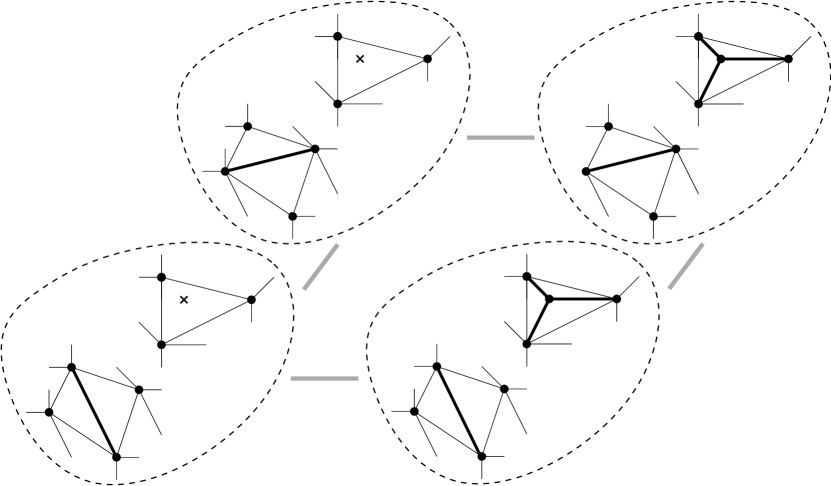
Figure 17: A subdivision $S$ with two active regions of slack $1$ each. ${\cal T}_{\mathsf{part}}{\langle S\rangle}$ spans a $4$-cycle in the bistellar flip graph.

Lemma 7.8.

Any proper refinement $S$ of a subdivision $S^{\prime}$ of slack $2$ has slack at most $1$.

Proof. For a refinement of $S^{\prime}$ we add $m$ edges, thereby involving $s^{\prime}$ bystanders, and we remove $s^{\prime\prime}$ bystanders (some of these parameters may be $0$, but not all, since the refinement is assumed to be proper). We have ${\sf sl}\hskip 1.00006ptS={\sf sl}\hskip 1.00006ptS^{\prime}-(m-2s^{\prime}+s^{\prime\prime})$ (easy consequence of Obs. 7.3) and we want to show $m-2s^{\prime}+s^{\prime\prime}>0$.

Since ${\sf sl}\hskip 1.00006ptS^{\prime}=2$, $S^{\prime}$ has at most two bystanders and thus $s^{\prime}\leq 2$. If $s^{\prime}=0$, then $m-2s^{\prime}+s^{\prime\prime}>0$ holds, since some of the three parameters have to be positive. If $s^{\prime}=1$, we observe that we need at least $3$ edges to involve a bystander and $m-2s^{\prime}\geq 3-2\cdot 1=1$. If $s^{\prime}=2$, we need at least $5$ edges to involve two bystanders and $m-2s^{\prime}\geq 5-2\cdot 2=1$.

For $D\geq 3$, a proper refinement of a subdivision of slack $D$ can have slack $D$ or even higher (Fig. 18). The proof fails, since we can involve $3$ bystanders with $6$ edges.

Figure 18: $8$ points, with a subdivision of slack $6$, a refinement of $\mathsf{S}_{\mathsf{triv}}$ of slack $8-3=5$.

Intuitively, as briefly alluded to at the end of Sec. 1.3 (for the special case of convex position), one can think of the subdivisions as the faces of a higher-dimensional geometric structure behind the bistellar flip graph, with slack playing the role of dimension, analogous to the secondary polytope for regular triangulations. The following lemma shows that – for slack at most $2$ – we have the property corresponding to the fact that faces of dimension $d$ are either equal, or intersect in a common face of smaller dimension (possibly empty). This correspondence fails for slack exceeding $2$.

Lemma 7.9.

1. For subdivisions $S_{1}$ and $S_{2}$ of slack $2$, ${\cal T}_{\mathsf{part}}{\langle S_{1}\rangle}\cap{\cal T}_{\mathsf{part}}{\langle S_{2}\rangle}$ is either (a) empty, (b) equals $\{T\}$ for some triangulation $T$, (c) equals $\{T,T[x]\}$ for some triangulation $T$ and some flippable element $x$, or (d) $S_{1}=S_{2}$.

2. Let $x$ and $y$ be two distinct flippable elements in triangulation $T$. If there is a subdivision $S$ of slack $2$ with $\{T[x],T,T[y]\}\subseteq{\cal T}_{\mathsf{part}}{\langle S\rangle}$, then this $S$ is unique.

Proof. If ${\cal T}_{\mathsf{part}}{\langle S_{1}\rangle}\cap{\cal T}_{\mathsf{part}}{\langle S_{2}\rangle}$ contains some triangulation, then we easily see that $S_{1}\wedge S_{2}:=(\mathrm{\sf V}S_{1}\cap\mathrm{\sf V}S_{2},\mathrm{\sf E}S_{1}\cup\mathrm{\sf E}S_{2})$ is a subdivision, and ${\cal T}_{\mathsf{part}}{\langle S_{1}\wedge S_{2}\rangle}={\cal T}_{\mathsf{part}}{\langle S_{1}\rangle}\cap{\cal T}_{\mathsf{part}}{\langle S_{2}\rangle}$.

(i) If (a) does not apply, let $S:=S_{1}\wedge S_{2}$, a subdivision with ${\cal T}_{\mathsf{part}}{\langle S\rangle}={\cal T}_{\mathsf{part}}{\langle S_{1}\rangle}\cap{\cal T}_{\mathsf{part}}{\langle S_{2}\rangle}$. If ${\sf sl}\hskip 1.00006ptS=0$ we have property (b), if ${\sf sl}\hskip 1.00006ptS=1$ we have property (c). In the remaining case ${\sf sl}\hskip 1.00006ptS\geq 2$, $S$ is a refinement of $S_{1}$ and of $S_{2}$. Lemma 7.8 tells us that $S$ cannot be a proper refinement of $S_{1}$, hence $S=S_{1}$; similarly, $S=S_{2}$, hence $S_{1}=S_{2}$.

(ii) Suppose $S_{1}$ and $S_{2}$ are subdivisions of slack $2$ with $\{T[x],T,T[y]\}\subseteq{\cal T}_{\mathsf{part}}{\langle S_{1}\rangle}\cap{\cal T}_{\mathsf{part}}{\langle S_{2}\rangle}$. Since options (a-c) above cannot apply, we are left with $S_{1}=S_{2}$.

Two edges incident to a vertex of a polytope may span a $2$-face, or not; same here, which gives rise to the following definition:

Definition 7.10 (compatible elements).

Two distinct flippable elements $x,y\in\mathrm{\sf V^{\circ}}T\cup\mathrm{\sf E^{\circ}}T$ are called compatible in $T$, in symbols $x\diamond y$, if there is a subdivision $T_{\pm x,y}\succeq T$ of slack $2$, s.t. $\{T[x],T,T[y]\}\subseteq{\cal T}_{\mathsf{part}}{\langle T_{\pm x,y}\rangle}$. (Note that $T_{\pm x,y}$ is unique, by Lemma 7.9(ii).) Otherwise, $x$ and $y$ are called incompatible in $T$, in symbols $x\mbox{$\not\!\diamond\,\,$}y$.

This needs some time to digest. In particular, if two flippable edges $e$ and $f$ share a common endpoint of degree $4$, then they are compatible (Fig. 19 bottom left), quite contrary to the situation for full triangulations as treated in Sec. 3.3 (see Def. 3.6). The configurations of 2 flippable but incompatible elements are shown in Fig. 19 (two rightmost): (a) Two flippable edges $e$ and $f$ whose removal creates a nonconvex pentagon and whose common endpoint $q$ has degree at least $5$. (b) A flippable edge $e$ and a flippable point $p$ of degree $3$ whose removal creates a nonconvex quadrilateral region whose reflex point $q$ has degree at least $5$ in the triangulation.

           

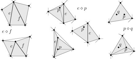
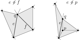
Figure 19: Compatible elements (with overlapping incident regions, all contained in a $5$-cycle, see Fig. 2, and incompatible elements (two rightmost, where $q$ is assumed to have degree at least $5$). Shaded areas are unions of incident regions of flippable elements (not the active region in $T_{\pm x,y}$!).

What is essential for us is that whenever $x$ and $y$ are compatible in a triangulation $T$, then there is a cycle of length $4$ or $5$ containing $(T[x],T,T[y])$, and therefore, apart from the path $(T[x],T,T[y])$, there exists a $T$-avoiding $T[x]$-$T[y]$-path of length $2$ or $3$.

Observation 7.11.

Let $T\in{\cal T}_{\mathsf{part}}(P)$. (i) A skipped point $p\in P^{\circ}\setminus\mathrm{\sf V^{\circ}}{T}$ is compatible with every flippable element of $T$. (ii) Any two flippable points $p,q\in P^{\circ}$ are compatible.

8 Coarsening Partial Subdivisions

As in Sections 4 and 5 for full triangulations, the existence of many coarsenings is essential for the vertex-connectivity of the bistellar flip graph. However, note right away that going via $\preceq$-maximal subdivisions – as for full subdivisions – will not work: Here, for partial subdivisions, there is a unique $\preceq$-maximal element, the trivial subdivision. Moreover, note that for full subdivisions (as employed in Sec. 4), if $S_{1}\preceq S_{2}$, then $(S_{1},S_{2})$ is an edge in the Hasse-diagram of the partial order $\preceq$ iff ${\sf sl}\hskip 1.00006ptS_{2}={\sf sl}\hskip 1.00006ptS_{1}+1$. For partial subdivisions, this is not the case (Fig. 20).

Figure 20: ${\sf sl}\hskip 1.00006ptS_{1}=2$, ${\sf sl}\hskip 1.00006ptS_{2}=3$, ${\sf sl}\hskip 1.00006ptS_{3}=3$. Note that $S_{2}\prec_{\mathrm{dir}}S_{3}$ but $S_{2}\not\prec_{1}S_{3}$, and that $S_{1}\preceq S_{3}$ with ${\sf sl}\hskip 1.00006ptS_{3}={\sf sl}\hskip 1.00006ptS_{1}+1$ but $S_{1}\not\prec_{1}S_{3}$.

Definition 8.1 (direct, perfect coarsening).

Let $S_{1}$ and $S_{2}$ be subdivisions. (i) We call $S_{2}$ a direct coarsening of $S_{1}$ (and $S_{1}$ a direct refinement of $S_{2}$), in symbols $S_{1}\prec_{\mathrm{dir}}S_{2}$, if $S_{1}\preceq S_{2}$ and any subdivision $S$ with $S_{1}\preceq S\preceq S_{2}$ satisfies $S\in\{S_{1},S_{2}\}$ (equivalently, if $(S_{1},S_{2})$ is an edge in the Hasse diagram of $\preceq$). (ii) We call $S_{2}$ a perfect coarsening of $S_{1}$ ($S_{1}$ a perfect refinement of $S_{2}$), in symbols $S_{1}\prec_{1}S_{2}$, if $S_{1}\prec_{\mathrm{dir}}S_{2}$ and ${\sf sl}\hskip 1.00006ptS_{2}={\sf sl}\hskip 1.00006ptS_{1}+1$. (iii) $\prec^{*}_{1}$ is the reflexive transitive closure of $\prec_{1}$.

The reflexive transitive closure of $\prec_{\mathrm{dir}}$ is exactly $\preceq$, while $\prec^{*}_{1}\,\subseteq\,\preceq$ and, in general, the inclusion is proper.

To motivate the upcoming definitions, let us discuss a few possibilities of coarsenings, direct coarsenings and perfect coarsenings. There are the simple operations of removing an unlocked edge, and of adding a skipped point $p\in P\setminus\mathrm{\sf V}S$ as a bystander. For a triangulation, we can isolate a point of degree $3$. How does this generalize to subdivisions? Removing the edges incident to a point of degree $3$ does not work if some incident edge might be locked at its other endpoint (e.g., $p_{0}$ in Fig. 21). If, however, no edge incident to a given point $p$ (of any degree) is locked at the respective other endpoint, then we can isolate this point for a coarsening $S^{\prime}$. Unless $p$ has degree $3$, $S^{\prime}$ is not a direct coarsening of $S$, though. If $p$ has degree at least $4$, some incident edge, say $e$, is not locked at $p$, thus not locked at all, and therefore, $S\preceq S^{\prime\prime}\preceq S^{\prime}$ for $S^{\prime\prime}:=(\mathrm{\sf V}S,\mathrm{\sf E}S\setminus\{e\})$. Finally, suppose we want to isolate all points in a set $U$ of points for obtaining a coarsening $S^{\prime}$. For this to work, it is necessary that no edge $e$ connecting $U$ with the outside is locked at the endpoint of $e$ not in $U$. However, this is not a sufficient condition, because several edges connecting $U$ with a point not in $U$ can collectively create a reflex vertex by their removal (e.g., $U=\{p_{0},p_{1},p_{2}\}$ in Fig. 21). Moreover, for $S\prec_{\mathrm{dir}}S^{\prime}$ to hold, $U$ cannot be incident to unlocked edges, and no nonempty subset of $U$ can be suitable for such an isolation operation.

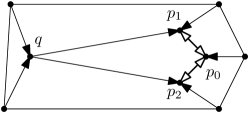
Figure 21: A subdivision, edges are oriented to endpoints where locked (not what we called a partial orientation, since some edges are doubly oriented). Removing the three edges incident to $p_{0}$ does not yield a subdivision, since a reflex angle occurs at $p_{1}$ and $p_{2}$. The edges incident to $\{p_{0},p_{1},p_{2}\}$ are not locked outside this set, but removing all incident edges creates a reflex angle at point $q$.

Definition 8.2 (prime, perfect coarsener; increment).

Let $S$ be a subdivision and let $U\subseteq\mathrm{\sf V^{\circ}}S$.

1. $U$ is called a coarsener, if (a) $U$ is incident to at least one edge in $S$, and (b) removal of the set $E_{U}$ of all edges incident to $U$ in $S$ yields a subdivision.

2. If $U$ is a coarsener, the increment of $U$, ${\sf inc}\hskip 1.00006ptU$, is defined as $|E_{U}|-2|U|$.

3. $U$ is called a prime coarsener, if (a) $U$ is a coarsener, (b) $U$ is a minimal coarsener, i.e., no proper subset of $U$ is a coarsener, and (c) all edges incident to $U$ are locked.

4. $U$ is called a perfect coarsener, if (a) $U$ is a prime coarsener, and (b) ${\sf inc}\hskip 1.00006ptU=1$.

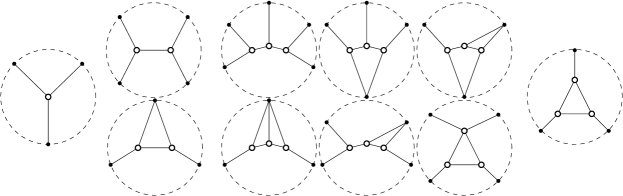
Figure 22: Prime coarseners, all perfect, except for the rightmost one (with ${\sf inc}=0$).

The following observation, a simple consequence of Obs. 7.3, explains the term “increment”.

Observation 8.3.

Let $S$ be a subdivision with coarsener $U$, and let $S^{\prime}$ be the subdivision obtained from $S$ by removing all edges incident to $U$. Then ${\sf sl}\hskip 1.00006ptS^{\prime}={\sf sl}\hskip 1.00006ptS+{\sf inc}\hskip 1.00006ptU$.

Observation 8.4.

1. Every subdivision $S$ with $\mathrm{\sf E^{\circ}}S\neq\emptyset$ has a coarsener (the set $\mathrm{\sf V^{\circ}}S$).

2. If $U_{1}$ and $U_{2}$ are coarseners, then $U_{1}\cap U_{2}$ is a coarsener, unless there is no edge of $S$ incident to $U_{1}\cap U_{2}$.

3. If $U_{1}$ and $U_{2}$ are prime coarseners, then $U_{1}=U_{2}$ or $U_{1}\cap U_{2}=\emptyset$.

4. If $U$ is a prime coarsener, then the subgraph of $S$ induced by $U$ is connected.

The following observation lists all ways of obtaining direct and perfect coarsenings.

Observation 8.5.

Let $S=(V,E)$ and $S^{\prime}$ be subdivisions.

1. $S^{\prime}$ is a direct coarsening of $S$ iff it is obtained from $S$ by one of the following.

   Adding a single point. For $p\in P\setminus V$, $S^{\prime}=(V\cup\{p\},E)$ (with ${\sf sl}\hskip 1.00006ptS^{\prime}={\sf sl}\hskip 1.00006ptS+1$).

   Removing a single unlocked edge. For $e\in E$, not locked by either of its two endpoints, $S^{\prime}=(V,E\setminus\{e\})$ (with ${\sf sl}\hskip 1.00006ptS^{\prime}={\sf sl}\hskip 1.00006ptS+1$).

   Isolating a prime coarsener. For $U$ a prime coarsener in $S$, $S^{\prime}$ is obtained from $S$ by removal of the set, $E_{U}$, of all edges incident to points in $U$, i.e., $S^{\prime}=(V,E\setminus E_{U})$ (with ${\sf sl}\hskip 1.00006ptS^{\prime}={\sf sl}\hskip 1.00006ptS+{\sf inc}\hskip 1.00006ptU$).

2. $S^{\prime}$ is a perfect coarsening of $S$ iff it is obtained from $S$ by adding a single point, removing a single unlocked edge, or by isolating a perfect coarsener.

We are prepared for the right formulation and proof of the Coarsening Lemma.

Lemma 8.6 (Coarsening Lemma for partial subdivisions).

Every subdivision of slack $D$ has at least $n-3-D$ perfect coarsenings (i.e., direct coarsenings of slack $D+1$).

Proof. We start with the case $D=0$, i.e., we have a triangulation $T$ and we want to show that there are at least $n-3$ direct coarsenings of slack $1$. Let $N:=|\mathrm{\sf V}T|$. We orient inner locked edges to their locking endpoints (recall that in a triangulation there is at most one such endpoint for each inner edge). Let $C_{i}$, $i\in\mathbb{N}_{0}$, be the number of points $p\in\mathrm{\sf V^{\circ}}T$ with indegree $i$. The number of unoriented, thus unlocked edges is at least $N-3-C_{3}$ (Lemma 4.9).

There are $n-N$ subdivisions obtained from $T$ by adding a single point, there are at least $N-3-C_{3}$ subdivisions obtained from $T$ by removing a single unlocked edge, and there are $C_{3}$ direct coarsenings obtained from $T$ by isolating an inner point of degree $3$. Adding up these numbers gives at least $n-3$ perfect coarsenings of $T$.

We let $S$ be a subdivision of slack $D\!\geq\!1$ assuming the assertion holds for slack less than $D$.

Case 1. There is a bystander $p_{0}\in\mathrm{\sf V^{\circ}}S$. Then $(\mathrm{\sf V}S\setminus\{p_{0}\},\mathrm{\sf E}S)$ is a subdivision of slack $D-1$ of $P\setminus\{p_{0}\}$ with at least $(n-1)-3-(D-1)=n-3-D$ perfect coarsenings of slack $D$. For each such perfect coarsening $S^{\prime}$, the subdivision $(\mathrm{\sf V}S^{\prime}\cup\{p_{0}\},\mathrm{\sf E}S^{\prime})$ is a direct coarsening of $S$ of slack $D+1$, thus a perfect coarsening.

Case 2. There is no bystander in $S$. Again we employ a partial orientation of $S$. The choice of the orientation is somewhat more intricate and we will proceed in three phases (Fig. 23). We keep the invariant that the unoriented inner edges are exactly the unlocked inner edges.

In a first phase, we orient all locked inner edges to all of their locking endpoints, i.e., we temporarily allow edges to be directed to both ends (to be corrected in the third phase); edges directed to both endpoints are called mutual edges. We can give the following interpretation to an edge directed from $p$ to $q$: If we decide to isolate $p$ (i.e., remove all incident edges of $p$) for a coarsening of $S$, then $q$ becomes a reflex point of some region and we have to isolate $q$ as well (i.e., every coarsener containing $p$ must contain $q$ as well). In particular, if $\{p,q\}$ is a mutual edge, then either both or none of the points $p$ and $q$ will be isolated. In fact, if we consider the graph $G$ with $\mathrm{\sf V}G:=\mathrm{\sf V^{\circ}}S$ and $\mathrm{\sf E}G$ the mutual edges in the current orientation, then in any coarsening of $S$ either all points in a connected component of $G$ are isolated, or none.

A connected component $K$ of $G$ is called a candidate component, (a) if all edges connecting $K$ with points outside are directed towards $K$, (b) no point in $K$ is incident to an unoriented edge, (c) all points in $K$ have indegree $3$, and (d) the mutual edges in $K$ do not form any cycle (i.e., they have to form a spanning tree of $K$). It follows that if $K$ has $k$ points then the number of edges is $3k-(k-1)=2k+1$. The term “candidate” refers to the fact that removing all edges incident to $K$ seems like a direct coarsening step with incrementing the slack by $1$ (Obs. 7.3); however, while individual edges connecting $K$ to the rest of the graph are not locked at their endpoints outside $K$, some of these edges collectively may actually create a reflex vertex in this way (see $K$ and $q$ in Fig. 23 (left)). So $K$ is only a candidate for a perfect coarsener.

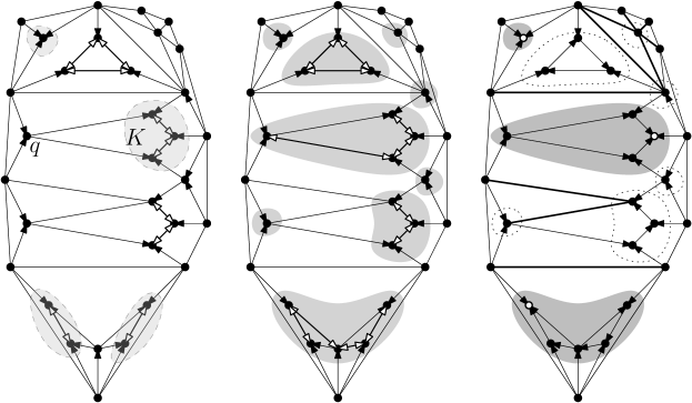
Figure 23: Orientation after phase 1, with candidate components shaded (left); after phase 2 (middle), with the connected components of $G^{*}$; after phase 3 (right), with unoriented edges bold (each of these can be removed for a coarsening of slack $1$ larger), and with the candidate components with a leader shaded (perfect coarseners).

We start the second phase of orienting edges further. In the spirit of our remarks about candidate components of $G$, suppose $q$ is an inner point outside a candidate $K$ of $G$ (thus all edges connecting $q$ to $K$ are directed from $q$ to $K$), such that removing the edges connecting $q$ to $K$ creates a reflex angle at $q$. Then we orient one (and only one) of the edges connecting $q$ to $K$, say $\{p,q\}$, also to $q$ (thereby making this edge mutual). We call all the edges connecting $K$ to $q$, except for $\{p,q\}$, the witnesses of the extra new orientation of $\{p,q\}$ from $p$ to $q$. We successively proceed orienting edges, with the graph $G$ of mutual edges evolving in this way (and candidate components growing or disappearing). The process will clearly stop at some point when the second phase is completed. We freeze $G$ and denote it by $G^{*}$.

Before we start the third phase, let us make a few crucial observations:

1. If $p,q$ are inner points in the same connected component of $G^{*}$, then any coarsener contains both or none (i.e., if a connected component is a coarsener, then it is prime). This holds after phase 1, and whenever we expand a connected component, it is maintained.

2. During the second phase, an edge can be witness only once, and it is and will never be directed to the endpoint where it witnesses. Why? (a) Before it becomes a witness, it connects different connected components of $G$, after that it is and stays in a connected component of $G$. (b) Before it becomes a witness, it is not directed to the endpoint to which it witnesses an orientation, after that it is and stays in a connected component of $G$ and can therefore not get an extra direction. (An unoriented edge can never get an orientation and it can never be a witness.)

3. If we remove, conceptually, for each incoming edge of a point $q$ the witnesses (which direct away from $q$) for the orientation of this edge to $q$, then among remaining incident edges, all the incoming edges are locked at $q$ (an incoming edge that was oriented already in the first phase to $q$ has no witness). In particular, the indegree of $q$ cannot exceed $3$, and if $q$ is incident to some not ingoing edge which is not a witness for any edge incoming at $q$, then the indegree of $q$ is at most $2$. (We might generate incoming edges to a point $q$ that are not consecutive around $q$.)

4. If an unoriented edge $e$ connects two points of the same connected component of $G^{*}$, then both endpoints have indegree at most $2$ (recall that this edge $e$ cannot be a witness at its endpoints). If an edge $e$ is directed from a connected component $K$ of $G^{*}$ to a point outside $K$, then the tail of this edge $e$ has indegree at most $2$ (recall that $e$ cannot be a witness at all, since its endpoints are in different connected components if $G^{*}$).

5. A candidate component $K$ of $G^{*}$ is a perfect coarsener. It is a coarsener (otherwise, we would have expanded it further), it is a prime coarsener (see (i) above) and ${\sf inc}\hskip 1.00006ptK=1$ (we have argued before that a candidate component increases the slack by exactly $1$).

The third phase will make sure that each mutual edge loses exactly one direction. Our goal is to have in every connected component $K$ of $G^{*}$ at most one point with indegree $3$. To be more precise, only candidate components have exactly one point with indegree $3$, others don’t. Consider a connected component $K$.

1. If the mutual edges form cycles in $K$, choose such a cycle $c$ and keep for each edge on $c$ one orientation so that we have a directed cycle, counterclockwise, say. All other mutual edges in $K$ keep the direction in decreasing distance in $G^{*}$ to $c$, ties broken arbitrarily. This completed, no point in $K$ has indegree $3$, since there is always a mutual edge incident that decreases the distance to $c$ and the incoming direction of this edge will be removed.

2. If $K$ has points of indegree at most $2$, choose one such point $p$ with indegree at most $2$, orient all mutual edges in $K$ in decreasing distance in $G^{*}$ to $p$, ties broken arbitrarily. Again, this completed, no point in $K$ will have indegree $3$.

3. If none of the above applies, the mutual edges of $K$ form a spanning tree and all points in $K$ have indegree $3$. Moreover, all edges connecting $K$ with points outside are directed towards $K$ and no edge within $K$ is unoriented (violation of these properties force a point of indegree at most $2$). So this is a candidate component. We choose an arbitrary point $p$ in $K$, call it the leader of $K$, and for all mutual edges keep the orientation of decreasing distance in $G^{*}$ to $p$ (ties cannot occur, mutual edges form a tree). Now the leader $p$ is the only point of $K$ with indegree $3$, all other points in $K$ have indegree exactly $2$.

Phase 3 is completed. Let us denote the obtained partial orientation of $S$ as ${\vec{S}}^{*}$. It has identified certain connected components of $G^{*}$ which have a leader of indegree $3$. In fact, every point of indegree $3$ after phase 3 is part of a perfect coarsener (probably of size $1$).

We can now describe a sufficient supply of perfect coarsenings of $S$. Let $N:=|\mathrm{\sf V}S|$ and let $C_{3}$ be the number of points of indegree $3$ in ${\vec{S}}^{*}$. We know that there are at least $N-3-D-C_{3}$ unoriented inner edges (Lemma 4.9).

1. There are $n-N$ perfect coarsenings obtained by adding a single point $p\in P\setminus\mathrm{\sf V}S$.

2. There are at least $N-3-D-C_{3}$ perfect coarsenings obtained by removing a single unoriented inner edge in ${\vec{S}}^{*}$.

3. And there are $C_{3}$ perfect coarsenings obtained by isolating all points in a candidate component in $G^{*}$ (with a leader of indegree $3$).

In this way we have identified at least $n-3-D$ perfect coarsenings.

Here are two immediate implications which we will need later: The first in the vertex-connectivity proof in Sec. 9 and the second for the result about covering of the bistellar flip graph by $(n-3)$-polytopes in Sec. 11.

Corollary 8.7.

Let $T\in{\cal T}_{\mathsf{part}}(P)$.

1. $T$ has at least $n-3$ flippable elements.

2. For every $x$ flippable in $T$ there are at least $n-4$ elements compatible with $x$.

Part (i) of the corollary was proved, without general position assumption, in [12, Thm. 2.1].

Corollary 8.8.

For every subdivision $S^{\prime}$ with ${\sf sl}\hskip 1.00006ptS^{\prime}\leq n-3$ there is a subdivision $S$ with $S^{\prime}\prec^{*}_{1}S$ and ${\sf sl}\hskip 1.00006ptS=n-3$.

9 $(n-3)$-Connectivity for Partial Triangulations

To complete the proof of Thm. 1.9, the $(n-3)$-vertex connectivity of the bistellar flip graph, we need again links, now for partial triangulations, which are graphs that represent the compatibility relation among flippable elements (Def. 7.10).

9.1 Link of a partial triangulation

Recall that if $x$ is a flippable element in a triangulation $T$ then $T_{\pm x}$ denotes the subdivision with ${\cal T}_{\mathsf{part}}{\langle T_{\pm x}\rangle}=\{T,T[x]\}$, and if $y$ is compatible with $x$, denoted $x\diamond y$, then $T_{\pm x,y}$ denotes the unique coarsening of slack $2$ of $T$ with $\{T[x],T,T[y]\}\subseteq{\cal T}_{\mathsf{part}}{\langle T_{\pm x,y}\rangle}$ (Def. 7.10).

Definition 9.1 (link of partial triangulation).

For $T\in{\cal T}_{\mathsf{part}}(P)$, the link of $T$, denoted ${\mathsf{Lk}}_{\mathsf{part}}T$, is the edge-weighted graph with vertices $\mathrm{\sf F}T:=\{x\in\mathrm{\sf V^{\circ}}T\cup\mathrm{\sf E^{\circ}}T\mid x\mbox{~{}flippable~{}in~{}}T\}$ and edge set $\{\{x,y\}\in{\mathrm{\sf F}T\choose 2}\mid x\diamond y\}$. The weight of an edge $\{x,y\}$ is $|{\cal T}_{\mathsf{part}}{\langle T_{\pm x,y}\rangle}|-2$ (which is $2$ or $3$).

(See Sec. 1.7 for some intuition for this definition.) We will see that it is enough to prove $(n-4)$-vertex connectivity of all links. The following lemma implies, via Lemma 2.4, that the vertex connectivity of links is determined by the minimum vertex degree.

Lemma 9.2.

The complement of ${\mathsf{Lk}}_{\mathsf{part}}T$ has no cycle of length $4$, i.e., if $(x_{0},x_{1},x_{2},x_{3})$ are flippable elements in $T$, then there exists $i\in\{0,1,2,3\}$ such that $x_{i}\diamond x_{i+1\!\bmod\!4}$.

Proof. Recall that all $p\in P^{\circ}\setminus\mathrm{\sf V^{\circ}}T$ are flippable and compatible with every flippable element (Obs. 7.11(i)), so we can assume $\{x_{0},x_{1},x_{2},x_{3}\}\subseteq\mathrm{\sf V^{\circ}}T\cup\mathrm{\sf E^{\circ}}T$. Moreover, if $p,q\in\mathrm{\sf V^{\circ}}T$ are two distinct points flippable in $T$, then $p\diamond q$ (Obs. 7.11(ii)). Hence, we assume that no two consecutive elements in the cyclic sequence $(x_{0},x_{1},x_{2},x_{3})$ are points; w.l.o.g. let $x_{0}=e$ and $x_{2}=f$ be edges.

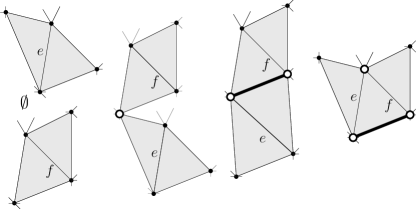
Figure 24: Intersections of boundaries of territories of two flippable edges.

Recall from Def. 3.2, that for an inner edge $e$ in a triangulation $T$, its territory ${\sf terr}\hskip 1.00006pte$, is defined as the interior of the closure of the union of the two regions in $T$ incident to $e$. Obviously, $e$ is flippable in $T$ iff the quadrilateral ${\sf terr}_{T}\hskip 1.00006pte$ is convex. Note that for an element $x$ to be incompatible with edge $e$, $x$ must appear on the boundary of ${\sf terr}\hskip 1.00006pte$, and analogously elements incompatible with $f$ must appear on the boundary of ${\sf terr}\hskip 1.00006ptf$.

We show that there is at most one flippable element in the intersection of the boundaries of ${\sf terr}\hskip 1.00006pte$ and ${\sf terr}\hskip 1.00006ptf$ (Fig. 24). This is obvious, if $\overline{{\sf terr}\hskip 1.00006pte}\cap\overline{{\sf terr}\hskip 1.00006ptf}$ is empty or a single point (recall that $\overline{A}$ denotes the closure of $A\subseteq\mathbb{R}^{2}$). If this intersection is an edge and its two endpoints, we observe that among any edge and its two incident points, at most one element can be flippable (inner degree $3$ points cannot be adjacent and cannot be incident to a flippable edge). This covers already all possibilties if ${\sf terr}\hskip 1.00006pte$ and ${\sf terr}\hskip 1.00006ptf$ are disjoint (since they are convex). Finally, $\overline{{\sf terr}\hskip 1.00006pte}\cap\overline{{\sf terr}\hskip 1.00006ptf}$ can be a triangle (see argument in the proof of Lemma 5.2), in which case the common boundary consists of the common endpoint of $e$ and $f$, clearly not flippable, and an edge with its two endpoints; again, at most one of these three can be flippable.

Lemma 9.3.

Given a triangulation $T$ with $x$ and $y$ flippable elements, $x\neq y$, every $x$-$y$-path of weight $w$ in ${\mathsf{Lk}}_{\mathsf{part}}T$ induces a $T$-avoiding $T[x]$-$T[y]$-path of length $w$ in the bistellar flip graph. Interior vertex-disjoint $x$-$y$-paths in the link induce vertex-disjoint $T[x]$-$T[y]$-paths.

Figure 25: From a path in the link to a path in the bistellar flip graph.

Proof. Given an $x$-$y$-path, we replace every edge $\{z^{\prime},z^{\prime\prime}\}$ on this path by $(T[z^{\prime}],\ldots,T[z^{\prime\prime}])$ (of length $2$ or $3$) which draws its ($1$ or $2$) internal vertices from ${\cal T}_{\mathsf{part}}{\langle T_{\pm z^{\prime},z^{\prime\prime}}\rangle}\setminus\{T[z^{\prime}],T,T[z^{\prime\prime}]\}$ (Fig. 25); these vertices must have distance $2$ from $T$ in the flip graph, while $T[z^{\prime}]$ and $T[z^{\prime\prime}]$ have distance $1$. In the resulting $T[x]$-$T[y]$-path, all internal vertices adjacent to $T$ (i.e., of the form $T[z]$) are distinct from internal vertices at other paths by assumption on the initial paths in the link. For vertices at distance $2$, suppose $T_{1}\in{\cal T}_{\mathsf{part}}{\langle T_{\pm z_{1}^{\prime},z_{1}^{\prime\prime}}\rangle}$ coincides with $T_{2}\in{\cal T}_{\mathsf{part}}{\langle T_{\pm z_{2}^{\prime},z_{2}^{\prime\prime}}\rangle}$, both at distance $2$ from $T$. Since ${\sf sl}\hskip 1.00006ptT_{\pm z_{1}^{\prime},z_{1}^{\prime\prime}}={\sf sl}\hskip 1.00006ptT_{\pm z_{2}^{\prime},z_{2}^{\prime\prime}}=2$, we have that ${\cal T}_{\mathsf{part}}{\langle T_{\pm z_{1}^{\prime},z_{1}^{\prime\prime}}\rangle}\cap{\cal T}_{\mathsf{part}}{\langle T_{\pm z_{2}^{\prime},z_{2}^{\prime\prime}}\rangle}$ either (a) equals $\{T\}$, (b) equals $\{T,T[z]\}$ for some $z$, or (c) $T_{\pm z_{1}^{\prime},z_{1}^{\prime\prime}}=T_{\pm z_{2}^{\prime},z_{2}^{\prime\prime}}$ (Lemma 7.9). In (a-b) $T_{\pm z_{1}^{\prime},z_{1}^{\prime\prime}}$ and $T_{\pm z_{2}^{\prime},z_{2}^{\prime\prime}}$ cannot possibly share a vertex at distance $2$ from $T$. Thus (c) holds. $T_{\pm z_{1}^{\prime},z_{1}^{\prime\prime}}=T_{\pm z_{2}^{\prime},z_{2}^{\prime\prime}}$ implies $\{z_{1}^{\prime},z_{1}^{\prime\prime}\}=\{z_{2}^{\prime},z_{2}^{\prime\prime}\}$.

Lemma 9.4.

For $T\in{\cal T}_{\mathsf{part}}(P)$, the link ${\mathsf{Lk}}_{\mathsf{part}}T$ is $(n-4)$-vertex connected.

Proof. Let $x$ be a vertex of ${\mathsf{Lk}}_{\mathsf{part}}T$. $T_{\pm x}$, a subdivision of slack $1$, has at least $n-4$ perfect coarsenings of slack $2$ (Lemma 8.6). Each such coarsening equals $T_{\pm x,y}$ for some $y\diamond x$, i.e., $y$ is a neighbor of $x$ in ${\mathsf{Lk}}_{\mathsf{part}}T$. Distinct coarsenings yield distinct compatible elements $y$ (since $\{T[x],T,T[y]\}\subseteq{\cal T}_{\mathsf{part}}{\langle T_{\pm x,y}\rangle}$ and ${\cal T}_{\mathsf{part}}{\langle T_{\pm x,y}\rangle}$ spans a cycle, $T[y]$ is determined as the other neighbor of $T$ on this cycle). That is, the minimum vertex degree in ${\mathsf{Lk}}_{\mathsf{full}}T$ is at least $n-4$. ${\mathsf{Lk}}_{\mathsf{part}}T$ has no cycle of length $4$ in its complement (Lemma 9.2). The lemma follows by Lemma 2.4.

9.2 Proof of Thm. 1.9

Proof. We know that the bistellar flip graph is connected, [11, Sec. 3.4.1], and it has at least $n-2$ vertices, since it is nonempty and every vertex has degree at least $n-3$ (Cor. 8.7(i)). Hence, for $(n-3)$-vertex connectivity, by the Local Menger Lemma 2.3 it is left to show that for any $T\in{\cal T}_{\mathsf{part}}(P)$ and flippable elements $x$ and $y$, there are at least $n-3$ vertex-disjoint $T[x]$-$T[y]$-paths in the bistellar flip graph. Since ${\mathsf{Lk}}_{\mathsf{part}}T$ is $(n-4)$-vertex connected (Lemma 9.4), ${\mathsf{Lk}}_{\mathsf{part}}T$ has at least $n-4$ vertex-disjoint $x$-$y$-paths (Menger’s Theorem 2.2). Therefore, there are at least $n-4$ vertex-disjoint $T[x]$-$T[y]$-paths disjoint from $T$ (Lemma 9.3). Together with the path $(T[x],T,T[y])$, the claim is established.

10 Regular Subdivisions by Successive Perfect Refinements

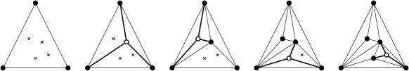
Figure 26: Stacked triangulations (which are always regular).

Suppose $h=3$ and consider stacked triangulations of $P$, i.e., we start with the triangulation $({\sf xtr}P,{\sf E_{\mathsf{hull}}})$, and then we successively add points in $P^{\circ}$ by connecting a new point to the three vertices of the triangle where it lands in (Fig. 26). It is easily seen that this yields regular triangulations. The result of this section is the following sufficient condition for the regularity of a subdivision (Def. 10.2 below), which can be seen as a generalization of the regularity of stacked triangulations (Fig. 27). The condition is not necessary, see Sec. 10.2.

Theorem 10.1.

If $S\prec^{*}_{1}\mathsf{S}_{\mathsf{triv}}$ for a subdivision $S$, then $S$ is a regular subdivision.

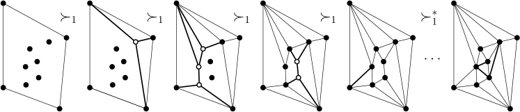
Figure 27: Successive perfect refinements of a trivial subdivison (all subdivisions regular).

In other words, all subdivisions, in particular, all triangulations in the $\prec_{1}$-lower closure of $\mathsf{S}_{\mathsf{triv}}$ are regular. This condition will eventually allow us to show the covering of the bistellar flip graph by graphs of $(n-3)$-polytopes. The proof of Thm. 10.1 stretches out over several definitions and lemmas with a conclusion in Sec. 10.6. Before we give a brief outline of this proof shortly in Sec. 10.3, we first introduce some notions.

10.1 Height functions, liftings, and regular subdivisions

Definition 10.2 (linear, compliant, realizing height function; regular subdivision).

A height function on $A\subseteq\mathbb{R}^{2}$ is a vector $\omega\in\mathbb{R}^{A}$, $p\mapsto\omega_{p}$. For $p=(x_{p},y_{p})\in A$, we let $p^{(\omega)}:=(x_{p},y_{p},\omega_{p})$, and for $B\subseteq A$, we set $B^{(\omega)}:=\{p^{(\omega)}\mid p\in B\}$. We say that $\omega$ is linear on $B\subseteq A$, if there exist $a$, $b$, and $c$ in $\mathbb{R}$ such that $\omega_{p}=ax_{p}+by_{p}+c$ for all $p\in B$, i.e., if $B^{(\omega)}$ is coplanar.

Let $S$ be a subdivision.

1. A height function $\omega$ on $\mathrm{\sf V}S$ is linear on $S$ if it is linear on $\mathrm{\sf V}S$. $\Lambda(S)$ denotes the set of linear height functions on $S$ and for $A\subseteq\mathrm{\sf V}S$, $\Lambda_{A}(S)$ denotes the set of height functions on $S$ linear on $A$.

2. A height function $\omega$ on $\mathrm{\sf V}S$ complies with $S$, (or is $S$-compliant), if for every region $r$ of $S$, $\omega$ is linear on $\mathrm{\sf V}r$ (including bystanders). Let $\Gamma(S)$ be the set of $S$-compliant height functions.

3. A height function $\omega$ on $\mathrm{\sf V}S$ realizes $S$, if $S$ is the projection of the lower convex hull of $\mathrm{\sf V}S^{(\omega)}$, with all points of $\mathrm{\sf V}S$ (also the bystanders) appearing on this lower convex hull.

4. $S$ is called regular if there is a height function realizing $S$.

Compliant height functions constitute a relaxation of realizing height functions (and of linear height functions): Every realizing height function (and every linear height function) is compliant. All height functions on a triangulation $T$ are compliant, i.e., $\Gamma(T)=\mathbb{R}^{\mathrm{\sf V}T}$. For the trivial subdivision $\mathsf{S}_{\mathsf{triv}}$, the compliant height functions are exactly the linear height functions, i.e., $\Gamma(\mathsf{S}_{\mathsf{triv}})=\Lambda(\mathsf{S}_{\mathsf{triv}})$. While compliant height functions exist for all triangulations and the trivial subdivision, this is a non-trivial property for general subdivisions.

Lemma 10.3.

Let $S$ be a subdivision.

1. $\Lambda(S)$ is a linear subspace of $\mathbb{R}^{\mathrm{\sf V}S}$ of dimension $\dim\Lambda(S)=3$. More generally, for every $B\subseteq\mathrm{\sf V}S$ with $|B|\geq 3$, $\Lambda_{B}(S)$ is a linear subspace of $\mathbb{R}^{\mathrm{\sf V}S}$ of dimension $|\mathrm{\sf V}S|-(|B|-3)$.

2. $\Gamma(S)=\bigcap_{r\in\mathrm{\sf R}S}\Lambda_{\mathrm{\sf V}r}(S)$ ($\mathrm{\sf R}S$ the set of regions of $S$).

3. $\Gamma(S)$ is a linear subspace of $\mathbb{R}^{\mathrm{\sf V}S}$ with $\Gamma(S)\supseteq\Lambda(S)$ and $\dim\Gamma(S)\geq|\mathrm{\sf V}S|-{\sf sl}\hskip 1.00006ptS$.

Proof. (i) is obvious and (ii) holds directly by definition.

Now, with ${\sf sl}\hskip 1.00006ptr=|\mathrm{\sf V}r|-3$ and ${\sf sl}\hskip 1.00006ptS=\sum_{r\in\mathrm{\sf R}S}(|\mathrm{\sf V}r|-3)$, assertion (iii) is an immediate consequence of (i), (ii), and the fact that intersecting linear subspaces of co-dimension $d_{1}$ and $d_{2}$ yields a subspace of co-dimension at most $d_{1}+d_{2}$:

$$|\mathrm{\sf V}S|-\dim\Gamma(S)\stackrel{{\scriptstyle\mbox{\footnotesize{\ref{it:iiLinCompliant}}}}}{{\leq}}\sum_{{r\in\mathrm{\sf R}S}}\left(|\mathrm{\sf V}S|-\dim\Lambda_{\mathrm{\sf V}r}(S)\right)\stackrel{{\scriptstyle\mbox{\footnotesize{\ref{it:iLinCompliant}}}}}{{=}}\sum_{{r\in\mathrm{\sf R}S}}\left(|\mathrm{\sf V}r|-3\right)={\sf sl}\hskip 1.00006ptS$$

We see that if ${\sf sl}\hskip 1.00006ptS<|\mathrm{\sf V}S|-3$, there are always compliant height functions not in $\Lambda(S)$. In order to extract among those a realizing height function we consider mountains and valleys in the lifting given by a compliant height function.

Definition 10.4 ($\omega$-lifting; $\omega$-labeling).

Let $\omega\in\Gamma(S)$. The $\omega$-lifting of $S$ is the unique piecewise linear function $f$ on the convex hull of $\mathrm{\sf V}S$, that is linear on every region $r$ of $S$, and ${f\raisebox{-0.79651pt}{\large$|$}}\raisebox{-1.89444pt}{${}_{\mathrm{\sf V}S}$}=\omega$.

We call $e\in\mathrm{\sf E^{\circ}}S$ a mountain, a valley, or flat in the $\omega$-lifting, depending on whether the directional derivative of function $f$ decreases, increases, or remains constant, respectively, as one traverses the $f$-lifted edge from one side to the other (at a mountain, the function is locally strictly concave, at a valley it is locally strictly convex). The $\omega$-labeling of $S$ assigns $\oplus$, $\ominus$, and $0$ to each inner edge of $S$, depending on whether the lifted edge is a mountain, a valley, or flat, respectively.

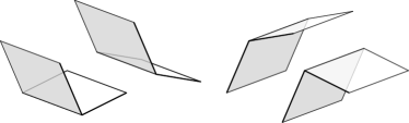
Figure 28: Valleys (left) and mountains (right).

Observation 10.5.

Let $\omega\in\Gamma(S)$.

1. $\omega$ is linear on $S$ iff the $\omega$-labeling of $S$ is constant $0$.

2. $\omega$ realizes $S$ iff the $\omega$-labeling of $S$ is constant $\ominus$.

10.2 Mother of examples

In order to understand the subtleties of whether a subdivision is regular or not, we should briefly discuss the mother of examples, see [11]. For this consider the configuration in Fig. 29. Whether or not the displayed subdivisions are regular or not depends on how exactly the three dashed lines (as indicated in $S$) meet.

1. If the three dashes lines meet in a common point, then $S$ is a regular subdivision, but none of $T^{\prime}$ and $T^{\prime\prime}$ is regular.

2. If the three dashes lines do not meet in a common point, then $S$ is not a regular subdivision, but one of $T^{\prime}$ and $T^{\prime\prime}$ is regular, the other one not.

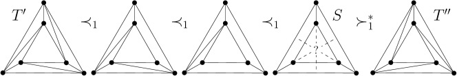
Figure 29: Exactly one of $S$, $T^{\prime}$, and $T^{\prime\prime}$ is regular. Which one depends on how the dashed lines meet.

The example allows us to clarify a few points.

1. The condition in Thm. 10.1 for regularity is not necessary (consider Case (b) with $T^{\prime}$ regular, and note $T^{\prime}\not\prec^{*}_{1}\mathsf{S}_{\mathsf{triv}}$). This is inherently so, since the condition in Thm. 10.1 depends only on the order type (or oriented matroid) of the point set. In fact, note that a perturbation of the point set does not change the order type of the set, but it affects how the dashed lines meet and, therefore, whether subdivisions are regular or not.

2. The condition in Thm. 10.1 cannot be generalized to: If $S\prec^{*}_{1}S^{\prime}$ and $S^{\prime}$ is regular, then $S$ is regular. In fact, adding a single edge in a subdivision may switch from regular to non-regular (Case (a)). The right generalization will be given in the Regularity Preservation Lemma 10.10 below.

10.3 Outline of proof of Thm. 10.1

It is easy to see that if $p$ is an inner point of degree $3$ in a triangulation $T$, then for any height function $\omega$ (which, as we observed, is $T$-compliant), the $\omega$-labeling assigns the same value to the three edges incident to $p$. We will generalize this observation for an $S$-compliant height function $\omega$ in two ways:

1. If $p\in\mathrm{\sf V^{\circ}}S$ and not all incident edges are $0$-labeled, then the $\oplus$-labeled and $\ominus$-labeled edges incident to $p$ cannot be separated by a line through $p$ (Lemma 10.7). (In particular, this forces the $\omega$-labeling to be constant on the edges incident to an inner point of degree $3$ in any subdivision.)

2. If $K$ is a perfect coarsener of $S$, then the $\omega$-labeling assigns the same label to all the edges $E_{K}$ incident to a perfect coarsener $K$ (Lemma 10.9).

Here is another simple observation about an inner point $p$ of degree $3$ in a triangulation $T$. Removing the three edges incident to $p$ (while keeping $p$ as a bystander) yields a subdivision $S$ with $T\prec_{1}S$. Obviously, if $S$ is a regular subdivision, then $T$ is a regular triangulation (this was behind our observation about stacked triangulations at the beginning of this section): Given a height function $\omega$ realizing $S$, we can always perturb $p$ downwards (decrease $\omega_{p}$ by a sufficiently small value $\varepsilon$), obtaining a height function that realizes $T$. Again, this allows an appropriate generalization:

1. Suppose $S$ is a regular subdivision with $\dim\Gamma(S)=|\mathrm{\sf V}S|-{\sf sl}\hskip 1.00006ptS$. Then every perfect refinement $S^{\prime}$ of $S$, i.e., $S^{\prime}\prec_{1}S$, is regular, and, moreover, $\dim\Gamma(S^{\prime})=|\mathrm{\sf V}S^{\prime}|-{\sf sl}\hskip 1.00006ptS^{\prime}$ (Regularity Preservation Lemma 10.10).

Since $\mathsf{S}_{\mathsf{triv}}$ is regular and $\dim\Gamma(\mathsf{S}_{\mathsf{triv}})=3=|\mathrm{\sf V}\mathsf{S}_{\mathsf{triv}}|-{\sf sl}\hskip 1.00006pt\mathsf{S}_{\mathsf{triv}}$, this immediately yields an inductive argument for Thm. 10.1. For the proof of (C), we consider the perfect coarsener $K$ of $S^{\prime}$ whose isolation leads to $S$, and a height function $\omega_{1}$ that realizes $S$. First, we show that $\dim\Gamma(S^{\prime})>\dim\Gamma(S)$, and, therefore, a height function $\omega^{\prime}\in\Gamma(S^{\prime})\setminus\Gamma(S)$ exists. According to (B), the $\omega^{\prime}$-labeling assigns the same label to all edges incident to $K$, and since $\omega^{\prime}\not\in\Gamma(S)$, this label cannot be $0$. Hence, either $\omega^{\prime}$ or $-\omega^{\prime}$ assigns constant $\ominus$, and it can be used for a controlled perturbation $\omega_{1}+\varepsilon\omega^{\prime}$ which realizes $S^{\prime}$.

We will now carefully work out these steps.

10.4 Valid $\{\oplus,\ominus,0\}$-edge labelings

Definition 10.6.

Let $S$ be a subdivision. Given a labeling $\alpha:\mathrm{\sf E^{\circ}}S\rightarrow\{\oplus,\ominus,0\}$, we call an inner point $p\in\mathrm{\sf V^{\circ}}S$ $\alpha$-pointed, if $\alpha$ is not constant $0$ on the edges incident to $p$, and if there is a line through $p$ that has all $\oplus$-labeled edges incident to $p$ strictly on one side and all $\ominus$-labeled edges incident to $p$ strictly on the other side of this line. (We do not require that both $\oplus$- and $\ominus$-labeled edges incident to $p$ exist.)

We call $\alpha$ a valid labeling of $\mathrm{\sf E^{\circ}}S$ if no point in $\mathrm{\sf V^{\circ}}S$ is $\alpha$-pointed (Fig. 30).

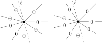
Figure 30: Patterns prohibited in valid labelings.

For example, for an inner point of degree $3$ in a subdivision, a valid labeling must assign the same label to its three incident edges. We can now prove (A) above.

Lemma 10.7.

Let $\omega$ be a height function compliant with subdivision $S$. Then the $\omega$-labeling of $S$ is a valid labeling of $\mathrm{\sf E^{\circ}}S$.

Proof. Let $p\in\mathrm{\sf V^{\circ}}S$ and suppose there is a line $\ell$ through $p$ that has all $\oplus$-labeled edges incident to $p$ on one side, and all $\ominus$-labeled edges incident to $p$ on the other side. Sweep a vertical plane $h$ parallel to $\ell$ in $\mathbb{R}^{3}$ over $p$ and observe its intersection with the $\omega$-lifting $f$. On the side of the $\oplus$-labeled edges, this intersection must be a locally concave function, on the side of the $\ominus$-labeled edges a locally convex function. Consequently, it has to be locally linear at the point when $h$ contains $p$ and $\ell$. Now it follows that $f$ must be locally linear around $p$ and all edges incident to $p$ must be flat.

Lemma 10.8.

Let $K$ be a perfect coarsener in a subdivision $S$. In every valid $\{\oplus,\ominus,0\}$-labeling of $\mathrm{\sf E^{\circ}}S$, the edges $E_{K}$ incident to $K$ all get the same label.

Proof. We plan to prove the following.

Claim. With reference to the orientation process in the proof of Lemma 8.6, after the second phase, in any valid labeling, the edges incident to a candidate component of $G^{*}$ get the same label.

It is not obvious from the proof of Lemma 8.6 that every perfect coarsener is identified by the three phase process. In order to close this gap (from the claim to the assertion of the lemma), isolate $K$ in $S$ obtaining a subdivision $S^{\prime}$ with a region $r$ containing the points in $K$. Let $V_{r}$ be the vertices of this regions, i.e., $V_{r}=\mathrm{\sf V}r\setminus\mathrm{\sf V^{by}}S^{\prime}$. Now consider the subgraph $S_{r}$ of $S$ induced by $V_{r}\cup K$. $K$ is a perfect coarsener of $S_{r}$ whose isolation yields the trivial subdivision of $V_{r}\cup K$. It is the only coarsener of $S-r$ and ${\sf sl}\hskip 1.00006ptS_{r}=|\mathrm{\sf V}S_{r}|-4$. Therefore, the procedure in the proof of Lemma 8.6 must identify $K$ as a candidate component after the second phase.

We establish the claim by showing the following invariant in the process during the second phase:

1. For every candidate component $K$, the edges $E_{K}$ incident to $K$ obtain the same label in any valid labeling.

2. An edge gaining a new orientation in the second phase and its witnesses obtain the same label in any valid labeling.

At the end of the first phase, a point with indegree $3$ in $\vec{S}$ has actually degree $3$ in $S$, and therefore any valid labeling must give the same label to all incident edges. Since in a candidate component $K$, all points have indegree $3$ in $\vec{S}$ (i.e., at this point, have degree $3$ in $S$) and since a connected component is connected [sic!], it easily follows that all edges incident to a candidate component must have the same label in any valid labeling.

During the second phase, a newly oriented edge and its witnesses are part of the edges incident to a candidate component. Hence, given (a), invariant (b) is maintained after an orientation step of phase 2. We are left to show that (a) is preserved. Consider a point $p$ of a candidate component. It must have indegree $3$, all incident edges are either ingoing or witnesses for an ingoing edge (otherwise, indegree $3$ is impossible); we know that each bundle of an ingoing edge and its witnesses have the same label, and such a bundle can be separated from the other incident edges by a line through the given point $p$ (this is why the edge was oriented in phase 2). Hence, due to a simple consideration, any valid labeling must assign the same label to all incident edges. (The simple consideration: Suppose a single bundle is labeled $\oplus$, then this bundle can be separated from the other two bundles by a line, contradiction. Suppose exactly two bundles are labeled $\oplus$, then the remaining bundle can be separated from these two $\oplus$-labeled bundles by a line, which is a contradiction. Hence, if any incident edge is labeled $\oplus$, then all incident edges must be labeled $\oplus$. Similarly, for $\ominus$.) This completes the proof of the claim, and thus of the lemma.

Now, with Lemma 10.7 we immediately get property (B).

Lemma 10.9.

If $\omega$ is an $S$-compliant height function, then the $\omega$-labeling is constant on any set of edges incident to a perfect coarsener of $S$ .

10.5 The Regularity Preservation Lemma

Lemma 10.10 (Regularity Preservation).

Let $S_{1}$ be a regular subdivision with $\dim\Gamma(S_{1})=|\mathrm{\sf V}S_{1}|-{\sf sl}\hskip 1.00006ptS_{1}$. If $S_{0}\prec_{1}S_{1}$, then $S_{0}$ is regular and $\dim\Gamma(S_{0})=|\mathrm{\sf V}S_{0}|-{\sf sl}\hskip 1.00006ptS_{0}$.

Proof. Let $\omega_{1}\in\mathbb{R}^{\mathrm{\sf V}S_{1}}$ be a height function that realizes $S_{1}$.

Case 1. $S_{1}$ is obtained from $S_{0}$ by adding a single point $p\in P^{\circ}\setminus\mathrm{\sf V^{\circ}}S_{0}$. Then ${\omega_{1}\raisebox{-0.79651pt}{\large$|$}}\raisebox{-1.89444pt}{${}_{\mathrm{\sf V}S_{0}}$}$ realizes $S_{0}$ and $S_{0}$ is regular. We have $\Gamma(S_{0})=\{{\omega\raisebox{-0.79651pt}{\large$|$}}\raisebox{-1.89444pt}{${}_{\mathrm{\sf V}S_{0}}$}\,\mid\,\omega\in\Gamma(S_{1})\}$. For $\omega\in\Gamma(S_{1})$, the value of $\omega_{p}$ ($p$ the added point) is determined by ${\omega\raisebox{-0.79651pt}{\large$|$}}\raisebox{-1.89444pt}{${}_{\mathrm{\sf V}S_{0}}$}$, i.e., $\dim\Gamma(S_{1})=\dim\Gamma(S_{0})$. Therefore,

$$\dim\Gamma(S_{0})=|\mathrm{\sf V}S_{1}|-{\sf sl}\hskip 1.00006ptS_{1}=(|\mathrm{\sf V}S_{0}|+1)-({\sf sl}\hskip 1.00006ptS_{0}+1)=|\mathrm{\sf V}S_{0}|-{\sf sl}\hskip 1.00006ptS_{0}~{}.$$

Case 2. $S_{1}$ is obtained from $S_{0}$ by removing a single unlocked edge or by isolating a perfect coarsener in $S_{0}$. We have $\mathrm{\sf V}S_{1}=\mathrm{\sf V}S_{0}$. The set $E^{*}:=\mathrm{\sf E}S_{0}\setminus\mathrm{\sf E}S_{1}$ is either a single unlocked edge or the set $E_{K}$ of edges incident to a perfect coarsener $K$ in $S_{0}$. Let $r^{*}$ be the region in $S_{1}$ generated by the removal of the edges in $E^{*}$.

We have $\Gamma(S_{0})\supseteq\Gamma(S_{1})$ and (with Lemma 10.3(iii) and ${\sf sl}\hskip 1.00006ptS_{0}={\sf sl}\hskip 1.00006ptS_{1}-1$)

$$\dim\Gamma(S_{0})\geq|\mathrm{\sf V}S_{0}|-{\sf sl}\hskip 1.00006ptS_{0}=|\mathrm{\sf V}S_{1}|-{\sf sl}\hskip 1.00006ptS_{1}+1=\dim\Gamma(S_{1})+1~{}.$$

Therefore, there must exist $\omega^{\prime}\in\Gamma(S_{0})\setminus\Gamma(S_{1})$, a height function that is not flat on $r^{*}$ and there is an edge in $E^{*}$ that is not flat in the $\omega^{\prime}$-lifting of $S_{0}$. In that case, all edges in $E^{*}$ are mountains or all are valleys (trivially true if $|E^{*}|=1$, otherwise by Lemma 10.9). Let us suppose that the $\omega^{\prime}$-labeling is constant $\ominus$ on $E^{*}$ (if not switch to $-\omega^{\prime}$). Now, for any sufficiently small positive $\varepsilon\in\mathbb{R}$, the height function $\omega_{0}:=\omega_{1}+\varepsilon\omega^{\prime}$ is compliant with $S_{0}$ and all inner edges in $S_{0}$ are valleys in the $\omega_{0}$-lifting of $S_{0}$ ($\varepsilon$ has to be small enough such that all valleys in the $\omega_{1}$-lifting remain valleys in $\omega_{0}$; this is a familar operation, see [11, Lemma 2.3.16]). This establishes that $S_{0}$ is regular.

We are left to show that $\dim\Gamma(S_{0})=|\mathrm{\sf V}S_{0}|-{\sf sl}\hskip 1.00006ptS_{0}$, or, equivalently, $\dim\Gamma(S_{0})=\dim\Gamma(S_{1})+1$. This holds, if for any two $\omega^{\prime}$, $\omega^{\prime\prime}$ in $\Gamma(S_{0})\setminus\Gamma(S_{1})$ there exists $a\in\mathbb{R}$ and $\omega\in\Gamma(S_{1})$ such that $\omega^{\prime}=a\omega^{\prime\prime}+\omega$. Suppose that all edges in $E^{*}$ are valleys in $\omega^{\prime}$, and all edges in $E^{*}$ are mountains in $\omega^{\prime\prime}$ (switch signs, if necessary). Now consider $\omega_{t}:=(1-t)\omega^{\prime}+t\omega^{\prime\prime}$, $t\in[0,1]$. There must be a value $t$ in $(0,1)$ where some edge in $E^{*}$ is flat in the $\omega_{t}$-lifting, but then all edges have to be flat and $\omega_{t}\in\Gamma(S_{1})$ (Lemma 10.9). We have shown $\omega^{\prime}=-\frac{t}{1-t}\omega^{\prime\prime}+\frac{1}{1-t}\omega_{t}$ with $\omega_{t}\in\Gamma(S_{1})$.

10.6 Proof of Thm. 10.1

Proof. If $S\prec^{*}_{1}\mathsf{S}_{\mathsf{triv}}$ then there is a sequence

$$S=S_{0}\prec_{1}S_{1}\prec_{1}\cdots\prec_{1}S_{\ell}=\mathsf{S}_{\mathsf{triv}}~{}.$$

$\mathsf{S}_{\mathsf{triv}}$ is regular, ${\sf sl}\hskip 1.00006pt\mathsf{S}_{\mathsf{triv}}=n-3$ and $\Gamma(\mathsf{S}_{\mathsf{triv}})=\Lambda(\mathsf{S}_{\mathsf{triv}})$, of dimension $3=n-{\sf sl}\hskip 1.00006pt\mathsf{S}_{\mathsf{triv}}=|\mathrm{\sf V}{\mathsf{S}_{\mathsf{triv}}}|-{\sf sl}\hskip 1.00006pt\mathsf{S}_{\mathsf{triv}}$. Along Lemma 10.10 we have an inductive argument that $S_{0}=S$ is regular.

We immediately get that successive perfect refinements of a subdivision $S^{*}$ fill the regions of $S^{*}$ with locally regular subdivisions.

Definition 10.11 (restriction of subdivision).

Let $S\preceq S^{\prime}$ be subdivisions, and let $r\in\mathrm{\sf R}S^{\prime}$. Then the restriction of $S$ to $r$, ${S\raisebox{-0.79651pt}{\large$|$}}\raisebox{-1.89444pt}{${}_{r}$}$, is the subgraph of $S$ induced by $\mathrm{\sf V}S\cap\overline{r}$ ($\overline{r}$ the closure of $r$).

Corollary 10.12.

Let $S\prec^{*}_{1}S^{\prime}$. For $r\in\mathrm{\sf R}S^{\prime}$, we have ${S\raisebox{-0.79651pt}{\large$|$}}\raisebox{-1.89444pt}{${}_{r}$}\prec^{*}_{1}\mathsf{S}_{\mathsf{triv}}(\mathrm{\sf V}r)$ and ${S\raisebox{-0.79651pt}{\large$|$}}\raisebox{-1.89444pt}{${}_{r}$}$ is a regular subdivision of $\mathrm{\sf V}r$.

Let us conclude this section with the remark, that successive perfect coarsening starting from a subdivision is a non-deterministic process, that may – even for the same subdivision – lead to $\mathsf{S}_{\mathsf{triv}}$ or not (Fig. 31).

Figure 31: Successive perfect coarsenings may lead to the trivial subdivisons (and thus imply regularity) or to another subdivision of slack $n-3$.

11 Implications of Regularity Preservation

11.1 Covering the bistellar flip graph with polytopes

Theorem 11.1.

The edge set of the bistellar flip graph of $P$ can be covered by subgraphs isomorphic to 1-skeletons of $(n-3)$-polytopes (which are products of secondary polytopes).

Proof. Given an edge $\{T,T[x]\}$ of the bistellar flip graph, let $S$ be a subdivision with $T_{\pm x}\prec^{*}_{1}S$ and ${\sf sl}\hskip 1.00006ptS=n-3$ (Cor. 8.8). For every region $r$ of $S$, the subdivisions ${T\raisebox{-0.79651pt}{\large$|$}}\raisebox{-1.89444pt}{${}_{r}$}$, ${T[x]\raisebox{-0.79651pt}{\large$|$}}\raisebox{-1.89444pt}{${}_{r}$}$, and ${T_{\pm x}\raisebox{-0.79651pt}{\large$|$}}\raisebox{-1.89444pt}{${}_{r}$}$ are regular subdivisions of $\mathrm{\sf V}r$; this holds, since $T\prec_{1}T_{\pm x}$ and $T[x]\prec_{1}T_{\pm x}$ (Lemma 7.8), thus $T\prec^{*}_{1}S$ and $T[x]\prec^{*}_{1}S$.

Now consider the product of polytopes (see [39])

$$\prod_{r\in\mathrm{\sf R}S}\Sigma\mbox{-}\mathsf{poly}(\mathrm{\sf V}r)~{},$$

where $\Sigma\mbox{-}\mathsf{poly}(A)$ denotes the secondary polytope of $A\subseteq P$ [11], see also Sec. 1.4, Thm. 1.11. The dimension of this product is $\sum_{r}(|\mathrm{\sf V}r|-3)={\sf sl}\hskip 1.00006ptS=n-3$. Its faces correspond to the refinements $S^{\prime}$ of $S$ such that for each region $r$ of $S$, ${S^{\prime}\raisebox{-0.79651pt}{\large$|$}}\raisebox{-1.89444pt}{${}_{r}$}$ is regular, i.e., this includes $T$ and $T[x]$ (as vertices), and $T_{\pm x}$ (as edge) (Cor. 10.12). This completes the argument.

      

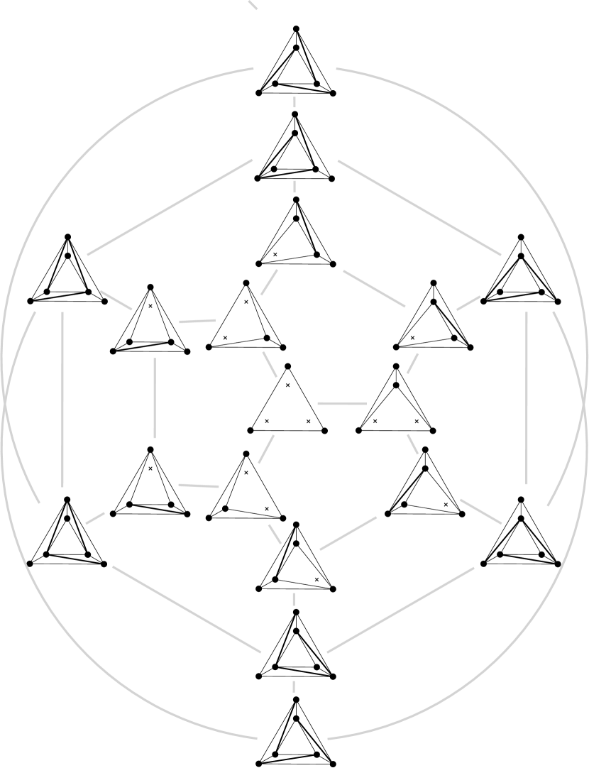
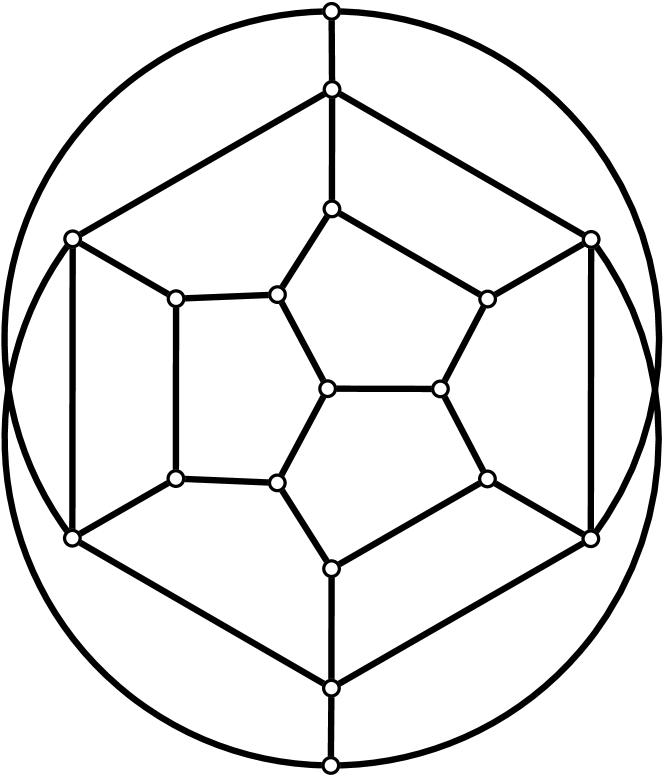
Figure 32: The bistellar flip graph of the mother-of-examples configuration.

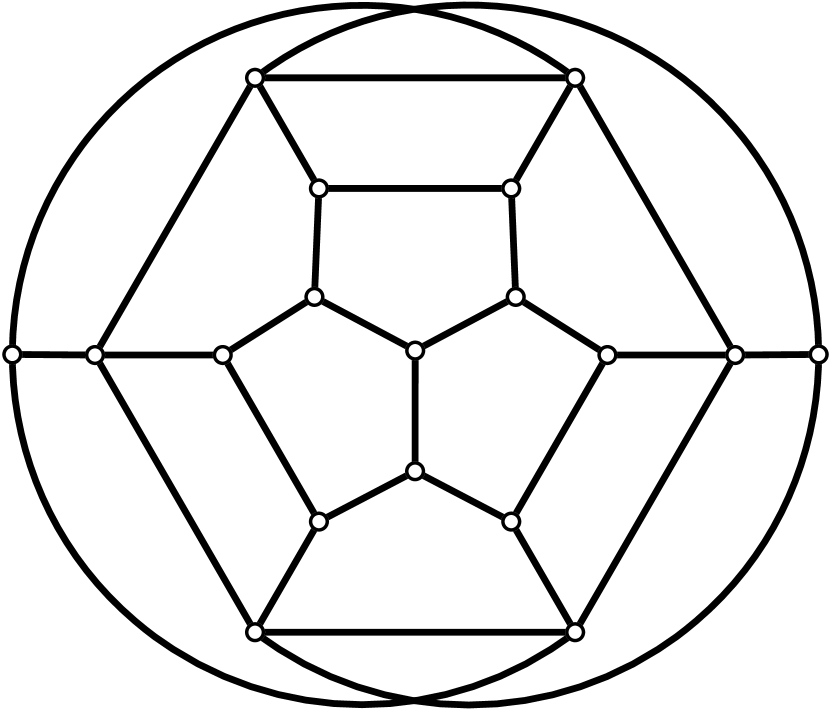
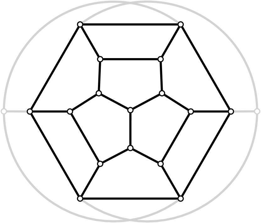
$=$ $\cup$

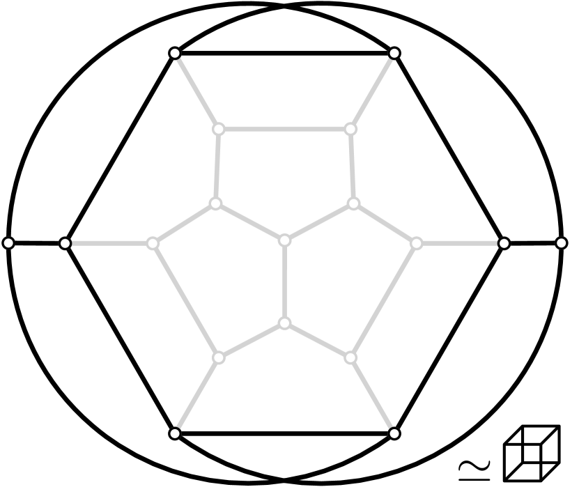
Figure 33: The bistellar flip graph of the mother-of-examples configuration as the union of the graphs of two $3$-polytopes.

11.2 Sets with all triangulations regular

We give characterizations of point sets for which all triangulations are regular (as, e.g., it is the case for point sets in convex position). In particular, we show that this can be easily read off the height of the partial order $\preceq$. In a first step we prove that property to be equivalent to requiring that all subdivisions are regular.

Lemma 11.2.

All subdivisions are regular iff all triangulations are regular.

Proof. The direction ($\Rightarrow$) is obvious.

For ($\Leftarrow$) it suffices to show that every non-regular subdivision $S$ with ${\sf sl}\hskip 1.00006ptS>0$ has a direct refinement which is not regular.

Case 1. $S$ has a bystander $p\in\mathrm{\sf V^{by}}S$. Clearly, the direct refinement $(\mathrm{\sf V}S\setminus\{p\},\mathrm{\sf E}S)$ is not regular iff $S$ is not regular.

Case 2. $S$ has no bystander. Since ${\sf sl}{S}>0$, $S$ must have an active region $r^{*}$ which is a $k$-gon for $k\geq 4$. Choose two crossing diagonals $e_{0}$ and $e_{1}$ in $r^{*}$ and consider the subdivisions $S_{i}:=(\mathrm{\sf V}S,\mathrm{\sf E}S\cup\{e_{i}\})$, $i=0,1$. We want to show that if $S$ is not regular, then at least one of $S_{0}$ and $S_{1}$ is not regular. So let us suppose that, for $i=0,1$, $\omega_{i}\in\mathbb{R}^{\mathrm{\sf V}S}$ is a height function realizing $S_{i}$ (as a regular subdivision) and, for $t\in[0,1]$, consider the convex combination $\omega_{t}:=(1-t)\omega_{0}+t\omega_{1}$.

We say that a height function $\omega$ respects region $r$ in subdivision $S$, if $\omega$ is linear on $\mathrm{\sf V}r$ and all points in $\mathrm{\sf V}S^{(\omega)}\setminus\mathrm{\sf V}r^{(\omega)}$ lie strictly above the plane spanned by $\mathrm{\sf V}r^{(\omega)}$. Clearly, $\omega$ realizes $S$ iff it respects all regions $r\in\mathrm{\sf R}S$. Moreover, if two height functions respect a region, then all convex combinations do.

It follows, that $\omega_{t}$ respects all regions in $\mathrm{\sf R}S$ except for $r^{*}$, since these are regions both in $S_{0}$ and $S_{1}$. We have that $e_{0}^{(\omega_{0})}$ lies below $e_{1}^{(\omega_{0})}$ (as segments in the lifting in $\mathbb{R}^{3}$), while $e_{1}^{(\omega_{1})}$ lies below $e_{0}^{(\omega_{1})}$ and, therefore, there must be a $t\in(0,1)$, where $e_{0}^{(\omega_{t})}$ and $e_{1}^{(\omega_{t})}$ intersect (in the lifting in $\mathbb{R}^{3}$). For that value of $t$, $\omega_{t}$ is linear on $\mathrm{\sf V}r^{*}$. Moreover, all edges in ${S\raisebox{-0.79651pt}{\large$|$}}\raisebox{-1.89444pt}{${}_{r}$}$ are valleys in the $\omega_{t}$-lifting, since these are valleys both in the $\omega_{0}$-lifting and the $\omega_{1}$-lifting (and that property is preserved for all convex combinations of $\omega_{0}$ and $\omega_{1}$). Hence, $\omega_{t}$ realizes $S$ and we have a contradiction.

We recall the definition of the height of an element in a partial order, and of the height of the partial order.

Definition 11.3 (height).

The height, $0ptS$, of a subdivision $S$ (in the partial order $\preceq$) is recursively defined: (a) If $S$ is a triangulation, then $0ptS:=0$, and (b) if $S$ is not a triangulation, then $0ptS:=1+\max_{S^{\prime}\prec_{\mathrm{dir}}S}0ptS^{\prime}$. (Equivalently, $0ptS$ is the size of the longest $\preceq$-chain ending in $S$ minus $1$.) We let $0pt_{\mathsf{max}}=0pt_{\mathsf{max}}(P)$ be the maximum height of any subdivision of $P$ (i.e., $0pt_{\mathsf{max}}=0pt\mathsf{S}_{\mathsf{triv}}$).

Theorem 11.4.

The following six conditions are equivalent.

1. All triangulations are regular.

2. All subdivisions are regular.

3. $0pt_{\mathsf{max}}=n-3$.

1. $\prec_{\mathrm{dir}}=\prec_{1}$.

2. $0pt={\sf sl}$.

Proof. For (i) $\Leftrightarrow$ (ii) see Lemma 11.2. For the rest we show the implication cycles

all subdivisions are regular $\stackrel{{\scriptstyle\mathrm{(a)}}}{{\Rightarrow}}$ $0pt_{\mathsf{max}}=n-3$ $\stackrel{{\scriptstyle\mathrm{(b)}}}{{\Rightarrow}}$ $\prec_{\mathrm{dir}}=\prec_{1}$ $\stackrel{{\scriptstyle\mathrm{(c)}}}{{\Rightarrow}}$ all subdivisions are regular

and

$0pt_{\mathsf{max}}=n-3$ $\stackrel{{\scriptstyle\mathrm{(b)}}}{{\Rightarrow}}$ $\prec_{\mathrm{dir}}=\prec_{1}$ $\stackrel{{\scriptstyle\mathrm{(d)}}}{{\Rightarrow}}$ $0pt={\sf sl}$ $\stackrel{{\scriptstyle\mathrm{(e)}}}{{\Rightarrow}}$ $0pt_{\mathsf{max}}=n-3$.

(a) All subdivisions are regular $\Rightarrow$ $0pt_{\mathsf{max}}=n-3$.   This is well known and discussed, e.g., in “Twelve proofs of non-regularity” in [11, Sec. 7.1.2, (6)]: On the one hand, if all subdivisions are regular, they all correspond to faces of the secondary polytope, an $(n-3)$-polytope where every chain of proper faces (excluding the empty face and the polytope itself) has size at most $(n-3)$. On the other hand, if $0pt_{\mathsf{max}}>n-3$, that gives a chain of size exceeding $n-3$ of non-trivial subdivisions.

(b) $0pt_{\mathsf{max}}=n-3$ $\Rightarrow$ $\prec_{\mathrm{dir}}=\prec_{1}$.   Consider a maximal chain $S_{0}\prec_{\mathrm{dir}}S_{1}\prec_{\mathrm{dir}}\cdots\prec_{\mathrm{dir}}S_{m}$; because of maximality, $S_{0}$ is a triangulation (of slack $0$), and $S_{m}=\mathsf{S}_{\mathsf{triv}}$ (of slack $n-3$). We know that ${\sf sl}\hskip 1.00006ptS_{i}\leq{\sf sl}\hskip 1.00006ptS_{i-1}+1$ (Lemma 11.5 below) with equality iff $S_{i-1}\prec_{1}S_{i}$. It follows that $m\geq n-3$. Moreover, if $m=n-3$ (which is given if $0pt_{\mathsf{max}}=n-3$), then $S_{i-1}\prec_{1}S_{i}$ for all $i=1,2,\ldots,n-3$. Since every pair $S^{\prime}\prec_{\mathrm{dir}}S$ is part of a maximal chain, the claim follows.

(c) $\prec_{\mathrm{dir}}=\prec_{1}$ $\Rightarrow$ all subdivisions are regular.   Every subdivision $S$ has a chain of direct coarsenings to $\mathsf{S}_{\mathsf{triv}}$. If every direct coarsening is a perfect coarsening, this shows $S\prec^{*}_{1}\mathsf{S}_{\mathsf{triv}}$ and therefore $S$ is regular (Thm. 10.1).

(d) $\prec_{\mathrm{dir}}=\prec_{1}$ $\Rightarrow$ $0pt={\sf sl}$.   For proving $0ptS={\sf sl}\hskip 1.00006ptS$, we can proceed by induction on the height of $S$, where the induction basis holds without assumptions. With the assumption of $\prec_{\mathrm{dir}}=\prec_{1}$ and with the induction hypothesis

$$0ptS=1+\max_{S^{\prime}\prec_{\mathrm{dir}}S}0ptS^{\prime}=1+\max_{S^{\prime}\prec_{1}S}0ptS^{\prime}=1+\max_{S^{\prime}\prec_{1}S}{\sf sl}\hskip 1.00006ptS^{\prime}=1+\max_{S^{\prime}\prec_{1}S}({\sf sl}\hskip 1.00006ptS-1)={\sf sl}\hskip 1.00006ptS$$

For the last equality, note that for a subdivision that is not a triangulation, a perfect refinement can always be obtained by simply adding an edge, or by involving a bystander as a point of degree $3$. If there is no edge to add and if there is no bystander, we have a triangulation.

(e) $0pt={\sf sl}{}$ $\Rightarrow$ $0pt_{\mathsf{max}}=n-3$.   If $0pt={\sf sl}{}$, then $0pt_{\mathsf{max}}=0pt\mathsf{S}_{\mathsf{triv}}={\sf sl}\hskip 1.00006pt\mathsf{S}_{\mathsf{triv}}=n-3$.

11.3 More properties of coarseners

We derive two more properties of prime and perfect coarseners, Lemma 11.5, which we used in the proof of Thm. 11.4 above, and Lemma 11.6, which we will need in Sec. 11.4 below.

Lemma 11.5.

${\sf inc}\hskip 1.00006ptU\leq 1$ for every prime coarsener $U$ in a subdivision $S$.

Proof. Let $r$ be the region in $S^{\prime}$ obtained by removing from $S$ the edges $E_{U}$ incident to $U$. The subgraph of $S$ induced by $U$ is connected (Obs. 8.4(iv)), that is, all points of $U$ have to lie in the same region of $S^{\prime}$. We consider the restriction ${S\raisebox{-0.79651pt}{\large$|$}}\raisebox{-1.89444pt}{${}_{r}$}$ (Def. 10.11), a subdivision of $\mathrm{\sf V}{S\raisebox{-0.79651pt}{\large$|$}}\raisebox{-1.89444pt}{${}_{r}$}=\mathrm{\sf V}S\,\cap\,\overline{r}$. Isolating $U$ in ${S\raisebox{-0.79651pt}{\large$|$}}\raisebox{-1.89444pt}{${}_{r}$}$ yields ${S^{\prime}\raisebox{-0.79651pt}{\large$|$}}\raisebox{-1.89444pt}{${}_{r}$}$, the trivial subdivision of $\mathrm{\sf V}{S\raisebox{-0.79651pt}{\large$|$}}\raisebox{-1.89444pt}{${}_{r}$}$. Therefore,

$${\sf sl}\hskip 1.00006pt{S\raisebox{-0.79651pt}{\large$|$}}\raisebox{-1.89444pt}{${}_{r}$}+{\sf inc}{U}\stackrel{{\scriptstyle\mbox{\footnotesize{Obs.}\,\ref{o:Increment}}}}{{=}}{\sf sl}\hskip 1.00006pt{S^{\prime}\raisebox{-0.79651pt}{\large$|$}}\raisebox{-1.89444pt}{${}_{r}$}=|\mathrm{\sf V}{S\raisebox{-0.79651pt}{\large$|$}}\raisebox{-1.89444pt}{${}_{r}$}|-3,$$

that is, ${\sf inc}{U}=|\mathrm{\sf V}{S\raisebox{-0.79651pt}{\large$|$}}\raisebox{-1.89444pt}{${}_{r}$}|-3-{\sf sl}\hskip 1.00006pt{S\raisebox{-0.79651pt}{\large$|$}}\raisebox{-1.89444pt}{${}_{r}$}$. On the one hand, $U$ is the only coarsener of ${S\raisebox{-0.79651pt}{\large$|$}}\raisebox{-1.89444pt}{${}_{r}$}$ (since $U$ is prime and it exhausts all inner points in $\mathrm{\sf V}{S\raisebox{-0.79651pt}{\large$|$}}\raisebox{-1.89444pt}{${}_{r}$}$). On the other hand, the Coarsening Lemma 8.6 guarantees $|\mathrm{\sf V}{S\raisebox{-0.79651pt}{\large$|$}}\raisebox{-1.89444pt}{${}_{r}$}|-3-{\sf sl}\hskip 1.00006pt{S\raisebox{-0.79651pt}{\large$|$}}\raisebox{-1.89444pt}{${}_{r}$}$, i.e., ${\sf inc}{U}$ (perfect) coarsenings of ${S\raisebox{-0.79651pt}{\large$|$}}\raisebox{-1.89444pt}{${}_{r}$}$. Therefore, ${\sf inc}{U}\leq 1$.

Lemma 11.6.

A prime coarsener $U$ inducing a tree in its subdivision $S$ is perfect.

Proof. Let $k:=|U|$ and let $\ell$ be the number of edges in $\mathrm{\sf E^{\circ}}S$ that are incident to exactly one point in $U$. We have $|E_{U}|=(k-1)+\ell$. Since every point in $U$ has degree at least $3$, we have $|E_{U}|\geq\frac{3k+\ell}{2}$. Hence, $(k-1)+\ell\geq\frac{3k+\ell}{2}$, i.e., $\ell\geq k+2$. Now ${\sf inc}{U}=|E_{U}|-2|U|=(k-1)+\ell-2k=\ell-k-1\geq 1$, i.e., by Lemma 11.5, ${\sf inc}{U}=1$.

11.4 Large minimal sets with non-regular triangulations – Proof of Thm. 1.14

Observation 11.7.

If $P^{\prime}\subseteq P$ and $P^{\prime}$ has non-regular triangulations, then $P$ has non-regular triangulations.

Given a set $P$ with non-regular triangulations, is there always a small subset $P^{\prime}$ of $P$ that witnesses this fact? This is a question asked by F. Santos [33]. An equivalent reformulation is: How large can minimal sets $P$ with non-regular triangulations be? (Here, “minimal” means that every proper subset of $P$ has only regular triangulations.) Santos [33] describes such a minimal set of $8$ points and conjectures this to be the largest example of such a minimal set. We will show that there exist such minimal sets of arbitrarily large (even) size.

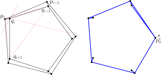
Figure 34: A twisted double-gon of $10$ points with subdivision $S^{\Box}$ (left). Subset $P^{*}$ (case $p_{0}^{*}=q_{0}$) of a twisted double-gon (right).

Definition 11.8 (twisted double-gon).

A set $P$ of $n$ points in general position, $n=2k$ even, is called a twisted double-gon if the following holds.

1. $|{\sf xtr}P|=k$.

Let $p_{0},p_{1},\ldots,p_{k-1}$ be a counter-clockwise numbering of ${\sf xtr}P$ along the boundary of the convex hull of $P$.

1. The set $Q:=P^{\circ}$ of inner points is in convex position.

There is a numbering $q_{0},q_{1},\ldots,q_{k-1}$ of $Q$ following the order along the boundary of the convex hull of $Q$ such that for all $i$, $0\leq i\leq k-1$, it holds:

1. $q_{i}$ is extreme in $P\setminus\{p_{i}\}$.

2. $q_{i}$ is extreme in $P\setminus\{p_{i-1},q_{i-1}\}$.

3. $q_{i}$ lies in the triangle $q_{i-1}p_{i}q_{i+1}$.

Fig. 34 indicates that such twisted double-gons exist for all even $n\geq 6$. For $n=6$, this is the mother-of-examples configuration (Sec. 10.2). Here are a few simple observations.

Observation 11.9.

Let $P$ be a twisted double-gon, with notation as in Def. 11.8.

1. The graph $S^{\Box}:=(P,{\sf E_{\mathsf{hull}}}\cup\{\{q_{i},p_{i}\},\{q_{i},q_{i+1\!\bmod\!k}\}\mid i=0,1,\ldots,k-1\}$ is a subdivision (uses (II) and (V)). Its slack is $n-3$.

2. If $q_{i}$ is involved in a subdivision of a subset of $P$ where it is not extreme, it is connected to $p_{i}$ (by (III)) and to at least one of $\{p_{i-1},q_{i-1}\}$ (by (IV)).

Here comes the lemma that shows that twisted double-gons constitute examples showing Thm. 1.14.

Lemma 11.10.

If $P$ is a twisted double-gon, then

1. $P$ has a non-regular triangulation, and

2. any proper subset of $P$ has only regular triangulations.

Proof. (i) Since ${\sf sl}\hskip 1.00006ptS^{\Box}=n-3$, we have $0ptS\geq n-3$ (by Lemma 11.5), therefore $0pt\mathsf{S}_{\mathsf{triv}}>n-3={\sf sl}\hskip 1.00006pt\mathsf{S}_{\mathsf{triv}}$ and $0pt\neq{\sf sl}$. Thm. 11.4 implies that $P$ has non-regular triangulations. Note that we do not claim that $S^{\Box}$ is a non-regular subdivision; this depends on the concrete coordinates of the point set $P$.

(ii) We remove $p_{0}$ or $q_{0}$ from $P$, we denote the resulting set by $P^{*}$ with $p_{0}^{*}$ the point among $p_{0}$ and $q_{0}$ remaining in $P^{*}$, see Fig. 34 (right). If we can show that all triangulations of $P^{*}$ are regular, then the proof is complete (by symmetry and Obs. 11.7).

It is enough to show that any prime coarsener $U$ of any subdivision $S$ of $P^{*}$ is perfect (by Lemma 11.5 this is equivalent to ${\sf inc}{U}=|E_{U}|-2|U|\geq 1$), since then $\prec_{\mathrm{dir}}=\prec_{1}$ and Thm. 11.4 can step in. So let us consider such a prime coarsener $U$, let $E^{\mathrm{in}}_{U}$ be the edges in $S$ connecting two points in $U$, and let $E^{\mathrm{out}}_{U}$ be the set of edges in $S$ connecting a point in $U$ to a point in $\mathrm{\sf V}S\setminus U$. We have $E_{U}=E^{\mathrm{in}}_{U}\cup E^{\mathrm{out}}_{U}$.

1. The subgraph of $S$ induced by $U$ has to be connected (since $U$ is prime, Obs. 8.4(iv)), hence $|E^{\mathrm{in}}_{U}|\geq|U|-1$.

2. If the subgraph of $S$ induced by $U$ is a tree, then, by Lemma 11.6, $U$ is a perfect coarsener.

So let us assume that $U$ does not span a tree, which implies $|E^{\mathrm{in}}_{U}|\geq|U|$.

1. Every point in $U$ has to connect to at least one point in $\mathrm{\sf V}S\setminus U$. This holds, since $U\subseteq Q\setminus\{q_{0}\}$ and $q_{i}\in U$, $i\geq 1$, has to connect to $p_{i}$ (Obs. 11.9(ii)). Hence, $|E^{\mathrm{out}}_{U}|\geq|U|$.

At this point we have already shown that $|E_{U}|=|E^{\mathrm{in}}_{U}|+|E^{\mathrm{out}}_{U}|\geq 2|U|$. Therefore, ${\sf inc}{U}\geq 0$, and $U$ is perfect unless $|E^{\mathrm{in}}_{U}|=|U|$ and $|E^{\mathrm{out}}_{U}|=|U|$.

1. Let $j:=\min\{i\in\mathbb{N}\mid i\geq 1,q_{i}\in U\}$. If $j=1$, i.e., $q_{1}\in U$, then $q_{1}$ connects to $p_{1}$ and $p_{0}^{*}$. Hence, $|E^{\mathrm{out}}_{U}|\geq|U|+1$. If $j\geq 2$, then $q_{j}$ has to connect to $p_{j}$ and $p_{j-1}$ (by (by Obs. 11.9(ii)), since $q_{j-1}$ is not available). Hence, $|E^{\mathrm{out}}_{U}|\geq|U|+1$.

We can conclude that $U$ has to be perfect.

12 Discussion and Open Problems

We conclude by briefly discussing some questions that naturally arise in connection with this work.

12.1 The min-degree bound for small sets

We have put some effort into getting rid of the “$P$ large enough”-condition in the min-degree bound of Thm. 1.7(i) for the edge flip graph. We have, however, not tried to find counter-examples by checking the Graz order type data base, [1]. Such an endeavour is not trivial, since an ad-hoc approach would have to produce and check vertex connectivity for reasonably large edge flip graphs, even when the underlying sets have no more than $11$ points.

12.2 General vs. special position

When abandoning the general position assumption, i.e., allowing collinearities of $3$ or more points can occur, the situation changes significantly. The edge flip graph may degenerate to a single vertex even for large point sets (Fig. 35).

         

Figure 35: Point sets with a unique full triangulation.

For bistellar flips, new flips as shown in Fig. 36 come into play. Thm. 1.8 ([12], see also [11, Thm. 3.4.9]) still holds in this situation and $n-3$ bistellar flips are guaranteed. We are currently investigating with N. Grellier to what extent our methods generalize from general to special position towards $(n-3)$-vertex connectivity of the bistellar flip graph, which is by no means obvious.

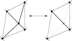
Figure 36: A flip in the presence of collinearities.

12.3 Stably regular triangulations

It might be interesting to understand, which regular triangulations are captured by Thm. 10.1, i.e., partial triangulations in the $\prec^{*}_{1}$-lower closure of $\mathsf{S}_{\mathsf{triv}}$. From the discussion in Sec. 10.2 (and Fig. 29) we recall one reason why this condition for regularity cannot possibly be necessary: It depends only on the order type (or oriented matroid) of $P$, while regularity depends on the coordinates of the point set. So let us define a partial triangulation $T$ of $P$ stably regular, if it is regular on any realization of the order type of $P$.  We believe that Thm. 10.1 goes as far as one can go with an order type based condition.

Conjecture 12.1.

A triangulation $T\in{\cal T}_{\mathsf{part}}(P)$ is stably regular iff $T\prec^{*}_{1}\mathsf{S}_{\mathsf{triv}}$.

One might ask whether the subdivisions in the $\prec^{*}_{1}$-down set of $\mathsf{S}_{\mathsf{triv}}$ correspond to the face lattice of a polytope. In general, this is not the case, it is not even an abstract polytope, (see [26, Chap. 2A] for abstract polytopes): We can choose ${\sf sl}\hskip 1.00006ptS$ as a rank function, have $\mathsf{S}_{\mathsf{triv}}$ as maximal/greatest element, and add an empty face as minimal/least element of rank $-1$. All flags (i.e., maximal chains) have the same size. But we fail on the so-called diamond axiom: “If $S$ is a subface of $S^{\prime}$ with the ranks differing by $2$, then there are exactly $2$ faces strictly between $S$ and $S^{\prime}$.” Fig. 31 shows an example where this axiom fails: $S$ and $\mathsf{S}_{\mathsf{triv}}$ in this figure differ by $2$ in slack, but there is only one subdivision strictly in between the two (in the $\prec_{1}$-order).

12.4 Minimal sets with non-regular triangulations

In Sec. 11.4 we have identified arbitrarily large minimal sets with non-regular triangulations. Given that such sets of arbitrary size exist, it is not clear how to check efficiently whether a set allows only regular triangulations. A first step would be to understand all minimal sets with non-regular triangulations. It is possible that twisted double-gons as defined in Def. 11.8 are the only such sets.

12.5 The fundamental group

Consider the set of closed walks in an edge or bistellar flip graph, starting in a fixed triangulation $T^{*}$. Consider a cycle $c=(T_{0},T_{1},\ldots,T_{k-1})$, $k\geq 2$, in the flip graph, i.e., $T_{i}$ and $T_{i+1\!\bmod\!k}$ are adjacent triangulations for $0\leq i<k$. An insertion of $c$ adds $c$ before an occurrence of $T_{0}$ in a closed walk, and a deletion of $c$ removes $c$ if it occurs before $T_{0}$ in a closed walk. Let us consider two closed walks equivalent, if they can be obtained from each other by insertion and deletion of cycles of length $2$, or of cycles spanned by the refinements of a subdivision of slack $2$ (these are $4$- or $5$-cycles). Lubiw et al. [25] show that in the edge flip graph all closed walks containing a triangulation $T^{*}$ are equivalent to the trivial walk $(T^{*})$; in other words, the fundamental group of the complex spanned by slack $2$ subdivisions (which correspond to the $2$-faces of the flip complex) is trivial. This is the decisive step in proving the orbit conjecture of [7] (see discussion in Sec. 1.5). It is natural to ask, whether the analogous result holds for the bistellar flip graph, or, more generally, whether there is a bistellar analogue of the flip complex.

12.6 Higher dimensions

Flip graphs can be defined on triangulations in higher dimensions, i.e., tetrahedralizations in $\mathbb{R}^{3}$, etc. , see [11], but even for sets of points in convex and general position in $3$-space it is open, whether these graphs are always connected. As mentioned before, because of the Local Menger Lemma 2.3, we were able to show high vertex connectivity without ever providing any evidence that the graph is connected. Basically, we showed high vertex connectivity of the connected components of the flip graphs, and Lawson gave us the connectedness on top of it. Still, it might be interesting to see whether one can show, e.g., $(n-4)$-vertex connectivity for bistellar flip graphs of sets in convex and general position in $\mathbb{R}^{3}$. A first step is supplied: There are always at least $n-4$ flips for such sets [11, Prop. 3.6.19].

12.7 Mixing rate of the random flip process

Last, but not least, a natural next question is to show expansion properties of the flip graphs, ideally yielding rapid mixing of the process of flipping random edges in the flip graph. This is known for points in convex positions, still with a big gap between the upper bound of $O(n^{5})$ and the lower bound of $\Omega(n^{3/2})$ (Mcshine & Tetali 1998, [27], and Molloy et al. 2001, [29]). There are related results for lattice point sets by Caputo et al. 2013, [8].

References

- [1] Aichholzer, O., Aurenhammer, F., and Krasser, H. Enumerating order types for small point sets with applications. Order 19, 3 (2002), 265–281.
- [2] Aichholzer, O., Hurtado, F., and Noy, M. A lower bound on the number of triangulations of planar point sets. Comput. Geom. Theory Appl. 29, 2 (Oct. 2004), 135–145.
- [3] Balinski, M. L. On the graph structure of convex polyhedra in -space. Pacific J. Math. 11, 2 (1961), 431–434.
- [4] Bern, M. W., Shewchuk, J. R., and Amenta, N. Triangulations and mesh generation. In Handbook of Discrete and Computational Geometry, Third Edition, C. D. Toth, J. O’Rourke, and J. E. Goodman, Eds. Chapman and Hall/CRC, 2017, pp. 763–785.
- [5] Björner, A. Topological methods. In Handbook of combinatorics, Vol. 1, 2. Elsevier Sci. B. V., Amsterdam, 1995, pp. 1819–1872.
- [6] Bollobás, B. Modern Graph Theory (Graduate Texts in Mathematics). New York: Springer, 1998.
- [7] Bose, P., Lubiw, A., Pathak, V., and Verdonschot, S. Flipping edge-labelled triangulations. Comput. Geom. 68 (2018), 309–326.
- [8] Caputo, P., Martinelli, F., Sinclair, A., and Stauffer, A. Random lattice triangulations: structure and algorithms. In Proceedings of the Forty-fifth annual ACM Symposium on Theory of Computing (2013), ACM, pp. 615–624.
- [9] Ceballos, C., Santos, F., and Ziegler, G. M. Many non-equivalent realizations of the associahedron. Combinatorica 35, 5 (Oct 2015), 513–551.
- [10] De Loera, J. A., Hosten, S., Santos, F., and Sturmfels, B. The polytope of all triangulations of a point configuration. Documenta Mathematica 1, 4 (1996), 103–119.
- [11] De Loera, J. A., Rambau, J., and Santos, F. Triangulations: Structures for Algorithms and Applications. Springer, 2010.
- [12] De Loera, J. A., Santos, F., and Urrutia, J. The number of geometric bistellar neighbors of a triangulation. Discrete & Computational Geometry 21, 1 (1999), 131–142.
- [13] Diestel, R. Graph Theory. Springer, 1997.
- [14] Edelsbrunner, H. Geometry and Topology for Mesh Generation. Cambridge Monographs on Applied and Computational Mathematics. Cambridge University Press, 2001.
- [15] Eliáš, M., and Matoušek, J. Higher-order Erdős-Szekeres theorems. Adv. Math. 244 (2013), 1–15.
- [16] Galtier, J., Hurtado, F., Noy, M., Perennes, S., and Urrutia, J. Simultaneous edge flipping in triangulations. Int. J. Comput. Geometry Appl. 13, 2 (2003), 113–133.
- [17] Gelfand, I. M., Kapranov, M. M., and Zelevinsky, A. V. Newton polyhedra and principal -determinants. Soviet Math. Dokl. 40 (1990), 278–281.
- [18] Graham, R. L., Rothschild, B. L., and Spencer, J. H. Ramsey theory, vol. 20. John Wiley & Sons, 1990.
- [19] Harborth, H. Konvexe Fünfecke in ebenen Punktmengen. Elemente der Mathematik 33 (1978), 116–118.
- [20] Hoffmann, M., Schulz, A., Sharir, M., Sheffer, A., Tóth, C. D., and Welzl, E. Counting plane graphs: flippability and its applications. In Thirty Essays on Geometric Graph Theory, J. Pach, Ed. Springer, 2013, pp. 303–325.
- [21] Hosono, K., and Urabe, M. Specified holes with pairwise disjoint interiors in planar point sets. AKCE International Journal of Graphs and Combinatorics (2020), 1–9.
- [22] Hurtado, F., Noy, M., and Urrutia, J. Flipping edges in triangulations. Discrete & Computational Geometry 22, 3 (Oct 1999), 333–346.
- [23] Lawson, C. L. Transforming triangulations. Discrete Math. 3, 4 (Jan. 1972), 365–372.
- [24] Lee, C. W., and Santos, F. Subdivisions and triangulations of polytopes. In Handbook of Discrete and Computational Geometry, 3rd Edition, C. D. Toth, J. E. Goodman, and J. O’Rourke, Eds. Chapman and Hall/CRC, New York, USA, 2017, pp. 415–477.
- [25] Lubiw, A., Masárová, Z., and Wagner, U. A proof of the orbit conjecture for flipping edge-labelled triangulations. Discrete & Computational Geometry 61, 4 (Jun 2019), 880–898.
- [26] McMullen, P., and Schulte, E. Abstract Regular Polytopes. Cambridge University Press, 2002.
- [27] Mcshine, L., and Tetali, P. On the mixing time of the triangulation walk and other catalan structures. DIMACS Series in Discrete Mathematics and Theoretical Computer Science (10 1998).
- [28] Menger, K. Zur allgemeinen Kurventheorie. Fundamenta Mathematicae 10, 1 (1927), 96–115.
- [29] Molloy, M., Reed, B., and Steiger, W. On the mixing rate of the triangulation walk. DIMACS Series in Discrete Mathematics and Theoretical Computer Science 43 (09 2001).
- [30] Orden, D., and Santos, F. The polytope of non-crossing graphs on a planar point set. Discrete & Computational Geometry 33, 2 (Feb 2005), 275–305.
- [31] Rote, G., Santos, F., and Streinu, I. Expansive motions and the polytope of pointed pseudo-triangulations. In Discrete and Computational Geometry: The Goodman-Pollack Festschrift, B. Aronov, S. Basu, J. Pach, and M. Sharir, Eds. Springer Berlin Heidelberg, Berlin, Heidelberg, 2003, pp. 699–736.
- [32] Santos, F. A point set whose space of triangulations is disconnected. Journal of the American Mathematical Society 13 (3 2000), 611–637.
- [33] Santos, F., 2019. personal communication.
- [34] Scheucher, M. Two disjoint 5-holes in point sets. Comput. Geom. 91 (2020), 101670.
- [35] Souvaine, D. L., Tóth, C. D., and Winslow, A. Simultaneously flippable edges in triangulations. In Computational Geometry - XIV Spanish Meeting on Computational Geometry, EGC 2011, Dedicated to Ferran Hurtado on the Occasion of His 60th Birthday, Alcalá de Henares, Spain, June 27-30, 2011, Revised Selected Papers (2011), A. Márquez, P. Ramos, and J. Urrutia, Eds., vol. 7579 of Lecture Notes in Computer Science, Springer, pp. 138–145.
- [36] Suk, A. A note on order-type homogeneous point sets. Mathematika 60, 1 (2014), 37–42.
- [37] Wagner, U., and Welzl, E. Connectivity of triangulation flip graphs in the plane (part I: edge flips). In Proceedings of the 2020 ACM-SIAM Symposium on Discrete Algorithms, SODA 2020, Salt Lake City, UT, USA, January 5-8, 2020 (2020), S. Chawla, Ed., SIAM, pp. 2823–2841.
- [38] Wagner, U., and Welzl, E. Connectivity of triangulation flip graphs in the plane (Part II: Bistellar flips). In 36th International Symposium on Computational Geometry, SoCG 2020, June 23-26, 2020, Zürich, Switzerland (2020), S. Cabello and D. Z. Chen, Eds., vol. 164 of LIPIcs, Schloss Dagstuhl - Leibniz-Zentrum für Informatik, pp. 67:1–67:16.
- [39] Ziegler, G. M. Lectures on polytopes, vol. 152 of Graduate Texts in Mathematics. Springer-Verlag, New York, 1995.