The use of the canonical approach in effective models of QCD

Abstract

We clarify regions where the canonical approach works well at the finite temperature and density in the Nambu-Jona-Lasinio (NJL) and Polyakov-NJL (PNJL) models. The canonical approach is a useful method for avoiding the sign problem in lattice QCD simulations at finite density, but it involves some parameters. We find that number densities computed from the canonical approach are consistent with exact values in most of the confinement phase within the parameters, which are applicable in lattice QCD.

I Introduction

Understandings for Quantum Chromodynamics (QCD) at finite temperature and density have been highly demanded to fundamental inputs in various interesting questions such as the generation of matter in the early universe, the galaxy formations and mysterious stellar objects such as neutron stars and black holes. The high energy accelerators at such as J-PARC (KEK/JAEA), FAIR (GSI) and NICA (JINR) will be expected to operate in the near future as experimental approaches to the questions. In the theoretical side, it is well known that lattice QCD is an almost unique method for the first principle simulations of QCD.

As already well known, however, lattice QCD simulations suffer from the sign problem at finite density. The canonical approach Hasenfratz:1991ax , which is one of the methods proposed to avoid the sign problem, has been developed rapidly with multiple-precision arithmetic Morita:2012kt ; Fukuda:2015mva ; Nakamura:2015jra ; deForcrand:2006ec ; Ejiri:2008xt ; Li:2010qf ; Li:2011ee ; Danzer:2012vw ; Gattringer:2014hra ; Boyda:2017lps ; Goy:2016egl ; Bornyakov:2016wld ; Boyda:2017dyo ; Wakayama:2018wkc ; Wakayama:2019hgz . The canonical approach can be applied to study the physical observables such as particle number distributions in heavy-ion collisions and reveal the phase structure at $\mu$ similar to the effective quark mass $\sim 300$ [MeV] for the light-flavor $SU(2)$ sector. However, there is a question of the validity of the method when the lattice data that can be used for the analyses is limited.

In this paper, we would like to address this question by using QCD effective models such as the Nambu–Jona-Lasinio (NJL) and Polyakov-loop augmented NJL (PNJL) ones. The advantage of the models is that it is possible to perform (semi) analytically the canonical approach.

The NJL model has been successful in describing various properties of nonperturbative QCD Nambu:1961tp ; Nambu:1961fr ; Kunihiro:1991qu ; Hatsuda:1994pi . In our previous paper Wakayama:2019hgz , the model was applied to the Lee-Yang zero problem of the QCD phase structure. The PNJL model incorporates not only spontaneous symmetry breaking of chiral symmetry but also the spontaneous breaking of $Z(N_{c})$ symmetry. The latter is governed by the expectation value of the Polyakov loop $\langle\Phi\rangle$ as an order parameter for confinement and deconfinement phases Fukushima:2003fw ; Rossner:2007ik . In this way, the PNJL model incorporates partly the gluon dynamics.

Our strategy is as follows. At real finite chemical potentials, we cannot perform lattice QCD simulations due to the sign problem caused by complex values of the grand canonical partition function. In the canonical approach, lattice QCD is calculated at pure imaginary chemical potentials where the grand canonical partition function is real, that avoids the sign problem. In accordance with the lattice data analysis, first, we compute the quark number density at pure imaginary chemical potentials in the effective models. The resulting quark number density as a function of the chemical potential is parametrized by a Fourier series of a finite number of terms $N_{\sin}$. The validity of the canonical approach is determined by the accuracy of the parametrization, the investigation of which is the main subject of the present paper. Furthermore, we introduce the maximum value of fluctuations of the net quark number $N_{\rm max}$ that is needed in lattice simulations due to finite amounts of resources. A comparison of the results of finite $N_{\rm max}$ with the exact ones also provides a measure of the validity of the canonical approach in the actual lattice simulations.

From the numerical results, we find that the canonical approach works qualitatively well even near the phase-transition line for relatively small values of $N_{\mathrm{max}}$ and $N_{\mathrm{sin}}$, $N_{\mathrm{max}}/V\gtrsim 0.56$ [fm^-3] and $N_{\mathrm{sin}}\approx 4$, where $V$ is a volume in the system. Especially, $N_{\sin}=1$ or 2 is enough to reconstruct the exact number density within the 10% difference from the canonical approach for the temperature below $T^{\mathrm{CEP}}$ and $\mu_{B}$ below about 900 [MeV].

The present paper is organized as follows: In Section II, we briefly explain the canonical approach in the PNJL model. The numerical results are given in Section III with detailed discussions. Section IV is devoted to summary and future perspectives.

II The canonical approach in the PNJL model

II.1 The canonical approach

In this subsection, we review the canonical approach. First, there is a relation between the grand canonical partition function $Z_{GC}$ and the canonical partition functions $Z_{C}$ as a fugacity expansion,

$$Z_{\rm GC}(\mu,T,V) = \sum_{n=-\infty}^{\infty}Z_{C}(n,T,V)\xi^{n}\ ,$$ (1)

where $\mu$, $T$, $V$ and $\xi(\equiv e^{\mu/T})$ are the quark chemical potential, temperature, volume of the system and the quark fugacity, respectively. The Fourier transforms of Eq. (1) can be written as

$$\!\!\!\!\!\!\!\!Z_{C}(n,T,V) = \int_{-\pi}^{\pi}\frac{d\theta}{2\pi}\,e^{-in\theta}Z_{\rm GC}(\mu=i\mu_{I},T,V)\ ,\ \ \$$ (2)

where $\mu_{I}$ is real and $\theta=\mu_{I}/T$. Because the Fourier transforms have cancellations of significant digits that come from the high frequency of $e^{-in\theta}$ at large $n$, multiple-precision arithmetic is needed in numerical calculations.

Furthermore, the integration method is used to extract $Z_{C}$ for large $n$ in lattice QCD calculations Boyda:2017lps ; Goy:2016egl ; Bornyakov:2016wld ; Boyda:2017dyo ; Wakayama:2018wkc . In the integration method, $Z_{GC}(i\mu_{I})$ in Eq. (2) is derived from the number density at the pure imaginary chemical potential,

$$\frac{n_{q}}{T^{3}}(i\mu_{I}) = \frac{1}{VT^{2}}\frac{\partial}{\partial(i\mu_{I})}\ln Z_{GC}(i\mu_{I})\ .$$ (3)

Because $Z_{GC}(i\mu_{I})$ is real, we can define as $n_{q}(i\mu_{I})=in_{qI}$ with the real valued $n_{qI}$. The imaginary number density $n_{qI}$ is well known to be approximated by a Fourier series,

$$\frac{n_{qI}}{T^{3}}(\theta) = \sum_{k=1}^{N_{{\sin}}}f_{k}\sin(k\theta)\ ,$$ (4)

with a finite number of terms of $N_{\sin}$ DElia:2009pdy ; Takaishi:2010kc . After getting a set of coefficients $f_{k}$, we can evaluate $Z_{GC}(i\mu_{I})$ in good approximation from

$$\!\!\!\!\!\!\!\!\!\!\!\!Z_{\rm GC}(i\mu_{I},T,V) = C\exp\left[-V\int^{\theta}_{0}d\theta^{\prime}\,n_{qI}(\theta^{\prime})\right]$$ (5)

$$= C\exp\left[VT^{3}\sum_{k=1}^{N_{\sin}}\frac{f_{k}}{k}\cos\left(k\theta\right)\right]\ ,\ \ \ \ \$$

where $C$ is an integration constant.

II.2 The PNJL model

The effective potential $\omega$ of the PNJL model is given as

$$\omega = \frac{1}{2G}\left(M-m_{q}\right)^{2}-2N_{c}N_{f}\int\frac{d^{3}p}{\left(2\pi\right)^{3}}E_{p}$$ (6)

$$-2N_{f}T\int\frac{d^{3}p}{\left(2\pi\right)^{3}}\Big{\{}{\rm Tr}_{c}\ln\left[1+Le^{-\frac{E_{p}-\mu}{T}}\right]$$

$$\ \ \ \ \ \ \ \ \ \ \ \ \ \ \ \ \ \ \ \ +{\rm Tr}_{c}\ln\left[1+L^{{\dagger}}e^{-\frac{E_{p}+\mu}{T}}\right]\Big{\}}+\omega_{g}\ ,\ \ \ \$$

where the energy and the constituent quark mass are defined by $E_{p}=\sqrt{p^{2}+M^{2}}$ and $M=m_{q}-G\sigma$, respectively, with the current quark mass $m_{q}$, the coupling constant $G$ and the chiral condensate $\sigma$. The Polyakov loop $L$ is defined by

$$L(\vec{x}) = {\cal P}\exp\left[i\int_{0}^{1/T}dx_{4}\,A_{4}(\vec{x},x_{4})\right]\ ,$$ (7)

where ${\cal P}$ stands for the path ordering and $A_{4}=iA_{0}$ is the $SU(N_{c})$ temporal-gauge field in Euclidian space. Moreover, we express the polynomial Polyakov-loop potential as the gauge-field contribution of the effective potential,

$$\omega_{g}(T,\mu) = T^{4}\left[-\frac{b_{2}(T)}{2}\ell\bar{\ell}-\frac{b_{3}}{6}\left(\ell^{3}+\bar{\ell}^{3}\right)+\frac{b_{4}}{4}\left(\ell\bar{\ell}\right)^{2}\right],\ \ \ \$$ (8)

where $\ell$ and $\bar{\ell}$ are the thermal expectation values of the color trace of the Polyakov loop and its conjugate,

$$\ell(\vec{x})\equiv\frac{1}{N_{c}}\left\langle{\rm Tr}_{c}L(\vec{x})\right\rangle\ ,\ \ \ \bar{\ell}(\vec{x})\equiv\frac{1}{N_{c}}\left\langle{\rm Tr}_{c}L^{{\dagger}}(\vec{x})\right\rangle\ .\ \$$ (9)

Note that ${\rm Tr}_{c}L$ and ${\rm Tr}_{c}L^{{\dagger}}$ are generally complex in $SU(N_{c})$ for $N_{c}\geq 3$. We choose the parameters in Eq. (8) as in Ref. Skokov:2010uh :

$$b_{2}(T) = a_{0}+a_{1}\left(\frac{T_{0}}{T}\right)+a_{2}\left(\frac{T_{0}}{T}\right)^{2}+a_{3}\left(\frac{T_{0}}{T}\right)^{3},\ \ \ \$$ (10)

$a_{0}=6.75$, $a_{1}=-1.95$, $a_{2}=2.625$, $a_{3}=-7.44$, $b_{3}=0.75$, $b_{4}=7.5$ and $T_{0}=270$ [MeV].

In case of $N_{c}=3$, Polyakov loops are represented as $L={\rm diag}(e^{i\varphi_{1}},e^{i\varphi_{2}},e^{-i(\varphi_{1}+\varphi_{2})})$ under the Polyakov gauge. Therefore, we can rewrite the color traces in Eq. (6) as follows,

$${\rm Tr}_{c}\ln\left[1+Le^{-\frac{E_{p}-\mu}{T}}\right]$$

$$= \ln\left[1+{\rm Tr}_{c}{L}e^{-\frac{E_{p}-\mu}{T}}+{\rm Tr}_{c}{L^{{\dagger}}}e^{-\frac{2\left(E_{p}-\mu\right)}{T}}+e^{-\frac{3\left(E_{p}-\mu\right)}{T}}\right]$$

$$\to \ln\left[1+3\ell e^{-\frac{E_{p}-\mu}{T}}+3\bar{\ell}e^{-\frac{2\left(E_{p}-\mu\right)}{T}}+e^{-\frac{3\left(E_{p}-\mu\right)}{T}}\right]\ ,$$

$${\rm Tr}_{c}\ln\left[1+L^{{\dagger}}e^{-\frac{E_{p}+\mu}{T}}\right]$$

$$= \ln\left[1+{\rm Tr}_{c}{L^{{\dagger}}}e^{-\frac{E_{p}+\mu}{T}}+{\rm Tr}_{c}{L}e^{-\frac{2\left(E_{p}+\mu\right)}{T}}+e^{-\frac{3\left(E_{p}+\mu\right)}{T}}\right]$$

$$\to \ln\left[1+3\bar{\ell}e^{-\frac{E_{p}+\mu}{T}}+3\ell e^{-\frac{2\left(E_{p}+\mu\right)}{T}}+e^{-\frac{3\left(E_{p}+\mu\right)}{T}}\right]\ ,$$ (12)

where we replace ${\rm Tr}_{c}L$ and ${\rm Tr}_{c}L^{\dagger}$ to $\ell$ and $\bar{\ell}$ with the mean field approximation in the third lines of each equation. The values of $\ell$, $\bar{\ell}$ and $\sigma$ are obtained from a solution of the gap equations which comes from the three stationary conditions:

$$\frac{\partial\omega}{\partial\sigma}=\frac{\partial\omega}{\partial\ell}=\frac{\partial\omega}{\partial\bar{\ell}}=0\ .$$ (13)

II.3 The PNJL model at the pure imaginary chemical potential

In this paper, we compute $n_{qI}$ in Eq. (4) in the PNJL model. Practically, it is convenient to evaluate $n_{qI}$ numerically with the difference approximation such as

$$n_{qI}(\mu_{I}) = \frac{1}{T}\frac{\partial\omega}{\partial\left(\mu_{I}/T\right)}$$

$$\approx \frac{\omega\left(\mu_{I}/T+\delta\left(\mu_{I}/T\right)\right)-\omega\left(\mu_{I}/T-\delta\left(\mu_{I}/T\right)\right)}{2T\delta\left(\mu_{I}/T\right)},$$

where we use $\delta\left(\mu_{I}/T\right)=10^{-18}$. The calculations of $n_{qI}$ are carried out with 128 significant digits in decimal notation by using a multiple-precision arithmetic package, FMLIB FMLIB .

In the pure imaginary chemical potential, $\ell$ and $\bar{\ell}$ are complex but $\bar{\ell}$ is the same as the complex conjugate of $\ell(\equiv\ell_{r}e^{i\ell_{\phi}})$, $\bar{\ell}=\ell^{{\dagger}}=\ell_{r}e^{-i\ell_{\phi}}$, where $\ell_{r}$ and $\ell_{\phi}$ are real. Therefore, $\omega(\mu_{I}/T)$ is obtained from the three stationary conditions:

$$\frac{\partial\omega}{\partial\sigma}=\frac{\partial\omega}{\partial\ell_{r}}=\frac{\partial\omega}{\partial\ell_{\phi}}=0\ .$$ (15)

The conditions correspond to the three gap equations as follows:

$$M = m_{q}+\frac{3N_{f}GM}{\pi^{2}}\int_{0}^{\Lambda}dp\frac{p^{2}}{E_{p}}\Bigg{[}1$$

$$-\frac{\ell e^{-\frac{E_{p}-i\mu_{I}}{T}}+2\ell^{\ast}e^{-\frac{2\left(E_{p}-i\mu_{I}\right)}{T}}+e^{-\frac{3\left(E_{p}-i\mu_{I}\right)}{T}}}{1+3\ell e^{-\frac{E_{p}-i\mu_{I}}{T}}+3\ell^{\ast}e^{-\frac{2\left(E_{p}-i\mu_{I}\right)}{T}}+e^{-\frac{3\left(E_{p}-i\mu_{I}\right)}{T}}}$$

$$-\frac{\ell^{\ast}e^{-\frac{E_{p}+i\mu_{I}}{T}}+2\ell e^{-\frac{2\left(E_{p}+i\mu_{I}\right)}{T}}+e^{-\frac{3\left(E_{p}+i\mu_{I}\right)}{T}}}{1+3\ell^{\ast}e^{-\frac{E_{p}+i\mu_{I}}{T}}+3\ell e^{-\frac{2\left(E_{p}+i\mu_{I}\right)}{T}}+e^{-\frac{3\left(E_{p}+i\mu_{I}\right)}{T}}}\Bigg{]},$$

$$\ell_{r} = \frac{1}{b_{2}(T)}\Bigg{[}-b_{3}\ell_{r}^{2}\cos\left(3\ell_{\phi}\right)+b_{4}\ell_{r}^{3}-\frac{3N_{f}}{\pi^{2}T^{3}}\int_{0}^{\Lambda}dp\,p^{2}\Bigg{\{}$$

$$\frac{e^{i\ell_{\phi}}e^{-\frac{E_{p}-i\mu_{I}}{T}}+e^{-i\ell_{\phi}}e^{-\frac{2\left(E_{p}-i\mu_{I}\right)}{T}}}{1+3\ell e^{-\frac{E_{p}-i\mu_{I}}{T}}+3\ell^{\ast}e^{-\frac{2\left(E_{p}-i\mu_{I}\right)}{T}}+e^{-\frac{3\left(E_{p}-i\mu_{I}\right)}{T}}}$$

$$\!\!\!\!+\frac{e^{-i\ell_{\phi}}e^{-\frac{E_{p}+i\mu_{I}}{T}}+e^{i\ell_{\phi}}e^{-\frac{2\left(E_{p}+i\mu_{I}\right)}{T}}}{1+3\ell^{\ast}e^{-\frac{E_{p}+i\mu_{I}}{T}}+3\ell e^{-\frac{2\left(E_{p}+i\mu_{I}\right)}{T}}+e^{-\frac{3\left(E_{p}+i\mu_{I}\right)}{T}}}\Bigg{\}}\Bigg{]},$$

$$\sin\left(\ell_{\phi}\right) = \frac{4}{3}\sin^{3}\left(\ell_{\phi}\right)+\frac{iN_{f}}{\pi^{2}b_{3}\ell_{r}^{3}T^{3}}\int_{0}^{\Lambda}dp\,p^{2}$$

$$\!\!\!\!\!\!\!\!\!\!\Bigg{[}\frac{\ell e^{-\frac{E_{p}-i\mu_{I}}{T}}-\ell^{\ast}e^{-\frac{2\left(E_{p}-i\mu_{I}\right)}{T}}}{1+3\ell e^{-\frac{E_{p}-i\mu_{I}}{T}}+3\ell^{\ast}e^{-\frac{2\left(E_{p}-i\mu_{I}\right)}{T}}+e^{-\frac{3\left(E_{p}-i\mu_{I}\right)}{T}}}$$

$$\!\!\!\!\!\!\!\!\!\!\!\!\!\!+\frac{-\ell^{\ast}e^{-\frac{E_{p}+i\mu_{I}}{T}}+\ell e^{-\frac{2\left(E_{p}+i\mu_{I}\right)}{T}}}{1+3\ell^{\ast}e^{-\frac{E_{p}+i\mu_{I}}{T}}+3\ell e^{-\frac{2\left(E_{p}+i\mu_{I}\right)}{T}}+e^{-\frac{3\left(E_{p}+i\mu_{I}\right)}{T}}}\Bigg{]}.$$

Note that $M$ is real in the pure imaginary chemical potential. We take $N_{f}=2$, $m_{q}=5.5$ [MeV], $G=0.214$ [fm²] and the tree-momentum cutoff $\Lambda=631$ [MeV], respectively, which are fixed to reproduce the pion decay constant $f_{\pi}=93$ [MeV] and the constituent quark mass $M=335$ [MeV] in the mean field approximation.

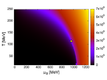
Figure 1: (color online). The temperature and chemical potential dependences of the number density in the PNJL model. The star is the critical end point (CEP) $(T^{\rm CEP},\mu^{\rm CEP}_{B})\simeq(114,965)$ [MeV].

III Numerical results

III.1 Exact results in the PNJL model

Figure 1 shows the exact results of the real baryon number density $n_{B}=n_{q}/3$ depending on temperature and baryon chemical potential $(\mu_{B}=3\mu)$ in the PNJL model. The critical end point (CEP): $(T^{\rm CEP},\mu^{\rm CEP}_{B})\simeq(114,965)$ [MeV] is represented as a star in Fig. 1. These results are close to the previously obtained results Fukushima:2003fw , and will be compared with the results in the following subsections.

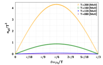
Figure 2: (color online). The $\theta$ dependence of the imaginary number density in the PNJL model.

Table 1: The coefficients $f_{3k}$ from the data of $n_{qI}/T^{3}$ for each temperature.

$T$ [MeV]	$f_{3}$	$f_{6}$	$f_{9}$	$f_{12}$
200	$2.2\times 10^{-2}$	$1.7\times 10^{-4\ }$	$1.9\times 10^{-6\ }$	$2.2\times 10^{-8\ }$
160	$5.5\times 10^{-3}$	$9.0\times 10^{-6\ }$	$2.1\times 10^{-8\ }$	$5.8\times 10^{-11}$
120	$7.2\times 10^{-4}$	$9.9\times 10^{-8\ }$	$2.0\times 10^{-11}$	$4.7\times 10^{-15}$
80	$1.4\times 10^{-5}$	$1.7\times 10^{-11}$	$3.0\times 10^{-17}$	—

III.2 Imaginary number density in the PNJL model

We evaluate the imaginary number density $n_{qI}$ at the pure imaginary chemical potential from Eq. (LABEL:nq). The momentum integrations in Eqs. (LABEL:Mgap), (LABEL:rgap) and (LABEL:pgap) are calculated with the Gaussian quadrature method. Figure 2 shows the $\theta$ (=$\mu_{I}/T$) dependence of the imaginary number density. $n_{qI}/T^{3}$ are calculated at 161 values of $\mu_{I}$ for various temperatures. The PNJL model has the $Z_{3}$ symmetry and an anti-symmetry such as $n_{qI}(\theta)=n_{qI}(\theta+2\pi/3)$ and $n_{qI}(\theta)=-n_{qI}(-\theta)$. Therefore, we only show the region $0\leq\theta\leq\pi/3$ in Fig. 2. From Fig. 2, we find that $n_{qI}$ is well approximated by the Fourier series

$$\frac{n_{qI}}{T^{3}}(\theta) = \sum_{k=1}^{N_{{\sin}}}f_{3k}\sin(3k\theta)\ ,$$ (19)

which is used instead of Eq. (4) since $f_{k}$ for $\mod(k,3)\neq 0$ are zero due to the $Z_{3}$ symmetry. Since we are interested in the confinement phase of QCD here, the $Z_{3}$ symmetric feature in Eq. (19) remains intact. The obtained coefficients $f_{3k}$ are listed in Table 1.

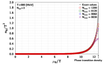
Figure 3: (color online). The $N_{\rm max}$ dependence of the number density in the PNJL model. The solid line is the exact number density calculated at the real chemical potential. The other symbols are the number densities obtained from the canonical approach for several $N_{\rm max}$.

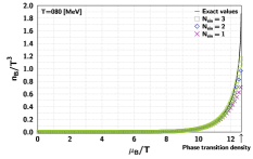
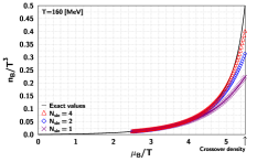
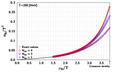
Figure 4: (color online). The $N_{\sin}$ dependence of $n_{B}/T^{3}$ in the PNJL model. The solid lines are the exact number densities calculated at the real chemical potential.

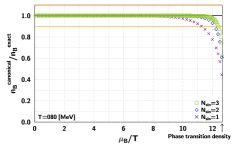
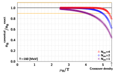
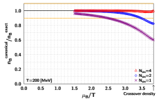
Figure 5: (color online). The $N_{\sin}$ dependence of $n_{B}^{\rm canonical}/n_{B}^{\rm exact}$ in the PNJL model. $n_{B}^{\rm canonical}$ is the number density obtained from the canonical approach and $n_{B}^{\rm exact}$ is the exact number density calculated at the real chemical potential.

III.3 $N_{\rm max}$ dependence of the number density in the PNJL model

Next, we calculate the grand canonical partition function at pure imaginary chemical potential with the integration method in Eq. (5). Here, the finite volume effect is included as the coefficient $V$ in Eq. (5), although the imaginary number densities and $f_{3k}$ in Eq. (19) are computed by the formula for the infinite volume. In this paper, since we study the $N_{\rm max}$ and $N_{\sin}$ dependences of the canonical approach, we use $V=(6\ [{\rm fm}])^{3}$ to minimize the finite $V$ effect, which is justified in comparison with the argument of Ref. Xu:2019gia , where $V\sim(5\ [{\rm fm}])^{3}$ is shown to be sufficiently large.

By performing Fourier transforms in Eq. (2) with 8,192 significant digits in decimal notation, we obtain the canonical partition functions. Finally, we can reconstruct the grand canonical partition function,

$$Z_{\rm GC}(\mu,T,V) = \sum_{n=-N_{\rm max}}^{N_{\rm max}}Z_{C}(n,T,V)\xi^{n}\ ,$$ (20)

where $N_{\rm max}$ is a maximum value of fluctuation of the net quark number in the system. We should take $N_{\rm max}$ to an infinite limit theoretically, but a numerical constraint makes $N_{\rm max}$ finite.

In Fig. 3, we present the $N_{\rm max}$ dependence of the baryon number density $n_{B}$ obtained from the canonical approach at $T=80$ [MeV]. The solid line is the exact number density calculated at the real chemical potential. The figure only shows up to the exact phase transition density because the Fourier transforms in the canonical approach are ineffective over the phase transition point. From Fig. 3, we find that the behavior of the number density converges for $N_{\rm max}=120$ and larger. Note that the difference between $n_{B}$ calculated from the canonical approach and the exact values near the phase transition density comes from the finite $N_{\sin}$ effect, which we discuss in the next subsection. Now we can understand the converging behavior of $n_{B}$ by comparing $N_{\rm max}/(3V)=120/(3\times 6^{3})\sim 0.19$ [fm^-3] with the normal nuclear matter density 0.17 [fm^-3]. It is reasonable to expect that the fluctuations of the number density are in the same order of the nuclear matter density in the region of the chemical potential and temperature that we are looking at now.

III.4 $N_{\sin}$ dependence of the number density in the PNJL model

In this subsection, we discuss the $N_{\sin}$ dependence by using $N_{\rm max}=1200$ to suppress possible uncertainties due to finite $N_{\rm max}$. In Fig. 4, we show the $N_{\sin}$ dependence of the baryon number density at $T=80,$ 160 and 200 [MeV]. The solid lines are the exact number densities $n_{B}^{\rm exact}$ calculated at the real chemical potential. The symbols represent the number densities obtained from the canonical approach, $n_{B}^{\rm canonical}$. As $N_{\sin}$ increases, the difference between $n_{B}^{\rm exact}$ and $n_{B}^{\rm canonical}$ becomes small.

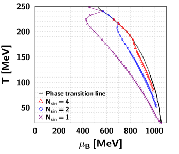
Figure 6: (color online). The boundaries of the effective regions of the canonical approach for $N_{\sin}$ in the PNJL model. The black solid and dashed lines represent the first-order phase transition and crossover lines, respectively. The points of making a 10% difference between the exact $n_{B}$ and the results from the canonical approach are plotted. We plot the symbols on the crossover line when the difference is less than 10% in the confinement phase.

In Fig. 5, we show the $N_{\sin}$ dependence of the ratio of $n_{B}^{\rm canonical}$ to $n_{B}^{\rm exact}$ at $T=80,$ 160 and 200 [MeV]. The solid and dashed lines represent the exact value ($n_{B}^{\rm canonical}/n_{B}^{\rm exact}=1.0$) and the 10% difference values ($n_{B}^{\rm canonical}/n_{B}^{\rm exact}=0.9$ and 1.1), respectively. In this paper, we define the density region having a difference of less than 10% as the effective region of the canonical approach. For $N_{\sin}=1$ at $T=80$, 160 and 200 [MeV], the boundaries of the effective region of the canonical approach appear at the 89%, 74% and 65% of the phase transition or crossover densities, respectively. It turns out that as the temperature decreases, the Fourier series approximation with $N_{\sin}=1$ becomes better. For $N_{\sin}=3$ at $T=80$ [MeV] and $N_{\sin}=4$ at $T=160$ [MeV], we can reconstruct the exact baryon number density from the canonical approach until (97 – 98) % of the phase transition or crossover density within the 10% difference. Moreover, for $N_{\sin}=4$ at $T=200$ [MeV], $n_{B}^{\rm canonical}$ only appears the difference less than 1.8% from the exact value until the crossover density.

In Fig. 6, we plot the symbols on the boundaries of the effective region of the canonical approach for each $N_{\sin}$ and temperature. In the left regions of the boundaries, we can discuss $n_{B}$ within the 10% difference from the canonical approach. When the difference is less than 10% in the confinement phase, we plot the symbols on the crossover density as the high-density limits of the effective region, such as at $T=(184-224)$ [MeV] for $N_{\sin}=4$. The reason is that there is no crossover or phase transition structure in the Fourier series approximation with finite $N_{\sin}$ since the function is analytic. From Fig. 6, we find that most of the confinement phase can be reliably studied by the canonical approach with $N_{\sin}=4$. Furthermore, for $T<T^{\mathrm{CEP}}$ and $\mu_{B}<900$ [MeV], $N_{\sin}=1$ or 2 is enough to reconstruct the exact number density from the canonical approach. The results suggest that the application of the canonical approach to the lattice QCD is useful, especially in the confinement phase.

III.5 Comparison with the NJL and PNJL models

At the end of this section, we consider the model dependence by comparing the results of the PNJL model with those of the NJL one. In the NJL model, we obtain the coefficients $f_{k}$ from 161 values of data of $n_{qI}/T^{3}$ such as Table 2. Here, we use not Eq. (19) but Eq. (4) since the NJL model does not have the $Z_{3}$ symmetry. As it was done in the PNJL model, we set $V$ in Eq. (3) to $(6\ [{\rm fm}])^{3}$ and reconstruct the grand canonical partition function by performing the Fourier transforms with 8,192 significant digits in decimal notation.

Table 2: The coefficients $f_{k}$ from the data of $n_{qI}/T^{3}$ for each temperature in the NJL model.

$T$ [MeV]	$f_{1}$	$f_{2}$	$f_{3}$	$f_{4}$
79	$2.7\times 10^{-1}$	$2.3\times 10^{-3}$	$2.9\times 10^{-5\ }$	$4.2\times 10^{-7\ }$
49	$3.7\times 10^{-2}$	$1.8\times 10^{-5}$	$1.3\times 10^{-8\ }$	$1.1\times 10^{-11}$
29	$6.5\times 10^{-4}$	$1.9\times 10^{-9}$	$7.9\times 10^{-15}$	$3.9\times 10^{-20}$

Figure 7 shows the $N_{\max}$ dependence of the baryon number density at $T=49$ [MeV] in the NJL model. The solid line is the exact number density calculated at the real chemical potential. We find that the behavior of the number density converges for $N_{\rm max}=120$ and larger, which is the same as the result of the PNJL model. In the following discussion for the NJL model, we use $N_{\rm max}=400$.

In Fig. 8, we show the $N_{\sin}$ dependence of the number density at $T=29$, 49 and 79 [MeV] in the NJL model. The solid lines are the exact number densities $n_{B}^{\rm exact}$ calculated at the real chemical potential. The symbols represent the number densities obtained from the canonical approach, $n_{B}^{\rm canonical}$. As $N_{\sin}$ increases, the difference between $n_{B}^{\rm exact}$ and $n_{B}^{\rm canonical}$ becomes small.

In Fig. 9, we show the $N_{\sin}$ dependence of the ratio of $n_{B}^{\rm canonical}$ to $n_{B}^{\rm exact}$ in the NJL model. For $N_{\sin}=4$ at $T=29$, 49 and 79 [MeV], we can reconstruct the exact baryon number density from the canonical approach until 99%, 97% and 96% of the phase transition or crossover density within the 10% difference, respectively.

In Fig. 10, we plot the symbols on the high-density limits of the effective region of the canonical approach for each $N_{\sin}$ and temperature in the NJL model. We find that the effective region of the canonical approach for $N_{\sin}=4$ can cover in most of the confinement phase. For $T\lesssim 49\sim T^{\mathrm{CEP}}$ [MeV] and $\mu_{B}\lesssim 900$ [MeV], $N_{\sin}=1$ or 2 is enough to reconstruct the exact number density from the canonical approach. The results have universality for at least the NJL and PNJL models.

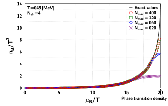
Figure 7: (color online). The $N_{\rm max}$ dependence of the number density in the NJL model. The solid line is the exact number density calculated at the real chemical potential. The other symbols are the number densities obtained from the canonical approach for several $N_{\rm max}$.

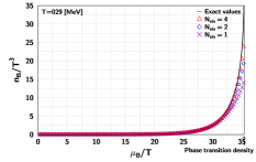
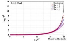
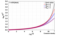
Figure 8: (color online). The $N_{\sin}$ dependence of $n_{B}/T^{3}$ in the NJL model. The solid lines are the exact number densities calculated at the real chemical potential.

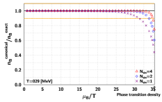
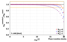
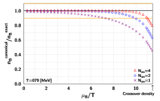
Figure 9: (color online). The $N_{\sin}$ dependence of $n_{B}^{\rm canonical}/n_{B}^{\rm exact}$ in the NJL model. $n_{B}^{\rm canonical}$ is the number density obtained from the canonical approach and $n_{B}^{\rm exact}$ is the exact number density calculated at the real chemical potential.

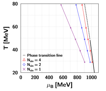
Figure 10: (color online). The boundaries of the effective regions of the canonical approach for $N_{\sin}$ in the NJL model. The black solid and dashed lines represent the first-order phase transition and crossover lines, respectively. The points of making a 10% difference between the exact $n_{B}$ and the results from the canonical approach are plotted.

IV Summary

We have investigated the effective region of the canonical approach in the NJL and PNJL models. We have calculated the 161 data of the imaginary number densities as functions of the pure imaginary chemical potential. By using the integration method of a Fourier series with finite $N_{\sin}$ for the imaginary number densities and performing Fourier transforms with the multiple-precision arithmetic, we have reconstructed the grand canonical partition function, which is written as a fugacity expansion with finite $N_{\rm max}$. After that, we have calculated the number densities at the real chemical potential from the grand canonical partition function. Because the number densities are already known in the NJL and PNJL models, we can clarify the region where the canonical approach works well by comparing the number densities obtained from the canonical approach with the exact ones.

We have shown the $N_{\rm max}$ and $N_{\sin}$ dependences of the number densities obtained from the canonical approach in each model. In the investigation of the $N_{\rm max}$ dependence, we have found that the finite $N_{\rm max}$ effect for the number density is suppressed for the maximum value of the fluctuation of the net quark number density in the system, $N_{\rm max}/V$, larger than 0.56 [fm^-3].

For the $N_{\sin}$ dependence, we have found that the results for $N_{\sin}$ up to 4 can reconstruct the exact number density from the canonical approach until 96% of the phase transition or crossover density within the 10% difference. Moreover, $N_{\sin}=1$ or 2 is enough to reconstruct the exact number density within the 10% difference for $T<T^{\mathrm{CEP}}$ and $\mu_{B}<900$ [MeV]. The results have universality for at least the NJL and PNJL models. They suggest that the application of the canonical approach to the lattice QCD is useful, especially in the confinement phase.

In this paper, we have discussed the effective region of the canonical approach for the number density in the NJL and PNJL models. It remains to be investigated for other physical quantities and other models.

- (1) A. Hasenfratz and D. Toussaint, “Canonical ensembles and nonzero density quantum chromodynamics,” Nucl. Phys. B 371, 539 (1992).
- (2) K. Morita, V. Skokov, B. Friman and K. Redlich, “Net baryon number probability distribution near the chiral phase transition,” Eur. Phys. J. C 74, 2706 (2014) [arXiv:1211.4703 [hep-ph]].
- (3) R. Fukuda, A. Nakamura and S. Oka, “Canonical approach to finite density QCD with multiple precision computation,” Phys. Rev. D 93, no. 9, 094508 (2016) [arXiv:1504.06351 [hep-lat]].
- (4) A. Nakamura, S. Oka and Y. Taniguchi, “QCD phase transition at real chemical potential with canonical approach,” JHEP 1602, 054 (2016) [arXiv:1504.04471 [hep-lat]].
- (5) P. de Forcrand and S. Kratochvila, “Finite density QCD with a canonical approach,” Nucl. Phys. Proc. Suppl. 153, 62 (2006) [hep-lat/0602024].
- (6) S. Ejiri, “Canonical partition function and finite density phase transition in lattice QCD,” Phys. Rev. D 78, 074507 (2008) [arXiv:0804.3227 [hep-lat]].
- (7) A. Li, A. Alexandru, K. F. Liu and X. Meng, “Finite density phase transition of QCD with and using canonical ensemble method,” Phys. Rev. D 82, 054502 (2010) [arXiv:1005.4158 [hep-lat]].
- (8) A. Li, A. Alexandru and K. F. Liu, “Critical point of QCD from lattice simulations in the canonical ensemble,” Phys. Rev. D 84, 071503 (2011) [arXiv:1103.3045 [hep-ph]].
- (9) J. Danzer and C. Gattringer, “Properties of canonical determinants and a test of fugacity expansion for finite density lattice QCD with Wilson fermions,” Phys. Rev. D 86, 014502 (2012) [arXiv:1204.1020 [hep-lat]].
- (10) C. Gattringer and H. P. Schadler, “Generalized quark number susceptibilities from fugacity expansion at finite chemical potential for = 2 Wilson fermions,” Phys. Rev. D 91, no. 7, 074511 (2015) [arXiv:1411.5133 [hep-lat]].
- (11) D. L. Boyda, V. G. Bornyakov, V. A. Goy, V. I. Zakharov, A. V. Molochkov, A. Nakamura and A. A. Nikolaev, “Novel approach to deriving the canonical generating functional in lattice QCD at a finite chemical potential,” JETP Lett. 104, no. 10, 657 (2016) [Pisma Zh. Eksp. Teor. Fiz. 104, no. 10, 673 (2016)].
- (12) V. A. Goy, V. Bornyakov, D. Boyda, A. Molochkov, A. Nakamura, A. Nikolaev and V. Zakharov, “Sign problem in finite density lattice QCD,” PTEP 2017, no. 3, 031D01 (2017) [arXiv:1611.08093 [hep-lat]].
- (13) V. G. Bornyakov, D. L. Boyda, V. A. Goy, A. V. Molochkov, A. Nakamura, A. A. Nikolaev and V. I. Zakharov, “New approach to canonical partition functions computation in lattice QCD at finite baryon density,” Phys. Rev. D 95, no. 9, 094506 (2017) [arXiv:1611.04229 [hep-lat]].
- (14) D. Boyda, V. G. Bornyakov, V. Goy, A. Molochkov, A. Nakamura, A. Nikolaev and V. I. Zakharov, “Lattice QCD thermodynamics at finite chemical potential and its comparison with Experiments,” arXiv:1704.03980 [hep-lat].
- (15) M. Wakayama, V. G. Borynakov, D. L. Boyda, V. A. Goy, H. Iida, A. V. Molochkov, A. Nakamura and V. I. Zakharov, “Lee-Yang zeros in lattice QCD for searching phase transition points,” Phys. Lett. B 793, 227 (2019) [arXiv:1802.02014 [hep-lat]].
- (16) M. Wakayama and A. Hosaka, “Search of QCD phase transition points in the canonical approach of the NJL model,” Phys. Lett. B 795, 548 (2019) [arXiv:1905.10956 [hep-lat]].
- (17) Y. Nambu and G. Jona-Lasinio, “Dynamical Model of Elementary Particles Based on an Analogy with Superconductivity. 1.,” Phys. Rev. 122, 345 (1961).
- (18) Y. Nambu and G. Jona-Lasinio, “Dynamical Model Of Elementary Particles Based On An Analogy With Superconductivity. Ii,” Phys. Rev. 124, 246 (1961).
- (19) T. Kunihiro, “Quark number susceptibility and fluctuations in the vector channel at high temperatures,” Phys. Lett. B 271, 395 (1991).
- (20) T. Hatsuda and T. Kunihiro, “QCD phenomenology based on a chiral effective Lagrangian,” Phys. Rept. 247, 221 (1994) [hep-ph/9401310].
- (21) K. Fukushima, “Chiral effective model with the Polyakov loop,” Phys. Lett. B 591, 277 (2004) [hep-ph/0310121].
- (22) S. Roessner, T. Hell, C. Ratti and W. Weise, “The chiral and deconfinement crossover transitions: PNJL model beyond mean field,” Nucl. Phys. A 814, 118 (2008) [arXiv:0712.3152 [hep-ph]].
- (23) M. D’Elia and F. Sanfilippo, “Thermodynamics of two flavor QCD from imaginary chemical potentials,” Phys. Rev. D 80, 014502 (2009) [arXiv:0904.1400 [hep-lat]].
- (24) T. Takaishi, P. de Forcrand and A. Nakamura, “Equation of State at Finite Density from Imaginary Chemical Potential,” PoS LAT 2009, 198 (2009) [arXiv:1002.0890 [hep-lat]].
- (25) V. Skokov, B. Friman and K. Redlich, “Quark number fluctuations in the Polyakov loop-extended quark-meson model at finite baryon density,” Phys. Rev. C 83, 054904 (2011) [arXiv:1008.4570 [hep-ph]].
- (26) D. M. Smith, Multiple Precision Computation, FMLIB1.3 (2015). http://myweb.lmu.edu/dmsmith/FMLIB.html.
- (27) K. Xu and M. Huang, “Zero-mode contribution and quantized first order phase transition in a droplet quark matter,” arXiv:1903.08416 [hep-ph].