Dependence of the surface tension and contact angle on the temperature,
as described by the diffuse-interface model

Abstract

Four results associated with the diffuse-interface model (DIM) for contact lines are reported in this paper. First, a boundary condition is derived, which states that the fluid near a solid wall must have a certain density $\rho_{0}$ depending on the solid’s properties. Unlike previous derivations, the one presented here is based on the same physics as the DIM itself and does not require additional assumptions. Second, asymptotic estimates are used to check a conjecture lying at the foundation of the DIM, as well as all other models of contact lines: that liquid–vapor interfaces are nearly isothermal. It turns out that, for water, they are not – although, for a more viscous fluid, they can be. The non-isothermaility occurs locally, near the interface, but can still affect the contact-line dynamics. Third, the DIM coupled with a realistic equation of state for water is used to compute the dependence of the surface tension $\sigma$ on the temperature $T$, which agrees well with the empiric $\sigma(T)$. Fourth, the same framework is used to compute the static contact angle of a water–vapor interface. It is shown that, with increasing temperature, the contact angle becomes either $180^{\circ}$ (perfect hydrophobicity) or $0^{\circ}$ (perfect hydrophilicity), depending on whether $\rho_{0}$ matches the density of saturated vapor or liquid, respectively. Such behavior presumably occurs in all fluids, not just water, and for all sufficiently strong variations of parameters, not just that of the temperature – as corroborated by existing observations of drops under variable electric field.

I Introduction

The diffuse-interface model (DIM) [1, 2, 3, 4] is based on an assumption that the van der Waals force in fluids can be described by a pair-wise potential exerted by the molecules on each other. If the potential’s spatial scale is much shorter than that of the flow, the force term in the governing equations can be simplified, yielding the so-called Korteweg stress [5]. The resulting model provides a tool for studying flows involving contact lines, i.e., curves where the gas, liquid, and solid are in simultaneous contact. To this end, one also needs a boundary condition for fluid–solid interfaces, of which several versions exist in the literature. Firstly, Ref. [6] suggested a condition prescribing the density gradient in the direction normal to the solid boundary; secondly, Ref. [3] put forward a condition prescribing a linear combination of the density gradient and the density itself. It was also conjectured in Ref. [3] that, if the solid–fluid interaction is short-ranged by comparison with the fluid–fluid one, the general boundary condition can be simplified, so that just the density is prescribed. This simplest boundary condition is usually employed in applications (e.g., Refs. [7, 8, 9, 10, 11] and references therein).

Curiously, there is only one work, Ref. [12], where the DIM is coupled with a realistic equation of state (EoS). The one used in most other papers is inconsistent with the ideal-gas limit and does not involve temperature (the latter amounts to spatial isothermality). It allows one, however, to find analytically the profile of the liquid–vapor interface, which comes handy when calculating the flow’s macroscopic characteristics (the surface tension and contact angle). Still, the use of a non-realistic EoS renders the DIM somewhat phenomenological rather than physics-based.

A model close to, but still not quite, realistic was examined in Ref. [13], where the DIM was coupled with the van der Waals EoS. Interestingly, simulations carried out in this work showed that interfacial flows can be significantly non-isothermal. This conclusion was confirmed in Ref. [14] by fitting the van der Waals EoS to several specific fluids including water and considering the resulting asymptotic models.

The discrepancies associated with non-realistic equations of state are resolved in the present work. It concentrates on water – not only because of the importance of this fluid, but also because its parameters are well researched, making it easy to verify theoretical results.

In Sects. II-III, the simplest version of the boundary condition (the one conjectured in Ref. [3]) will be derived without assuming that the solid–fluid interactions are short-ranged by comparison with the fluid–fluid ones. It is also shown that, if the DIM is coupled with a realistic EoS for water, it predicts that interfaces are not isothermal, which confirms the results of Ref. [14]. In Sects. IV-V, the DIM is used to calculate the dependence of the surface tension and contact angle on the temperature (both for water).

II Formulation

II.1 Basic thermodynamics of non-ideal fluids

Let $\rho$ be the mass density of a fluid, and $s$ and $e$ be the entropy and internal energy (both per unit mass), respectively. Then, the fluid’s properties are fully determined by the function $e(\rho,s)$; the temperature $T$ and pressure $p$, for example, are given by

$$T=\left(\frac{\partial e}{\partial s}\right)_{\rho},\qquad p=\rho^{2}\left(\frac{\partial e}{\partial\rho}\right)_{s},$$ (1)

where, as usual, the subscripts imply that the corresponding variables are held constant.

Instead of using $s$ as one of the primary thermodynamic variables, it is more convenient to use $T$. Rewriting the first equality of (1) in terms of $\left(\rho,T\right)$, one obtains a restriction linking allowable $e(\rho,T)$ and $s(\rho,T)$,

$$\left(\dfrac{\partial e}{\partial T}\right)_{\rho}=T\left(\dfrac{\partial s}{\partial T}\right)_{\rho}.$$ (2)

Rewriting the second equality of (1) and taking into account (2), one obtains the EoS,

$$p=-T\rho^{2}\left(\dfrac{\partial s}{\partial\rho}\right)_{T}-a\rho^{2},$$ (3)

where

$$a=-\left(\frac{\partial e}{\partial\rho}\right)_{T},$$ (4)

can be interpreted as the first van der Waals parameter – but, unlike its classical counterpart, it may depend on $\rho$ and $T$.

Introduce also the specific heat capacity

$$c_{V}=\left(\frac{\partial e}{\partial T}\right)_{\rho}$$

and the Gibbs free energy

$$G=e-Ts+\frac{p}{\rho}.$$ (5)

Using (2)-(3), one can show that $G$ is related to the pressure by

$$\left(\dfrac{\partial G}{\partial\rho}\right)_{T}=\frac{1}{\rho}\left(\frac{\partial p}{\partial\rho}\right)_{T}.$$ (6)

The general results in this work will be illustrated using the Enskog–Vlasov (EV) equation of state, resulting from the hydrodynamic approximation of the EV kinetic equation [15, 16, 17, 18] and implying

$$e=c_{V}T-a\rho,\qquad s=c_{V}\ln T-R\ln\rho-R\,\Theta(b\rho),$$ (7)

where $c_{V}$ and $a$ are independent of $\rho$ and $T$, $R$ is the specific gas constant, $b$ is the EV equivalent of the second van der Waals parameter, and $\Theta(\xi)$ (with $\xi=b\rho$) is a fluid-specific function describing the non-ideal part of the entropy. Substitution of (7) into (3) yields

$$p=RT\rho\left[1+b\rho\,\Theta^{\prime}(b\rho)\right]-a\rho^{2},$$ (8)

where $\Theta^{\prime}(\xi)=\mathrm{d}\Theta(\xi)/\mathrm{d}\xi$. Note that, in applications of the EV theory to real fluids [17, 18], the best choice for $b$ turned out to be the reciprocal of the fluid’s triple-point density.

Observe that Eq. (8) includes the van der Waals EoS as a particular case with $\Theta(\xi)=-\ln\left(1-\xi\right)$.

II.2 The governing equations and boundary conditions

Traditionally, the diffuse-interface model is introduced through the free energy of fluid–fluid and solid–fluid interactions [3]. It seems simpler, however, to do so through pair-wise forces exerted by the fluid molecules on each other, and the forces exerted on the molecules by the (solid) walls.

Let the former forces be described by an isotropic potential $\Phi(r)$ ($r$ is the distance between the interacting molecules) and the latter, by a potential $U(\mathbf{r})$ which decays rapidly when $\mathbf{r}$ moves away from the wall.

Introducing the molecular mass $m$ (so that $\rho/m$ is the number density), one can express the total collective force in the form

$$\mathbf{F}(\mathbf{r},t)=-\frac{\rho(\mathbf{r},t)}{m}\\ \times\pmb{\pmb{\nabla}}\left[\int_{\mathcal{D}}\frac{\rho(\mathbf{r}_{1},t)}{m}\Phi(\left|\mathbf{r-r}_{1}\right|)\,\mathrm{d}^{3}\mathbf{r}_{1}+U(\mathbf{r})\right],$$ (9)

where $\mathcal{D}$ is the domain occupied by the fluid (physically, the container).

A compressible Newtonian fluid affected by a force $\mathbf{F}$ is governed by [19]

$$\frac{\partial\rho}{\partial t}+\pmb{\pmb{\nabla}}\cdot\left(\rho\mathbf{v}\right)=0,$$ (10)

$$\frac{\partial\mathbf{v}}{\partial t}+\left(\mathbf{v}\cdot\pmb{\pmb{\nabla}}\right)\mathbf{v}+\frac{1}{\rho}\pmb{\pmb{\nabla}}\cdot\left(\mathbf{I}\,p-\pmb{\Pi}\right)=\frac{1}{\rho}\mathbf{F},$$ (11)

$$\rho c_{V}\left(\frac{\partial T}{\partial t}+\mathbf{v}\cdot\pmb{\pmb{\nabla}}T\right)+\left[\mathbf{I}\left(p+a\rho^{2}\right)-\pmb{\Pi}\right]:\pmb{\pmb{\nabla}}\mathbf{v}\\ -\pmb{\pmb{\nabla}}\cdot\left(\kappa\pmb{\pmb{\nabla}}T\right)=0.$$ (12)

where $\mathbf{I}$ is the identity matrix,

$$\pmb{\Pi}=\mu_{s}\left[\pmb{\pmb{\nabla}}\mathbf{v}+\left(\pmb{\pmb{\nabla}}\mathbf{v}\right)^{T}-\frac{2}{3}\mathbf{I}\left(\pmb{\pmb{\nabla}}\cdot\mathbf{v}\right)\right]+\mu_{b}\,\mathbf{I}\left(\pmb{\pmb{\nabla}}\cdot\mathbf{v}\right),$$ (13)

is the viscous stress tensor, $\mu_{s}$ ($\mu_{b}$) is the shear (bulk) viscosity, and $\kappa$, the thermal conductivity.

Observe that the governing equations (9)-(12) are invariant with respect to the simultaneous substitution

$$\Phi(r)=\Phi_{new}(r)+C\,\delta(\mathbf{r}),$$ (14)

$$p=p_{new}-\frac{C}{2m^{2}}\rho^{2},\qquad a=a_{new}+\frac{C}{2m^{2}},$$ (15)

where $\delta(\mathbf{r})$ is the Dirac delta-function and $C$ is an arbitrary constant. Furthermore, recalling (3)-(4), one can see that substitutions (15) both correspond to

$$e=e_{new}-\frac{C}{2m^{2}}\rho.$$

Choosing in (14) an appropriate value of $C$, one can make $\Phi_{new}$ satisfy (the subscript _new omitted)

$$\int\Phi(r)\,\mathrm{d}^{3}\mathbf{r}=0,$$ (16)

where integration is to be carried out over the whole space. In what follows, the so-called Korteweg parameter will be needed, given by

$$K=-\frac{1}{m^{2}}\int r^{2}\Phi(r)\,\mathrm{d}^{3}\mathbf{r}.$$ (17)

At $\partial\mathcal{D}$ (the container walls), Eqs. (9)-(13) should be complemented by the no-flow condition,

$$\mathbf{v}=\mathbf{0}\qquad\text{at}\qquad\mathbf{r}\in\partial\mathcal{D},$$ (18)

and a boundary condition for the temperature. The latter does not play a role in this work, so it is not discussed.

Most importantly, the governing equations do not require a boundary condition for the density  (as the term $\mathbf{v}\cdot\pmb{\pmb{\nabla}}\rho$ in Eq. (10) vanishes at $\mathbf{r}\in\partial\mathcal{D}$ due to (18), and the other equations do not involve derivatives of $\rho$).

II.3 Nondimensionalization

Let $\bar{r}$ be the spatial scale of the flow and $\bar{v}$, its characteristic velocity, so the time scale is $\bar{r}/\bar{v}$. The density will be scaled by its triple-point value (denoted by $b^{-1}$, with a view of using the EV EoS later); the pressure will be scaled by $b^{-2}\bar{a}$ [where $\bar{a}\$is the characteristic value of $a(\rho,T)$]; and the temperature, by a characteristic value $\bar{T}$.

The following nondimensional variables will be used:

$$\mathbf{r}_{nd}=\frac{\mathbf{r}}{\bar{r}},\qquad t_{nd}=\frac{\bar{v}}{\bar{r}}t,$$

$$\rho_{nd}=b\rho,\qquad\mathbf{v}_{nd}=\frac{\mathbf{v}}{\bar{v}},\qquad p_{nd}=\frac{b^{2}}{\bar{a}}p,\qquad T_{nd}=\frac{T}{\bar{T}}.$$

It is convenient to also introduce the nondimensional versions of the fluid parameters. Assume for simplicity that the bulk and shear viscosities are of the same order ($\sim\bar{\mu}$) and denote the other two scales by $\bar{\kappa}$ and $\bar{c}_{V}$, so that

$$\left(\mu_{s}\right)_{nd}=\frac{\mu_{s}}{\bar{\mu}},\qquad\left(\mu_{b}\right)_{nd}=\frac{\mu_{b}}{\bar{\mu}},\qquad\kappa_{nd}=\frac{\kappa}{\bar{\kappa}},$$

$$\left(c_{V}\right)_{nd}=\frac{c_{V}}{\bar{c}_{V}},\qquad a_{nd}=\frac{a}{\bar{a}}.$$

Then the nondimensional viscous stress is

$$\pmb{\Pi}_{nd}=\frac{\bar{r}}{\bar{\mu}\bar{v}}\pmb{\Pi}.$$

As shown in Sect. IV.3 below, the spatial scale of a static interface is

$$\bar{r}=\left(\frac{K}{\bar{a}}\right)^{1/2},$$

which should also apply to a moving one. Such a scaling makes the van der Waals force comparable, but not necessarily equal, to the pressure gradient. One should also require that the viscous stress be comparable to the pressure gradient (as done in the lubrication approximation), which implies

$$\bar{v}=\frac{\bar{a}\bar{r}}{\bar{\mu}b^{2}}.$$

Physically, $\bar{v}$ characterizes a flow due to a disbalance between the van der Waals force and the pressure gradient (typically, resulting from the interface being curved) – whereas the global flow can have a very different velocity scale.

The DIM is based on an assumption that the spatial scale of $\Phi(r)$ is much smaller than that of the flow: the latter is $\bar{r}$, so let the former be $\varepsilon\bar{r}$ with $\varepsilon\ll 1$. The scale separation allows one to approximate the fluid–fluid interaction by the so-called Korteweg stress – accordingly, it is convenient to scale $\Phi$ using the Korteweg parameter (17):

$$\Phi(r)=\frac{Km^{2}}{\varepsilon^{5}\bar{r}^{5}}\Phi_{nd}(\varepsilon^{-1}r_{nd}),$$

where the factor of $\varepsilon^{5}$ is inserted to make the nondimensional version of the Korteweg parameter equal unity,

$$\int\left(\varepsilon^{-1}r_{nd}\right)^{2}\Phi_{nd}(\varepsilon^{-1}r_{nd})\,\mathrm{d}^{3}(\varepsilon^{-1}\mathbf{r}_{nd})=1.$$ (19)

The solid–fluid potential will be scaled so that the two terms on the right-hand side of (9) are comparable – which amounts to

$$U(\mathbf{r})=\frac{Km}{\varepsilon^{5}\bar{r}^{2}b}U_{nd}(\varepsilon^{-1}\mathbf{r}_{nd}).$$

In terms of the nondimensional variables, Eqs. (9)-(13) have the form (the subscript _nd omitted):

$$\frac{\partial\rho}{\partial t}+\pmb{\pmb{\nabla}}\cdot\left(\rho\mathbf{v}\right)=0,$$ (20)

$$\framebox{$\alpha$}\left[\frac{\partial\mathbf{v}}{\partial t}+\left(\mathbf{v}\cdot\pmb{\pmb{\nabla}}\right)\mathbf{v}\right]+\frac{1}{\rho}\pmb{\pmb{\nabla}}\cdot\left(\mathbf{I}\,p-\pmb{\Pi}\right)\\ =-\frac{1}{\varepsilon^{5}}\pmb{\pmb{\nabla}}\left[\int_{\mathcal{D}}\rho(\mathbf{r}_{1},t)\,\Phi(\varepsilon^{-1}\left|\mathbf{r-r}_{1}\right|)\,\mathrm{d}^{3}\mathbf{r}_{1}\right.\\ \mathbf{+}\left.U(\varepsilon^{-1}\mathbf{r})\vphantom{\int_{\mathcal{D}}}\right],$$ (21)

$$\framebox{$\alpha\gamma$}\rho c_{V}\left(\frac{\partial T}{\partial t}+\mathbf{v}\cdot\pmb{\pmb{\nabla}}T\right)+\framebox{$\beta$}\left[\mathbf{I}\left(p+a\rho^{2}\right)-\pmb{\Pi}\right]:\pmb{\pmb{\nabla}}\mathbf{v}\\ -\pmb{\pmb{\nabla}}\cdot\left(\kappa\pmb{\pmb{\nabla}}T\right)=0,$$ (22)

where $\pmb{\Pi}$ is still given by (13) and

$$\alpha=\frac{K}{\bar{\mu}^{2}b^{3}},\qquad\beta=\dfrac{\bar{a}K}{\bar{\mu}\bar{\kappa}\bar{T}b^{4}},\qquad\gamma=\frac{\bar{c}_{V}\bar{\mu}}{\bar{\kappa}}.$$ (23)

As follows from the positions of $\alpha$ and $\beta$ in Eqs. (21)-(22), the former is the Reynolds number and the latter is an ‘isothermality parameter’ controlling the production of heat by compressibility and viscosity (if $\beta\ll 1$, the flow is close to isothermal). $\gamma$, in turn, is the Prandtl number.

Finally, one can rewrite (16) and (19) in the form

$$\int\Phi(r_{1})\,\mathrm{d}^{3}\mathbf{r}_{1}=0,\qquad\int r_{1}^{2}\Phi(r_{1})\,\mathrm{d}^{3}\mathbf{r}_{1}=1,$$ (24)

where $\mathbf{r}_{1}=\varepsilon^{-1}\mathbf{r}_{nd}$.

III Asymptotic estimates

III.1 The nondimensional parameters

In this subsection, the nondimensional parameters $\alpha$, $\beta$, and $\gamma$ will be estimated for water.

Note that ‘our’ $\bar{a}$ and $b$, are similar to, but not the same as, those in the van der Waals EoS. The latter are defined by fitting the EoS to the parameters of the critical point, making the result inaccurate at room temperature.

In this work, $\bar{a}$ and $b$ were determined through the Enskog–Vlasov EoS, which is much more flexible than its van der Waals counterpart. The details can be found in Appendix A, together with $\bar{a}$ and $b$ given by (57)-(58), respectively. The Korteweg parameter $K$, in turn, is estimated in Sect. IV and given by (42).

To estimate $\alpha$, $\beta$, and $\gamma$, one also needs the characteristic heat capacity $\bar{c}_{V}$, viscosity $\bar{\mu}$, and thermal conductivity $\bar{\kappa}$. In the context of interfacial dynamics, it is reasonable to determine these parameters as the average of those for liquid and vapor. Assuming the temperature of $\bar{T}=25~{}\mathrm{C}^{\circ}$ and using the data from Sect. 6.1 of Ref. [20], one obtains

$$\bar{c}_{V}=2.7892~{}\mathrm{kJ~{}kg}^{-1}\mathrm{K}^{-1},$$

$$\bar{\mu}=449.87~{}\mathrm{\mu Pa~{}s},\qquad\bar{\kappa}=312.45~{}\mathrm{mW~{}m}^{-1}\mathrm{K}^{-1}.$$

Substituting these values, into (23), one obtains

$$\alpha\approx 0.121,\qquad\beta\approx 1.234,\qquad\alpha\gamma\approx 0.486.$$

Interestingly, the estimates of the above parameters based on the (much less accurate) van der Waals EoS [14] yield comparable values: $\alpha\approx 0.143$, $\beta\approx 0.711$, and $\alpha\gamma\approx 0.880$.

It is also worth mentioning that, with increasing $\bar{T}$, the Reynolds number $\alpha$ grows – i.e., high-temperature interfacial flows may be close to inviscid. The isothermality parameter $\beta$, in turn, decreases, but never becomes small – not even when the temperature approaches its critical value. For $\bar{T}=360^{\circ}\mathrm{C}$, for example,

$$\alpha\approx 13.3,\qquad\beta\approx 0.581,\qquad\alpha\gamma\approx 6.60.$$

Thus, interfaces in water are generally non-isothermal due to the heat production by viscosity and compressibility. Even though this effect is local – i.e., occurs near the interface – it can strongly affect the dynamics of contact lines.

In what follows, only moderate (room) temperatures will be considered, corresponding to the following asymptotic regime:

$$\alpha\ll 1,\qquad\beta\sim 1,\qquad\gamma\sim 1.$$ (25)

Other regimes, arising for other fluids, have been examined in Ref. [14] using the van der Waals EoS. Eight fluids were considered (acetone, benzene, ethanol, ethylene glycol, glycerol, mercury, methanol, and water), and only for ethylene glycol and glycerol $\beta$ has turned out to be small. Thus, non-isothermality of liquid–vapor interfaces is likely to be a rule rather than an exception.

III.2 The asymptotic equations

The density equation (20), does not involve any parameters and, thus, remains as is.

Assuming limit (25) and omitting small terms from the temperature equation (22), one obtains

$$\beta\left[\mathbf{I}\left(p+a\rho^{2}\right)-\pmb{\Pi}\right]:\pmb{\pmb{\nabla}}\mathbf{v-}\pmb{\pmb{\nabla}}\cdot\left(\kappa\pmb{\pmb{\nabla}}T\right)=0.$$

The first term in this equation describes production of heat due to compressibility and viscosity, and the second term describes redistribution (diffusion) of the produced heat.

The asymptotic form of the velocity equation depends on whether or not $\mathbf{r}$ is close to a wall.

First, consider the outer region, i.e., far from walls, where the wall-induced potential $U(\mathbf{r})$ can be neglected and the fluid–fluid interaction term can be rearranged as follows:

$$\int_{\mathcal{D}}\rho(\mathbf{r}_{1},t)\,\Phi(\varepsilon^{-1}\left|\mathbf{r-r}_{1}\right|)\,\mathrm{d}^{3}\mathbf{r}_{1}\\ =\varepsilon^{3}\rho(\mathbf{r},t)\int\Phi(r_{1})\,\mathrm{d}^{3}\mathbf{r}_{1}\\ +\varepsilon^{5}\left[\nabla^{2}\rho(\mathbf{r},t)\right]\int r_{1}^{2}\,\Phi(r_{1})\,\mathrm{d}^{3}\mathbf{r}_{1}+\mathcal{O}(\varepsilon^{7}).$$

Taking into account (24), and omitting the small terms, one can rewrite Eq. (21) in the form

$$\frac{1}{\rho}\,\pmb{\pmb{\nabla}}\cdot\left(\mathbf{I}p-\pmb{\Pi}\right)=\pmb{\pmb{\nabla}}\nabla^{2}\rho,$$ (26)

or equivalently

$$\pmb{\pmb{\nabla}}\cdot\left(\mathbf{I}p-\pmb{\Pi}\right)=\pmb{\pmb{\nabla}}\cdot\left[\mathbf{I}\left(\rho\nabla^{2}\rho+\frac{1}{2}\left|\mathbf{\nabla}\rho\right|^{2}\right)-\left(\pmb{\pmb{\nabla}}\rho\right)\left(\pmb{\pmb{\nabla}}\rho\right)\right],$$ (27)

where the expression in the square brackets is the Korteweg stress.

Most importantly, the fluid–fluid interaction term in Eq. (26) is differential – hence, a boundary condition for $\rho$ is needed. It will be derived by matching the outer solution to that in the inner (near-wall) region.

Next, consider the inner region of characteristic thickness $\varepsilon$. Assuming for simplicity that the wall passes through the origin of the coordinate system and is tangent to the $\left(x,y\right)$ plane (so that $U$ depends locally only on $z$), one can neglect the curvature of the inner layer and introduce the inner coordinate $\hat{z}=\varepsilon^{-1}z$. The dependence on $x$ and $y$, in turn, is forced by the outer flow – hence, these variables do not need rescaling except when they appear in $\Phi$, which depends on $\hat{r}=\left(\hat{x}^{2}+\hat{y}^{2}+\hat{z}^{2}\right)^{1/2}$ where $\hat{x}=\varepsilon^{-1}x$ and $\hat{y}=\varepsilon^{-1}y$.

As for the unknowns, the density does not need rescaling, but the velocity does, as the no-flow boundary condition (18) suggest $\mathbf{\hat{v}}=\mathbf{v}/\varepsilon$. Finally, since the inner region is thin, the temperature there should be assumed to be independent of $\hat{z}$.

One can see that the rescaled version of Eq. (21) is dominated by the fluid–fluid and solid–fluid interactions. Thus, to leading order, one obtains

$$\frac{\partial}{\partial\hat{z}}\left[\int_{0}^{\infty}\rho(\hat{z}_{1})\,\Psi(\hat{z}-\hat{z}_{1})\,\mathrm{d}\hat{z}_{1}+U(\hat{z})\right]=0,$$ (28)

where

$$\Psi(\hat{z})=\int\int\Phi(\hat{r})\,\mathrm{d}\hat{x}\,\mathrm{d}\hat{y}.$$ (29)

Observe that condition (23) and the symmetry of $\Phi(\hat{r})$ imply

$$\int\Psi(\hat{z})\,\mathrm{d}\hat{z}=0,\qquad\int\hat{z}\,\Psi(\hat{z})\,\mathrm{d}\hat{z}=0.$$ (30)

Given (30), one can readily verify that Eq. (28) is consistent with the following long-range behavior:

$$\hat{\rho}(\hat{z})\sim\rho_{0}+\rho_{0}^{\prime}\,\hat{z}+\frac{1}{2}\rho_{0}^{\prime\prime}\,\hat{z}^{2}\qquad\text{as}\qquad\hat{z}\rightarrow\infty,$$ (31)

where $\rho_{0}$, $\rho_{0}^{\prime}$, and $\rho_{0}^{\prime\prime}$ do not depend on $\hat{z}$ (but can depend on $x$, $y$, and $t$).

Asymptotic (31) is to be matched to the outer solution. If $\rho_{0}^{\prime\prime}\neq 0$, (31) implies that the outer solution is such that

$$\frac{\partial^{2}\rho}{\partial z^{2}}=O(\varepsilon^{-2})\qquad\text{as}\qquad z\rightarrow 0,$$

indicating a mismatch unless $\rho_{0}^{\prime\prime}=0$. A similar argument yields $\rho_{0}^{\prime}=0$, so that the boundary condition for the outer solution is

$$\rho=\rho_{0}\qquad\text{at}\qquad\mathbf{r}\in\partial\mathcal{D}.$$ (32)

The parameter $\rho_{0}$ should be calculated by solving Eq. (28) subject to condition (31) with $\rho_{0}^{\prime}=\rho_{0}^{\prime\prime}=0$. Physically, $\rho_{0}$ is determined by a balance between the solid–fluid and fluid–fluid interactions.

An example where Eq. (28) can be solved analytically is given in Appendix B.

III.3 Static interfaces

The rest of this work is concerned with static interfaces, for which $\partial/\partial t=0$ and $\mathbf{v}=\mathbf{0}$. It is also clear that static fluid ought to be isothermal (in all models, both exact and asymptotic), so $T=\operatorname{const}$.

Taking this into account and returning to the dimensional variables, one can write the asymptotic equations (26) in the form

$$\frac{1}{\rho}\,\pmb{\pmb{\nabla}}p=K\pmb{\pmb{\nabla}}\nabla^{2}\rho,$$ (33)

where it is implied that $p$ depends on $\rho$ and, parametrically, on $T$. Equation (33) and the boundary condition (32) fully determine $\rho(\mathbf{r})$.

Eq. (33) can be rewritten in a mathematically equivalent (but, in some cases, more convenient) form. Multiplying (33) by $\rho$ and integrating, one obtains

$$p-p_{0}=K\left(\rho\nabla^{2}\rho-\frac{1}{2}\left|\pmb{\pmb{\nabla}}\rho\right|^{2}\right),$$ (34)

where $p_{0}$ is a constant of integration (and, physically, the pressure at infinity). Alternatively, using identity (6), one can rewrite (33) in terms of the Gibbs free energy,

$$G-G_{0}=K\nabla^{2}\rho,$$ (35)

where $G_{0}$ is a constant of integration (and, physically, the equilibrium value of $G$).

IV The surface tension vs. temperature

IV.1 Theory

It is well known (e.g., [21]) that the surface tension of a liquid–vapor interface can be related to the one-dimensional solution of Eq. (33). To do so, substitute $\rho=\rho_{lv}(z)$ into (33) which yields

$$\frac{1}{\rho_{lv}}\frac{\mathrm{d}p(\rho_{lv},T)}{\mathrm{d}z}=K\frac{\mathrm{d}^{3}\rho_{lv}}{\mathrm{d}z^{3}}.$$ (36)

There are no solid boundaries in this case, thus,

$$\rho \rightarrow\rho_{l}\qquad\text{as}\qquad z\rightarrow-\infty,$$ (37)

$$\rho \rightarrow\rho_{v}\qquad\text{as}\qquad z\rightarrow+\infty,$$ (38)

where $\rho_{l}$ and $\rho_{v}$ are the densities of the liquid and vapor, respectively. Using the one-dimensional reductions of Eqs. (34)-(35), one can show that the boundary-value problem (36)-(38) has a solution only if $\rho_{l}$ and $\rho_{v}$ satisfy the Maxwell construction, i.e., the following algebraic equations:

$$p(\rho_{l},T)=p(\rho_{v},T),\qquad G(\rho_{l},T)=G(\rho_{v},T).$$ (39)

Eqs. (39) determine how $\rho_{l}$ and $\rho_{v}$ depend on $T$; interestingly, they are exact despite the approximate nature of the DIM.

Once the boundary-value problem (36)-(39) is solved and its solution $\rho_{lv}(z)$ is found, the surface tension is given by

$$\sigma=K\int_{-\infty}^{\infty}\left(\frac{\mathrm{d}\rho_{lv}}{\mathrm{d}z}\right)^{2}\mathrm{d}z.$$ (40)

IV.2 Comparison with observations

Before comparing the dependence of $\sigma$ on $T$ determined by (40) to that measured for a specific fluid, one has to specify the EoS and the Korteweg parameter $K$. The former will be approximated by the Enskog–Vlasov EoS (see Appendix A) and the latter is discussed below.

The simplest way to fix $K$ consists in solving the boundary-value problem (36)-(38) for a certain value of $T$ – say, at the triple point – and ensure that the value of $\sigma$ predicted by (40) coincides with the surface tension $\sigma_{r}$ measured for a real liquid–vapor interface. For water, the latter value is [23]

$$\sigma_{r}=75.65\times 10^{-3}\mathrm{N~{}m}^{-1}\hskip 14.22636pt\text{at}\hskip 14.22636ptT=273.16~{}\mathrm{K}.$$ (41)

Eqs. (36)-(39) with the EoS given by (8), (57)-(61) were solved numerically and the computed $\rho_{lv}(z)$ was substituted into (40). The resulting $\sigma$ agrees with (41) if

$$K=2.45\times 10^{-17}\mathrm{m}^{7}\mathrm{kg}^{-1}\mathrm{N}^{-2}.$$ (42)

Now, one can compute $\sigma(T)$ for the whole temperature range where liquid water and vapor coexist, i.e., between the triple and critical points. The theoretical dependence is compared to the empiric one in Fig. 1: evidently, the two sets of results agree well.

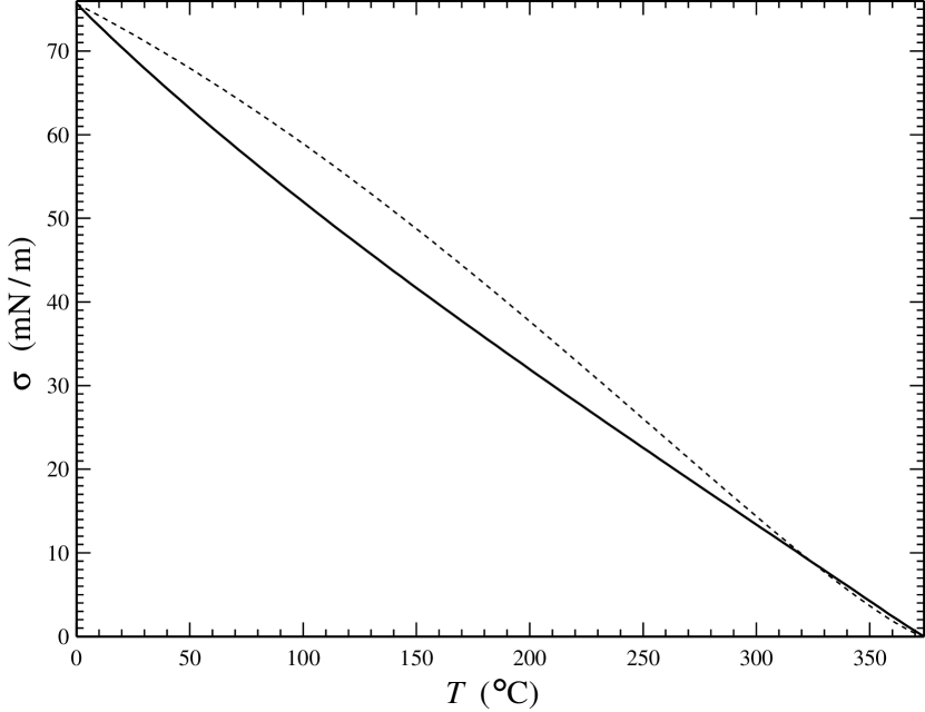
Figure 1: The surface tension $\sigma$ of the interface between liquid water and its vapor vs. the temperature $T$. The temperature varies from water’s triple-point value to its critical value. The solid curve shows the results computed through the DIM, the dotted curve shows the corresponding empiric results [23].

IV.3 Discussion: the width of a liquid–vapor interface

It is instructive to consider the boundary-value problem (36)-(39) in the small-temperature limit. Assuming the Enskog–Vlasov EoS (8) and omitting the term involving $T$, one can write (36) in the form

$$-2a\frac{\mathrm{d}\rho_{lv}}{\mathrm{d}z}=K\frac{\mathrm{d}^{2}\rho_{lv}}{\mathrm{d}z^{2}}.$$ (43)

At low $T$, the vapor density is negligible, whereas the liquid density is close to its triple-point density – so that the boundary conditions (37)-(38) become

$$\rho \rightarrow\rho_{tp}\qquad\text{as}\qquad z\rightarrow-\infty,$$ (44)

$$\rho \rightarrow 0\hskip 27.88358pt\text{as}\qquad z\rightarrow+\infty,$$ (45)

The solution of the boundary-value problem (43)-(45) is

$$\rho=\left\{\begin{tabular}[c]{ll}$\rho_{tp}$\vskip 6.0pt plus 2.0pt minus 2.0pt&if$\qquad z\leq-\frac{1}{2}W,$\\ $\tfrac{1}{2}\rho_{tp}\left(1-\sin\dfrac{\pi z}{W}\right)\qquad$\vskip 6.0pt plus 2.0pt minus 2.0pt&if$\qquad\left|z\right|<~{}\frac{1}{2}W,$\\ $0$&if$\qquad z\geq~{}~{}~{}\frac{1}{2}W,$\end{tabular}\ \right.$$

where

$$W=\pi\left(\frac{K}{2a}\right)^{1/2}$$ (46)

is, physically, the low-$T$ limit of the width of the interface. Expression (46) agrees qualitatively with the estimate of the interfacial thickness obtained in Refs. [24, 25]: if adapted for the Enskog–Vlasov EoS and $T=0$, the latter yields a result which is $\pi$ times smaller than (46).

Substituting estimates (42) for $K$ and (57) for $a$ into expression (46), one obtains

$$W\approx 2.40\times 10^{-10}\mathrm{m}.$$ (47)

It is also instructive to estimate the characteristic intermolecular distance $D$ for liquid water – at, say, the triple point:

$$D\approx n_{tp}^{-1/3}\approx 3.11\times 10^{-10}\mathrm{m},$$

where $n_{tp}$ is the triple-point number density.

Thus, for small $T$, the thickness of the liquid–vapor interface is comparable to the intermolecular distance. With increasing $T$, estimate (47) becomes invalid, as thermal motion of molecules erodes the interface, making it thicker. Finally, when $T$ approaches the critical point, the liquid–vapor interface becomes much thicker than $D$.

Note that the DIM is not the first hydrodynamic model to be used at scales comparable to $D$, where it is not formally applicable. The standard Navier-slip boundary condition – routinely used in almost all studies of contact lines – implies the same. The justification of using hydrodynamic models at small scales is as follows: even though they cannot accurately predict the microscopic characteristics of interfaces, the structure of those is still qualitatively correct – as is (sic!) their effect on the macroscopic flow. This appears to be true for the DIM, which predicts the correct macroscopic properties of fluids in equilibrium (the Maxwell construction), as well as their surface tension.

Note also that small interfacial thickness might hamper applications of the DIM with a realistic EoS to numerical modeling of contact lines. One should still be able to use it in conjunction with the numerical techniques recently developed for nucleation and collapse of vapor bubbles [26, 24, 27] and drops impacting on a solid surface [28].

V The contact angle vs. temperature

To define the contact angle, one needs to introduce the boundary-value problems describing solid–liquid and solid–vapor interfaces (the same way problem (36)-(38) describes liquid–vapor interfaces). To do so, introduce $\rho_{sl}(z)$ and $\rho_{sv}(z)$ satisfying

$$\frac{1}{\rho_{sl}}\frac{\mathrm{d}p(\rho_{sl},T)}{\mathrm{d}z}=K\frac{\mathrm{d}^{3}\rho_{sl}}{\mathrm{d}z^{3}},$$ (48)

$$\rho_{sl} =\rho_{0}\hskip 20.77039pt\text{at}\qquad z=0,$$ (49)

$$\rho_{sl} \rightarrow\rho_{l}\qquad\text{as}\qquad z\rightarrow+\infty,$$ (50)

and

$$\frac{1}{\rho_{sv}}\frac{\mathrm{d}p(\rho_{sv},T)}{\mathrm{d}z}=K\frac{\mathrm{d}^{3}\rho_{sv}}{\mathrm{d}z^{3}},$$ (51)

$$\rho_{sv} =\rho_{0}\hskip 22.76228pt\text{at}\qquad z=0,$$ (52)

$$\rho_{sv} \rightarrow\rho_{v}\qquad\text{as}\qquad z\rightarrow+\infty,$$ (53)

where $\rho_{l}$ and $\rho_{v}$ are determined by the Maxwell construction (39).

Next, let the solid surface coincide with the $\left(x,y\right)$ plane and the contact line, with the $y$ axis. This setting is described by the two-dimensional version of (35),

$$G-G_{0}=K\left(\frac{\partial^{2}\rho}{\partial x^{2}}+\frac{\partial^{2}\rho}{\partial z^{2}}\right),$$

and the following boundary conditions:

$$\rho=0\qquad\text{at}\qquad z=0,$$

$$\rho\rightarrow\rho_{sg}(z)\qquad\text{as}\qquad x\rightarrow-\infty,$$ (54)

$$\rho\rightarrow\rho_{sl}(z)+\rho_{lv}(z\cos\theta-x\sin\theta)\qquad\text{as}\qquad x\rightarrow+\infty,$$ (55)

where the contact angle $\theta$ is implied to be less than $90^{\circ}$ (i.e., the solid is hydrophilic). As shown in Ref. [3], one can find $\theta$ without solving the above boundary-value problem:

$$\left[{\displaystyle\int_{-\infty}^{\infty}}\left(\dfrac{\mathrm{d}\rho_{lv}}{\mathrm{d}z}\right)^{2}\mathrm{d}z\right]\cos\theta\\ ={\displaystyle\int_{0}^{\infty}}\left(\dfrac{\mathrm{d}\rho_{sv}}{\mathrm{d}z}\right)^{2}\mathrm{d}z-{\displaystyle\int_{0}^{\infty}}\left(\dfrac{\mathrm{d}\rho_{sl}}{\mathrm{d}z}\right)^{2}\mathrm{d}z.$$ (56)

If $\theta>90^{\circ}$ (hydrophobic solids), the boundary conditions (54)-(55) need to be slightly modified, but expression (56) remains exactly the same.

Thus, $\theta$ can be computed by integrating the boundary-value problems (48)-(50) and (51)-(53) numerically and substituting their solutions into expression (56). The solution of problem (36)-(38) is not needed, as it can be readily shown that

$${\displaystyle\int_{-\infty}^{\infty}}\left(\dfrac{\mathrm{d}\rho_{lv}}{\mathrm{d}z}\right)^{2}\mathrm{d}z={\displaystyle\int_{0}^{\infty}}\left(\dfrac{\mathrm{d}\rho_{sv}}{\mathrm{d}z}\right)^{2}\mathrm{d}z+{\displaystyle\int_{0}^{\infty}}\left(\dfrac{\mathrm{d}\rho_{sl}}{\mathrm{d}z}\right)^{2}\mathrm{d}z.$$

Unfortunately, there seems to be no measurements of the contact angle of a single-fluid interface, on a substrate with a sufficiently narrow hysteresis interval. Thus, instead of examining a specific water–substrate combination, $\theta$ was computed for the full range of $\rho_{0}$ – from zero to the triple-point density. The results are presented in Fig. 2.

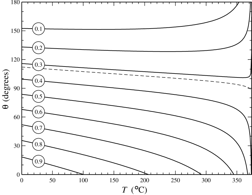
Figure 2: The static contact angle $\theta$ vs. the temperature $T$, for water. The curves are labelled with the corresponding values of $\rho_{0}/\rho_{tp}$ where $\rho_{tp}$ is the triple-point density of liquid water. The separatrix (dashed line) corresponds to $\rho_{0}$ coinciding with the critical density.

Evidently, for all $\rho_{0}$ except a certain separatrix value, a temperature exists such that the contact angle either becomes  equal to $180^{\circ}$ (perfect hydrophobicity) or $0^{\circ}$ (perfect hydrophilicity). The former occurs if $\rho_{0}$ matches the saturated-vapor density $\rho_{v}(T)$ and the latter, if $\rho_{0}$ matches the liquid density $\rho_{l}(T)$. It is also clear that the separatrix corresponds to $\rho_{0}$ equal to the critical density.

VI Summary and concluding remarks

Thus, the following results have been obtained:

1. It has been shown that the boundary condition prescribing the density of a fluid at a solid wall can be derived without assuming that the solid–fluid interaction is short-ranged by comparison with the fluid–fluid one (as conjectured in Ref. [3]). Thus, this boundary condition is based on the same physics as the DIM itself.

2. A parameter region has been identified [$\beta\ll 1$ with $\beta$ determined by (23)], where interfacial flows without external heating are almost isothermal. This region does not include water, where the heat production due to viscosity and compressibility of vapor near the interface is too strong.
         It is worth mentioning that interfaces are likely to be isothermal in fluids with high viscosity, such as glycerol or ethylene glycol. This claim is supported by the estimates carried out in Ref. [14] using the van der Waals EoS; even though it is much less accurate than the Enskog–Vlasov EoS used in the present work, it still works qualitatively correct for water. Physically, high viscosity slows the flow down and, thus, reduces the heat production.

3. The DIM was coupled with a realistic EoS of water and used to compute the surface tension $\sigma$ of a liquid/vapor interface as a function of the temperature $T$ (Sect. IV, Fig. 1). The theoretical results agree well with the empiric dependence $\sigma(T)$.

4. The static contact angle $\theta$ of a liquid–vapor interface has been computed as a function of $T$ for water (Sect. V, Fig. 2). The results obtained predict that, with increasing $T$, any substrate would become either perfectly hydrophobic ($\theta=180^{\circ}$) or perfectly hydrophilic ($\theta=0^{\circ}$).

Admittedly, (the most counter-intuitive) conclusion 4 has not been verified experimentally.

To do so in the future, one needs to experiment with a single-fluid interface and a chemically-cleaned or lubricant-impregnated substrate. The former requirement can be relaxed if the present results are extended to a mixture of fluids (e.g., water plus nitrogen). The latter requirement is crucial, however, as, for usual substrates, $\theta$ does not assume a reasonably well-defined value, but one from an often-wide hysteresis interval.

Still, there is qualitative evidence that the effects of induced hydrophobicity and hydrophilicity do occur in the real world.

It can be argued that states with $\theta=180^{\circ}$ or $\theta=0^{\circ}$ can be created through any parameter variation, not only that of the temperature. To do so, this variation should change either $\rho_{0}$ or the densities of the phases – until the former coincides with one of the latter: perfect hydrophobicity and hydrophilicity correspond to $\rho_{0}=\rho_{v}$ and $\rho_{0}=\rho_{l}$, respectively. This argument could explain the observed behavior of droplets under variable electric field [29].

Finally, note that a case has been made [30, 31] for switching from the simplified differential representation for the van der Waals force (used in this paper and all applications) to the full integral expression (9). It is not clear at this stage how this would effect our results.

Appendix A The Enskog–Vlasov equation of state

When applying the DIM to a specific fluid, one needs an EoS describing this fluid’s thermodynamic properties with a reasonable accuracy. In this work, the Enskog–Vlasov (EV) model will be used, where the internal energy and entropy per unit mass are given by Eqs. (7), and the EoS, by (8). Note that Eqs. (7)-(8) are invariant with respect to a simultaneous change

$$b\rightarrow\operatorname{const}\times b,\qquad\Theta(\xi)\rightarrow\Theta(\operatorname{const}^{-1}\times\xi).$$

Thus, to remove the ambiguity when choosing $b$, the restriction

$$\left[\frac{\mathrm{d}\Theta(\xi)}{\mathrm{d}\xi}\right]_{\xi=0}=\frac{2\pi}{3}$$

is traditionally imposed in the EV theory.

Before using EoS (8), one needs to calibrate it, i.e., specify $a$, $b$, and $\Theta(\xi)$, such that the fluid under consideration is described as accurately as possible. As for the specific heat capacity, it will be assigned the ideal-fluid value: for water, this amounts to

$$c_{V}=3R.$$

To fix $a$, observe that, as follows from (7),

$$\Delta e=c_{V}T-e$$

depends linearly on $\rho$. Thus, $a$ can be determined by fitting a linear function to the empiric dependence $\Delta e$ vs. $\rho$. Using the data from Ref. [32], one can estimate

$$a=2112~{}\mathrm{m}^{5}\mathrm{s}^{-2}\mathrm{kg}^{-1}.$$ (57)

(For simplicity, this estimate was obtained using only the data for the critical pressure $p=220.64~{}\mathrm{bar}$ and the temperature range $273.16~{}\mathrm{K}$ to $800.16~{}\mathrm{K}$.) The accuracy of representation (7) of the free energy can be assessed from Fig. 3 which shows the dependence $\Delta e$ vs. $\rho$ for three different isobars (including the critical one), together with the linear fit resulting estimate (57).

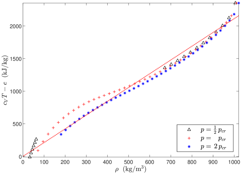
Figure 3: The non-ideal component of the internal energy vs. density. The non-connected symbols show the empiric data from Ref. [32] presented in isobaric form, for the values of the pressure $p$ (relative to the critical pressure $p_{cr}$) stated in the legend. The dotted line shows the linear fit of the critical isobar.

The parameter $b$, in turn, can be simply equated to the reciprocal of the triple-point density [17, 18] – hence, for water,

$$b=1.0002\times 10^{-3}\mathrm{m}^{3}\mathrm{kg}^{-1}.$$ (58)

Finally, let

$$\Theta(\xi)=\frac{2\pi}{3}\xi+\sum_{i=2}^{5}c_{i}\xi^{i},$$ (59)

with the coefficients $c_{i}$ being such that the equation of state (8), (57)-(59) describes correctly the fluid’s density and temperature at the triple and critical points, as well as the critical pressure (for more details, see Ref. [18]). In application to water, this yields

$$c_{2} =\hskip 12.80365pt4.649,\qquad c_{3}=1.642,$$ (60)

$$c_{4} =-10.108,\qquad c_{5}=7.973.$$ (61)

The accuracy of the EV model calibrated this way can be assessed from Figs. 4-5, which compare predictions of (8), (57)-(61) to the corresponding empiric results [32].

Figure 4: The parameters of liquid water and vapor in equilibrium: the empiric data from Ref. [32] (dotted line) and the results obtained through the EV model (solid line). (a) The densities of the saturated vapor and liquid (the upper and lower parts of the curves, respectively) vs. $T$. (b) The pressure of the saturated vapor vs. $T$.

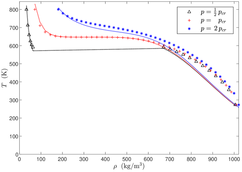
Figure 5: The equation of state for water: the empiric data [32] (non-connected symbols) and the results obtained through the EV model (dotted curves).

One can see, that the Enskog–Vlasov EoS is reasonably accurate and can be safely used in studies of flows with phase transitions.

Appendix B An example of solution of Eq. (28)

The solution of the inner-problem equation (28) will be illustrated by the simplest particular case of $\Psi$ and $U$, such that the former is approximated by a piece-wise-constant function

$$\Psi(\hat{z})=\left\{\begin{tabular}[c]{ll}$0\vskip 3.0pt plus 1.0pt minus 1.0pt$&if$\hskip 8.5359pt\hat{z}\in\left(-\infty,-2H\right),$\\ $-1\hskip 5.69046pt\vskip 3.0pt plus 1.0pt minus 1.0pt$&if$\hskip 8.5359pt\hat{z}\in\left[-2H,-H\right),$\\ $2\vskip 3.0pt plus 1.0pt minus 1.0pt$&if$\hskip 8.5359pt\hat{z}\in\left[-H,H\right],$\\ $-1\vskip 3.0pt plus 1.0pt minus 1.0pt$&if$\hskip 8.5359pt\hat{z}\in\left(H,2H\right],$\\ $0$&if$\hskip 8.5359pt\hat{z}\in\left(2H,\infty\right),$\end{tabular}\ \right.$$ (62)

and the latter is approximated by a piece-wise-linear function,

$$U(\hat{z})=\left\{\begin{tabular}[c]{ll}$U_{0}\hat{z}-\left(U_{0}+U_{1}\right)\Delta\hskip 5.69046pt\vskip 3.0pt plus 1.0pt minus 1.0pt$&if$\hskip 8.5359pt\hat{z}\in\left[0,H\right],$\\ $U_{1}\left(\hat{z}-2\Delta\right)\vskip 3.0pt plus 1.0pt minus 1.0pt$&if$\hskip 8.5359pt\hat{z}\in\left(H,2H\right],$\\ $0$&if$\hskip 8.5359pt\hat{z}\in\left(2H,\infty\right),$\end{tabular}\ \right.$$ (63)

where $\Delta$, $U_{0}$, and $U_{1}$ are constants. As required, the above $\Psi(\hat{z})$ satisfies restrictions (30).

Substituting (62)-(63) into Eq. (28), omitting hats, and introducing

$$\rho_{n}(z)=\rho(z+n\Delta)\qquad\text{if}\qquad z\in\left(0,\Delta\right],$$

one obtains

$$2\rho_{1}-\rho_{2}+U_{0} =0,$$

$$2\left(\rho_{2}-\rho_{0}\right)-\rho_{3}+U_{1} =0,$$

$$2\left(\rho_{n-1}-\rho_{n-3}\right)-\rho_{n}+\rho_{n-4} =0\qquad\text{for}\qquad n\geq 4.$$

One can use these (recursive) equations to calculate several first terms – then guess the general formula relating $\rho_{n}$ to $\rho_{0}$ and $\rho_{1}$ – then verify this formula by substitution – and thus obtain

$$\rho_{n}=\frac{n^{2}}{4}\left(\rho_{1}-\rho_{0}+U_{0}+U_{1}\right)\\ +\frac{n}{2}\left(\rho_{1}-U_{1}\right)+\rho_{0}\qquad\text{for even }n\geq 0,$$ (64)

$$\rho_{n}=\frac{n^{2}}{4}\left(\rho_{1}-\rho_{0}+U_{0}+U_{1}\right)+\frac{n}{2}\left(\rho_{1}-U_{1}\right)\\ +\frac{1}{4}\left(\rho_{1}+\rho_{0}-U_{0}+U_{1}\right)\qquad\text{for odd }n\geq 1.$$ (65)

Observe that the quadratic dependence of $\rho$ on $n$ is in line with that of $\rho$ on $z$ in asymptotic (31).

As shown in the main body of the paper, the inner solution matches the outer one only if the former does not grow as $z\rightarrow\infty$. Thus, the growing terms in expressions (64)-(65) should be eliminated, which implies $\rho_{0}=U_{0}$, $\rho_{1}=-U_{1}$, and

$$\rho_{n}=U_{0}+2U_{1}\qquad$$

This solution is bounded, but it oscillates, so still does not have the desired (uniform) asymptotics as $z\rightarrow\infty$. The only way to eliminate the oscillations is to require that $U_{0}=-U_{1}$ – in which case $\rho_{n}=U$ for all $n$ – hence, $\rho(z)=U_{1}$ for all $z$, and

$$\rho_{0}=U_{1}.$$

The fact that the near-wall region can generate short-scale oscillations and potentially ‘send’ them (through the matching conditions) into the whole domain is interesting from the mathematical viewpoint. Physically, however, such cases should be avoided, just like one of them has been avoided in the above example.

In general, one can show that the large-$z$ asymptotics of the solution of Eq. (28) has a periodic component only if the Fourier transform of $\Psi(z)$,

$$\hat{\chi}(k)=\int_{0}^{\infty}\Psi(z)\cos kz\,\mathrm{d}z,$$

vanishes at some $k$. One can also show that the periodic component disappears if the Fourier transform of $U(z)$ vanishes at the same value(s) of $k$ (which is what happens in the above example when the condition $U_{0}=-U_{1}$ was applied).

References

- Gouin [1987] H. Gouin, Utilization of the Second Gradient Theory in continuum mechanics to study the motion and thermodynamics of liquid–vapor interfaces, in Physicochemical Hydrodynamics, NATO ASI Series, Vol. 174, edited by M. G. Velarde (Springer US, 1987) pp. 667–682.
- Anderson et al. [1998] D. M. Anderson, G. B. McFadden, and A. A. Wheeler, Diffuse-interface methods in fluid mechanics, Annu. Rev. Fluid Mech. 30, 139 (1998).
- Pismen and Pomeau [2000] L. M. Pismen and Y. Pomeau, Disjoining potential and spreading of thin liquid layers in the diffuse-interface model coupled to hydrodynamics, Phys. Rev. E 62, 2480 (2000).
- Jacqmin [2000] D. Jacqmin, Contact-line dynamics of a diffuse fluid interface, J. Fluid Mech. 402, 57 (2000).
- Korteweg [1901] D. J. Korteweg, Sur la forme que prennent les équations du mouvement des fluides si l’on tient compte des forces capillaires causées par des variations de densité considérables mais continues et sur la théorie de la capillarité dans l’hypothése d’une variation continue de la densité, Arch. Néerl. Sci. Ex. Nat. Ser. 2 6, 1 (1901).
- Seppecher [1996] P. Seppecher, Moving contact lines in the Cahn-Hilliard theory, Int. J. Eng. Sci. 34, 977 (1996).
- Ding and Spelt [2007] H. Ding and P. D. M. Spelt, Wetting condition in diffuse interface simulations of contact line motion, Phys. Rev. E 75, 046708 (2007).
- Yue and Feng [2011] P. Yue and J. J. Feng, Can diffuse-interface models quantitatively describe moving contact lines?, Eur. Phys. J. Spec. Top. 197, 37 (2011).
- Kusumaatmaja et al. [2016] H. Kusumaatmaja, E. J. Hemingway, and S. M. Fielding, Moving contact line dynamics: from diuse to sharp interfaces, J. Fluid Mech. 788, 209 (2016).
- Fakhari and Bolster [2017] A. Fakhari and D. Bolster, Diffuse interface modeling of three-phase contact line dynamics on curved boundaries: A lattice Boltzmann model for large density and viscosity ratios, J. Comput. Phys. 334, 620 (2017).
- Borcia et al. [2019] R. Borcia, I. D. Borcia, M. Bestehorn, O. Varlamova, K. Hoefner, and J. Reif, Drop behavior influenced by the correlation length on noisy surfaces, Langmuir 35, 928 (2019).
- Caupin [2005] F. Caupin, Liquid-vapor interface, cavitation, and the phase diagram of water, Phys. Rev. E 71, 051605 (2005).
- Onuki [2007] A. Onuki, Dynamic van der Waals theory, Phys. Rev. E 75, 036304 (2007).
- Benilov [2020] E. S. Benilov, Asymptotic reductions of the diffuse-interface model, with applications to contact lines in fluids, arXiv 1907.04434 (2020), http://arxiv.org/abs/1907.04434v3 .
- de Sobrino [1967] L. de Sobrino, On the kinetic theory of a van der waals gas, Can. J. Phys. 45, 363 (1967).
- Grmela [1971] M. Grmela, Kinetic equation approach to phase transitions, J. Stat. Phys. 3, 347 (1971).
- Benilov and Benilov [2018] E. S. Benilov and M. S. Benilov, Energy conservation and theorem for the Enskog-Vlasov equation, Phys. Rev. E 97, 062115 (2018).
- Benilov and Benilov [2019] E. S. Benilov and M. S. Benilov, Peculiar property of noble gases and its explanation through the Enskog-Vlasov model, Phys. Rev. E 99, 012144 (2019).
- Ferziger and Kaper [1972] J. H. Ferziger and H. G. Kaper, Mathematical theory of transport processes in gases (Elsevier, New York, 1972).
- Haynes et al. [2017] W. M. Haynes, D. R. Lide, and T. J. Bruno, CRC handbook of chemistry and physics (Taylor & Francis, Boca Raton, 2017).
- Mauri [2013] R. Mauri, Non-equilibrium thermodynamics in multiphase flows (Springer, Dordrecht, 2013).
- Note [1] If, for a fluid under consideration, the surface tension of the liquid–vapor interface has never been measured, but has been computed through (presumably highly accurate) molecular and Monte Carlo simulations, one can benchmark the prediction of Eq. (40) against the results of the latter (as done in Ref. [27]).
- Wagner and Kretzschmar [2008] W. Wagner and H.-J. Kretzschmar, International steam tables (Springer, Berlin Heidelberg, 2008) p. 388.
- Magaletti et al. [2016] F. Magaletti, M. Gallo, L. Marino, and C. M. Casciola, Shock-induced collapse of a vapor nanobubble near solid boundaries, Int. J. Multiphase Flow 84, 34 (2016).
- Gallo et al. [2020] M. Gallo, F. Magaletti, D. Cocco, and C. M. Casciola, Nucleation and growth dynamics of vapour bubbles, J. Fluid Mech. 883, A14 (2020).
- Magaletti et al. [2015] F. Magaletti, L. Marino, and C. M. Casciola, Shock wave formation in the collapse of a vapor nanobubble, Phys. Rev. Lett. 114, 064501 (2015).
- Gallo et al. [2018] M. Gallo, F. Magaletti, and C. M. Casciola, Thermally activated vapor bubble nucleation: The landau-lifshitz–van der waals approach, Phys. Rev. Fluids 3, 053604 (2018).
- Gelissen et al. [2020] E. J. Gelissen, C. W. M. van der Geld, M. W. Baltussen, and J. G. M. Kuerten, Modeling of droplet impact on a heated solid surface with a diffuse interface model, Int. J. Multiphase Flow 123, 103173 (2020).
- Brabcova et al. [2017] Z. Brabcova, G. McHale, G. G. Wells, C. V. Brown, and M. I. Newton, Electric field induced reversible spreading of droplets into films on lubricant impregnated surfaces, Appl. Phys. Lett. 110, 121603 (2017).
- Pismen [2001] L. M. Pismen, Nonlocal diffuse interface theory of thin films and the moving contact line, Phys. Rev. E 64, 021603 (2001).
- Yochelis and Pismen [2006] A. Yochelis and L. M. Pismen, Thin films of van der Waals fluid: From interface interactions to wetting transitions, Colloids Surf., A 274, 170 (2006).
- Linstrom and Mallard [1997] P. J. Linstrom and W. G. Mallard, NIST chemistry webbook, NIST standard reference database number 69 (1997).