Rethinking Depthwise Separable Convolutions:
How Intra-Kernel Correlations Lead to Improved MobileNets

Abstract

We introduce blueprint separable convolutions (BSConv) as highly efficient building blocks for CNNs. They are motivated by quantitative analyses of kernel properties from trained models, which show the dominance of correlations along the depth axis. Based on our findings, we formulate a theoretical foundation from which we derive efficient implementations using only standard layers. Moreover, our approach provides a thorough theoretical derivation, interpretation, and justification for the application of depthwise separable convolutions (DSCs) in general, which have become the basis of many modern network architectures. Ultimately, we reveal that DSC-based architectures such as MobileNets implicitly rely on cross-kernel correlations, while our BSConv formulation is based on intra-kernel correlations and thus allows for a more efficient separation of regular convolutions. Extensive experiments on large-scale and fine-grained classification datasets show that BSConvs clearly and consistently improve MobileNets and other DSC-based architectures without introducing any further complexity. For fine-grained datasets, we achieve an improvement of up to 13.7 percentage points. In addition, if used as drop-in replacement for standard architectures such as ResNets, BSConv variants also outperform their vanilla counterparts by up to 9.5 percentage points on ImageNet. Code and models are available under https://github.com/zeiss-microscopy/BSConv.

1 Introduction

Convolutional neural networks (CNNs) [27, 26] have become the basis of practically all state-of-the-art approaches for image classification, object detection [5], semantic segmentation [30], and many other applications. In the past, improvements of CNNs were mainly driven by increasing the model capacity, while at the same time ensuring a proper training behavior [20, 13, 14]. Recently, this has led to the development of models with half a billion parameters [18]. In practical applications, however, the computational capacity is often limited, especially in mobile and automotive contexts. This fact has led to another important research direction which focuses on improving model efficiency. The most prominent approaches are based on depthwise separable convolutions (DSCs) [37, 16]—building blocks which are motivated by exploiting redundancies of filter weights.

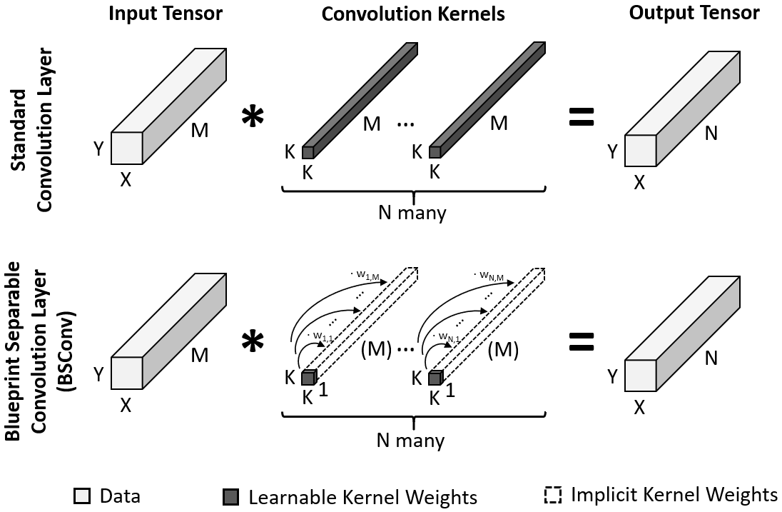
Figure 1: We introduce blueprint separable convolutions (BSConv) as highly efficient building block for CNNs. BSConv exploits correlations of CNN kernels along their depth axis. In consequence, BSConv represents each filter kernel using one 2d blueprint kernel which is distributed along the depth axis using a weight vector.

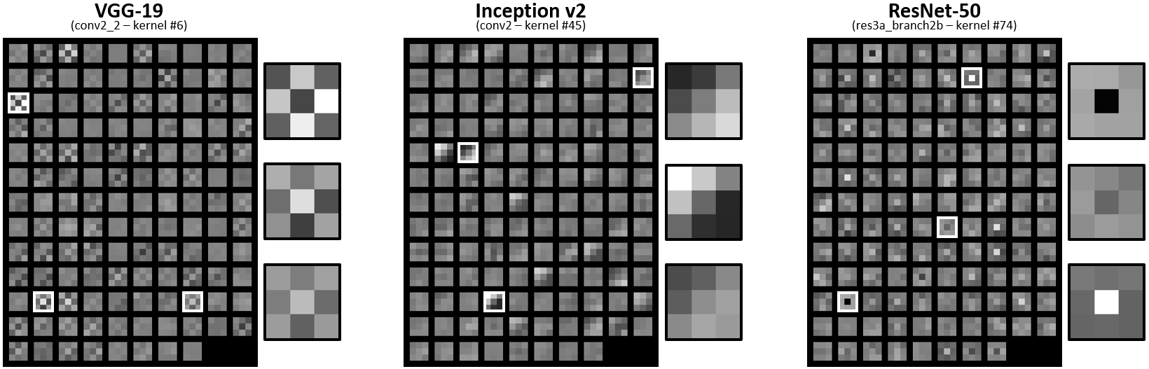
Figure 2: Exemplary filter weights of a vanilla VGG-19, Inception v2, and ResNet-50 CNN trained on ImageNet. For each of the three CNN architectures, one filter kernel of size $M\times K\times K=128\times 3\times 3$ is visualized, split into 128 images. The weights of each filter kernel are highly correlated along the depth axis. Concretely, most slices show the same filter-specific $3\times 3$ ‘blueprint’, only scaled by different factors (including negative factors which cause ‘inverted’ versions of the blueprint). While only three slices are highlighted for each kernel, the correlation is visible for far more slices (52/128 for the ResNet-50 example). This observation is the motivation for our proposal of blueprint separable convolutions (BSConv), which inherently represent a filter kernel of size $M\times K\times K$ using one blueprint kernel of size $K\times K$ and a set of $M$ multiplicative factors used to distribute the blueprint across the depth axis.

Based on quantitative and qualitative analyses of trained CNNs, in Section 3 we propose blueprint separable convolutions (BSConv), which follow this path of research. The main idea of BSConv is to exploit that kernels of CNNs usually show high redundancies along their depth axis (i.e., intra-kernel correlations). Thus, BSConv represents each filter kernel using one 2d blueprint which is distributed along the depth axis using a weight vector (see Figure 1).

Although DSCs are also motivated by intra-kernel correlations [37], in Section 4 we show that their derived order of operations contradicts this assumption and is reversed compared to our BSConv solution. In fact, the DSC result is equivalent to assuming redundancies between kernels (i.e., cross-kernel correlations, see Figure 5), which was shown to be less effective when separating convolutions [7]. In addition, a natural extension of BSConv leads to an interpretation and justification for DSCs with linear bottlenecks [35], which are extensively used in many recent models [15, 40, 41]. Our solution, however, directly implies the use of an additional regularization loss to improve the subspace transform implicitly performed by these bottlenecks.

In Section 5, we thoroughly demonstrate that BSConv consistently outperforms DSC-based architectures such as MobileNets on a wide variety of large-scale and fine-grained datasets at the same parameter and time complexity. Furthermore, BSConv can be used as drop-in replacement for standard convolution layers and can be applied to other architectures as well, leading to performance gains while drastically increasing model efficiency.

2 Related Work

Numerous approaches exist to improve the efficiency of CNNs. One example is model pruning, where filters and/or connections are removed from CNNs during or after model training [10, 28, 11, 29]. Closely related and often combined are quantization [33, 47, 19] and compression techniques [6, 9, 8] to accelerate model inference.

Another relevant research area is efficiency-driven CNN architecture search. It can be performed manually [12] or automatically, e.g. via genetic algorithms [43] or via reinforcement learning in the form of neural architecture search [48, 1]. The latter is the basis for the most recent advances in building efficient models such as MnasNet [40], MobileNetV3 [15], and EfficientNet [41].

Building blocks typically consist of activation, normalization, and convolution operations, where the latter bear the greatest potential for efficiency optimizations. Redundancies in convolution weights of trained CNNs are analyzed in [3, 37, 36, 7]. Approaches to reduce these redundancies are for instance low-rank approximations of the filter kernels [4, 21, 22] and the usage of grouped convolutions [46, 31, 44]. In [37], DSCs are introduced, which form the basis for practically all recent efficient network architectures. Their direct application can for instance be found in MobileNetV1 [16], factorized CNNs [42], and Xception [2]. An extension of DSCs are inverted residual bottlenecks which are introduced in MobileNetV2 [35]. They are used in state-of-the-art efficient architectures, including MnasNet [40], MobileNetV3 [15], and EfficientNet [41].

3 Blueprint Separable Convolutions (BSConv)

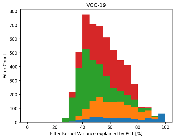
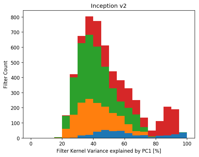
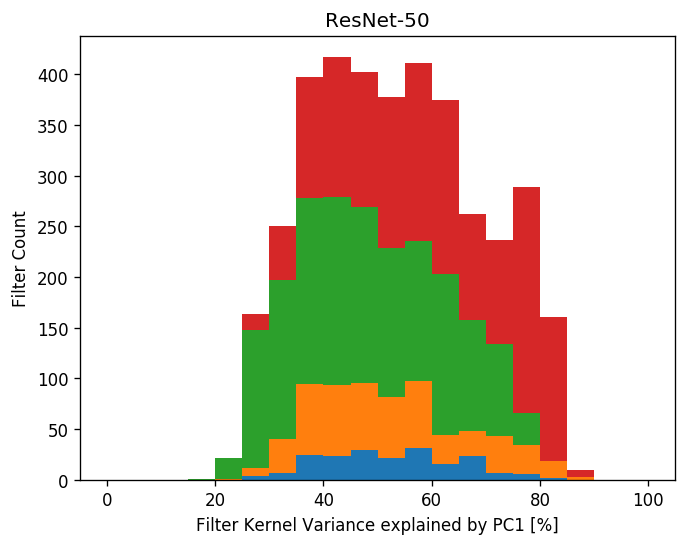
Figure 3: Histogram of the variance along the depth axis of filter kernels which can be explained using only one principal component per filter. The filters are grouped by convolution stages (stage 1: blue, stage 2: orange, stage 3: green, stage 4: red). These quantitative results show that a large portion of CNN filters can potentially be represented using our BSConv formulation. This figure is best viewed in color.

In standard CNNs, each convolution layer transforms an input tensor $U$ of size $M\times Y\times X$ into an output tensor $V$ of size $N\times Y\times X$ by applying convolution kernels $F^{(1)},\dots,F^{(N)}$, each of size $M\times K\times K$ such that

$$V_{n,:,:}=U*F^{(n)}$$ (1)

with $n\in\left\{1,\dots,N\right\}$ (see Figure 1, top row). The entries (or ‘weights’) of these $N$ kernels are optimized during the training stage of CNNs via backpropagation and may take arbitrary values. However, in the following we show that in practice these weights often converge towards a state in which they show a substantial amount of correlation. We analyze these correlations qualitatively and quantitatively, and then derive a new, parameter- and time-efficient version of convolution layers for CNNs based on our findings.

3.1 Intra-Kernel Correlations in Standard CNNs

In this paper we focus on intra-kernel correlations and their potential for the design of parameter- and time-efficient CNNs. We start with a qualitative analysis of intra-kernel correlations by visualizing filters of trained CNNs. Figure 2 shows exemplary filter kernels for three established CNN architectures trained on the ImageNet dataset—namely VGG-19 [38], Inception v2 [20], and ResNet-50 [13, 14]. From these visualizations, it can be seen that intra-kernel correlations exist along the depth axis. Concretely, it often seems that for a filter $F^{(n)}$, its slices $F^{(n)}_{1,:,:},\dots,F^{(n)}_{M,:,:}$ show the same filter-specific $K\times K$ ‘blueprint’, only scaled by different factors (including negative factors which cause ‘inverted’ versions of the blueprint).

While Figure 2 shows only a small subset of filter kernels, the described property of filter slices being based on a ‘blueprint’ are by no means an exception. According to our observations, it occurs consistently across different CNN architectures, training settings, and datasets. To systematically quantify to which extent filter kernels show this behavior, we analyze several trained CNNs in the following way: For each individual filter of the CNN, we (i) split the $M\times K\times K$ kernel into $M$ samples of size $K\times K$, (ii) perform principal component analysis (PCA) on the set of $M$ samples, and (iii) determine the variance of the filter kernel which is explained by the first principal component (PC1). Using this approach, we can quantify how well each filter is representable by a $K\times K$ filter-specific blueprint (which in this case corresponds to PC1) and $M$ factors (which in this case are the ‘scores’ obtained via PCA). We aggregate these individual values into histograms, which are shown in Figure 3 for the same vanilla CNNs used in Figure 2. It can be seen that on average, about 50% of each filter kernel’s variance can be explained using this simple model, suggesting a large potential for efficiency improvements.

3.2 From Correlations to BSConv

The analysis in Section 3.1 suggests that for trained vanilla CNNs, each $M\times K\times K$ filter can be approximated using a $K\times K$ blueprint and $M$ factors which ‘distribute’ the blueprint along the depth dimension. Even though it is by no means enforced during training, this approximation explains a large portion of the observed variance. This finding is the motivation for the introduction of blueprint separable convolutions (BSConv). They are defined in such a way that above approximation turns into an integral property of the filters of CNNs. Concretely, we define each filter kernel $F^{(n)}$ to be represented using a blueprint $B^{(n)}$ and the weights $w_{n,1},\dots,w_{n,M}\in\mathbb{R}$ via

$$F^{(n)}_{m,:,:}=w_{n,m}\cdot B^{(n)},$$ (2)

with $m\in\left\{1,\dots,M\right\}$ and $n\in\left\{1,\dots,N\right\}$ (see Figure 1, bottom row). While this definition poses a hard constraint on the filter kernels, in Section 5 we experimentally show that CNNs trained with BSConv can reach the same or even better quality in comparison to their vanilla counterparts. However, in contrast to standard convolution layers which have $M\cdot N\cdot K^{2}$ free parameters (see Figure 1), the BSConv variant only has $N\cdot K^{2}$ parameters for the blueprints, and $M\cdot N$ parameters for the weights. As is discussed below, the latter can be reduced even further.

3.3 Variants and Implementations

A BSConv module consists of $N$ filters, each having one blueprint and $M$ weights. All $M\cdot N$ weights can be combined into the matrix $W=(w_{n,m})$. Depending on how $W$ is learned in the training step, different BSConv variants can be derived. In the following, two variants are described.

3.3.1 Unconstrained BSConv (BSConv-U)

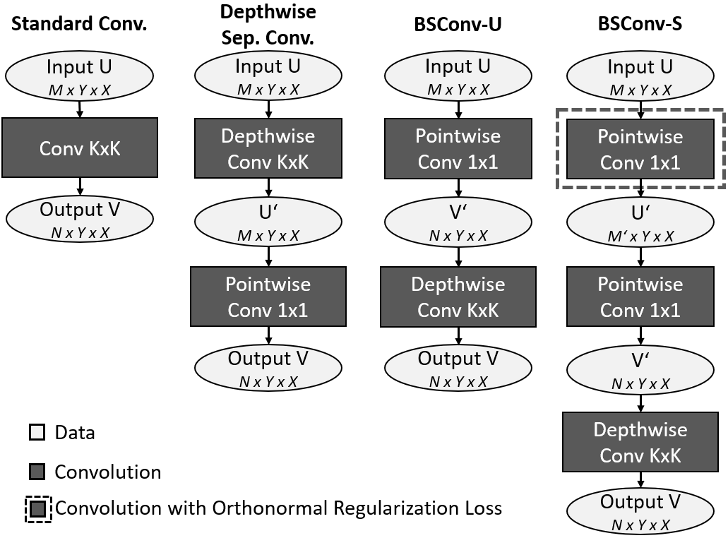
Figure 4: Computational graphs for the efficient implementation of the different BSConv variants (see Sections 3.3.1 and 3.3.2).

In the most general case, the weights $W$ can vary without any constraints and are learned directly via backpropagation, just like the entries of the blueprint filter kernels.

As shown in Figure 1, a naive implementation can be achieved by constructing a full kernel from each blueprint and performing a regular convolution afterwards. However, to derive a much more efficient implementation for CNNs, we rewrite Equation 1 in the following way: Firstly, because the input data tensor $U$ and the filter kernels $F^{(1)},\dots,F^{(N)}$ have the same size $M$ along their depth dimension, we can split each 3d convolution into a sum of $M$ 2d convolutions, yielding

$$V_{n,:,:}=U*F^{(n)}=\sum_{m=1}^{M}\left(U_{m,:,:}*F^{(n)}_{m,:,:}\right).$$ (3)

Secondly, we can replace each filter with its BSConv representation as given in Equation 2, and obtain

$$V_{n,:,:}=\sum_{m=1}^{M}\left(U_{m,:,:}*\left(w_{n,m}\cdot B^{(n)}\right)\right).$$ (4)

Because (i) each filter blueprint $B^{(n)}$ is independent of the input channel $m$, and (ii) $w_{n,m}$ is a scalar, we can rearrange above equation into

$$V_{n,:,:}=\underbrace{\Big{(}\sum_{m=1}^{M}U_{m,:,:}\cdot w_{n,m}\Big{)}}_{V_{n,:,:}^{\prime}}*B^{(n)}.$$ (5)

If we further rearrange $w_{n,1},\dots,w_{n,M}$ into a $M\times 1\times 1$ array $\tilde{w}_{n}$, the sum can be replaced by a convolution, giving

$$V_{n,:,:}^{\prime} =U*\tilde{w}_{n}$$ (6)

$$V_{n,:,:} =V_{n,:,:}^{\prime}*B^{(n)}.$$ (7)

For a concrete implementation, these Equations 6 and 7 can directly be translated into two tensor operations: (i) a $1\times 1$ pointwise convolution with the kernels $\tilde{w}_{1},\dots,\tilde{w}_{N}$, which is performed on the input data tensor $U$, and (ii) a $K\times K$ depthwise convolution [16, 20] with kernels $B^{(1)},\dots,B^{(N)}$, which is applied to the result of the first step. A flowchart visualization of these steps is given in Figure 4.

3.3.2 Subspace BSConv (BSConv-S)

For CNNs trained with BSConv-U convolution layers, the free parameters to be estimated are the $N$ blueprint kernel matrices and the weight matrix $W=(w_{n,m})$ of size $N\times M$. When analyzing the structure of the weight matrices $W$ of such CNNs, we observe that the rows of $W$ are often highly correlated. This fact indicates the potential for a further regularization and parameter reduction.

Concretely, we perform a low-rank approximation of $W$ by factorizing it into the $N\times M^{\prime}$ matrix $W^{A}=(w^{A}_{n,m^{\prime}})$ and the $M^{\prime}\times M$ matrix $W^{B}=(w^{B}_{m^{\prime},m})$ as

$$W=W^{A}\cdot W^{B},$$ (8)

with $M^{\prime}=\lceil p\cdot M\rceil$, while $p\in(0.0,1.0)$ specifies the size of the subspace $M^{\prime}$ in relation to the size $M$ of the original space. The matrix $W^{B}$ can be thought of as set of $M^{\prime}$ basis vectors, while $W^{A}$ is the subspace version of $W$. Instead of $N\cdot M$ weights as for the case of BSConv-U, this method reduces the parameter count to $N\cdot M^{\prime}+M^{\prime}\cdot M$, as only $W^{A}$ and $W^{B}$ have to be learned via backpropagation.

To minimize redundancies in the low-rank subspace, we want the basis defined by $W^{B}$ to be orthonormal. This can be achieved via the regularization loss

$$L_{\text{ortho}}=\big{\lVert}W^{B}{W^{B}}^{\text{T}}-I\big{\rVert}_{\text{F}},$$ (9)

where $I$ is the identity matrix and $\lVert\cdot\rVert_{\text{F}}$ the Frobenius norm of a matrix. The regularization loss is added to the classification loss $L_{\text{class}}$ with the weighting factor $\alpha$, resulting in the joint loss $L=L_{\text{class}}+\alpha L_{\text{ortho}}$.

To derive an efficient implementation of BSConv-S, we can substitute $w_{n,m}=\sum_{m^{\prime}=1}^{M^{\prime}}w^{A}_{n,m^{\prime}}\cdot w^{B}_{m^{\prime},m}$ in Equation 5, yielding

$$V_{n,:,:}=\Bigg{(}\sum_{m=1}^{M}U_{m,:,:}\cdot\Big{(}\sum_{m^{\prime}=1}^{M^{\prime}}w^{A}_{n,m^{\prime}}\cdot w^{B}_{m^{\prime},m}\Big{)}\Bigg{)}*B^{(n)}.$$ (10)

Using the same arguments as in Section 3.3.1, we can rearrange this equation into

$$V_{n,:,:}=\overbrace{\Bigg{(}\sum_{m^{\prime}=1}^{M^{\prime}}\underbrace{\Big{(}\sum_{m=1}^{M}U_{m,:,:}\cdot w^{B}_{m^{\prime},m}\Big{)}}_{U^{\prime}_{m^{\prime},:,:}}\cdot w^{A}_{n,m^{\prime}}\Bigg{)}}^{V^{\prime}_{n,:,:}}*B^{(n)}.$$ (11)

By rearranging the weights $w^{B}_{m^{\prime},1},\dots,w^{B}_{m^{\prime},M}$ into the $M\times 1\times 1$ array $\tilde{w}^{B}_{m^{\prime}}$ and the weights $w^{A}_{n,1},\dots,w^{A}_{n,M^{\prime}}$ into the $M^{\prime}\times 1\times 1$ array $\tilde{w}^{A}_{n}$, the sums can be replaced by convolutions in the same way as in Section 3.3.1, and we obtain

$$U^{\prime}_{m^{\prime},:,:} =U*\tilde{w}^{B}_{m^{\prime}}$$ (12)

$$V^{\prime}_{n,:,:} =U^{\prime}*\tilde{w}^{A}_{n}$$ (13)

$$V_{n,:,:} =V^{\prime}_{n,:,:}*B^{(n)}.$$ (14)

Again, Equations 12, 13 and 14 directly translate into tensor operations, thus a concrete implementation of BSConv-S is a three-step process: (i) the input tensor is projected into a $M^{\prime}$-dimensional subspace via a $1\times 1$ pointwise convolution with kernels $\tilde{w}^{B}_{1},\dots,\tilde{w}^{B}_{M^{\prime}}$, (ii) another $1\times 1$ pointwise convolution with kernels $\tilde{w}^{A}_{1},\dots,\tilde{w}^{A}_{N}$ is applied to the result of the first step, and (iii) a $K\times K$ depthwise convolution with kernels $B^{(1)},\dots,B^{(N)}$ is applied to the result of step two (see Figure 4 for a visualization).

4 Rethinking Depthwise Separable Convolutions

In the following, we show how the derived variants of BSConv are related to both most important building blocks for mobile models, i.e. depthwise separable convolutions and linear inverted residual bottlenecks. Moreover, we demonstrate how current model architectures can easily be equipped with our improved building blocks. As we will see in our experiments in Section 5, BSConv variants substantially outperform their vanilla counterparts.

4.1 BSConv-U is a Reversed Depthwise Separable Convolution

Although the derivation of DSCs in [37] is based on the same observation of kernel correlations along the depth axis, they obtain a reversed order of depthwise and pointwise convolution layers compared to BSConv (see Figure 4). This is because DSC in fact enforces cross-kernel correlations instead of intra-kernel correlations. Using our formulation in Section 3.3, this can be verified by setting Equation 2 to $F^{(n)}_{m,:,:}=w_{n,m}\cdot B^{\prime}_{m,:,:}$. This case corresponds to having a single 3d $M\times K\times K$ blueprint kernel $B^{\prime}$, which is replicated along the width axis, i.e. across kernels (see Figure 5). While both cross-kernel and intra-kernel correlations are valid assumptions, in [7] it is shown that the latter dominate and thus have a larger potential for an efficient separation. This becomes even more obvious given that natural images are inherently correlated along the depth axis, which propagates through all layers.

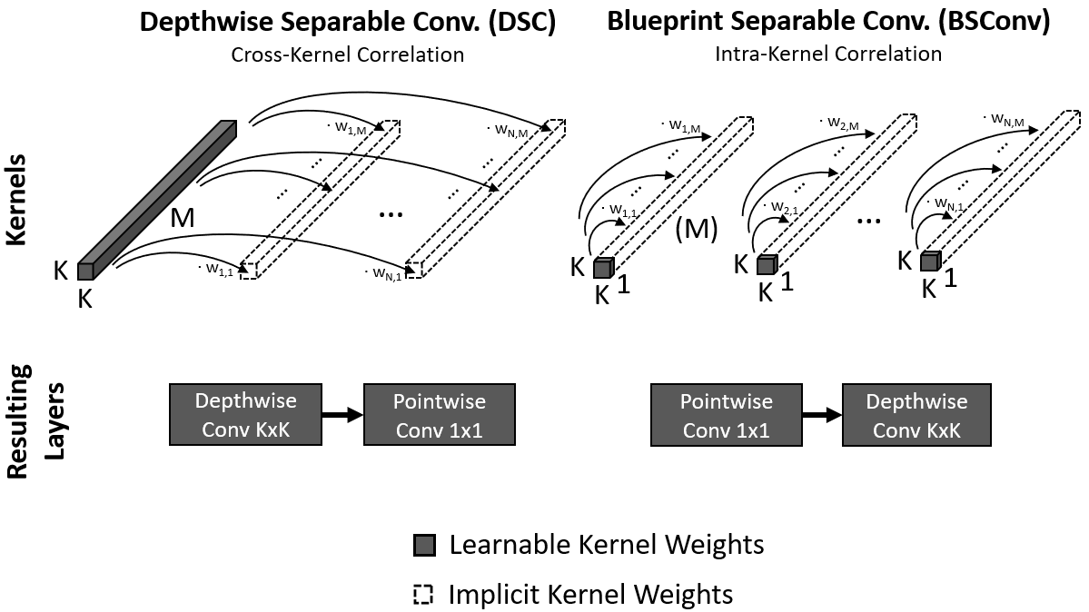
Figure 5: Interpretations for DSC and BSConv. DSCs implicitly assume one 3d blueprint which is used for all kernels, while BSConv relies on individual 2d blueprints for each kernel.

The MobileNetV1 architecture can be translated to a BSConv-U model by simply substituting all DSCs by BSConv-U building blocks, which effectively means switching the order depthwise and pointwise convolutions. However, the inversion of the layer order should have no substantial effect on the middle flow of the network, since we already have alternating point- and depthwise convolutions. The main difference comes from the entry flow: with our approach, feature maps from the first regular convolution can be fully utilized by the depthwise convolution via the preceding pointwise distribution. In contrast, each kernel of the first depthwise convolution of the original MobileNetV1 model can only benefit from a single feature map, leading to limited expressiveness. Following our derivation, for the BSConv-U version of MobileNetV1, no activation nor normalization is applied after the pointwise convolutions, since it is essential to allow the weights $w_{n,m}$ to be negative.

4.2 BSConv-S is a Shifted Linear Bottleneck with Orthonormal Regularization

Linear bottlenecks with inverted residual skips were first introduced in [35] as a highly efficient building block providing impressive expressiveness at a minimum amount of required operations. It follows the idea of regularizing bottlenecks in very large ResNets and became the de facto standard in most of the current state-of-the-art mobile architectures such as MobileNetV2 and MobileNetV3. A single block consists of a cascade of a pointwise, a depthwise, and a pointwise convolution where the bottleneck is placed between blocks. Considering BSConv-S, we can see the close relationship when shifting our cascade of two pointwise and one depthwise convolution within a block to obtain a pointwise, a depthwise, and a pointwise convolution. Thus, MobileNetV2 and V3 can be reinterpreted as a BSConv model with subspace transforms. As found by [35], the shift of residual skips into the bottleneck provides superior model performance and we keep that idea also for our implementation of MobileNets equipped with BSConv-S. Following our derivation in Section 3.3.2, the linear bottleneck, i.e. without the use of an activation function, comes quite natural since negative components are equally essential as positive ones for the subspace transform. Note that this implies that the first bottleneck block does not apply a subspace transform while the last feature map before the final classification layer is in fact compressed. Most importantly, BSConv-S models greatly benefit from our theoretical findings concerning the application of the orthonormal regularization during training. Note that the conversion to a BSConv-S model as described above is also suited for other architectures which use linear bottleneck blocks, such as EfficientNet [41] and MnasNet [40].

5 Experiments

We evaluate our approach of blueprint separable convolutions based on a variety of commonly used benchmark datasets. We provide a comprehensive analysis of the MobileNet family and their modified counterparts according to our findings in Section 4. Furthermore, we demonstrate how our approach can be used as a drop-in substitution for regular convolution layers in standard models like ResNets to drastically reduce the number of model parameters and operations, while keeping or even gaining accuracy.

To allow for a fair comparison, we train all models—including the baseline networks—with exactly the same training procedure.

5.1 CIFAR10 and CIFAR100

The CIFAR10/100 datasets [25] consist of 50k training and 10k test images of size $32\text{\,px}\times 32\text{\,px}$ and comprise 10 and 100 classes, respectively. As suggested in [13, 45], we train for 200 epochs for both datasets. We use SGD with momentum set to $0.9$ and a weight decay of $10^{-4}$. The initial learning rate is set to $0.1$ and decayed by a factor of $0.1$ at epochs $100$, $150$, and $180$. Images are augmented by random horizontal flips and random shifts by up to $4$ px to prevent models from overfitting [13, 45].

MobileNets. As first experiment, we evaluate our improvements of MobileNetV1–V3 [16, 35, 15] as derived in Section 4. To make MobileNets applicable to CIFAR, we removed the first and second pooling operation to obtain a final feature map of size $4\times 4$. With this modification, we achieve state-of-the-art performance for the baseline models (see Table 1).

As described in Section 4, we use BSConv-U for MobileNetV1 and BSConv-S for MobileNetV2/V3. For the BSConv-S models, we use a subspace compression ratio of $p=\frac{1}{6}$ to have exactly the same parameter count as the vanilla model. The weighting coefficient $\alpha$ for the orthonormal regularization loss was set to $0.01$.

Network	CIFAR10		CIFAR100		Stanford Dogs		Stanford Cars		Oxford Flowers
	orig	ours	orig	ours	orig	ours	orig	ours	orig	ours
MobileNetV1 (x0.25)	90.4	91.6	67.5	69.8	42.8	49.1	64.6	74.0	59.2	68.0
MobileNetV1 (x0.5)	91.8	93.3	70.8	73.5	49.3	55.2	70.6	78.8	63.1	71.5
MobileNetV1 (x0.75)	92.7	94.3	72.2	74.5	51.4	57.9	72.9	80.0	63.1	70.8
MobileNetV1 (x1.0)	93.4	94.3	73.4	75.7	51.6	59.1	74.4	79.9	60.2	67.3
MobileNetV2 (x0.25)	89.6	90.1	65.6	68.9	42.0	46.8	65.2	69.9	44.9	51.9
MobileNetV2 (x0.5)	92.0	93.2	72.5	73.2	50.8	54.8	70.4	78.0	57.6	60.6
MobileNetV2 (x0.75)	93.1	93.9	73.2	75.0	53.5	59.0	73.4	82.0	55.7	71.5
MobileNetV2 (x1.0)	93.6	94.2	74.9	75.8	56.0	60.1	76.7	83.8	61.3	67.0
MobileNetV3-small (x0.35)	90.3	90.6	66.5	67.2	42.8	44.2	63.4	70.4	56.9	66.5
MobileNetV3-small (x0.5)	91.5	91.7	69.4	69.6	45.3	47.4	68.1	74.4	64.0	71.7
MobileNetV3-small (x0.75)	92.0	92.5	70.4	72.0	46.7	49.5	72.1	77.2	66.3	74.3
MobileNetV3-small (x1.0)	92.2	92.7	72.2	73.7	49.4	52.1	72.5	77.0	68.4	75.6
MobileNetV3-large (x0.35)	92.8	93.0	71.5	73.7	48.5	56.0	69.5	77.5	55.7	69.4
MobileNetV3-large (x0.5)	93.0	93.9	72.9	75.3	51.2	57.9	73.6	80.4	65.7	66.8
MobileNetV3-large (x0.75)	93.7	94.4	73.9	77.0	51.8	60.0	74.9	80.9	63.1	75.1
MobileNetV3-large (x1.0)	93.7	94.6	75.2	77.7	54.9	60.0	75.7	82.3	64.4	73.8

Table 1: MobileNet results for various datasets. The columns ‘orig’ refer to the baseline MobileNet models. The columns ‘ours’ refer to BSConv-U for MobileNetV1 and BSConv-S for MobileNetV2/V3.

The results are shown in Table 1. We can state that all BSConv variants outperform their corresponding MobileNet baselines. For MobileNetV1, this can be explained by (i) the inversion of point- and depthwise convolutions and (ii) the absence of ReLU activations for the pointwise convolutions (see discussion in Section 4.1). For MobileNetsV2 and V3, the fact that BSConv-S always outperforms the baseline models clearly confirms the advantage of our proposed orthonormal regularization loss.

ResNets and WideResNets. In addition to the improvements with respect to MobileNets, we can use our BSConv approach as drop-in substitution for regular convolution layers in standard networks. In the following, we consider ResNets [13] and WideResNets [45] as two state-of-the-art models for the CIFAR datasets. In both cases, we use the BSConv-U variant. We increase the depth and width factor of each BSConv model such that its parameter count matches the parameter count of the corresponding baseline model. We apply the same training protocol and augmentation techniques as described above.

Network	CIFAR10			CIFAR100
	Parameters	FLOPs	Accuracy	Parameters	FLOPs	Accuracy
ResNet-20 [13]	272.5K	41.3M	92.2	278.3K	41.3M	67.7
ResNet-110 (BSConv-U)	239.0K	41.1M	92.9	244.8K	41.1M	70.8
WideResNet-40-3 [45]	5.0M	735.0M	94.9	5.0M	735.0M	75.5
WideResNet-40-8 (BSConv-U)	4.2M	671.6M	95.2	4.3M	671.6M	77.6

Table 2: ResNets and WideResNets on CIFAR10 and CIFAR100. We increase the depth and width factor of each BSConv model such that its parameter count matches the parameter count of the corresponding baseline model.

In Table 2 we compare the original networks with their modified BSConv versions. For ResNets, we can improve accuracy by up to $3.1$ percentage points for CIFAR100, while having slightly fewer parameters and computational costs. For WideResNets, we can gain accuracy of up to $2.1$ percentage points for CIFAR100, while having fewer parameters and computational costs. This clearly shows the effectiveness of our approach as an drop-in substitution of regular convolution layers.

5.2 ImageNet

To assess the performance of BSConv models in large-scale classification scenarios, we conduct experiments on the ImageNet dataset (ILSVRC2012, [34]). It contains about 1.3M images for training and 50k images for testing which are drawn from 1000 object categories.

We employ a common training protocol and train for 100 epochs with an initial learning rate of $0.1$ which is decayed by a factor of $0.1$ at epochs $30$, $60$, and $90$. We use SGD with momentum $0.9$ and a weight decay of $10^{-4}$. To allow for a fair comparison and to investigate the effect of our approach, we train own baseline models with exactly the same training setup as used for BSConv models. The images are resized such that their short side has a length of $256$ px. We use the well-established Inception-like scale augmentation [39], horizontal flips, and color jitter [26].

MobileNets. As for the CIFAR experiments, we compare MobileNets to their corresponding BSConv variants. Again, BSConv-U is used for MobileNetV1, and BSConv-S is used for MobileNetV2/V3. The subspace compression ratio for BSConv-S is $p=\frac{1}{6}$ just like for the CIFAR experiments. The weighting coefficient $\alpha$ for the orthonormal regularization loss was set to $0.1$.

Network	Original	BSConv (ours)
MobileNetV1 (x0.25)	51.8	53.2
MobileNetV1 (x0.5)	63.5	64.6
MobileNetV1 (x0.75)	68.2	69.2
MobileNetV1 (x1.0)	70.8	71.5
MobileNetV2 (x1.0)	69.7	69.8
MobileNetV3-small (x1.0)	64.4	64.8
MobileNetV3-large (x1.0)	71.5	71.5

Table 3: MobileNets on ImageNet. BSConv-U is used for MobileNetV1, and BSConv-S is used for MobileNetV2/V3. Note that BSConv does not introduce additional parameters.

The results are presented in Table 3. Again, it can be seen that the BSConv variants of MobileNets outperform their corresponding baseline models. However, the relative improvements are no longer as large as for the CIFAR experiments. This effect can be explained by the regularization impact of the dataset itself. Considering the MobileNetV3-large results, we note that even if the orthonormal regularization loss seems to be no longer effective, it has no negative influence on the training.

ResNets. As noted before, it is possible to directly substitute regular convolution layers in standard networks by BSConv variants. To this end, we analyze the effectiveness of our approach when applied to ResNets on large-scale image databases. For the baseline models, we use ResNet-10, ResNet-18, and ResNet-26. The BSConv variants are ResNet-10, ResNet-18, ResNet-34, ResNet-68, and ResNet-102. Again, we use the same training protocol and augmentation techniques as described above.

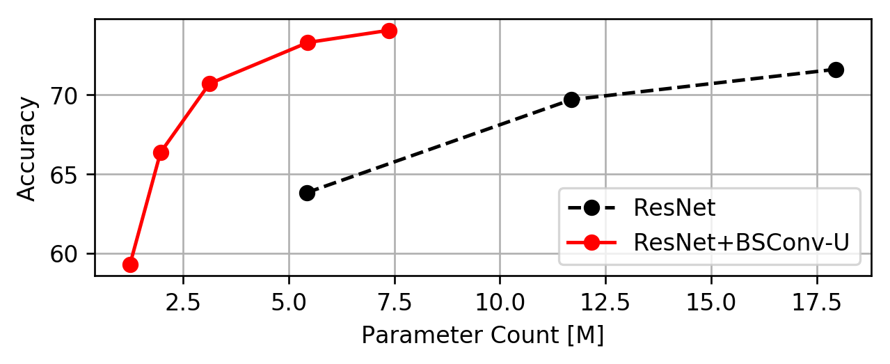
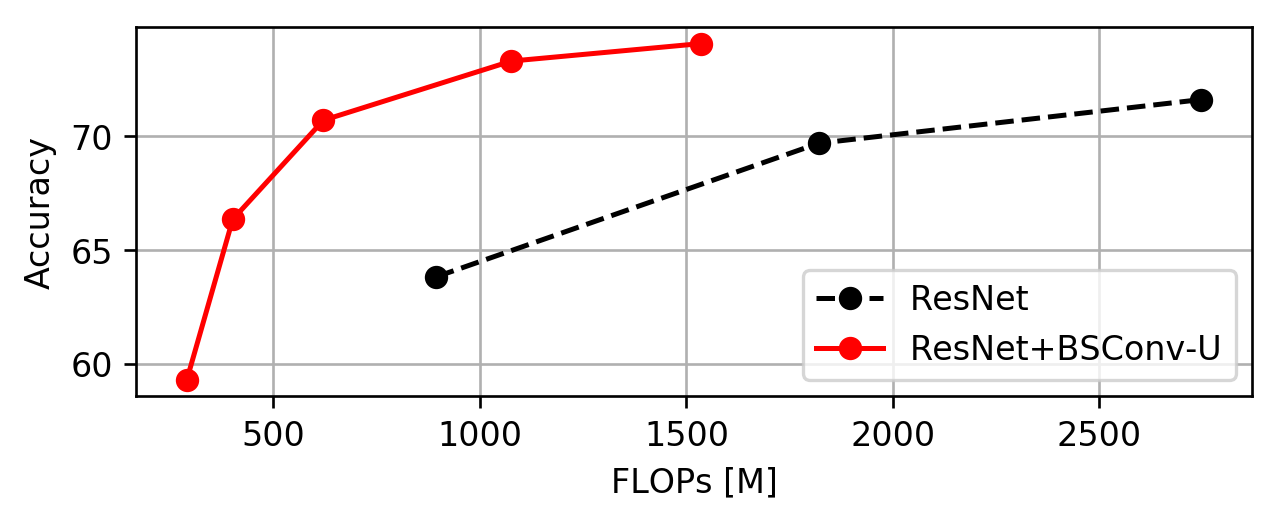
Figure 6: ResNets on ImageNet. For the baseline models, we use ResNet-10/18/26. The BSConv variants are ResNet-10/18/34/68/102.

The results are shown in Figure 6, split by parameter count and computational complexity. It can be seen that the BSConv-U variants of ResNets significantly outperform the baseline models. ResNet-10 and ResNet-68+BSConv-U, for instance, have similar parameter counts, while using BSConv leads to an accuracy gain of $9.5$ percentage points. Another interesting example is ResNet-18 vs. ResNet-34+BSConv-U: both have a comparable accuracy, while the BSConv model has only about one fifth of the baseline model parameter count.

5.3 Fine-grained Recognition

Apart from large-scale object recognition, we are interested in the task of fine-grained classification, as those datasets usually have no inherent regularization. The following experiments are conducted on three well-established benchmark datasets for fine-grained recognition, namely Stanford Dogs [23], Stanford Cars [24], and Oxford 102 Flowers [32]. We train all models from scratch, since parts of these datasets are a subset of ImageNet. In contrast to the ImageNet training protocol, we do not use aggressive data augmentation, since we observed that it severely affects model performance. We only augment data via random crops, horizontal flips, and random gamma transform.

We use the same training protocol for all three datasets. In particular, we use SGD with momentum set to $0.9$ and a weight decay of $10^{-4}$. The initial learning rate is set to $0.1$ and linearly decayed at every epoch such that it approaches zero after a total of $100$ epochs.

MobileNets. We use the same model setup as for the CIFAR and ImageNet experiments discussed above. The results are shown in Table 1. Again, all BSConv models substantially outperform their baseline counterparts. In contrast to the CIFAR results, the margin is even larger. Therefore, the interpretation of the CIFAR results applies here as well.

Other Architectures. We further evaluate the effect of our approach for a variety of state-of-the-art models. We replace regular convolution layers in standard networks such as VGG [38] and DenseNet [17].

In Table 4 we can see that all models greatly benefit from the application of BSConv. Accuracy for BSConv-U can be improved by at least 2 percentage points, while having up to $8.5\times$ less parameters and a substantial reduction of computational complexity. Most of the recently proposed model architectures utilize residual linear bottlenecks [35], which can also be easily equipped with our BSConv-S approach in the same way as for MobileNetV2/V3 (see Section 4.2). As can be seen in Table 4, our subspace model clearly outperforms the original EfficientNet-B0 [41] by $6.5$ percentage points and MnasNet [40] by $5$ percentage points with the same number of parameters and computational complexity. This shows the effectiveness of our proposed orthonormal regularization of the BSConv-S subspace transform.

Network	Accuracy
VGG-16 (BN) [38]	60.5
VGG-16 (BN) (BSConv-U)	62.4
DenseNet-121 [17]	56.9
DenseNet-121 (BSConv-U)	59.4
Xception* [2]	59.6
Xception (BSConv-U)	64.3
EfficientNet-B0 [41]	54.7
EfficientNet-B0 (BSConv-S)	61.2
MnasNet [40]	54.8
MnasNet (BSConv-S)	59.8

Table 4: Results of various architectures and their BSConv counterparts for the Stanford Dogs dataset. BSConv-U CNNs have fewer parameters and a smaller computational complexity compared to their baseline models. BSConv-S CNNs have the same parameter count and computational complexity as their counterparts. * Commonly used implementation based on DSCs.

Influence of the Orthonormal Regularization. To evaluate the influence of the proposed orthonormal regularization loss for BSConv-S models, we conduct an ablation study using MobileNetV3-large. In particular, several identical models are trained on the Stanford Dogs dataset using weighting coefficients $\alpha$ in the range of $10^{-5},\ldots,10^{0}$.

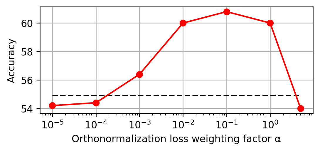
Figure 7: Influence of the orthonormal regularization loss on the accuracy for the BSConv-S variant of MobileNetV3-large (red solid line) on Stanford Dogs. The baseline MobileNetV3-large model without BSConv-S is indicated by the black dashed line.

As can be seen in Figure 7, by regularizing the subspace components to be orthonormal, model performance can be substantially improved by over $5$ percentage points. An optimum is reached for a weighting coefficient of $\alpha=0.1$. For smaller values, the influence of the regularization decreases, until it is no longer effective and converges towards the baseline performance. Larger values, however, decrease model performance since the optimization is mainly driven by rapidly reaching a solution with an orthonormal basis independently of creating a beneficial joint representation.

6 Conclusions

We introduced blueprint separable convolutions (BSConv) as highly efficient building blocks for CNNs. Our formulation provided an interpretation and justification for depthwise separable convolutions. By using BSConv, we clearly and consistently improved established models such as MobileNets, MnasNets, EfficientNets, and ResNets. Code and trained models are available under https://github.com/zeiss-microscopy/BSConv.

References

- [1] Han Cai, Ligeng Zhu, and Song Han. Proxylessnas: Direct neural architecture search on target task and hardware. arXiv preprint arXiv:1812.00332, 2018.
- [2] François Chollet. Xception: Deep learning with depthwise separable convolutions. In Proceedings of the IEEE conference on computer vision and pattern recognition, pages 1251–1258, 2017.
- [3] Misha Denil, Babak Shakibi, Laurent Dinh, Marc’Aurelio Ranzato, and Nando De Freitas. Predicting parameters in deep learning. In Advances in neural information processing systems, pages 2148–2156, 2013.
- [4] Emily L Denton, Wojciech Zaremba, Joan Bruna, Yann LeCun, and Rob Fergus. Exploiting linear structure within convolutional networks for efficient evaluation. In Advances in neural information processing systems, pages 1269–1277, 2014.
- [5] Ross Girshick, Jeff Donahue, Trevor Darrell, and Jitendra Malik. Rich feature hierarchies for accurate object detection and semantic segmentation. In Proceedings of the IEEE conference on computer vision and pattern recognition, pages 580–587, 2014.
- [6] Yunchao Gong, Liu Liu, Ming Yang, and Lubomir Bourdev. Compressing deep convolutional networks using vector quantization. arXiv preprint arXiv:1412.6115, 2014.
- [7] Jianbo Guo, Yuxi Li, Weiyao Lin, Yurong Chen, and Jianguo Li. Network decoupling: From regular to depthwise separable convolutions. arXiv preprint arXiv:1808.05517, 2018.
- [8] Song Han, Xingyu Liu, Huizi Mao, Jing Pu, Ardavan Pedram, Mark A Horowitz, and William J Dally. Eie: efficient inference engine on compressed deep neural network. In 2016 ACM/IEEE 43rd Annual International Symposium on Computer Architecture (ISCA), pages 243–254. IEEE, 2016.
- [9] Song Han, Huizi Mao, and William J Dally. Deep compression: Compressing deep neural networks with pruning, trained quantization and huffman coding. arXiv preprint arXiv:1510.00149, 2015.
- [10] Song Han, Jeff Pool, John Tran, and William Dally. Learning both weights and connections for efficient neural network. In Advances in neural information processing systems, pages 1135–1143, 2015.
- [11] Babak Hassibi and David G Stork. Second order derivatives for network pruning: Optimal brain surgeon. In Advances in neural information processing systems, pages 164–171, 1993.
- [12] Kaiming He and Jian Sun. Convolutional neural networks at constrained time cost. In Proceedings of the IEEE conference on computer vision and pattern recognition, pages 5353–5360, 2015.
- [13] Kaiming He, Xiangyu Zhang, Shaoqing Ren, and Jian Sun. Deep residual learning for image recognition. In Proceedings of the IEEE conference on computer vision and pattern recognition, pages 770–778, 2016.
- [14] Kaiming He, Xiangyu Zhang, Shaoqing Ren, and Jian Sun. Identity mappings in deep residual networks. In European conference on computer vision, pages 630–645. Springer, 2016.
- [15] Andrew Howard, Mark Sandler, Grace Chu, Liang-Chieh Chen, Bo Chen, Mingxing Tan, Weijun Wang, Yukun Zhu, Ruoming Pang, Vijay Vasudevan, et al. Searching for mobilenetv3. arXiv preprint arXiv:1905.02244, 2019.
- [16] Andrew G Howard, Menglong Zhu, Bo Chen, Dmitry Kalenichenko, Weijun Wang, Tobias Weyand, Marco Andreetto, and Hartwig Adam. Mobilenets: Efficient convolutional neural networks for mobile vision applications. arXiv preprint arXiv:1704.04861, 2017.
- [17] Gao Huang, Zhuang Liu, Laurens Van Der Maaten, and Kilian Q Weinberger. Densely connected convolutional networks. In Proceedings of the IEEE conference on computer vision and pattern recognition, pages 4700–4708, 2017.
- [18] Yanping Huang, Yonglong Cheng, Dehao Chen, HyoukJoong Lee, Jiquan Ngiam, Quoc V Le, and Zhifeng Chen. Gpipe: Efficient training of giant neural networks using pipeline parallelism. arXiv preprint arXiv:1811.06965, 2018.
- [19] Itay Hubara, Matthieu Courbariaux, Daniel Soudry, Ran El-Yaniv, and Yoshua Bengio. Quantized neural networks: Training neural networks with low precision weights and activations. The Journal of Machine Learning Research, 18(1):6869–6898, 2017.
- [20] Sergey Ioffe and Christian Szegedy. Batch normalization: Accelerating deep network training by reducing internal covariate shift. arXiv preprint arXiv:1502.03167, 2015.
- [21] Max Jaderberg, Andrea Vedaldi, and Andrew Zisserman. Speeding up convolutional neural networks with low rank expansions. arXiv preprint arXiv:1405.3866, 2014.
- [22] Jonghoon Jin, Aysegul Dundar, and Eugenio Culurciello. Flattened convolutional neural networks for feedforward acceleration. arXiv preprint arXiv:1412.5474, 2014.
- [23] Aditya Khosla, Nityananda Jayadevaprakash, Bangpeng Yao, and Li Fei-Fei. Novel dataset for fine-grained image categorization. In First Workshop on Fine-Grained Visual Categorization, IEEE Conference on Computer Vision and Pattern Recognition, Colorado Springs, CO, June 2011.
- [24] Jonathan Krause, Michael Stark, Jia Deng, and Li Fei-Fei. 3d object representations for fine-grained categorization. In 4th International IEEE Workshop on 3D Representation and Recognition (3dRR-13), Sydney, Australia, 2013.
- [25] Alex Krizhevsky, Geoffrey Hinton, et al. Learning multiple layers of features from tiny images. Technical report, Citeseer, 2009.
- [26] Alex Krizhevsky, Ilya Sutskever, and Geoffrey E Hinton. Imagenet classification with deep convolutional neural networks. In Advances in neural information processing systems, pages 1097–1105, 2012.
- [27] Yann LeCun, Bernhard Boser, John S Denker, Donnie Henderson, Richard E Howard, Wayne Hubbard, and Lawrence D Jackel. Backpropagation applied to handwritten zip code recognition. Neural computation, 1(4):541–551, 1989.
- [28] Hao Li, Asim Kadav, Igor Durdanovic, Hanan Samet, and Hans Peter Graf. Pruning filters for efficient convnets. arXiv preprint arXiv:1608.08710, 2016.
- [29] Zhuang Liu, Mingjie Sun, Tinghui Zhou, Gao Huang, and Trevor Darrell. Rethinking the value of network pruning. arXiv preprint arXiv:1810.05270, 2018.
- [30] Jonathan Long, Evan Shelhamer, and Trevor Darrell. Fully convolutional networks for semantic segmentation. In Proceedings of the IEEE conference on computer vision and pattern recognition, pages 3431–3440, 2015.
- [31] Ningning Ma, Xiangyu Zhang, Hai-Tao Zheng, and Jian Sun. Shufflenet v2: Practical guidelines for efficient cnn architecture design. In Proceedings of the European Conference on Computer Vision (ECCV), pages 116–131, 2018.
- [32] Maria-Elena Nilsback and Andrew Zisserman. Automated flower classification over a large number of classes. In 2008 Sixth Indian Conference on Computer Vision, Graphics & Image Processing, pages 722–729. IEEE, 2008.
- [33] Mohammad Rastegari, Vicente Ordonez, Joseph Redmon, and Ali Farhadi. Xnor-net: Imagenet classification using binary convolutional neural networks. In European Conference on Computer Vision, pages 525–542. Springer, 2016.
- [34] Olga Russakovsky, Jia Deng, Hao Su, Jonathan Krause, Sanjeev Satheesh, Sean Ma, Zhiheng Huang, Andrej Karpathy, Aditya Khosla, Michael Bernstein, et al. Imagenet large scale visual recognition challenge. International journal of computer vision, 115(3):211–252, 2015.
- [35] Mark Sandler, Andrew Howard, Menglong Zhu, Andrey Zhmoginov, and Liang-Chieh Chen. Mobilenetv2: Inverted residuals and linear bottlenecks. In Proceedings of the IEEE Conference on Computer Vision and Pattern Recognition, pages 4510–4520, 2018.
- [36] Wenling Shang, Kihyuk Sohn, Diogo Almeida, and Honglak Lee. Understanding and improving convolutional neural networks via concatenated rectified linear units. In international conference on machine learning, pages 2217–2225, 2016.
- [37] L Sifre and S Mallat. Rigid-motion scattering for image classification, 2014. PhD thesis, Ph. D. thesis, 2014.
- [38] Karen Simonyan and Andrew Zisserman. Very deep convolutional networks for large-scale image recognition. arXiv preprint arXiv:1409.1556, 2014.
- [39] Christian Szegedy, Wei Liu, Yangqing Jia, Pierre Sermanet, Scott Reed, Dragomir Anguelov, Dumitru Erhan, Vincent Vanhoucke, and Andrew Rabinovich. Going deeper with convolutions. In Proceedings of the IEEE conference on computer vision and pattern recognition, pages 1–9, 2015.
- [40] Mingxing Tan, Bo Chen, Ruoming Pang, Vijay Vasudevan, Mark Sandler, Andrew Howard, and Quoc V Le. Mnasnet: Platform-aware neural architecture search for mobile. In Proceedings of the IEEE Conference on Computer Vision and Pattern Recognition, pages 2820–2828, 2019.
- [41] Mingxing Tan and Quoc V Le. Efficientnet: Rethinking model scaling for convolutional neural networks. arXiv preprint arXiv:1905.11946, 2019.
- [42] Min Wang, Baoyuan Liu, and Hassan Foroosh. Factorized convolutional neural networks. In Proceedings of the IEEE International Conference on Computer Vision, pages 545–553, 2017.
- [43] Lingxi Xie and Alan Yuille. Genetic cnn. In Proceedings of the IEEE International Conference on Computer Vision, pages 1379–1388, 2017.
- [44] Saining Xie, Ross Girshick, Piotr Dollár, Zhuowen Tu, and Kaiming He. Aggregated residual transformations for deep neural networks. In Proceedings of the IEEE conference on computer vision and pattern recognition, pages 1492–1500, 2017.
- [45] Sergey Zagoruyko and Nikos Komodakis. Wide residual networks. arXiv preprint arXiv:1605.07146, 2016.
- [46] Xiangyu Zhang, Xinyu Zhou, Mengxiao Lin, and Jian Sun. Shufflenet: An extremely efficient convolutional neural network for mobile devices. In Proceedings of the IEEE Conference on Computer Vision and Pattern Recognition, pages 6848–6856, 2018.
- [47] Aojun Zhou, Anbang Yao, Yiwen Guo, Lin Xu, and Yurong Chen. Incremental network quantization: Towards lossless cnns with low-precision weights. arXiv preprint arXiv:1702.03044, 2017.
- [48] Barret Zoph and Quoc V Le. Neural architecture search with reinforcement learning. arXiv preprint arXiv:1611.01578, 2016.