A piecewise linear model of self-organized hierarchy formation

Abstract

The Bonabeau model of self-organized hierarchy formation is studied by using a piecewise linear approximation to the sigmoid function. Simulations of the piecewise-linear agent model show that there exist two-level and three-level hierarchical solutions, and that each agent exhibits a transition from non-ergodic to ergodic behaviors. Furthermore, by using a mean-field approximation to the agent model, it is analytically shown that there are asymmetric two-level solutions, even though the model equation is symmetric (asymmetry is introduced only through the initial conditions), and that linearly stable and unstable three-level solutions coexist. It is also shown that some of these solutions emerge through supercritical-pitchfork-like bifurcations in invariant subspaces. Existence and stability of the linear hierarchy solution in the mean-field model are also elucidated.

I Introduction

Hierarchy formation has been intensively studied in a wide range of animal species: insects Oliveira and Holldobler (1990), fish Goessmann et al. (2000); Chase et al. (2002); Grosenick et al. (2007), birds Lindquist and Chase (2009), and mammals Wittig and Boesch (2003) including even humans Savin-Williams (1980); Garandeau et al. (2014). It has been considered that not only differences in the prior attributes of individuals such as weight and aggressiveness but also social interactions between individuals are important in the hierarchy formation Chase et al. (2002); Castellano et al. (2009). In fact, it is known that an individual who won an earlier contest has a higher probability of winning later contests than an individual who lost the earlier contest (winner-loser effects) Hsu et al. (2006). Positive feedback generated through such effects might enhance the formation of hierarchies in animal groups.

To elucidate such a feedback mechanism in hierarchy formations, a mathematical model is proposed by Bonabeau et al Bonabeau et al. (1995). The Bonabeau model consists of $N$ agents, and each agent $i\,(i=1,\dots,N)$ is characterized by a variable $F_{i}(t)$, where $t$ is time. $F_{i}(t)$, which is called strength or fitness in the literature, is referred to as a dominance score (DS) in this paper Lindquist and Chase (2009). After a contest between two agents $i$ and $j$, $F_{i}(t)$ increases if the agent $i$ wins and decreases if $i$ loses [the same rule is applied to $F_{j}(t)$]. A greater value of $F_{i}(t)$ means a higher probability to win a contest. In addition, the agents are assumed to perform random walks on a two-dimensional square lattice $L\times L$, and a contest occurs when two agents meet; thus, the density of the agents $\rho=N/L^{2}$ is a parameter, which controls the frequency of contests. In addition to these pairwise interactions, $F_{i}(t)$ is assumed to show a relaxation according to a differential equation $dF_{i}(t)/dt=-\mu\tanh\bigl{(}F_{i}(t)\bigr{)}$.

It is found that, as the density $\rho$ increases, the Bonabeau model shows a transition from an egalitarian state in which all $F_{i}(t)$ are equal to a hierarchical state in which $F_{i}(t)\neq F_{j}(t)$ for some $i\neq j$. The Bonabeau model is one of the basic models of the hierarchy formation, and it is compared with experimental observations of hierarchies in animal groups Bonabeau et al. (1999); Lindquist and Chase (2009). Hierarchical structures can be well described by the Bonabeau model Bonabeau et al. (1999), but some discrepancies are also reported Lindquist and Chase (2009).

Since the Bonabeau model is a simple model, many modified versions have been proposed to make it more realistic. In Refs. Stauffer (2003); Stauffer and Sa Martins (2003), another feedback mechanism and an asymmetric rule are incorporated into the dynamics of $F_{i}(t)$. This generalized model (a Stauffer version) is analyzed in Ref. Lacasa and Luque (2006), and it was found that the egalitarian solution is always stable, while a two-level stable solution (a hierarchical solution) appears at a critical parameter value through a saddle-node bifurcation. In addition, a model with a simpler relaxation dynamics $dF_{i}(t)/dt=-\mu F_{i}(t)$ is also analyzed in Ref. Lacasa and Luque (2006), and it was found that a similar transition occurs but in this case the bifurcation is supercritical-pitchfork type. Recently, an asymmetric model is intensively studied in Ref. Pósfai and D’Souza ; In this asymmetric model, each agent has an intrinsic parameter called a talent, which can be considered as a prior attribute of that agent. Moreover, two modified models are proposed in Refs.Odagaki and Tsujiguchi (2006); Tsujiguchi and Odagaki (2007); Okubo and Odagaki (2007): a timid-society model and a challenging-society model. In the timid-society model, an agent can choose a vacant site when it moves and thereby it can avoid a contest; in the challenging-society model, the agent chooses the strongest neighbor as an opponent.

In contrast to these modifications trying to incorporate realistic features, there are also works intending to simplify the Bonabeau model Ben-Naim and Redner (2005); Ben-Naim et al. (2006, 2007). In these studies, the DSs of agents are assumed to attain only integer values, and the DS of the winner increases by one and that of the loser does not change. The dynamics can be described by a partial differential equation in a continuum limit. This model also shows a transition from the egalitarian solution to a hierarchical solution.

In spite of this diversity of models of the hierarchy formation, understanding of the original Bonabeau model is still limited. For example, in the Bonabeau model with relaxation dynamics $dF_{i}(t)/dt=-\mu F_{i}(t)$, it is found that the egalitarian solution is stable at low densities (at small values of $\rho$). This egalitarian solution becomes unstable at $\rho=\rho_{c}$, and two-level stable solutions appear through a supercritical-pitchfork bifurcation Lacasa and Luque (2006). But, it seems impossible to rigorously derive the stable range of this two-level solution (some approximation is necessary). This difficulty stems mainly from nonlinearity of the sigmoid function employed in the Bonabeau model (See Sec. II).

In this paper, we propose another simplified version of the Bonabeau model by introducing a piecewise linear function in place of the sigmoid function. Piecewise linear approximations are often used in the studies of nonlinear dynamical systems. In fact, even for systems in which rigorous approaches are difficult, more detailed analysis is possible for piecewise linear versions Devaney (1984); Tasaki and Gaspard (2002); Miyaguchi (2006); Miyaguchi and Aizawa (2007). Here, we derive the stable ranges of two-level and three-level solutions for the piecewise-linear model. Moreover, we found that asymmetric two-level solutions exist even though the system is symmetric (asymmetry is introduced only through the initial conditions). It is also shown that various stable and unstable solutions coexist.

This paper is organized as follows. In Sec. II, we define two piecewise-linear models of the hierarchy formation: an agent model and a mean-field model. In Sec. III, linear stability analysis for steady solutions (i.e., fixed points Strogatz (1994)) of the mean-field model is presented. In Sec. IV, a transition from ergodic to non-ergodic behaviors in the agent model is numerically studied. Finally, Sec. V is devoted to a discussion, in which we suggest possible generalizations of the agent model.

II Models

In this section, we introduce two models of the self-organized hierarchy formation. The first model is referred to as an agent model, and the second as a mean-field model. It is shown that the mean-field model is a good approximation of the agent model in a weak interaction limit.

II.1 Agent model

Let us suppose that there are $N$ agents, and each agent $i\,\,(i=1,\dots,N)$ is characterized by a real number $F_{i}(t)$, which is referred to as the DS at time $t$ Bonabeau et al. (1995). $F_{i}(t)$ is a measure of strength or fitness of the agent $i$ Castellano et al. (2009); Lacasa and Luque (2006), and changes through interactions with other agents; Hereafter, the interaction between two agents is referred to as a contest. Firstly, we define the dynamics just at the contest; Secondly, we define inter-contest dynamics by using a Poisson process.

Figure 1: Probabilities of the gain $F_{i}(t_{n}^{+})-F_{i}(t_{n}^{-})$ (a) for the model defined in Eq. (1), and (b) for the Bonabeau model. Here, $x$ stands for the difference of the DSs of two contestants, e.g., $x=F_{i}(t^{-}_{n})-F_{j}(t^{-}_{n})$. Then, $q(x)\,[q(-x)]$ is the probability that the agent $i$ wins (loses) the contest with $j$. The mean gain $\mu$ is expressed as $\mu=\eta[q(x)-q(-x)]=\eta f(x)$ [Eq. (8)].

II.1.1 Contest dynamics

Let us define the dynamics of $F_{i}(t)$ at the contests. At random time $t=t_{n}$, two agents $i$ and $j$ contest with each other, where $i$ and $j$ are randomly chosen from the $N$ agents. In this contest, the values of $F_{i}(t)$ and $F_{j}(t)$ change as

$$F_{i}(t_{n}^{+}) =F_{i}(t_{n}^{-})+\eta f\bigl{(}F_{i}(t^{-}_{n})-F_{j}(t^{-}_{n})\bigr{)}+\xi_{i}(t_{n}),$$ (1)

$$F_{j}(t_{n}^{+}) =F_{j}(t_{n}^{-})+\eta f\bigl{(}F_{j}(t^{-}_{n})-F_{i}(t^{-}_{n})\bigr{)}+\xi_{j}(t_{n}),$$ (2)

where $t_{n}^{-}$ and $t_{n}^{+}$ are the times just before and after the contest, respectively. A gain from winning or losing the contest is defined by the difference of the DSs before and after the contest, $F_{i}(t_{n}^{+})-F_{i}(t_{n}^{-})$, which is equivalent to the sum of the second and the third terms in the right side of Eq. (1). Therefore, the parameter $\eta$ controls the amount of the gain, thereby characterizing the impact of the contest result. Moreover, $\xi_{i}(t)$ is a random variable following the normal distribution with mean $0$ and variance $\sigma^{2}$, and satisfies an independence property $\left\langle\xi_{i}(t_{n})\xi_{j}(t_{m})\right\rangle=\delta_{ij}\delta_{nm}\sigma^{2}$. The gain is thus a random variable, and its probability density is illustrated in Fig. 1(a).

In Eqs. (1) and (2), $f(x)$ is a non-linear function similar to the sigmoid function. In this paper, we assume it has the following piecewise linear form:

$$f(x)=\begin{cases}-1&(x\leq-2F_{0}),\\[2.84544pt] \frac{x}{2F_{0}}&(-2F_{0}\leq x\leq 2F_{0}),\\[2.84544pt] 1&(x\geq 2F_{0}),\end{cases}$$ (3)

where $F_{0}$ characterizes the scale of $F_{i}(t)$, and it can be removed by rescaling [See Appendix A]. Note also that $x$ stands for the DS difference of two contestants, e.g., $x=F_{i}(t^{-}_{n})-F_{j}(t^{-}_{n})$ [See Eq. (1)]. This function $f(x)$ is a piecewise-linear approximation to the function

$$f_{\mathrm{b}}(x)=\frac{1}{1+e^{-x/F_{0}}}-\frac{1}{1+e^{x/F_{0}}}.$$ (4)

This function $f_{\mathrm{b}}(x)$ is employed in the original Bonabeau model Bonabeau et al. (1995). Due to the nonlinearity in $f_{\mathrm{b}}(x)$, theoretical analysis of the Bonabeau model is difficult except for a few simple steady solutions. For the piecewise linear approximation given by Eq. (3), however, more detailed analysis of hierarchical solutions is possible due to its simplicity.

The first and the second terms on the right side of Eq. (4) have a simple probabilistic interpretation. Let us define a function $q(x)$ as $q(x):=[f_{b}(x)+1]/2$, then Eq. (4) can be expressed as $f_{b}(x)=q(x)-q(-x)$. If $x$ is given by $x=F_{i}(t^{-}_{n})-F_{j}(t^{-}_{n})$, the first term $q(x)$ is the winning probability of $i$ against $j$, and the second term $q(-x)$ is the losing probability of $i$ against $j$. A similar interpretation is possible also for our model [Eq. (3)]; If we rewrite $f(x)$ as $f(x)=q(x)-q(-x)$ with $q(x)=[f(x)+1]/2$, then $q(x)$ [$q(-x)$] is the probability of winning (losing). Thus, $\eta f(x)$ in the right side of Eq. (1) is the mean gain of the agent $i$ through the contest with $j$.

Apart from this difference in $f(x)$ and $f_{b}(x)$, Eqs. (1) and (2) are still slightly different from the Bonabeau model, for which the dynamics is given by

$$F_{i}(t_{n}^{+})=F_{i}(t_{n}^{-})\pm\eta$$ (5)

with the plus sign if the agent $i$ wins and the minus sign if it loses (a similar equation holds for the opponent). The probabilities of winning and losing are given by $q(x)$ and $q(-x)$ defined above. Thus, the gain of the contest is a random variable following a dichotomous distribution as shown in Fig. 1(b).

The present model shown in Fig. 1(a) can be considered as a coarse-grained version of the Bonabeau model. This is because a sum of several gains, each following the dichotomous distribution in Fig. 1(b), should follow a continuous distribution similar to the one in Fig. 1(a) by virtue of the central limit theorem Feller (1971). Therefore, our model might well be plausible for some species for which the same pair of individuals contest in succession Lindquist and Chase (2009).

More precisely, if we assume that the same pair contests $T$ times in succession in the Bonabeau model, the noise terms in Eqs. (1) and (2) can be considered as small. In fact, the mean and the variance of the sum of the dichotomous gains approximately become

$$\mu \approx T\eta\left[q(x)-q(-x)\right],$$ (6)

$$\sigma^{2} \approx 4T\eta^{2}q(x)q(-x).$$ (7)

Let us rescale $\eta$ by replacing it with $\eta/T$, we obtain

$$\mu \approx\eta\left[q(x)-q(-x)\right],$$ (8)

$$\sigma^{2} \approx\frac{4\eta^{2}}{T}q(x)q(-x).$$ (9)

This is the situation shown in Fig. 1(a). From Eqs. (8) and (9), it is found that, if the timescale $T$ is large, the standard deviation $\sigma$ can be considered as small compared with the mean value $\mu$. Therefore, in the following, we study the simplest case $\sigma^{2}=0$ and neglect the noise terms $\xi_{i}(t)$ and $\xi_{j}(t)$ in Eqs. (1) and (2). Note also that this noiseless model can be considered as a simplification of the Bonabeau model in that the random dichotomous gains $\pm\eta$ in the Bonabeau model are replaced by its mean value $\mu$ given in Eq. (8) [See Fig. 1(b)].

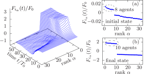
Figure 2: (Left) Two-level hierarchy formation in the agent model with $N=32$. Time evolution of the DS profile $F_{i_{\alpha}}(t)$ is displayed as a function of the rank $\alpha$ and time $t$. Here, $i_{\alpha}(t)$ is the agent index of which rank is $\alpha$ at time $t$. The parameters $\eta$ and $\gamma$ are set as $\eta=10^{-3}F_{0}$ and $\gamma\eta=1.3\rho_{c}$ with $\rho_{c}$ given by Eq. (19). (Right) The initial and final DS profiles are shown in (a) and (b), respectively.

II.1.2 Inter-contest dynamics

In addition to the dynamics just at the contests, we should define the inter-contest dynamics. We assume that the contests occur at random times $t=t_{1},\cdots,t_{n},\cdots$ (we set $t_{0}=0$ for convenience). In the Bonabeau model, the agents are assumed to perform random walks, and the times $t_{n}$ are determined by random encounters of the agents Bonabeau et al. (1995). However, the random walk model introduces non-trivial correlations in the sequence of the intervals $\tau_{n}:=t_{n}-t_{n-1}\,(n=1,2,\dots)$.

Here, however, we assume that these intervals $\tau_{n}$ are mutually independent random variables, and follow the exponential distribution:

$$w(\tau)=\gamma_{a}e^{-\gamma_{a}\tau},$$ (10)

where $\gamma_{a}$ is the interaction rate and its inverse $1/\gamma_{a}$ is the mean of $\tau$. Thus, the inter-contest dynamics is the Poisson process Feller (1971), and simplifies the model dynamics thanks to the independence of the intervals $\tau_{n}$. In the original Bonabeau model, the contest is considered as a diffusion-limited reaction, while the Poisson process might arise from a reaction-limited random walk.

Note that $\gamma_{a}dt$ is the mean number of contests in the time interval $dt$. Then, the mean number of contests in which the agent $i$ involves is $\gamma_{a}dt\times 2/N$. Therefore, let us define $\gamma:=2\gamma_{a}/N$, which is an interaction rate for a single agent. In Appendix A, we show that $\eta$ and $\gamma_{a}$ (or $\gamma$) completely characterize the agent model.

Relaxation of the dominance relationship is observed in experiments of animal groups. For example, in Ref. Chase et al. (2002), a group of fish is assembled to form a hierarchy, then each individual in the group is separated for long time, and finally they are assembled to form a hierarchy again. This second hierarchy is often different from the first, and thus it is considered that individual fish forgets the earlier dominance relationship.

Therefore, in the meantime of the contests in our model, $F_{i}(t)$ is assumed to decay. As a relaxation dynamics, we employ the following differential equation:

$$\frac{dF_{i}(t)}{dt}=-\frac{F_{i}(t)}{T_{0}}.$$ (11)

Here, $T_{0}>0$ is a characteristic time scale of the relaxation, and it can be removed by rescaling (See Appendix A).

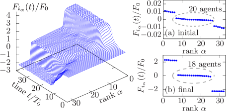
Figure 3: (Left) Three-level hierarchy formation in the agent model with $N=32$. Time evolution of the DS profile $F_{i_{\alpha}}(t)$ is displayed as a function of the rank $\alpha$ and time $t$. The parameters $\eta$ and $\gamma$ are set as $\eta=10^{-3}F_{0}$ and $\gamma\eta=1.5\rho_{c}$ with $\rho_{c}$ given by Eq. (19). (Right) The initial and final DS profiles are shown in (a) and (b), respectively.

In Figs. 2 and 3, results of numerical simulations for the agent model are presented. In these simulations, we neglect the noise terms $\xi_{i}(t)$ (i.e., we set $\sigma^{2}=0$). The initial condition $F_{i}(0)$ is weakly stratified into two and three groups as shown in Figs. 2(a) and 3(a), respectively. At long times, the DS profile $F_{i}(t)$ converges to stratified profiles slightly different from the initial profiles (but there are some fluctuations at the final states due to stochastic dynamics, i.e., the random sampling of the contestants, and the random intervals $\tau_{n}$). As shown in Fig. 2(b), the final state is an asymmetric two-level profile, whereas in Fig. 3(b), the final state is a symmetric three-level profile. In addition, even if the parameters are the same, there are several final profiles depending only on the initial conditions and realizations of the stochastic dynamics. Therefore, it is conjectured that several stable profiles coexist at the same parameter values.

II.2 Mean-filed model

To analyze the stable profiles in the agent model, the mean-field model has been employed in previous works Bonabeau et al. (1995). In contrast to the agent model, which is a stochastic model, the mean field model is deterministic and thus described by ordinary differential equations. Here, let us apply the mean-field approximation to the agent model introduced in the previous subsection.

If $1/\gamma\ll T_{0}$, there are many contests between the agent $i$ and the other agents in the time scale $T_{0}$. In addition, if $\eta\ll F_{0}$ , then $F_{i}(t)$ does not change greatly (compared with $F_{0}$) in each contest. Under these assumptions, changes of $F_{i}(t)$, denoted as $\delta F_{i}(t)$, due to contests in the interval $(t,t+\delta t)$ ($1/\gamma\ll\delta t\ll T_{0}$) can be approximated as

$$\eta\sum_{k=1}^{\gamma\delta t}f\bigl{(}F_{i}(t)-F_{j_{k}}(t)\bigr{)}\approx\gamma\delta t\frac{\eta}{N^{\prime}}\sum_{\begin{subarray}{c}j=1\\ j\neq i\end{subarray}}^{N}f\bigl{(}F_{i}(t)-F_{j}(t)\bigr{)},$$ (12)

where $N^{\prime}$ is defined as $N^{\prime}:=N-1$ and $j_{k}$ is the index of the $k$-th contestant of $i$ in the interval $\delta t$.

By incorporating the relaxation term [Eq. (11)], the dynamics of $F_{i}(t)$ can be described by the ordinary differential equations

$$\frac{dF_{i}(t)}{dt} \approx-\frac{F_{i}(t)}{T_{0}}+\frac{\gamma\eta}{N^{\prime}}\sum_{\begin{subarray}{c}j=1\\ j\neq i\end{subarray}}^{N}f\bigl{(}F_{i}(t)-F_{j}(t)\bigr{)}.$$ (13)

This equation (13) is the same form as the Bonabeau’s mean-field model Bonabeau et al. (1995), in which the function $f(x)$ is given by Eq. (4). Here, however, we employ the piecewise linear function given in Eq. (3).

III Linear stability analysis of mean-field model

In this section, we study steady solutions of the mean-field model with $T_{0}=1$:

$$\frac{dF_{i}(t)}{dt}=-F_{i}(t)+\frac{\rho}{N^{\prime}}\sum_{\begin{subarray}{c}j=1\\ j\neq i\end{subarray}}^{N}f\bigl{(}F_{i}(t)-F_{j}(t)\bigr{)},$$ (14)

where $\rho\geq 0$ is defined as $\rho=\gamma\eta$. Moreover, $f(x)$ in Eq. (14) is assumed to be given by Eq. (3) with $F_{0}=1$ [i.e., Eq. (42) in Appendix A]. In Appendix A, it is shown that such simplifications do not lead to loss of generality, and that $\rho$ is the only parameter of the mean-field model. In the figures, however, we give the units explicitly.

It can be shown that the total DS defined by $S(t)=\sum_{i=1}^{N}F_{i}(t)$ follows the equation $dS/dt=-S$, and thus $S(t)$ decays to zero as $t\to\infty$. Therefore, any stable steady solution $F_{i}(t)\equiv F_{i}^{\ast}$ satisfies $\sum_{i=1}^{N}F_{i}^{\ast}=0$.

III.1 Single-level solution (egalitarian solution)

It is easy to see that $F_{i}(t)\equiv 0\,\,(i=1,\dots,N)$ is a steady solution of Eq. (14) for any values of $\rho\geq 0$. The Jacobian of the right side of Eq. (14) at this solution is given by a circulant matrix

$$J_{1,N}(a)=\begin{pmatrix}a&b&\cdots&b&b\\[-5.69046pt] b&a&\ddots&b&b\\[-2.84544pt] \vdots&\ddots&\ddots&\ddots&\vdots\\[-2.84544pt] b&b&\ddots&a&b\\[0.0pt] b&b&\cdots&b&a\end{pmatrix},$$ (15)

where $a:=\rho/2-1$ and $b:=-\rho/(2N^{\prime})$. For later use, the Jacobian is denoted as $J_{1,N}(a)$ to indicate that it is a (matrix-valued) function of $a$. The eigenvalues of $J_{1,N}(a)$ are given by

$$\lambda =a+(N-1)b,\,\,a-b$$ (16)

$$=-1,\,\,\frac{N}{2N^{\prime}}\rho-1.$$ (17)

The multiplicity of the first eigenvalue $a+(N-1)b$ is $1$ and that of the second $a-b$ is $N-1$.

A steady solution is linearly stable, if all the eigenvalues of the Jacobian are negative Strogatz (1994). Thus, according to Eq. (17), the solution $F_{i}(t)\equiv 0$ is linearly stable, if $\rho$ satisfies

$$\rho<\frac{2N^{\prime}}{N}=:\rho_{c},$$ (18)

where we define the critical value $\rho_{c}$. Note that, for the general case with $F_{0}\neq 1$ and $T_{0}\neq 1$, this definition becomes

$$\rho_{c}:=\frac{2N^{\prime}}{N}\frac{F_{0}}{T_{0}}.$$ (19)

For $\rho>\rho_{c}$, the single-level solution is unstable. This is consistent with the corresponding result in Ref. Bonabeau et al. (1995). Note that $N-1$ eigenvectors associated with the second eigenvalue $\lambda=\rho/\rho_{c}-1$ become unstable simultaneously at $\rho=\rho_{c}$.

III.2 Two-level solution

Two-level asymmetric solutions have been studied in previous works Lacasa and Luque (2006); Pósfai and D’Souza , but in these studies, asymmetry is incorporated directly into the model equations. Here, however, we show that there exist stable asymmetric solutions even in the symmetric model given by Eq. (14) (Asymmetry is incorporated through the initial condition). Moreover, linearly stable ranges in terms of $\rho$ are derived for these asymmetric solutions.

Let us study steady two-level solutions with asymmetry:

$$F_{i}(t)\equiv\begin{cases}F^{u}&(i\leq m),\\ -F^{l}&(i>m),\end{cases}$$ (20)

where the constants $F^{u},F^{l}$ are positive $F^{u},F^{l}>0$ and $m=1,\dots,N/2$. This parameter $m$ is the number of the upper-level agents [$F_{i}(t)\equiv F^{u}$]; $m=N/2$ corresponds to a symmetric two-level solution. For $m>N/2$, asymmetric solutions similar to those for $m<N/2$ exist, because of the symmetry in Eq. (14) with respect to $F_{i}(t)\rightarrow-F_{i}(t)$. However, we omit these cases $m>N/2$ for brevity of presentation.

The values of $F^{u}$ and $F^{l}$ can be determined by setting the right side of Eq. (14) zero. Thus, we obtain

$$\begin{cases}\rho\frac{N-m}{N^{\prime}}f(F^{u}+F^{l})-F^{u}&=0,\\[2.84544pt] \rho\frac{m}{N^{\prime}}f(F^{u}+F^{l})-F^{l}&=0.\end{cases}$$ (21)

If $F^{u}+F^{l}\leq 2$, then $f(F^{u}+F^{l})=(F^{u}+F^{l})/2$, and therefore we have $F^{u}=F^{l}=0$ from Eq. (21) . Thus, $F^{u}+F^{l}>2$ is necessary for the existence of the two-level solutions. Under this condition, Eq. (21) can be solved as

$$F^{u}=\rho\frac{N-m}{N^{\prime}},\quad F^{l}=\rho\frac{m}{N^{\prime}}.$$ (22)

Since $F^{u}+F^{l}=2\rho/\rho_{c}>2$, the two-level solution exists for $\rho>\rho_{c}$.

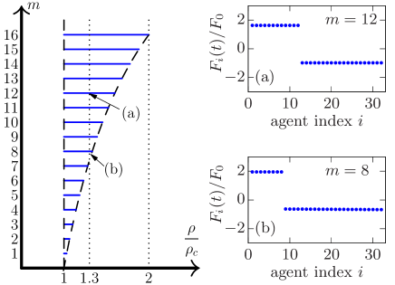
Figure 4: (Left) Phase diagram ($\rho$ vs $m$) of two-level stable solutions. The total number of the agents is $N=32$. On the horizontal solid lines, the two-level solutions are stable. Dashed lines are theoretical prediction Eq. (25). Arrows indicate the parameter values used in the right figures. (Right) Examples of asymmetric two-level solutions obtained by numerical simulations. The density $\rho$ is set as $\rho/\rho_{c}=1.3$. The number of the upper-level agents $m$ is (a) $m=12$, and (b) $m=8$. A weakly hierarchical state $F_{i}(0)$, similar to the one shown in Fig. 2(a), is used as the initial condition, which is sorted as $F_{i}(0)>F_{j}(0)$ for $i<j$. Note that this order of $F_{i}(t)$ does not change with $t$ in the mean-field model [i.e., $i_{\alpha}(t)\equiv\alpha$], thus the agent index $i$ is used as the horizontal axis.

Linear stability analysis can be carried out in the same way as the previous subsection. The Jacobian at the two-level steady solutions is given by

$$J_{2,m}=\begin{pmatrix}J_{1,m}(a)&O\\ O&J_{1,N-m}(a^{\prime})\end{pmatrix},$$ (23)

where $J_{1,m}(a)$ is an $m\times m$ matrix of the form of Eq. (15) but with $a=\rho(m-1)/(2N^{\prime})-1$ [$b$ is the same as that in Eq. (15)], $J_{1,N-m}(a^{\prime})$ is an $(N-m)\times(N-m)$ matrix with $a^{\prime}=\rho(N-m-1)/(2N^{\prime})-1$, and $O$ is a zero matrix. By using Eq. (16), it is easy to find the eigenvalues of $J_{2,m}$ as

$$\lambda=-1,\,\,\rho\frac{m}{2N^{\prime}}-1,\,\,\rho\frac{N-m}{2N^{\prime}}-1,$$ (24)

with multiplicities $2,m-1$, and $N-m-1$, respectively. Therefore, the two-level stable solution with $m$ exists for $\rho$ satisfying

$$1<\frac{\rho}{\rho_{c}}<\frac{N}{N-m}.$$ (25)

Thus, at $\rho=\rho_{c}$, the steady solution of Eq. (14) changes abruptly from $F_{i}(t)\equiv 0$ to the above values in Eq. (22). This discontinuity originates from the fact that $f(x)$ is not differentiable. Even for $\rho/\rho_{c}>N/(N-m)$, the two-level solutions with $m$ exist, but they are unstable because the third eigenvalue in Eq. (24) becomes positive.

In Fig. 4, the ranges of $\rho$ where a stable two-level solution exists are displayed by horizontal lines. The symmetric solution ($m=N/2$) has the widest stable range; the stable range is shorter for stronger asymmetry (i.e., for smaller values of $m$). Asymmetric solutions shown in Figs. 4 (a) and (b) are obtained by numerical simulations; these solutions resemble the result for the agent model shown in Fig. 2(b).

As shown in Fig. 4(Left), the two-level solutions ($m=1,\dots,N-1$) appear simultaneously at $\rho=\rho_{c}$ through bifurcations of the pitchfork type (though there is a discontinuity). This can be easily checked by setting $F_{i}(t)=F^{u}(t)$ for ($i\leq m$), and $F_{i}(t)=-F^{l}(t)$ for ($i>m$); this form of the trajectory $F_{i}(t)$ is a solution in an invariant two-dimensional subspace. If we define $\Delta F(t)=F^{u}(t)+F^{l}(t)$, it is easy to show that

$$\frac{d\Delta F(t)}{dt}=-\Delta F(t)+\frac{2\rho}{\rho_{c}}f\bigl{(}\Delta F(t)\bigr{)}.$$ (26)

Examining the functional form of the right side [as a function of $\Delta F(t)$] for $\rho<\rho_{c}$ and $\rho>\rho_{c}$, it is found that the bifurcation at $\rho=\rho_{c}$ is the superciritical pitchfork type Strogatz (1994). Note however that this analysis in invariant subspaces is insufficient for a proof of the linear stability. See Appendix B for a similar argument on three-level solutions, for which two stable solutions appear also through the superciritical pitchfork bifurcations, but they are unstable in some directions perpendicular to the invariant subspaces.

III.3 Three-level solution

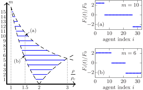
Figure 5: (Left) Phase diagram ($\rho$ vs $m$) of three-level stable solutions. The total number of the agents is $N=32$. On the horizontal solid lines, the three-level solutions are stable. Dashed lines are theoretical prediction Eq. (31). Arrows indicate the parameter values used in the right figures. (Right) Examples of three-level solutions obtained by numerical simulations. The density $\rho$ is set as $\rho/\rho_{c}=1.5$. Half the number of the middle-level agents $m$ is (a) $m=10$, and (b) $m=6$. Weakly hierarchical states, similar to the one shown in Fig. 3(a), are used as initial conditions.

There are also many three-level steady solutions, and thus here we focus only on symmetric three-level solutions. In this subsection, steady solutions of the following form are shown to be stable:

$$F_{i}(t)\equiv\begin{cases}F&\left(1\leq i\leq\frac{N}{2}-m\right),\\[2.84544pt] 0&\left(\frac{N}{2}-m<i\leq\frac{N}{2}+m\right),\\[2.84544pt] -F&\left(\frac{N}{2}+m<i\leq N\right).\end{cases}$$ (27)

Here, $2m$ is the number of the middle-level agents, for which $F_{i}(t)\equiv 0$; therefore $m$ should satisfy $0<m<N/2$. Moreover, the constant $F$ is assumed to satisfy $F>2$ (even if $F<2$, there exist some steady solutions, but they are linearly unstable. See Appendix B). Substituting Eq. (27) into the right side of Eq. (14), we found that

$$F=\frac{\rho}{\rho_{c}}+\frac{\rho m}{N^{\prime}}.$$ (28)

Since we assume $F>2$, the steady solution [Eq. (28)] exists for $\rho>4N^{\prime}/(N+2m)$.

The Jacobian of these steady solutions is given by

$$J_{3,m}^{F>2}=\begin{pmatrix}J_{1,N/2-m}(a)&O&O\\[5.69046pt] O&J_{1,2m}(a^{\prime})&O\\[5.69046pt] O&O&J_{1,N/2-m}(a)\end{pmatrix},$$ (29)

where $J_{1,N/2-m}(a)$ is an $(N/2-m)\times(N/2-m)$ matrix of the form of Eq. (15) with $a=\rho(N^{\prime}-1-2m)/(4N^{\prime})-1$, and $J_{1,m}(a^{\prime})$ is an $2m\times 2m$ matrix with $a=\rho(2m-1)/(2N^{\prime})-1$. By using Eq. (16), we obtain the eigenvalues of $J_{3,m}^{F>2}$ as

$$\lambda=-1,\,\,\rho\frac{N-2m}{4N^{\prime}}-1,\,\,\rho\frac{m}{N^{\prime}}-1,$$ (30)

with multiplicities $3,N-2m-2$, and $2m-1$, respectively. Therefore, the three-level stable solution with $m$ [Eq. (27)] exists for $\rho$ satisfying

$$\frac{2N}{N+2m}<\frac{\rho}{\rho_{c}}<\mathrm{max}\left(\frac{2N}{N-2m},\,\,\frac{N}{2m}\right).$$ (31)

Even for $\rho/\rho_{c}$ larger than this upper bound, the three-level solutions exist, but they are unstable because the second or the third eigenvalues in Eq. (30) become positive.

In Fig. 5, the ranges of $\rho$ where the stable three-level solutions exist are displayed by horizontal lines. The widest stable range is at $m=N/6$, at which the three levels have the equal numbers of agents (the example shown in the figure is for $N=32$, and thus $N/6$ is not an integer. If $N$ is a multiple of $3$, there is a steady solution for which each level has $N/3$ agents). In Figs. 5 (a) and (b), solutions obtained by numerical simulations are displayed. These solutions resemble the result for the agent model shown in Fig. 3(b).

III.4 $N$-level solution (linear hierarchy)

Linear hierarchies are frequently observed in animal societies. In a linear hierarchy, if an individual A dominates B and B dominates C, then A dominates C Chase et al. (2002) (i.e., a transitive relationship). At high values of $\rho$, there exists a steady $N$-level solution, in which each agent has a different values of $F_{i}(t)$. This completely stratified solution is reminiscent of the linear hierarchy.

Here, let us assume the following solution

$$F_{i}(t)\equiv F-\frac{2F}{N^{\prime}}(i-1),\quad(i=1,\dots,N),$$ (32)

where $F$ is a constant to be determined, and we also assume $F>N^{\prime}$. In order that the above $F_{i}(t)$ is a steady solution, i.e., $dF_{i}(t)/dt\equiv 0$ in Eq. (14), $F$ should satisfy

$$F=\rho.$$ (33)

In the derivation, we used the assumption $F>N^{\prime}$ as $F_{i}(t)-F_{j}(t)=2F(j-i)/N^{\prime}>2F/N^{\prime}>2$, where $i<j$. From $F>N^{\prime}$ and Eq. (33), $\rho$ should also satisfy $\rho>N^{\prime}$, or

$$\frac{\rho}{\rho_{c}}>\frac{N}{2}.$$ (34)

Thus, the $N$-level solution exists only at large $\rho$.

The stability of the $N$-level solution is easy to prove. The Jacobian of this steady solution is simply given by $J_{N}=-I$, where $I$ is the $N\times N$ identity matrix. Therefore, the $N$-level solution [Eq. (32)] is stable.

IV Ergodicity in agent model

As shown in Figs. 2 and 3, the agent model behaves similarly to the mean-field model for $1/\gamma\ll T_{0}$ and $\eta\ll F_{0}$. But, if these conditions are not fulfilled, the agent model behaves differently from the mean-field model. In this section, the dependence of the agent model on these parameters $\gamma$ and $\eta$ is numerically studied.

As a quantity characterizing the dynamics of the agent model, we use the standard deviation $\sigma(\gamma,\eta)$ of the time-averaged DS, $\overline{F}_{i}$, defined as

$$\mu(\gamma,\eta) :=\frac{1}{N}\sum_{i=1}^{N}\overline{F}_{i},$$ (35)

$$\sigma^{2}(\gamma,\eta) :=\frac{1}{N}\sum_{i=1}^{N}[\overline{F}_{i}-\mu(\gamma,\eta)]^{2}.$$ (36)

The time averaged DS, $\overline{F}_{i}$, is defined as

$$\overline{F}_{i}:=\frac{1}{T}\int_{0}^{T}F_{i}(t)dt,$$ (37)

where the dynamics of $F_{i}(t)$ is given by Eq. (1) with the parameters $\eta$ and $\gamma$. Thus, the standard deviation $\sigma(\gamma,\eta)$ also depends on these parameters.

If the system is ergodic, a time average tends to a single value, which is equal to the ensemble average, in a long time limit ($T\to\infty$). In the agent model [Eqs. (1) and (2)], all the agents are equivalent, and therefore the limiting value is the same for all the agents, and thus it follows that $\sigma(\gamma,\eta)$ vanishes at $T\to\infty$. Accordingly, $\sigma(\gamma,\eta)$ can be used as a parameter of ergodicity breaking He et al. (2008); Miyaguchi and Akimoto (2013). In Fig. 6, we set $\gamma\eta$ is constant (i.e., $\rho=\gamma\eta$ is constant) to fix the corresponding mean-field model [See Eq. (13)], and numerically obtain the variance $\sigma^{2}(\rho/\eta,\eta)$ as a function of $\eta$.

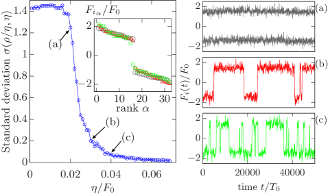
Figure 6: (Left) Standard deviation $\sigma(\rho/\eta,\eta)$ vs $\eta$ in the agent model with $N=32$. The value of $\rho$ is fixed as $\rho=1.5\rho_{c}$, for which the egalitarian solution $F_{i}(t)\equiv 0$ is unstable in the mean-field approximation. Arrows indicate the parameter values used in the right figures. The time average in Eq. (37) is taken over a time interval during which $10^{9}$ contests occur. The inset is a snapshot of $F_{i_{\alpha}}(t)$ vs rank $\alpha$ for $\eta=0.02F_{0}$ (circle), $\eta=0.03F_{0}$ (triangle), and $\eta=0.04F_{0}$ (square). (Right) Typical trajectories of $F_{i}(t)$ for (a) $\eta=0.02F_{0}$, (b) $\eta=0.03F_{0}$, and (c) $\eta=0.04F_{0}$. In (a), two trajectories are displayed, whereas a single trajectory is displayed in (b) and (c).

As shown in Fig. 6 (Left), the standard deviation $\sigma(\rho/\eta,\eta)$ is far away from zero for small values of $\eta$. In fact, the agents are separated into two groups as shown in the inset of Fig. 6(Left); these two groups correspond to the two-level solution in the mean-field model with $m=N/2$ [Eq. (20)]. For small $\eta$, the members of these two groups rarely change in the course of time evolution, as shown in Fig. 6(a), where two typical trajectories $F_{i}(t)$ are displayed.

For large values of $\eta$, the agents are still separated into two groups again [See the inset of Fig. 6(Left)], but the agents frequently move from one group to the other as shown in Figs. 6(b) and (c). Accordingly, all the time averages $\overline{F}_{i}$ ($i=1,\dots,N$) tend to zero as $T$ increases, and therefore the standard deviation $\sigma(\rho/\eta,\eta)$ also vanishes as shown in Fig. 6 (Left). The transitions of the agents from one group to the other occur, because the impact of each contest becomes significant for large $\eta$ [though a time average of this effect, given by $\gamma\eta$, is the same in all the numerical simulations in Figs. 6 (a)–(c)]. It should be also noted that, even though the time average $\overline{F}_{i}$ vanishes at large $\eta$, a hierarchy exists in snapshots $F_{i}(t)$ as shown in the inset of Fig. 6(Left), where the agents are separated into two groups, and thus the system is not egalitarian.

At small $\eta$, the ergodicity seems to be violated as shown in Fig. 6(a). However, it is probable that it just takes too long time to observe transitions of the agents from one group to the other, and thus the ergodicity might not be violated. This is because a sequence of contests at large $\eta$ which causes a transition of an agent can be possible, in principle, to occur even at small $\eta$ (though the probability of occurrence of such sequence of contests is quite small). Therefore, the observed violation of the ergodicity might well be just apparent.

V Discussion

Since the appearance of the seminal paper Bonabeau et al. (1995), the Bonabeau model has been employed to explain experimental data of animal hierarchy formations, and many modified versions have been proposed Stauffer (2003); Stauffer and Sa Martins (2003); Odagaki and Tsujiguchi (2006); Okubo and Odagaki (2007); Tsujiguchi and Odagaki (2007). But, understanding of the original Bonabeau model has not been far from satisfactory due to difficulty in treating its nonlinearity. In this paper, a piecewise linear version of the Bonabeau model was introduced. By using the mean-field approximation, it was shown that there are many asymmetric solutions, and that coexistence of the stable solutions takes place. In addition, an apparent transition in ergodic behaviors is found in the agent model.

Our model assumed that encounters of the agents are completely random. Namely, at each contest time $t_{n}$, the agents $i$ and $j$ are randomly chosen from the $N$ agents. But, it is known that if the agents $i$ and $j$ contest, then these agents $i$ and $j$ are more likely to contest in the next contest event than other agents Lindquist and Chase (2009). Remarkably, it is also shown in Ref. Lindquist and Chase (2009) that the persistent time during which the same individuals successively contest follows a power-law distribution. Such a non-Markovian memory effect can be easily implemented in the agent model, by introducing a persistent-time distribution Miyaguchi and Akimoto (2013); Miyaguchi et al. (2019)

$$w_{\mathrm{p}}(\tilde{\tau})\simeq\frac{a}{\tilde{\tau}^{1+\alpha}}\quad(\tau\to\infty),$$ (38)

where $a$ and $\alpha$ are positive constants. We choose a sequences of persistent times $\tilde{\tau}_{1},\tilde{\tau}_{2},\cdots$, each following $w_{\mathrm{p}}(\tilde{\tau})$, and define renewal times as $\tilde{t}_{n}:=\sum_{k=1}^{n}\tilde{\tau}_{k}$, at which the contestants change. In each interval $[\tilde{t}_{n-1},\tilde{t}_{n}]$, the same agents $i$ and $j$ contest. This generalized model should be studied in future works.

The linear hierarchy, frequently observed in animal societies, is characterized by the transitive relationship (See Sec. III.4); however, intransitive relationships are also observed by suppressing group processes Chase et al. (2002). Such intransitive relationships cannot be described by the Bonabeau model, because it is always transitive from its definition; i.e., if $F_{i}(t)>F_{j}(t)$ and $F_{j}(t)>F_{k}(t)$, then $F_{i}(t)>F_{k}(t)$. To describe the intransitive relationships, it is necessary to introduce an anti-symmetric matrix $F_{ij}(t)$ which describes the dominance relationship between $i$ and $j$. In the Bonabeau model, $F_{ij}(t)$ could be defined by $F_{ij}(t):=F_{i}(t)-F_{j}(t)$, but the matrix $F_{ij}(t)$ cannot be described by a single vector in general.

Therefore, future work is needed to develop a generalized model for $F_{ij}(t)$, and to elucidate how the transitive relationship [i.e., if $F_{ij}(t)>0$ and $F_{jk}(t)>0$, then $F_{ik}(t)>0$] emerges (or self-organizes). In such a generalized model, a bystander effect should be incorporated, in addition to the winner/loser effects Chase et al. (2002); Grosenick et al. (2007). The bystander effect is a mechanism that an individual who witnesses a contest between other individuals is influenced by the result of that contest; the witness might learn its status vicariously by observing contests between other individuals Grosenick et al. (2007). Without such a bystander effect, intransitive relationships should be frequently observed Chase et al. (2002).

Finally, we neglect the noise terms in Eqs. (1) and (2) in this paper, and thus contest dynamics is purely deterministic except the random choice of two contestants. In real societies, however, contestants have some random factors such as their physical conditions. Therefore, the noise terms might be important and should be studied in future works.

Appendix A Rescaling

In this Appendix, the agent model and the mean-field-model are transformed into simpler forms by introducing rescaled variables. Let us define the rescaled (non-dimensional) variables as

$$\bar{t}=\frac{t}{T_{0}},\quad\bar{F}_{i}(\bar{t})=\frac{F_{i}(t)}{F_{0}}.$$ (39)

Then, Eqs. (1) and (2) can be rewritten as (we omit the noise terms)

$$\bar{F}_{i}(\bar{t}_{n}^{+}) =\bar{F}_{i}(\bar{t}_{n}^{-})+\bar{\eta}\bar{f}(\bar{F}_{i}(\bar{t}^{-}_{n})-\bar{F}_{j}(\bar{t}^{-}_{n})),$$ (40)

$$\bar{F}_{j}(\bar{t}_{n}^{+}) =\bar{F}_{j}(\bar{t}_{n}^{-})+\bar{\eta}\bar{f}(\bar{F}_{j}(\bar{t}^{-}_{n})-\bar{F}_{i}(\bar{t}^{-}_{n})),$$ (41)

where $\bar{\eta}$ and $\bar{f}(x)$ are defined respectively as $\bar{\eta}=\eta/F_{0}$ and

$$\bar{f}(x)=\begin{cases}-1&(x<-2),\\[2.84544pt] \frac{x}{2}&(-2\leq x\leq 2),\\[2.84544pt] 1&(x>2).\end{cases}$$ (42)

The exponential distribution of the intervals $\tau$ [Eq. (10)] is also rescaled as

$$\bar{w}(\bar{\tau})=\bar{\gamma}_{a}e^{-\bar{\gamma}_{a}\bar{\tau}},$$ (43)

where $\bar{\gamma}_{a}=\gamma_{a}T_{0}$. The relaxation dynamics [Eq. (11)] is simply given by

$$\frac{d\bar{F}_{i}(\bar{t})}{d\bar{t}}=-\bar{F}_{i}(\bar{t}).$$ (44)

Therefore, the two parameters $\bar{\eta}$ and $\bar{\gamma}_{a}$ completely characterize the agent model.

Similarly, by using the transformations in Eq. (39), the mean-field model in Eq. (13) becomes

$$\frac{d\bar{F}_{i}(\bar{t})}{d\bar{t}}=\frac{\bar{\rho}}{N^{\prime}}\sum_{\begin{subarray}{c}j=1\\ j\neq i\end{subarray}}^{N}\bar{f}\bigl{(}\bar{F}_{i}(\bar{t})-\bar{F}_{j}(\bar{t})\bigr{)}-\bar{F}_{i}(\bar{t}).$$ (45)

where $\bar{\rho}$ is defined as $\bar{\rho}=\rho T_{0}/F_{0}$. Thus, $\bar{\rho}$ is the only parameter of the mean-field model. Note that, even if $\bar{\rho}$ is constant, corresponding parameter values in the agent model ($\bar{\eta}$ and $\bar{\gamma}_{a}$) are not uniquely determined, because $\bar{\rho}=\bar{\gamma}\bar{\eta}$ with $\bar{\gamma}:=2\bar{\gamma}_{a}/N$.

Appendix B Unstable three-level solution

In Sec. III.3, we study stable three-level solutions [Eq. (27)], but there also exist unstable three-level solutions. In this Appendix, we show that the three-level unstable solutions emerge simultaneously at $\rho=\rho_{c}$, and these unstable solutions become stable at some values of $\rho>\rho_{c}$.

First, it is easy to show that a steady three-level solution of the form of Eq. (27) does not exist for $0<F<1$, and we already study the three-level solutions for $F>2$ in Sec. III.3. Thus, here we assume $1<F<2$. For $1<F<2$, the three-level solution is given by

$$F=\frac{\rho}{2}\frac{N-2m}{N^{\prime}-\rho m},$$ (46)

with $m=0,\dots,N/2-1$ ($m=0$ corresponds to the symmetric two-level solution). Accordingly, the range of $\rho$ satisfying $1<F<2$ is given by

$$1<\frac{\rho}{\rho_{c}}<\frac{2N}{N+2m}.$$ (47)

Note that the upper bound is equivalent to the lower bound of the stable three-level solution [Eq. (31)]. In fact, the stability of the three-level solutions for each value of $m$ changes at $\rho/\rho_{c}=2N/(N+2m)$ as shown below. The bifurcation at this point might be subcritical-pitchfork type (however, we should note that details of this bifurcation remain still unclear).

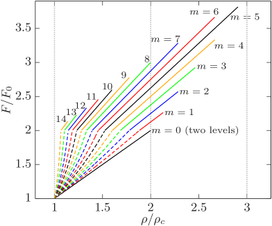
Figure 7: Dominance score $F$ for two-level and three-level symmetric solutions as functions of $\rho$. The number of agents are set as $N=32$. The numbers in the figure are the corresponding values of $m$. The dashed curves are unstable solutions given by Eq. (46), and the solid curves are stable two-level and three level solutions given by Eq. (22) with $m=N/2$ and Eq. (28), respectively. Beyond these stable ranges, all the solutions with $m$ still exist, but they are unstable (See Secs. III.2 and III.3). These unstable ranges are not shown for brevity.

Next, the stability of the three-level solutions [Eq. (46)] is elucidated. In this case, the Jacobian matrix is given by

$$J_{3,m}^{1<F<2}=\begin{pmatrix}J_{1,N/2-m}(a)&B&O\\[5.69046pt] B^{t}&J_{1,2m}(a^{\prime})&B^{t}\\[5.69046pt] O&B&J_{1,N/2-m}(a)\end{pmatrix},$$ (48)

where $J_{1,N/2-m}$ is an $(N/2-m)\times(N/2-m)$ matrix of the form of Eq. (15) with $a=\rho(N^{\prime}+2m-1)/(4N^{\prime})-1$, $J_{1,2m}(a^{\prime})$ is a $2m\times 2m$ matrix with $a^{\prime}=\rho/2-1$, and $B$ is an $(N/2-m)\times 2m$ matrix, all the elements of which are the same and given by $-\rho/(2N^{\prime})$. $B^{t}$ is the transpose of $B$.

After a somewhat lengthy but elementary calculation, we obtain four eigenvalues of the Jacobian in Eq. (48). Two of the four eigenvalues are given by

$$\lambda=\frac{\rho}{\rho_{c}}-1,\quad\rho\frac{N+2m}{4N^{\prime}}-1,$$ (49)

with multiplicities $2m$ and $N-2(m+1)$, respectively. The first eigenvalue in Eq. (49) is positive because of Eq. (47). Therefore, the three-level solutions in Eq. (46) are unstable. Note however that the first eigenvalue does not exist for $m=0$ (i.e., for the two-level symmetric solution), because the multiplicity becomes zero, and therefore it is not contradicting with the fact that the two-level solution is stable (See Sec. III.2). Note also that the second eigenvalue is negative, and it does not exist, if $m=N/2-1$. The remaining two eigenvalues are given by

$$\lambda=-1,\quad\rho\frac{m}{N^{\prime}}-1.$$ (50)

These eigenvalues are simple and negative.

A phase diagram of the symmetric two- and three-level solutions are displayed in Fig. 7. These steady solutions emerge at $\rho=\rho_{c}$, but only two-level solution is stable, and all the three-level solutions are unstable. For $F>2$, however, the two-level solution becomes unstable (See Sec. III.2), whereas the three-level solutions, which are given by Eq. (28), become stable.

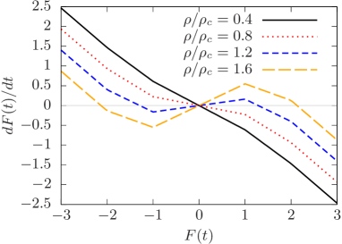
Figure 8: $dF(t)/dt$ in Eq. (52) vs $F(t)$ for four different values of $\rho$: $\rho/\rho_{c}=0.4$ (solid line), $0.8$ (dotted line), $1.2$ (dashed line), and $1.6$ (long-dashed line). $N$ and $m$ are set as $N=32$ and $m=6$. For $\rho<\rho_{c}$, $dF(t)/dt$ is monotonically decreasing, and thus the origin $F(t)\equiv 0$ is the stable fixed point. For $\rho>\rho_{c}$, however, the origin is unstable, and two stable fixed points, that correspond to Eq. (46), appear. Note that these stable fixed points are stable only in the invariant subspace, and unstable in some directions perpendicular to this subspace.

Finally, let us consider how these solutions emerge. To elucidate this, we study one-dimensional invariant subspaces described by the following solution

$$F_{i}(t)=\begin{cases}F(t)&\left(1\leq i\leq\frac{N}{2}-m\right),\\[2.84544pt] 0&\left(\frac{N}{2}-m<i\leq\frac{N}{2}+m\right),\\[2.84544pt] -F(t)&\left(\frac{N}{2}+m<i\leq N\right),\end{cases}$$ (51)

where $m=0,1,\dots,N/2-1$, and $F(t)$ can be either positive or negative. The time evolution equation for $F(t)$ is obtained by inserting Eq. (51) into Eq. (14) as

$$\frac{dF(t)}{dt} =-F(t)+\frac{\rho}{N^{\prime}}\left[2mf\bigl{(}F(t)\bigr{)}+\frac{N-2m}{2}f\bigl{(}2F(t)\bigr{)}\right]$$

$$=\begin{cases}\left(\frac{\rho}{\rho_{c}}-1\right)F(t)&[0<F(t)<1],\\[5.69046pt] \left(\rho\frac{m}{N^{\prime}}-1\right)F(t)+\rho\frac{N-2m}{2N^{\prime}}&[1<F(t)<2],\\[5.69046pt] -F(t)+\rho\frac{N+2m}{2N^{\prime}}&[2<F(t)],\end{cases}$$ (52)

where the equation only for $F(t)>0$ is explicitly given; the explicit expression for $F(t)<0$ is readily obtained from the fact that $f(x)$ given in Eq. (42) is an odd function. Note also that the slope $\rho m/N^{\prime}-1$ in Eq. (52), which is negative for $\rho>\rho_{c}$, corresponds to the second eigenvalue in Eq. (50).

From the first equation in the right side of Eq. (52), the single-level solution $F(t)\equiv 0$ is stable for $\rho<\rho_{c}$ and unstable for $\rho>\rho_{c}$. The two-level ($m=0$) and three-level ($m>0$) solutions emerge at $\rho=\rho_{c}$ simultaneously, and they are stable because of $\rho m/N^{\prime}-1<0$ for $\rho>\rho_{c}$. Due to the symmetry, $-F(t)$ is also a solution in the invariant subspaces, and thus there are two stable fixed points in each invariant subspace with $m$.

This bifurcation is readily understood by a phase diagram Strogatz (1994) shown in Fig. 8, in which $dF(t)/dt$ in Eq. (52) is displayed as a function of $F(t)$. It is clear that the bifurcation at $\rho=\rho_{c}$ can be considered as a superciritical pitchfork type. Although the bifurcations are pitchfork type and thus the two emerged fixed points are stable, these fixed points except the two-level solutions ($m=0$) are stable only in the invariant subspaces; in fact, they are unstable in some directions perpendicular to the subspaces, because the first eigenvalue in Eq. (49) is positive.

References

- Oliveira and Holldobler (1990) P. S. Oliveira and B. Holldobler, Behav. Ecol. Sociobiol. 27, 385 (1990).
- Goessmann et al. (2000) C. Goessmann, C. Hemelrijk, and R. Huber, Behav. Ecol. Sociobiol. 48, 418 (2000).
- Chase et al. (2002) I. D. Chase, C. Tovey, D. Spangler-Martin, and M. Manfredonia, Proc. Natl. Acad. Sci. U.S.A 99, 5744 (2002).
- Grosenick et al. (2007) L. Grosenick, T. S. Clement, and R. D. Fernald, Nature 445, 429 (2007).
- Lindquist and Chase (2009) W. B. Lindquist and I. D. Chase, Bulletin of mathematical biology 71, 556 (2009).
- Wittig and Boesch (2003) R. M. Wittig and C. Boesch, Int. J. Primatology 24, 847 (2003).
- Savin-Williams (1980) R. C. Savin-Williams, J. Youth Adolescence 9, 75 (1980).
- Garandeau et al. (2014) C. Garandeau, I. Lee, and C. Salmivalli, J. Youth Adolescence 43, 1123 (2014).
- Castellano et al. (2009) C. Castellano, S. Fortunato, and V. Loreto, Rev. Mod. Phys. 81, 591 (2009).
- Hsu et al. (2006) Y. Hsu, R. L. Earley, and L. L. Wolf, Biol. Rev. 81, 33 (2006).
- Bonabeau et al. (1995) E. Bonabeau, G. Theraulaz, and J.-L. Deneubourg, Physica A 217, 373 (1995).
- Bonabeau et al. (1999) E. Bonabeau, G. Theraulaz, and J.-L. Deneubourg, Bulletin of mathematical biology 61, 727 (1999).
- Stauffer (2003) D. Stauffer, Int. J. Mod. Phys. C 14, 237 (2003).
- Stauffer and Sa Martins (2003) D. Stauffer and J. Sa Martins, Advances in Complex Systems 06, 559 (2003).
- Lacasa and Luque (2006) L. Lacasa and B. Luque, Physica A: Statistical Mechanics and its Applications 366, 472 (2006).
- (16) M. Pósfai and R. M. D’Souza, Phys. Rev. E 98, 020302.
- Odagaki and Tsujiguchi (2006) T. Odagaki and M. Tsujiguchi, Physica A 367, 435 (2006).
- Tsujiguchi and Odagaki (2007) M. Tsujiguchi and T. Odagaki, Physica A 375, 317 (2007).
- Okubo and Odagaki (2007) T. Okubo and T. Odagaki, Phys. Rev. E 76, 036105 (2007).
- Ben-Naim and Redner (2005) E. Ben-Naim and S. Redner, J. Stat. Mech. 2005, L11002 (2005).
- Ben-Naim et al. (2006) E. Ben-Naim, F. Vazquez, and S. Redner, Euro. Phys. J. B 49, 531 (2006).
- Ben-Naim et al. (2007) E. Ben-Naim, S. Redner, and F. Vazquez, Europhys. Lett. 77, 30005 (2007).
- Devaney (1984) R. L. Devaney, Physica D 10, 387 (1984).
- Tasaki and Gaspard (2002) S. Tasaki and P. Gaspard, J. Stat. Phys. 109, 803 (2002).
- Miyaguchi (2006) T. Miyaguchi, Prog. Theore. Phys. 115, 31 (2006).
- Miyaguchi and Aizawa (2007) T. Miyaguchi and Y. Aizawa, Phys. Rev. E 75, 066201 (2007).
- Strogatz (1994) S. Strogatz, Nonlinear dynamics and chaos: with applications to physics, biology, chemistry, and engineering (Westview Press, Cambridge, MA, 1994).
- Feller (1971) W. Feller, An Introduction to Probability Theory and its Applications, 2nd ed., Vol. II (Wiley, New York, 1971).
- Note (1) More precisely, should be satisfied. If we can choose satisfying this condition with , the approximation in Eq. (12) is valid.
- He et al. (2008) Y. He, S. Burov, R. Metzler, and E. Barkai, Phys. Rev. Lett. 101, 058101 (2008).
- Miyaguchi and Akimoto (2013) T. Miyaguchi and T. Akimoto, Phys. Rev. E 87, 032130 (2013).
- Miyaguchi et al. (2019) T. Miyaguchi, T. Uneyama, and T. Akimoto, Phys. Rev. E 100, 012116 (2019).