Barycentric cuts through a convex body

Abstract

Let $K$ be a convex body in $\mathbb{R}^{n}$ (i.e., a compact convex set with nonempty interior). Given a point $p$ in the interior of $K$, a hyperplane $h$ passing through $p$ is called barycentric if $p$ is the barycenter of $K\cap h$. In 1961, Grünbaum raised the question whether, for every $K$, there exists an interior point $p$ through which there are at least $n+1$ distinct barycentric hyperplanes. Two years later, this was seemingly resolved affirmatively by showing that this is the case if $p=p_{0}$ is the point of maximal depth in $K$. However, while working on a related question, we noticed that one of the auxiliary claims in the proof is incorrect. Here, we provide a counterexample; this re-opens Grünbaum’s question.

It follows from known results that for $n\geq 2$, there are always at least three distinct barycentric cuts through the point $p_{0}\in K$ of maximal depth. Using tools related to Morse theory we are able to improve this bound: four distinct barycentric cuts through $p_{0}$ are guaranteed if $n\geq 3$.

1 Introduction

Grünbaum’s questions.

Let $K$ be a convex body in $\mathbb{R}^{n}$ (i.e., compact convex set with nonempty interior). Given an interior point $p\in K$, a hyperplane $h$ passing through $p$ is called barycentric if $p$ is the barycenter (also known as the centroid) of the intersection $K\cap h$. In 1961, Grünbaum [Grü61] raised the following questions (see also [Grü63, §6.1.4]):

Question 1.

Does there always exist an interior point $p\in K$ through which there are at least $n+1$ distinct barycentric hyperplanes?

Question 2.

In particular, is this true if $p$ is the barycenter of $K$?

Seemingly, Question 1 was answered affirmatively by Grünbaum himself [Grü63, §6.2] two years later, by using a variant of Helly’s theorem to show that there are at least $n+1$ barycentric cuts through the point of $K$ of maximal depth (we will recall the definition below). The assertion that Question 1 is resolved has also been reiterated in other geometric literature [CFG94, A8]. However, when working on Question 2, which remains open, we identified a concrete problem in Grünbaum’s argument for the affirmative answer for the point of the maximal depth. The first aim of this paper is to point out this problem, which re-opens Question 1.

Depth, depth-realizing hyperplanes, and the point of maximum depth.

In order to describe the problem with Grünbaum’s argument, we need a few definitions. Let $p$ be a point in $K$. For a unit vector $v$ in the unit sphere $S^{n-1}\subseteq\mathbb{R}^{n}$, let $h_{v}=h_{v}^{p}:=\{x\in\mathbb{R}^{n}\colon\langle v,x-p\rangle=0\}$ be the hyperplane orthogonal to $v$ and passing through $p$, and let $H_{v}=H_{v}^{p}:=\{x\in\mathbb{R}^{n}\colon\langle v,x-p\rangle\geq 0\}$ be the half-space bounded by $h_{v}$ in the direction of $v$. Given $p$, we define the depth function $\delta^{p}\colon S^{n-1}\to[0,1]$ via $\delta^{p}(v)=\lambda(H_{v}\cap K)/\lambda(K)$, where $\lambda$ is the Lebesgue measure ($n$-dimensional volume) in $\mathbb{R}^{n}$. The depth of a point $p$ in $K$ is defined as $\operatorname{depth}(p,K):=\inf_{v\in S^{n-1}}\delta^{p}(v).$ It is easy to see that $\delta^{p}$ is a continuous function, therefore the infimum in the definition is attained at some $v\in S^{n-1}$. Any hyperplane $h_{v}$ through $p$ such that $\operatorname{depth}(p,K)=\delta^{p}(v)$ is said to realize the depth of $p$. Finally, a point of maximal depth in $K$ is a point $p_{0}$ in the interior of $K$ such that $\operatorname{depth}(p_{0},K):=\max\operatorname{depth}(p,K)$ where the maximum is taken over all points in the interior of $K$. The point of maximal depth always exists (by compactness of $S^{n-1}$) and it is unique (two such points would yield a point of larger depth on the segment between them).

Many depth-realizing hyperplanes?

Grünbaum’s argument has two ingredients. The first is the following result, known as Dupin’s theorem [Dup22], which dates back to 1822:

Theorem 3 (Dupin’s Theorem).

If a hyperplane $h$ through $p$ realizes the depth of $p$ then it is barycentric with respect to $p$.

Grünbaum refers to Blaschke [Bla17] for a proof; for a more recent reference, see [SW94, Lemma 2]. A stronger statement will be the content of Proposition 11 below.

The second ingredient in Grünbaum’s argument is the following assertion (which in [Grü63, §6.2] is deduced using a variant of Helly’s theorem, without providing the details).

Postulate 4.

If $p_{0}$ is the point of $K$ of maxiumal depth, then there are at least $n+1$ distinct hyperplanes through $p_{0}$ that realize the depth.

If correct, Postulate 4, in combination with Dupin’s theorem, would immediately imply an affirmative answer to Question 1. However, it turns out that this step is problematic. Indeed, there is a counterexample to Postulate 4:

Proposition 5.

Let $K=T\times I\subseteq\mathbb{R}^{3}$ where $T$ is an equilateral triangle and $I$ is a line segment (interval) orthogonal to $T$, and let $p_{0}\in K$ be the point of maximal depth (which in this case coincides with the barycenter of $K$). Then there are only $3$ hyperplanes realizing the depth of $p_{0}$.

Remark 6.

We believe that Proposition 5 can be generalized to higher dimensions in the sense that, for every $n$, there are only $n$ depth-realizing hyperplanes through the point of maximal depth in $\Delta\times I\subseteq\mathbb{R}^{n}$, where $\Delta$ is a regular $(n-1)$-simplex. However, we did not attempt to work out the details carefully, because Kynčl and Valtr [KV19] informed us about stronger counterexamples: For every $n$, there exists a convex body $K\in\mathbb{R}^{n}$ such that there are only $3$ depth-realizing hyperplanes through the point of maximal depth in $K$. Therefore, we prefer to keep the proof of Proposition 5 as simple as possible and focus on dimension $3$.

Remark 7.

We emphasize that Proposition 5 does not preclude an affirmative answer to Grünbaum’s Question 1 (nor to Question 2), since $T\times I$ contains infinitely many distinct barycentric hyperplanes through $p_{0}$. Thus Grünbaum’s questions remain open.

We also remark that a weakening of Postulate 4 is known to be true (see the ‘Inverse Ray Basis Theorem [RR99], using the proof from [DG92]):^,

Proposition 8.

Let $U\subseteq S^{n-1}$ be the set of vectors $u$ such that $\delta^{p_{0}}(u)=\operatorname{depth}(p_{0},K)$. Then $0\in\operatorname{conv}U$.

In the special case that $U$ is in general position, the cardinality of $U$ is at least $n+1$ (otherwise $\dim\operatorname{conv}U<n$ and $\operatorname{conv}U$ would not contain the origin, by general position), which proves Postulate 4 in this special case. However, $U$ need not be always in general position. For example, in the case $K=T\times I$ in $\mathbb{R}^{3}=\mathbb{R}^{2}\times\mathbb{R}$ of Proposition 5, the set $U$ contains three vectors in the plane through the origin parallel with $T$. This is also the way we arrived at the counterexample from Proposition 5.

Inverse Ray Basis Theorem immediately implies that three barycentric hyperplanes are guaranteed in dimension at least $2$.

Corollary 9.

Let $K$ be a convex body in $\mathbb{R}^{n}$ where $n\geq 2$ and $p_{0}$ be the point of maximal depth of $K$. Then there at least three distinct barycentric hyperplanes through $p_{0}$.

Proof.

Let $U$ be the set from Proposition 8. Then, $0\in\operatorname{conv}U$ and $U\subseteq S^{n-1}$ imply together $|U|\geq 2$. However, if $|U|=2$, then $U=\{u,-u\}$ for some $u\in S^{n-1}$. This necessarily means $\operatorname{depth}(p_{0},K)=\delta^{p_{0}}(u)=\delta^{p_{0}}(-u)=1/2$ as $\delta^{p_{0}}(u)+\delta^{p_{0}}(-u)=1$. Then for any other $v\in S^{n-1}$ we get $\min\{\delta^{p_{0}}(v),\delta^{p_{0}}(-v)\}\geq 1/2$ which implies $\delta^{p_{0}}(v)=\delta^{p_{0}}(-v)=1/2$ as well. Therefore $v\in U$ contradicting $|U|=2$.) ∎

Four barycentric cuts via critical points of $C^{1}$ functions.

Using tools related to Morse theory, we are able to obtain one more barycentric hyperplane, provided that $n\geq 3$.

Theorem 10.

Let $K$ be a convex body in $\mathbb{R}^{n}$ where $n\geq 3$ and $p_{0}$ be the point of maximal depth of $K$. Then there are at least four distinct hyperplanes $h$ such that $p_{0}$ is the barycenter of $K\cap h$.

Here we should also mention related work of Blagojević and Karasev [Kar11, Theorem 3.3] and [BK16, Theorem 1.13]. They show that there are at least $\mu(n)$ barycentric hyperplanes passing through some interior point of $K$ (not necessarily the point of maximal depth), where $\mu(n):=\min_{f}\max_{p\in S^{n}}|f^{-1}(p)|$ is the minimum multiplicity of any continuous map $f\colon\mathbb{R}P^{n}\to S^{n}$ (here, $\mathbb{R}P^{n}$ is the $n$-dimensional real projective space). By calculations with Stiefel–Whitney classes, they obtain lower bounds for $\mu(n)$ that depend in a subtle (and non-monotone) way on $n$ (see [Kar11, Remark 1.3]). For example, $\mu(n)\geq\frac{n}{2}+1$ if $n=2^{\ell}-2$, but for values of $n$ of the form $n=2^{\ell}-1$ (e.g., for $n=3$) their methods only give a lower bound of $\mu(n)\geq 2$.

Our argument in the proof of Theorem 10 is, in certain sense, tight. For completeness we discuss this in Section 5.

In what follows, we view $S^{n-1}$ as a smooth manifold with its standard differential structure. A key tool in the proof of Theorem 10 is the following close connection between barycentric hyperplanes and the critical points of the depth function:

Proposition 11.

Let $K\subseteq\mathbb{R}^{n}$ be a convex body and $p$ be a point in the interior of $K$. Then the corresponding depth function $\delta^{p}\colon S^{n-1}\to\mathbb{R}$ is a $C^{1}$ function. In addition, $v\in S^{n-1}$ is a critical point of $\delta^{p}$ (that is, $D\delta^{p}(v)=0$, where $Df(v)$ denotes the total derivative of a function $f$ at $v$) if and only if $h_{v}$ is barycentric.

As mentioned earlier, Proposition 11 generalizes Dupin’s theorem. Indeed, if $h=h_{v}$ realizes the depth, then $v$ is a global minimum of $\delta^{p}$, hence $h$ is barycentric by Proposition 11.

In the proof, we closely follow computations by Hassairi and Regaieg [HR08] who stated an extension of Dupin’s theorem to absolutely continuous probability measures. As explained in [NSW19] (see Proposition 29, Example 7, and the surrounding text in [NSW19]), the extension of Dupin’s theorem does not hold in the full generality stated in [HR08], and it requires some additional assumptions. However, a careful check of the computations of Hassairi and Regiaeg [HR08] in the special case of uniform probability measures on convex bodies reveals not only Dupin’s theorem but all items of Proposition 11.

Regarding the proof of Theorem 10, the Inverse Ray Basis Theorem (Proposition 8) and Corollary 9 imply that $\delta^{p_{0}}$ has at least three global minima. This gives three barycentric hyperplanes via Proposition 11. Furthermore, we also get three maxima of $\delta$, as a maximum appears at $v$, if and only if a minimum appears at $-v$ (note that $h_{v}=h_{-v}$). However, it should not happen for a $C^{1}$ function on $S^{n-1}$ that it has only such critical points. We will show that there is at least one more critical point, which yields another barycentric hyperplane via Proposition 11. Namely, we show the following proposition.

Proposition 12.

Let $n\geq 2$ and let $f\colon S^{n}\to\mathbb{R}$ be a $C^{1}$ function. Let $m_{1},\dots,m_{k}$ be (not necessarily strict) local minima or maxima of $f$, where $k\geq 3$. Then there exists $u\in S^{n}$, different from $m_{1},\dots,m_{k}$, such that $Df(u)=0$.

This finishes the proof of Theorem 10 modulo Propositions 11 and 12. (Proposition 12 is applied with $k=6$.)

The main idea beyond the proof of Proposition 12 is that if we have at least three local minima or maxima, then we should also expect a saddle point (unless there are infinitely many local extremes). This would be an easy exercise for Morse functions (which are in particular $C^{2}$) via Morse theory (actually, the Morse inequalities would provide even more critical points). Working with $C^{1}$ functions adds a few difficulties, but all of them can be overcome.

Relation to probability and statistics.

The depth function, as we define it above is a special case of the (Tukey) depth of a probability measure in $\mathbb{R}^{d}$, a well-known notion in statistics [Tuk75, Don82, DG92]. More precisely, given a probability measure $\mathbf{P}$ on $\mathbb{R}^{d}$ and $p\in\mathbb{R}^{d}$, we can define $\operatorname{depth}(p,\mathbf{P}):=\inf_{v\in S^{n-1}}\mathbf{P}(H_{v})$. Then $\operatorname{depth}(p,K)$ is a special case of the uniform probablity measure on a convex body $K$, i.e., $\mathbf{P}(A):=\lambda(A)/\lambda(K)$ for $A$ Lebesgue-measurable. We refer to [NSW19] for an extensive recent survey making many connections between the depth function in statistics and geometric questions.

There is a vast amount of literature, both in computational geometry and statistics, devoted to computing the depth function in various settings (which is not easy in general). We refer, for example, to [RS98, Cha04, BCI⁺08, CMW13, DM16, LMM19] and the references therein. From this point of view, understanding the minimal possible number of critical points of the depth function is a quite fundamental property of the depth function. Via Proposition 11, this is essentially equivalent to Grünbaum’s questions.

Organization.

Proposition 5 is proved in Section 2; Proposition 11 is proved in Section 3; and Proposition 12 is proved in Section 4.

2 Few hyperplanes realizing the depth

In this section we prove Proposition 5, assuming Proposition 11.

Preliminaries.

Let us recall that given a bounded measurable set $Y\subseteq\mathbb{R}^{n}$ of positive measure, the barycenter of $Y$ is defined as

$$\operatorname{cen}Y=\frac{\int_{\mathbb{R}^{n}}x\chi_{Y}(x)dx}{\int_{\mathbb{R}^{n}}\chi_{Y}(x)dx}=\frac{1}{\lambda(Y)}\int_{Y}xdx$$ (1)

where $\chi_{Y}$ is the characteristic function and the integral is considered as a vector in $\mathbb{R}^{n}$.

If $Y$ splits as a disjoint union $Y=Y_{1}\sqcup\cdots\sqcup Y_{\ell}$ of sets of positive measure then

$$\operatorname{cen}Y=\frac{1}{\lambda(Y)}\left(\sum_{i=1}^{\ell}\lambda(Y_{i})\operatorname{cen}Y_{i}\right)$$ (2)

which easily follows from (1).

If $h$ is a hyperplane, and $Y\subseteq h$ has positive $(n-1)$-dimensional Lebesgue measure inside $h$, then the formula for the barycenter is analogous to (1):

$$\operatorname{cen}Y=\frac{\int_{h}x\chi_{Y}(x)d\lambda_{n-1}(x)}{\int_{h}\chi_{Y}(x)d\lambda_{n-1}(x)}=\frac{1}{\lambda_{n-1}(Y)}\int_{Y}xd\lambda_{n-1}(x)$$ (3)

where, for purpose of this formula, $\lambda_{n-1}$ denotes the $(n-1)$-dimensional Lebesgue measure on $h$.

If $h\subseteq\mathbb{R}^{n}$ is a hyperplane whose orthogonal projection $\pi(h)$ onto $\mathbb{R}^{n-1}\times\{0\}$ (the first $n-1$ coordinates) equals $\mathbb{R}^{n-1}\times\{0\}$, then $\operatorname{cen}\pi(Y)=\pi(\operatorname{cen}Y)$.

Proof of Proposition 5..

Let $T\subseteq\mathbb{R}^{2}$ be an equilateral triangle with $\operatorname{cen}(T)=0$ and $I=[-1,1]$. Then $\operatorname{cen}(K)=0$. In addition, because the point of maximal depth $p_{0}$ is unique and invariant under isometries of $K$, we get $p_{0}=0$.

We will use the following notation: $a$, $b$, $c$ are the vertices of $T$ and $\alpha$, $\beta$, and $\gamma$ are lines perpendicular to $T$ passing through $a$, $b$, and $c$ respectively.

Now let $h$ be a hyperplane passing through $0$. We want to find out whether $h$ realizes the depth. We will consider three cases:

1. $h$ is perpendicular to $T$;

2. $h$ is not perpendicular to $T$ and all intersection points of $h$ with $\alpha$, $\beta$, and $\gamma$ belong to $K$;

3. $h$ is not perpendicular to $T$ and at least one of the intersection points of $h$ with $\alpha$, $\beta$, and $\gamma$ does not belong to $K$.

In case (i), we will find three candidates for hyperplanes realizing the depth. Then we show that there is no hyperplane realizing the depth in cases (ii) and (iii), which shows that only the three candidates from case (i) may realize the depth. They realize the depth because we have at least three hyperplanes realizing the depth by the discussion in the introduction above Theorem 10.

Let us focus on case (i). This is the same as considering the lines realizing the depth in an equilateral triangle. It is easy to check and well known (see e.g. [RR99, §5.3]) that the depth of the equilateral triangle is $4/9$ and it is realized by lines parallel with the sides of the triangle. It follows that we can reach depth $4/9$ in $K$ by hyperplanes perpendicular to $T$ and parallel with the three sides of $T$, and all other hyperplanes from case (i) bound a portion of $K$ strictly larger than $4/9$ on each of their sides.

Case (ii) is very easy: It is easy to compute that each hyperplane of type (ii) splits $K$ into two parts of equal volume $1/2$.Therefore, no such hyperplane realizes the depth.

Finally, we investigate case (iii). Here we show that no hyperplane $h$ of case (iii) is barycentric. Therefore, by Theorem 3, it cannot realize the depth either.

We aim to show that $0$ is not the barycenter of $h\cap K$. Let $U$ be the orthogonal projection of $h\cap K$ to the triangle $T$. Equivalently, we want to show that $0$ is not the barycenter of $U$. We also realize that $U=T\cap S$, where $S$ is an infinite strip obtained as the orthogonal projection of $h\cap(\mathbb{R}^{2}\times I)$ to $\mathbb{R}^{2}\times\{0\}$; see Figure 1.

Let $s$ be the center line of $S$. This is the line where $h$ meets the plane of $T$. We remark that $0$ belongs to $s$ and in addition $U$ is a proper subset of $T$ (otherwise we would be in case (ii)). We again distinguish three cases:

1. none of the vertices $a,b,c$ belongs to $U$,

2. one of the vertices $a,b,c$ belongs to $U$,

3. two of the vertices $a,b,c$ belong to $U$.

In all the cases we will show $\operatorname{cen}U\neq\operatorname{cen}T$.

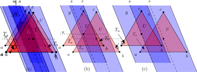
Figure 1: Three cases for the intersection $U=T\cap S$.

In case (a), $s$ splits one of the vertices of $T$ from the other two. Without loss of generality, $a$ is on one side of $s$ and $b$ and $c$ are on the other side. The center line $s$ also splits $U$ into two parts. Let $W^{\prime}$ be the (closed) part on the side of $a$, $W^{\prime\prime}$ be the mirror image of $W^{\prime}$ along $S$ and $W:=W^{\prime}\cup W^{\prime\prime}$. Note that $W$ is a proper subset of $U$; indeed, since $\operatorname{cen}T=0$ and $T$ is equilateral, the line $s$ splits the segment $ab$ closer to $b$ and the segment $ac$ closer to $c$. By the symmetry of $W$, the barycenter $\operatorname{cen}W$ belongs to the line $s$. However, this means that the barycenter of $U$ is not on $s$; it is on the $bc$ side of $s$. Formally, this follows from (2) for the decomposition $U=W\sqcup(U\setminus W)$.

In case (b), without loss of generality, $U$ contains $c$. Then $T\setminus U$ is the union of two triangles $T_{a}$ and $T_{b}$. Let $\kappa$ be the line parallel with $ab$ passing through $0$. Without loss of generality, up to rotating $T$, $\kappa$ is the $x$-axis. From (2), we get $0=\operatorname{cen}T=\frac{1}{\lambda(T)}(\lambda(U)\operatorname{cen}U+\lambda(T_{a})\operatorname{cen}T_{a}+\lambda(T_{b})\operatorname{cen}T_{b})$. The barycenters $\operatorname{cen}T_{a}$ and $\operatorname{cen}T_{b}$ are below the line $\kappa$ or on it. At least one of these barycenters is strictly below ($\operatorname{cen}T_{a}$ is on $\kappa$ if and only if $c$ belongs to the closure of $T_{a}$, and similarly with $T_{b}$). Therefore, $\operatorname{cen}U$ must be strictly above $\kappa$ if the above equality is supposed to hold.

In case (c), it is even more obvious that $\operatorname{cen}U\neq\operatorname{cen}T$. Without loss of generality $U$ contains $b$ and $c$. Then $T\setminus U$ is a triangle $T_{a}$. Since both $T$ and $T_{a}$ are convex and $T_{a}$ does not contain $\operatorname{cen}T$, we have $\operatorname{cen}T_{a}\neq\operatorname{cen}T$. Therefore $\operatorname{cen}T\neq\operatorname{cen}U$ follows from (2) for the decomposition $T=U\sqcup T_{a}$. ∎

3 Critical points of the depth function

Here we prove Proposition 11. We follow [HR08] with a slightly adjusted notation and adding a few more details here and there.

Proof of Proposition 11.

Without loss of generality, we can assume that the point $p$ coincides with the origin and we suppress it from the notation. That is, we write $\delta$ for the depth function instead of $\delta^{p}$.

Let $e_{1},\ldots,e_{n}$ be the canonical basis of $\mathbb{R}^{n}$ and let

$$S_{j+}^{n-1}=\{u=\sum_{i=1}^{n}u_{i}e_{i}\in S^{n-1};u_{j}>0\}\hskip 14.22636pt\hbox{ and }\hskip 14.22636ptS_{j-}^{n-1}=\{u=\sum_{i=1}^{n}u_{i}e_{i}\in S^{n-1};u_{j}<0\}$$

be the relatively open hemispheres of $S^{n-1}$ with poles at $e_{j}$ and $-e_{j}$, for $j\in[n]$. These sets form an atlas on $S^{n-1}$.

Let us consider $j\in[n]$. Given $x\in\mathbb{R}^{n}$ and $i\in[n]$, $x_{i}$ denotes the $i$th coordinate of $x$, that is $x=\sum_{i=1}^{n}x_{i}e_{i}$. With a slight abuse of the notation, we identify $\mathbb{R}^{n-1}$ with the subspace of $\mathbb{R}^{n}$ spanned by $e_{1},\dots,e_{j-1},e_{j+1},\dots,e_{n}$. Let $\hat{x}:=\sum_{i=1,i\neq j}^{n}x_{i}e_{i}\in\mathbb{R}^{n-1}$. Following [HR08] we consider the diffeomorphisms $u\mapsto\beta(u)=-\frac{\hat{u}}{u_{j}}$ between $S_{j+}^{n-1}$ and $\mathbb{R}^{n-1}$ or between $S_{j-}^{n-1}$ and $\mathbb{R}^{n-1}$. We will check the required properties of $\delta$ locally at each of the $2n$ hemispheres $S_{j+}^{n-1}$ or $S_{j-}^{n-1}$ (with respect to the aforementioned diffeomorphisms). Given that all cases are symmetric, it is sufficient to focus only on the $S_{n+}^{n-1}$ case. That is, from now on, we assume that $j=n$ and $\mathbb{R}^{n-1}$ is spanned by the first $(n-1)$ coordinates in the convention above. Given a point $x\in\mathbb{R}^{n}$, we also write it as $x=(\hat{x};x_{n})$.

Now, for $y\in\mathbb{R}^{n-1}$ we consider the hyperplane $h^{\prime}_{y}$ in $\mathbb{R}^{n}$ containing the origin and defined by

$$h^{\prime}_{y}=\{(\hat{x};x_{n})\in\mathbb{R}^{n}\colon x_{n}=\langle y,\hat{x}\rangle\}.$$

Note that if $u\in S^{n-1}_{j+}$, then $h^{\prime}_{\beta(u)}=\{x\in\mathbb{R}^{n}\colon\langle x,u\rangle=0\}$. In particular, since $p$ is the origin, $h^{\prime}_{\beta(u)}$ coincides with $h_{u}$ used in the introduction for definition of the depth function. This also means that the map $y\mapsto h^{\prime}_{y}$ provides a parametrization of a family of those hyperplanes containing the origin which do not contain $e_{n}$. We also set $H^{\prime}_{y}$ to be the positive halfspace bounded by $h^{\prime}_{y}$:

$$H^{\prime}_{y}=\{(\hat{x};x_{n})\in\mathbb{R}^{n}\colon x_{n}\geq\langle y,\hat{x}\rangle\}.$$

Again, if $u\in S^{n-1}_{j+}$, then $H^{\prime}_{\beta(u)}$ coincides with $H_{u}$ from the introduction (here we use $u_{n}>0$).

Now, we consider the map $f\colon\mathbb{R}^{n-1}\to\mathbb{R}$ defined by

$$f(y)=\lambda(H^{\prime}_{y}\cap K)=\int_{\mathbb{R}^{n-1}}\int_{\langle y,\hat{x}\rangle}^{\infty}\chi_{K}(\hat{x};x_{n})dx_{n}d\hat{x},$$ (4)

where $\chi_{K}$ is the characteristic function of $K$. When $y=\beta(u)$ for some $u\in S^{n-1}_{j+}$, then $f(\beta(u))=\delta(u)$. Therefore, given that the map $u\to\beta(u)$ is a diffeomorphism, it is sufficient to prove that $f$ is a $C^{1}$ function and that $\beta(v)\in\mathbb{R}^{n-1}$ is a critical point of $f$ if and only if $h^{\prime}_{\beta(v)}=h_{v}$ is barycentric.

The aim now is to differentiate $f(y)$ with respect to $y$. We will show that the total derivative equals

$$Df(y)=-\int_{\mathbb{R}^{n-1}}\hat{x}\cdot\chi_{K}(\hat{x};\langle y,\hat{x}\rangle)d\hat{x}$$ (5)

considering the integral on the right-hand side as a vector. Deducing (5) is a quite routine computation skipped in [HR08]. However, this is the step in the proof of Theorem 3.1 in [HR08] which reveals that some extra assumptions in [HR08] are necessary. Thus we carefully deduce (5) at the end of this proof for completeness.

We will also see that all partial derivatives of $f$ are continuous which means that $f$ is a $C^{1}$ function which is one of our required conditions. Now we want to show that $Df(\beta(v))=0$ if and only if $h_{v}$ is barycentric.

First, assume that $Df(\beta(v))=0$. This gives

$$0=\frac{\int_{\mathbb{R}^{n-1}}\hat{x}\cdot\chi_{K}(\hat{x};\langle\beta(v),\hat{x}\rangle)d\hat{x}}{\int_{\mathbb{R}^{n-1}}\chi_{K}(\hat{x};\langle\beta(v),\hat{x}\rangle)d\hat{x}}$$ (6)

which means that $0$ is the barycenter of $K\cap h^{\prime}_{\beta(v)}$ from the definition of $h^{\prime}_{\beta(v)}$.

On the other hand, if $0$ is the barycenter of $K\cap h^{\prime}_{\beta(v)}$, then we deduce (6) which implies $Df(\beta(v))=0$.

It remains to show (5). For this purpose, we compute partial derivatives $\frac{\partial}{\partial y_{k}}f(y)$, $1\leq k\leq n-1$. In the following computations, recall that $e_{k}$ stands for the standard basis vector for the $k$th coordinate and let $\int_{a}^{b}:=-\int_{b}^{a}$ if $a>b$. We get

$$\frac{\partial}{\partial y_{k}}f(y) =\lim_{t\to 0}\frac{1}{t}\int_{\mathbb{R}^{n-1}}\left(\int_{\langle y+te_{k},\hat{x}\rangle}^{\infty}\chi_{K}(\hat{x};x_{n})dx_{n}-\int_{\langle y,\hat{x}\rangle}^{\infty}\chi_{K}(\hat{x};x_{n})dx_{n}\right)d\hat{x}$$

$$=\lim_{t\to 0}\int_{\mathbb{R}^{n-1}}\frac{1}{t}\int_{\langle y,\hat{x}\rangle+tx_{k}}^{\langle y,\hat{x}\rangle}\chi_{K}(\hat{x};x_{n})dx_{n}d\hat{x}.$$

Let $y,\hat{x}\in\mathbb{R}^{d-1}$ be such that $(\hat{x};\langle y,\hat{x}\rangle)\not\in\partial K$. Then we get

$$\lim_{t\to 0}\frac{1}{t}\int_{\langle y,\hat{x}\rangle+tx_{k}}^{\langle y,\hat{x}\rangle}\chi_{K}(\hat{x};x_{n})dx_{n}=-x_{k}\chi_{K}(\hat{x};\langle y,\hat{x}\rangle),$$

because $(\hat{x};\langle y,\hat{x}\rangle)\not\in\partial K$ implies that the function $\chi_{K}(\hat{x};x_{n})$ as a function of $x_{n}$ is constant on the interval $(\langle y,\hat{x}\rangle-|tx_{k}|,\langle y,\hat{x}\rangle+|tx_{k}|)$ for small enough $|t|$. Therefore, by the dominated convergence theorem,

$$\frac{\partial}{\partial y_{k}}f(y)=\int_{\mathbb{R}^{n-1}}-x_{k}\chi_{K}(\hat{x};\langle y,\hat{x}\rangle)d\hat{x}.$$ (7)

For fixed $y$, the condition $(\hat{x};\langle y,\hat{x}\rangle)\not\in\partial K$ holds for almost every $\hat{x}$ because $(\hat{x};\langle y,\hat{x}\rangle)\in h_{y}$ and $h_{y}$ passes through the interior of $K$ (through the origin). By another application of dominated convergence theorem, we realize that the right hand side of (7) is continuous in $y$ (this time, we consider a sequence $y^{i}\to y$ and we observe that $\chi_{K}(\hat{x};\langle y^{i},\hat{x}\rangle)\to\chi_{K}(\hat{x};\langle y,\hat{x}\rangle)$ for almost every $\hat{x}$). Therefore the total derivative of $f$ at any $y$ exists and (7) gives the formula (5). ∎

Remark 13.

In the last paragraph of the proof above we crucially use the convexity of $K$. Without convexity, there is a compact nonconvex polygon $K^{\prime}\subseteq\mathbb{R}^{2}$, with $0$ in the interior, such that there is $y$ with the property that the set of those $\hat{x}$ for which $(\hat{x};\langle y,\hat{x}\rangle)\in\partial K^{\prime}$ has positive measure; see Figure 2. In fact, even (5) does not hold for $K^{\prime}$. Here we took $K^{\prime}$ to be the polygon from Example 7 of [NSW19], and we refer the reader to that paper for more details.

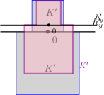
Figure 2: A nonconvex polygon $K^{\prime}$ and $y$ such that the total derivative of $f$ does not exist at $y$.

4 One more critical point

In this section, we prove Proposition 12. Given a manifold $M$ and a continuous function $f\colon M\to\mathbb{R}$ and $s\in\mathbb{R}$ we define the level set $L_{s}:=\{w\in M\colon f(w)=s\}$. In the proof of Proposition 12 we will need that the level sets are well-behaved in the neighborhoods of points $u$ for which the total derivative $Df(u)$ is nonzero.

Proposition 14.

Let $n\geq 1$, $f\colon\mathbb{R}^{n}\to\mathbb{R}$ be a $C^{1}$ function and $u\in\mathbb{R}^{n}$ be such that $Df(u)\neq 0$. Then there is a neighborhood $N(u)$ of $u$ such that for every $v,w\in N(u)$ if $f(v)=f(w)$, then $v$ and $w$ can be connected with a path within the level set $L_{f(v)}$. (It is allowed that this path leaves $N(u)$ provided that it stays in $L_{f(v)}$.)

Proof.

Without loss of generality assume that $\frac{\partial f}{\partial x_{n}}(u)>0$, otherwise we permute the coordinates and/or swap $x_{n}$ and $-x_{n}$. Consistently with the previous section, given $x\in\mathbb{R}^{n}$, we write $x=(\hat{x},x_{n})$ where $\hat{x}\in\mathbb{R}^{n-1}$ and $x_{n}\in\mathbb{R}$. Now we consider the $C^{1}$ function $F\colon\mathbb{R}^{n-1}\times\mathbb{R}\times\mathbb{R}\to\mathbb{R}$ defined as $F(\hat{x},t,x_{n}):=f(\hat{x},x_{n})-t$. Note that $\frac{\partial F}{\partial x_{n}}=\frac{\partial f}{\partial x_{n}}$. We also observe that $F(\hat{u},f(u),u_{n})=0$. Therefore, by the implicit function theorem, there is an open neighborhood $N^{\prime}$ of $(\hat{u},f(u))$ in $\mathbb{R}^{n-1}\times\mathbb{R}$ such that there is a $C^{1}$ function $g\colon N^{\prime}\to\mathbb{R}$ with $g(\hat{u},f(u))=u_{n}$ and that $F(\hat{v},t,g(\hat{v},t))=0$ for any $(\hat{v},t)\in N^{\prime}$. From the definition of $F$ this gives

$$f(\hat{v},g(\hat{v},t))=t.$$ (8)

By possibly restricting the neighborhood to a smaller set, we can assume that $N^{\prime}$ is the Cartesian product of a neighborhood $N^{\prime}(\hat{u})$ of $\hat{u}$ in $\mathbb{R}^{n-1}$ and $N^{\prime}(f(u))$ of $f(u)$ in $\mathbb{R}$, and that both $N^{\prime}(\hat{u})$ and $N^{\prime}(f(u))$ are open balls. Moreover, we can assume that $\frac{\partial F}{\partial x_{n}}(\hat{v},t,v_{n})>0$ for any $(\hat{v},t,v_{n})\in N^{\prime}\times N^{\prime\prime}(u_{n})$ where $N^{\prime\prime}(u_{n})$ is some neighborhood of $u_{n}$ in $\mathbb{R}$, again a ball. Now we possibly further restrict $N^{\prime}(\hat{u})$ and $N^{\prime}(f(u))$ so that $g(\hat{v},t)$ belongs to $N^{\prime\prime}(u_{n})$ for any $(\hat{v},t)\in N^{\prime}$.

The condition on the partial derivative of $F$ implies that for every $(\hat{v},t)\in N^{\prime}$ the equation $F(\hat{v},t,x_{n})=0$ has at most one solution $x_{n}\in N^{\prime\prime}(u_{n})$. Therefore it has a unique solution $x_{n}=g(\hat{v},t)$. In other words we get:

$$\hbox{If }f(\hat{v},x_{n})=t,\hbox{ then }x_{n}=g(\hat{v},t).$$ (9)

Now, we define $N(u):=\Psi^{-1}(N^{\prime})$ where $\Psi\colon\mathbb{R}^{n-1}\times\mathbb{R}\to\mathbb{R}^{n-1}\times\mathbb{R}$ is defined as $\Psi(v)=(\hat{v},f(v))$ for any $v\in\mathbb{R}^{n-1}\times\mathbb{R}$. In particular $(\hat{v},f(v))$ belongs to $N^{\prime}$ for any $v\in N(u)$.

Let $t:=f(v)=f(w)$. From (9) we get $v_{n}=g(\hat{v},t)$ and $w_{n}=g(\hat{w},t)$. Let us consider an arbitrary path $P\colon[0,1]\to N^{\prime}(\hat{u})$ connecting $\hat{v}$ and $\hat{w}$. Let us ‘lift’ $P$ to a path $P_{t}\colon[0,1]\to\mathbb{R}^{n-1}\times\mathbb{R}$ given by $P_{t}(s):=(P(s),g(P(s),t))$. This is a path connecting $v$ and $w$. We will be done once we show $P_{t}([0,1])\subseteq L_{t}$. This means that we are supposed to show that $f(P(s),g(P(s),t))=t$ for every $s\in[0,1]$ which follows from (8). ∎

Total derivatives and gradients.

Let $f\colon\mathbb{R}^{n}\to\mathbb{R}$ be a $C^{1}$ function. Then for any $u\in\mathbb{R}^{n}$, the total derivative $Df(u)$ is represented by a row vector $\left(\frac{\partial}{\partial x_{1}}f(u),\dots,\frac{\partial}{\partial x_{n}}f(u)\right)$ (if $Df(u)$ exists). By $\|Df(u)\|$ we mean the Euclidean norm of this vector. The gradient $\nabla f(u)$ is the same vector transposed

$$\nabla f(u):=\left(\frac{\partial}{\partial x_{1}}f(u),\dots,\frac{\partial}{\partial x_{n}}f(u)\right)^{T}.$$

Then $\|\nabla f(u)\|=\|Df(u)\|$, and in addition $Df(u)(\nabla f(u))=\|Df(u)\|^{2}$.

Let $x\in\mathbb{R}^{n}$ and $\rho>0$, by $B(x,\rho)\subseteq\mathbb{R}^{n}$ we denote the compact ball of radius $\rho$ centered in $x$ with respect to the standard Euclidean metric.

Lemma 15.

Let $f\colon\mathbb{R}^{n}\to\mathbb{R}$ be a $C^{1}$ function, let $x\in\mathbb{R}^{n}$ and let $\zeta,\rho>0$. Assume that $\|Df(u)\|\geq\zeta$ for every $u\in B(x,\rho)$. Then there is $v\in B(x,\rho)$ such that $f(v)\geq f(x)+\frac{\zeta\rho}{2}$.

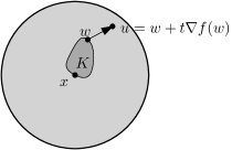
Figure 3: The set $K$ inside $B(x,\rho)$. For contradiction $M<f(x)+\frac{\rho\zeta}{2}$ which implies that $K$ does not touch the boundary of the ball. Then $t>0$ can be chosen so that $u=w+t\nabla f(w)$ still belongs to $B(x,\rho)$.

Proof.

Let

$$K:=\{y\in B(x,\rho)\colon f(y)\geq f(x)+\frac{\zeta}{2}\|y-x\|\}.$$

This is a closed therefore compact set, it is also nonempty because $x\in K$. Let $M:=\max\{f(y)\colon y\in K\}$, for contradiction $M<f(x)+\frac{\zeta\rho}{2}$. Let $w\in K$ be such that $f(w)=M$. Note that for every $v\in\partial B(x,\rho)\cap K$ we get $f(v)\geq f(x)+\frac{\zeta\rho}{2}$ because $\|v-x\|=\rho$ in this case. Thus, in particular, $w\not\in\partial B(x,\rho)$. See Figure 3.

Consider the derivative at $w$ in the direction of the gradient $\nabla f(w)$. From properties of the total derivative, we get

$$\lim_{t\to 0}\frac{|f(w+t\nabla f(w))-f(w)-Df(w)(t\nabla f(w))|}{t\|\nabla f(w)\|}=0.$$

Therefore, for small enough $t>0$ we get

$$|f(w+t\nabla f(w))-f(w)-t\|Df(w)\|^{2}|\leq\frac{\zeta}{2}t\|Df(w)\|.$$

Consequently,

$$f(w)+t\|Df(w)\|^{2}-f(w+t\nabla f(w))\leq\frac{\zeta}{2}t\|Df(w)\|.$$

Let $u=w+t\nabla f(w)$. If $t$ is small enough then $u\in B(x,\rho)$. Using $\|Df(w)\|\geq\zeta$ this gives

$$f(u)\geq f(w)+t\|Df(w)\|^{2}-\frac{\zeta}{2}t\|Df(w)\|\geq f(w)+\frac{\zeta}{2}t\|Df(w)\|=f(w)+\frac{\zeta}{2}t\|\nabla f(w)\|.$$ (10)

Because $w\in K$ and $t\|\nabla f(w)\|=\|u-w\|$, we further get

$$f(u)\geq f(x)+\frac{\zeta}{2}(\|w-x\|+\|u-w\|)\geq f(x)+\frac{\zeta}{2}(\|u-x\|).$$ (11)

Equation (11) gives that $u\in K$ while (10) gives $f(u)>M$. This is a contradiction with the choice of $M$. ∎

Proof of Proposition 12.

First, we can assume that all local extrema $m_{1},\dots,m_{k}$ are strict. Indeed, if some of them is not strict, say $m_{1}$, then we can find $u\neq m_{1},\dots,m_{k}$ with $Df(u)=0$ in a neighborhood of $m_{1}$.

Next, because $k\geq 3$, there are at least two local maxima or two local minima among $m_{1},\dots,m_{k}$. Without loss of generality, $m_{1}$ and $m_{2}$ are local maxima.

Now, let us consider a path $\gamma\colon[0,1]\to S^{n}$ such that $\gamma(0)=m_{1}$ and $\gamma(1)=m_{2}$. Let $\min_{f}(\gamma):=\min\{f(\gamma(t))\colon t\in[0,1]\}$ (the minimum exists by compactness) and let $s:=\sup(\min_{f}(\gamma))$ where the supremum is taken over all $\gamma$ as above.

Before we proceed with the formal proof, let us sketch the main idea of the proof; see also Figure 4. For contradiction assume that $Df(u)\neq 0$ for every $u\in S^{n}\setminus\{m_{1},\dots,m_{k}\}$. Consider $\gamma$ such that $\min_{f}(\gamma)$ is very close to $s$. We will be able to argue that we can assume that such $\gamma$ is not close to any of the other extremes $m_{3},\dots,m_{k}$. This guarantees that $\|Df(\gamma(t))\|$ is bounded from $0$ for every $t\in[0,1]$ except the cases when $\gamma(t)$ is close to $m_{1}$ or $m_{2}$. Using Lemma 15, we will be able to modify $\gamma$ to $\gamma^{\prime}$ with $\min_{f}(\gamma^{\prime})>s$ obtaining a contradiction with the definition of $s$.

Figure 4: If we are in mountains and we want to hike from one peak to another without losing too much altitude, then the best way is to pass through a saddle point (see the upper path in blue). If we do not pass very close to a saddle point, then the positive gradient allows us to improve the path (see the lower path in red).

In further consideration, we consider the standard metric on $S^{n}$ obtained by the standard embedding of $S^{n}$ into $\mathbb{R}^{n+1}$ and restricting the Euclidean metric on $\mathbb{R}^{n+1}$ to a metric on $S^{n}$. For every $i\in[k]$, we pick two closed metric balls $B_{i}$ and $B^{\prime}_{i}$ centered in $m_{i}$. Namely, $B_{i}$ is chosen so that $m_{i}$ is a global extreme on $B_{i}$. We also assume that the balls $B_{i}$ are pairwise disjoint. Next, we distinguish whether $m_{i}$ is a local maximum or minimum. If $m_{i}$ is a local maximum, let us define $a_{i}:=\max\{f(x)\colon x\in\partial B_{i}\}$. Note that $f(m_{i})>a_{i}$ as $m_{i}$ is a global maximum on $B_{i}$. Then we pick a closed ball $B^{\prime}_{i}$ centered in $m_{i}$ inside $B_{i}$ so that $f(x)>a_{i}$ for every $x\in B^{\prime}_{i}$. If $m_{i}$ is a local minimum, we proceed analogously. We set $a_{i}:=\min\{f(x)\colon x\in\partial B_{i}\}$ and we pick $B^{\prime}_{i}$ so that $f(x)<a_{i}$ for every $x\in B^{\prime}_{i}$. For later use, we also define $a^{\prime}_{i}:=\min\{f(x)\colon x\in B^{\prime}_{i}\}$ for $i\in\{1,2\}$. Note that $a^{\prime}_{i}>a_{i}$.

Given a path $\gamma$ connecting $m_{1}$ and $m_{2}$, we say that $\gamma$ is avoiding if it does not pass through the interior of any of the balls $B^{\prime}_{3},\dots,B^{\prime}_{k}$.

Claim 15.1.

Let $\gamma$ be a path connecting $m_{1}$ and $m_{2}$. Then there is an avoiding path $\bar{\gamma}$ connecting $m_{1}$ and $m_{2}$ such that $\min_{f}(\bar{\gamma})\geq\min_{f}(\gamma)$.

Proof.

Assume that $\gamma$ enters a ball $B^{\prime}_{i}$ for $i\in\{3,\dots,k\}$. Let us distinguish whether $m_{i}$ is a local maximum or minimum.

First assume that $m_{i}$ is a local maximum. Then $\min_{f}(\gamma)\leq a_{i}$ because $\gamma$ has to pass through $\partial B_{i}$. By a homotopy, fixed outside the interior of $B^{\prime}_{i}$ we can assume that $\gamma$ avoids $m_{i}$ (here we use $n\geq 2$); see, e.g., the proof of Proposition 1.14 in [Hat02] how to perform this step. In addition, by further homotopy fixed outside the interior of $B^{\prime}_{i}$ we can modify $\gamma$ so that it avoids the interior of $B^{\prime}_{i}$ (the second homotopy pushes $\gamma$ in direction away from $m_{i}$). This does not affect $\min_{f}(\gamma)$ because $f(x)>a_{i}$ for every $x\in B^{\prime}_{i}$.

Next let us assume that $m_{i}$ is a local minimum. Then $\min_{f}(\gamma)<a_{i}$ because $\gamma$ has to pass through $\partial B^{\prime}_{i}$ (this is not a symmetric argument when compared with the previous case). Modify $\gamma$ by analogous homotopies as above; however, this time with respect to $B_{i}$ (so that $\gamma$ completely avoids the interior of $B_{i}$). Because $\min_{f}(\gamma)<a_{i}$ and $f(x)\geq a_{i}$ for $x\in\partial B_{i}$, the minimum of $\gamma$ cannot decrease by these modifications. By performing these modifications for all $B^{\prime}_{i}$ when necessary, we get the required $\bar{\gamma}$. ∎

Now, let us consider a diffeomorphism $\psi\colon S^{n}\setminus\{m_{k}\}\to\mathbb{R}^{n}$ given by the stereographic projection (in particular, it maps closed balls avoiding $m_{k}$ to closed balls). Let $g\colon\mathbb{R}^{n}\to\mathbb{R}$ be defined as $g:=f\circ\psi^{-1}$. Let $n_{i}:=\psi(m_{i})$ for $i\in[k-1]$. Once we find $v\in\mathbb{R}^{n}$, $v\neq n_{1},\dots,n_{k-1}$ such that $Dg(v)=0$, then $u:=\psi^{-1}(v)$ is the required point with $Df(u)=0$. Note that $n_{1},n_{2}$ are still local maxima of $g$ and $n_{3},\dots,n_{k-1}$ are local maxima or minima. We also set $D_{i}:=\psi(B_{i})$ and $D^{\prime}_{i}:=\psi(B^{\prime}_{i})$ for $i\in[k-1]$ and $C_{k}:=\psi(B_{k}\setminus\{m_{k}\})$, $C^{\prime}_{k}:=\psi(B^{\prime}_{k}\setminus\{m_{k}\})$. The sets $D_{i}$ and $D^{\prime}_{i}$ are closed (metric) balls centered in $n_{i}$ whereas $C_{k}$ and $C^{\prime}_{k}$ are complements of open (metric) balls in $\mathbb{R}^{n}$. Let $K$ be the compact set obtained from $\mathbb{R}^{n}$ by removing the interiors of $D^{\prime}_{1},\dots,D^{\prime}_{k-1},C^{\prime}_{k}$. Let us fix small enough $\eta>0$ such that the closed $\eta$-neighborhoood $K_{\eta}$ of $K$ avoids $n_{1},\dots,n_{k-1}$. We will also use the notation $K_{\eta/3}$ for the closed $\frac{\eta}{3}$-neighborhood of $K$. See Figure 5.

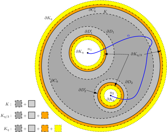
Figure 5: The sets $K$, $K_{\eta/3}$ and $K_{\eta}$ and some path $\alpha$ connecting $n_{1}$ and $n_{2}$ of the form $\alpha=\psi\circ\gamma$ where $\gamma$ is avoiding. In the picture, $k=3$.

Assume, for contradiction, that $K_{\eta}$ does not contain $v$ with $Dg(v)=0$. Because $K_{\eta}$ is compact and $g$ is $C^{1}$, there is $\zeta>0$ such that $\|Dg(w)\|\geq\zeta$ for every $w\in K_{\eta}$.

For every $w\in K_{\eta/3}$ let $N(w)$ be the neighborhood given by Proposition 14 (the neighborhood is considered in the whole $\mathbb{R}^{n}$ not only in $K_{\eta/3}$). By possibly restricting $N(w)$ to smaller sets, we can assume that each $N(w)$ is open and fits into a ball of radius $\frac{2}{3}\eta$. (In particular, if $w\in K_{\eta/3}$, then $N(w)\subseteq K_{\eta}$.)

Claim 15.2.

There is $\varepsilon>0$ such that for every $x\in K_{\eta/3}$ the metric ball $B(x,\varepsilon)\subseteq\mathbb{R}^{n}$ centered in $x$ of radius $\varepsilon$ fits into $N(w)$ for some $w\in K_{\eta/3}$.

Proof.

This is just a modification of the Lebesgue number lemma. Let us consider the open cover $\mathcal{O}$ of $K_{\eta}$ consisting of all sets $N(w)$ together with the relative interiors of the sets $B^{\prime}_{1}\cap(K_{\eta}\setminus K_{\eta/3}),\dots,B^{\prime}_{k-1}\cap(K_{\eta}\setminus K_{\eta/3}),C^{\prime}_{k}\cap(K_{\eta}\setminus K_{\eta/3})$ (all sets are relatively open in $K_{\eta}$). Note that the newly added sets are disjoint from $K_{\eta/3}$. Let $\varepsilon>0$ be the standard Lebesgue number with respect to the cover $\mathcal{O}$, that is, for every $x\in K_{\eta}$, the ball $B(x,\varepsilon)$ fits into one of the sets of $\mathcal{O}$; see [Mun13, Lemma 27.5]. Then the required claim holds with this $\varepsilon$ because if $x\in K_{\eta/3}$, then $x$ does not belong to any of the newly added sets of $\mathcal{O}$. ∎

Let $\varepsilon$ be the value obtained from Claim 15.2. Because some ball $B(x,\varepsilon)$ fits into some $N(w)$ which fits into a ball of radius $\frac{2}{3}\eta$, we get $\varepsilon\leq\frac{2}{3}\eta$.

Let us consider a path $\gamma$ in $S^{n}$ such that

1. $s-\min_{f}(\gamma)<a^{\prime}_{1}-a_{1}$;

2. $s-\min_{f}(\gamma)<a^{\prime}_{2}-a_{2}$; and

3. $s-\min_{f}(\gamma)<\frac{\zeta\varepsilon}{4}$.

By Claim 15.1, we can assume that $\gamma$ is avoiding. We will start modifying $\gamma$ to $\gamma^{\prime}$ with $\min_{f}(\gamma^{\prime})>s$, which will be the required contradiction. Let $\alpha:=\psi\circ\gamma$; see the diagram at Figure 6. Then $\alpha$ connects $n_{1}$ and $n_{2}$, and $\alpha$ avoids the interiors of $D^{\prime}_{3},\dots,D^{\prime}_{k-1}$ and $C^{\prime}_{k}$; see Figure 5.

Figure 6: The maps $\alpha$, $\gamma$, $\psi$, $f$ and $g$. The two triangles are commutative.

Because, $\alpha$ is a continuous function on the compact interval $[0,1]$, we get, by the Heine-Cantor theorem, that $\alpha$ is uniformly continuous. In particular, there is $\delta>0$ such that if $t_{1},t_{2}\in[0,1]$ with $|t_{1}-t_{2}|\leq\delta$, then $\|\alpha(t_{1})-\alpha(t_{2})\|\leq\frac{\varepsilon}{3}$. Let us consider a positive integer $\ell>\frac{1}{\delta}$. We will be modifying $\alpha$ in two steps. First, we get $\alpha^{\prime\prime}$ such that $\alpha^{\prime\prime}(t)>s$ if $t=\frac{j}{\ell}$ for some $j\in\{0,\dots,\ell\}$. Then we modify $\alpha^{\prime\prime}$ individually on the intervals $(\frac{j}{\ell},\frac{j+1}{\ell})$ for $j\in\{0,\dots,\ell-1\}$ obtaining $\alpha^{\prime}$ with $\min_{g}(\alpha^{\prime})>s$. (Given a path $\beta\colon[0,1]\to\mathbb{R}^{n}$ connecting $n_{1}$ and $n_{2}$, we define $\min_{g}(\beta):=\min\{g(\beta(t))\colon t\in[0,1]\}=\min_{f}(\psi^{-1}\circ\beta)$.) The required $\gamma^{\prime}$ will be obtained as $\psi^{-1}\circ\alpha^{\prime}$.

For the first step, let us first say that an interval $I_{j}=[\frac{j}{\ell},\frac{j+1}{\ell}]$ where $j\in\{0,\dots,\ell-1\}$ requires a modification if $g(\alpha(t))\leq s$ for some $t\in I_{j}$. This in particular means that $\alpha(t)\in K$ for this $t$: Indeed, this follows from (s1) and (s2). We already know that $\alpha$ avoids the interiors of $D^{\prime}_{3},\dots,D^{\prime}_{k-1}$ and $C^{\prime}_{k}$. It remains to check that $\alpha(t)$ does not belong to the interiors of $D^{\prime}_{1}$ and $D^{\prime}_{2}$ as well. Because $\alpha$ has to meet $\partial D_{1}$ and $\partial D_{2}$, we get that $\min_{f}(\gamma)=\min_{g}(\alpha)\leq a_{1},a_{2}$ from the definition of $a_{1}$ and $a_{2}$. By (s1) and (s2), we get $s<a^{\prime}_{1},a^{\prime}_{2}$. Therefore, from the definition of $a^{\prime}_{1}$ and $a^{\prime}_{2}$, we get that $\alpha(t)$ cannot belong neither to $D^{\prime}_{1}$ nor to $D^{\prime}_{2}$ as required.

By the uniform continuity, the fact that $g(\alpha(t))\leq s$ for some $t\in I_{j}$ implies that $\alpha(I_{j})$ belongs to the closed $\frac{\varepsilon}{3}$-neighborhood of $K$. In particular, $\alpha(I_{j})$ belongs to $K_{\eta/3}$ as $\varepsilon\leq\frac{2}{3}\eta<\eta$.

Now, for each $I_{j}$ which requires a modification, consider the open $\varepsilon$-ball $U_{j}\subseteq\mathbb{R}^{n}$ centered in $\alpha(\frac{2j+1}{2\ell})$. (Note that, $\frac{2j+1}{2\ell}$ is the midpoint of $I_{j}$.) From the previous considerations, the centre of each $U_{j}$ belongs to $K_{\eta/3}$ and the whole $U_{j}$ is a subset of $K_{\eta}$.

Now we perform the first step. Consider $t=\frac{j}{\ell}$ for some $j\in\{0,\dots,\ell\}$. If $g(\alpha(t))>s$, then we do nothing. Note that this includes the cases $j=0$ or $j=\ell$. If $g(\alpha(t))\leq s$, then both intervals $I_{j-1}$ and $I_{j}$ require a modification. By the uniform continuity, the open ball $V_{j}\subseteq\mathbb{R}^{n}$ centered in $\alpha(t)$ of radius $\frac{2\varepsilon}{3}$ is a subset of both $U_{j-1}$ and $U_{j}$; see Figure 7. We observe that $V_{j}$ is a subset of $K_{\eta}$ as $V_{j}\subseteq U_{j}$. In particular, by the definition of $\zeta$, we get that $\|Dg(w)\|\geq\zeta$ for every $w\in V_{j}$. By Lemma 15, used on a closed ball of a slightly smaller radius $\frac{\varepsilon}{2}$, there is a point $v$ in $V_{j}$ such that

$$g(v)\geq g(\alpha(t))+\frac{\zeta\varepsilon}{4}\geq{\textstyle\min_{g}(\alpha)}+\frac{\zeta\varepsilon}{4}={\textstyle\min_{f}(\gamma)}+\frac{\zeta\varepsilon}{4}.$$

Using (s3), we get $g(v)>s$. Now, by a homotopy, we modify $\alpha$ to $\alpha^{\prime\prime}$ so that it stays fixed outside the interval $(t-\frac{1}{4\ell},t+\frac{1}{4\ell})$, the modification of $\alpha$ occurs only in $V_{j}$ and $\alpha^{\prime\prime}(t)=v$; see Figure 8. We perform these modifications simultaneously for every $t=\frac{j}{\ell}$ with $g(\alpha(t))\leq s$. This is possible as the intervals $[t-\frac{1}{4\ell},t+\frac{1}{4\ell}]$ are pairwise disjoint. This way, we obtain the required $\alpha^{\prime\prime}$.

Figure 7: The sets $U_{j-1}$, $U_{j}$ and $V_{j}$ in the case that $g(\alpha(\frac{j}{\ell}))\leq s$.

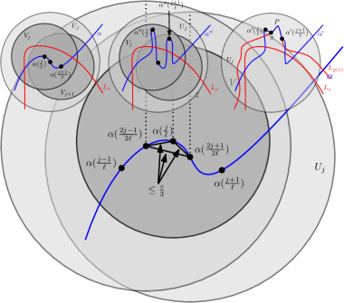
Figure 8: The first and the second step of modifications of $\alpha$ on an interval $I_{j}$ requiring a modification (the modification is shown only on this interval).

Finally, we perform the second step of the modification. Let $I_{j}=[\frac{j}{\ell},\frac{j+1}{\ell}]$ be an interval requiring a modification. We already know that $g(\alpha^{\prime\prime}(\frac{j}{\ell}))>s$ and $g(\alpha^{\prime\prime}(\frac{j+1}{\ell}))>s$. In addition, we know that both $\alpha^{\prime\prime}(\frac{j}{\ell})$ and $\alpha^{\prime\prime}(\frac{j+1}{\ell})$ belong to $U_{j}$ as they belong to $V_{j}$ or $V_{j+1}$. We set $\alpha^{\prime}(\frac{j}{\ell}):=\alpha^{\prime\prime}(\frac{j}{\ell})$ and $\alpha^{\prime}(\frac{j+1}{\ell}):=\alpha^{\prime\prime}(\frac{j+1}{\ell})$. Next, we aim to define $\alpha^{\prime}$ on $(\frac{j}{\ell},\frac{j+1}{\ell})$, which is the interior of $I_{j}$, so that $\min(g(\alpha^{\prime}(I_{j})))>s$. By Claim 15.2, $U_{j}$ fits into some $N(w)$ for some $w\in K_{\eta/3}$. (Here we use that the center of $U_{j}$ belongs to $K_{\eta/3}$.) Now, Proposition 14 implies that $\alpha^{\prime}(\frac{j}{\ell})$ and $\alpha^{\prime}(\frac{j+1}{\ell})$ may be connected by a path $P\colon[0,1]\to\mathbb{R}^{n}$ such that $g(P(t))>s$ for every $t\in[0,1]$: Indeed, let us assume that, without loss of generality, $g(\alpha^{\prime}(\frac{j}{\ell}))\geq g(\alpha^{\prime}(\frac{j+1}{\ell}))>s$. First, draw $P$ as a straight line from $\alpha^{\prime}(\frac{j}{\ell})$ towards $\alpha^{\prime}(\frac{j+1}{\ell})$ until we reach a (first) point $x\in U_{j}\subseteq N(w)$ with $g(x)=g(\alpha^{\prime}(\frac{j+1}{\ell}))$; of course, it may happen that $x=\alpha^{\prime}(\frac{j+1}{\ell})$. Then by Proposition 14, $x$ and $\alpha^{\prime}(\frac{j}{\ell})$ can be connected within the level set $L_{g(x)}$; see Figure 8. (This may mean that $P$ leaves $N(w)$, or even $K_{\eta}$, but this is not problem for the argument.) Altogether, we set $\alpha^{\prime}$ on $I_{j}$ so that it follows the path $P$, and this we do independently on each interval requiring a modification. Other intervals remain unmodified.

From the construction, we get $\min_{g}(\alpha^{\prime})>s$; therefore the path $\gamma^{\prime}:=\psi^{-1}\circ\alpha^{\prime}$ satisfies $\min_{f}(\gamma^{\prime})=\min_{g}(\alpha^{\prime})>s$ which contradicts the definition of $s$. ∎

5 Depth-like functions with few critical points

Bipyramid over a triangle.

In $\mathbb{R}^{3}$, we have a candidate example of a convex body, namely the regular bipyramid $B$ over an equilateral triangle $T$, such that there are exactly four barycentric hyperplanes (with respect to the barycenter of $B$, which coincides with the point of maximal depth in this case). On the one hand, this is not surprising, because this is $n+1$ hyperplanes, where $n=3$ is the dimension of the ambient space. On the other hand, if this is true, then it answers negatively, in dimension $3$, a question from [CFG94, A8], whether $2^{n}-1$ barycentric hyperplanes always exist.

More concretely, we conjecture that the only barycentric hyperplanes are the following: three planes perpendicular to $T$ which meet $T$ in lines realizing the depth of $T$ (these would be the hyperplanes realizing the depth), and the plane of $T$ (this is the one extra plane). Unfortunately, in this case, it is not so easy to analyze the depth function as in the case of $T\times I$.

A function with four critical points and many properties of the depth.

Let us recall that the depth function $\delta\colon S^{n-1}\to[0,1]$ on a convex body satisfies the following properties:

1. $\delta(v)=1-\delta(-v)$;

2. $0\in\operatorname{conv}U$ where $U\subseteq S^{n-1}$ is the set of the points where $\delta$ attains the minimum (by Proposition 8);

3. $|U|\geq 3$, (by Corollary 9);

4. $\delta$ is $C^{1}$ (by Proposition 11);

5. if $U$ is finite, then $\delta$ has at least one more pair of opposite critical points (by Proposition 12 and by (i)).

We will show that our argument in the proof of Theorem 10 is tight in the sense that for $n\geq 3$ there exists a function $\delta^{\prime}\colon S^{n-1}\to[0,1]$ satisfying (i)–(v) with equalities in (iii) and (v).

In order to define $\delta^{\prime}$, it will be much more convenient to reparametrize $\delta^{\prime}$. Thus, we will exhibit $\delta^{\prime\prime}\colon S^{n-1}\to[-1,1]$ which satisfies (ii)–(v) with equalities in (iii) and (v) but $\delta^{\prime\prime}(v)=-\delta^{\prime\prime}(-v)$ instead of (i). Then the required $\delta^{\prime}$ is obtained as $\frac{1}{2}\delta^{\prime\prime}+\frac{1}{2}$.

This time we decompose $\mathbb{R}^{n}$ as $\mathbb{R}^{n-2}\times\mathbb{R}^{2}$ and for a point $x\in\mathbb{R}^{n}$ we write $x=(y;z)$ where $y=(y_{1},\dots,y_{n-2})\in\mathbb{R}^{n-2}$ and $z=(z_{1},z_{2})\in\mathbb{R}^{2}$. The idea is to define $\delta^{\prime\prime}$ separately on the sphere $S^{n-3}\times\{0\}$ so that there is only one pair of opposite critical points here (this will be the extra pair from (v)), separately on the sphere $\{0\}\times S^{1}$ so that there are three pairs of critical points (these will be three global minima and three global maxima from (iii)), and then merge the two constructions so that the resulting function is smooth and no new critical points arise. Unfortunately, the details are somewhat tedious.

We actually define $\delta^{\prime\prime}$ on $\mathbb{R}^{n}\setminus\{0\}$ considering $S^{n-1}$ as a subset of $\mathbb{R}^{n}\setminus\{0\}$. Now, we set

$$\delta^{\prime\prime}(y,z)=\frac{1}{10}(2\|y\|-\|y\|^{3})y_{1}+\frac{1}{2}\|z\|(z_{1}^{3}-z_{1}z_{2}^{2}-2z_{1}z_{2}^{2}).$$ (12)

We remark that the expression $(z_{1}^{3}-z_{1}z_{2}^{2}-2z_{1}z_{2}^{2})$ is nothing else then the real part $\Re(z^{3})$, where $z=(z_{1},z_{2})$ is identified with the complex number $z_{1}+iz_{2}$. From (12) we easily see that $\delta^{\prime\prime}$ is smooth on $\mathbb{R}^{n}\setminus\{0\}$, therefore its restriction to $S^{n-1}$ is smooth as well as the inclusion $S^{n-1}\subseteq\mathbb{R}^{n}\setminus\{0\}$ is a smooth embedding. We also easily check that $\delta^{\prime\prime}(y,z)=-\delta^{\prime\prime}(-y,-z)$.

From now on, let us assume that $(y,z)\in S^{n-1}$, that is $\|y\|^{2}+\|z\|^{2}=1$. If $y\neq 0$, we get

$$(2\|y\|-\|y\|^{3})y_{1}=(1-(1-\|y\|^{2})^{2})\frac{y_{1}}{\|y\|}=(1-\|z\|^{4})\frac{y_{1}}{\|y\|},$$ (13)

and if $z\neq 0$, we get (in complex numbers)

$$\|z\|(z_{1}^{3}-z_{1}z_{2}^{2}-2z_{1}z_{2}^{2})=\|z\|^{4}\frac{\Re(z^{3})}{\|z\|^{3}}=\|z\|^{4}\Re((z/\|z\|)^{3}).$$ (14)

Altogether (12), (13) and (14) give

$$\delta^{\prime\prime}(y,z)=\begin{cases}(1-\|z\|^{4})\frac{1}{10}\frac{y_{1}}{\|y\|}+\|z\|^{4}\frac{1}{2}\Re((z/\|z\|)^{3})\hbox{ if }y,z\neq 0,\\ \frac{1}{2}\Re(z^{3})\hbox{ if }y=0,\\ \frac{1}{10}y_{1}\hbox{ if }z=0.\\ \end{cases}$$ (15)

In particular, (15) implies that for $y,z\neq 0$, $\delta^{\prime\prime}(y,z)$ is a convex combination of $\frac{1}{10}\frac{y_{1}}{\|y\|}$ and $\frac{1}{2}\Re((z/\|z\|)^{3})$, which attain values in $[-1/10,1/10]$ and $[-1/2,1/2]$ respectively. Therefore $\delta^{\prime\prime}(S^{n-1})\subseteq[-1/2,1/2]$.

Now we check that $\delta^{\prime\prime}$ attains exactly three global minima on $S^{n-1}$. We observe that $\delta^{\prime\prime}(0,e^{i(2k+1)/3)\pi})=-1/2$ for $k=0,1,2$ by (15). Therefore $\delta^{\prime\prime}$ attains the minimum at these three points. On the other hand, we realize that these are the only three points where $\delta^{\prime\prime}(y,z)=-1/2$. Indeed, if $y=0$, then $\delta^{\prime\prime}(y,z)=-1/2$ only if $\Re(z^{3})=-1$, which occurs only if $z=e^{i(2k+1)\pi/3}$ for $k=0,1,2$. If $z=0$, then $\delta^{\prime\prime}(y,z)\geq-1/10$ by (15). Finally, if $y,z\neq 0$, then the convex combination from (15) has the strictly positive coefficient $(1-\|z\|^{4})$ at $\frac{1}{10}\frac{y_{1}}{\|y\|}$, which implies $\delta^{\prime\prime}(y,z)>\frac{1}{2}\Re((z/\|z\|)^{3})\geq-1/2$. This characterization of global minima also gives property (ii).

It remains to check that there is exactly one extra pair of opposite critical points of $\delta^{\prime\prime}$. This could be done via Lagrange multipliers but the computations seem to be slightly tedious, thus we provide a different argument. In advance, we announce that these extra critical points will be $(e_{1},0)$ and $(-e_{1},0)$, where $e_{1}\in S^{n-3}\subseteq\mathbb{R}^{n-2}$ is the first coordinate vector $e_{1}=(1,0,\dots,0)$. We will rule out all other options, thus these points have to be indeed critical by Proposition 12.

Let $(y,z)\in S^{n-1}$ be a critical point. If $y=0$, then $\delta^{\prime\prime}(0,z)=\frac{1}{2}\Re(z^{3})$ by (15) when restricted to $\{0\}\times S^{1}\subseteq S^{n-1}$ (where $0\in\mathbb{R}^{n-2}$ in this case). Therefore $(0,z)$ has to be critical point of the restriction as well. It is easy to analyse that the only critical points of $\frac{1}{2}\Re(z^{3})$ are of the form $z=e^{ik\pi/3}$ where $k\in\{0,\dots,5\}$, which are the minima and the maxima opposite to the minima. If $z=0$, then $\delta^{\prime\prime}(y,0)=\frac{1}{10}y_{1}$ when restricted to $S^{n-3}\times\{0\}\subseteq S^{n-1}$ (where $0\in\mathbb{R}^{2}$ in this case). Again, it is easy to analyze that $e_{1}$ and $-e_{1}$ are the only critical points. (Here they are the maximum and minimum in the restriction respectively, but they are not even local extremes on whole $S^{n-1}$.) Finally, we consider the case $y,z\neq 0$. First, we fix $y$ and let $z$ vary subject to $\|y\|^{2}+\|z\|^{2}=1$, which implies that $\|z\|$ is fixed as well. Then $\delta^{\prime\prime}(y,z)=a_{y}+b_{y}\Re((z/\|z\|)^{3})$ by (15) where $a_{y}$ and $b_{y}$ are constants depending on $y$. This implies that if $(y,z)$ is critical, then $z/\|z\|=e^{ik\pi/3}$ where $k\in\{0,\dots,5\}$. Next, we fix $z$ and let $y$ vary. By a similar idea as above, we deduce that if $(y,z)$ is critical, then $y=(\pm y_{1},0,\dots,0)$. Finally, let us fix both $y$ and $z$ and consider the $2$-plane $\rho(y,z)$ given by all vectors $(t_{y}y,t_{z}z)$ for $t_{y},t_{z}\in\mathbb{R}$. This $2$-plane meets $S^{n-1}$ in a circle. For $(t_{y}y,t_{z}z)$ in $\rho(y,z)\cap S^{n-1}$ the equation (15) gives

$$\delta^{\prime\prime}(t_{y},t_{z}) =(1-t_{z}^{4}\|z\|^{4})\frac{1}{10}\frac{y_{1}}{\|y\|}+t_{z}^{4}\|z\|\frac{1}{2}\Re((z/\|z\|)^{3})$$

$$=\frac{1}{10}\frac{y_{1}}{\|y\|}+t_{z}^{4}\|z\|^{4}\left(\frac{1}{2}\Re((z/\|z\|)^{3})-\frac{1}{10}\frac{y_{1}}{\|y\|}\right).$$

Therefore $(t_{y}y,t_{z}z)$, for $t_{y},t_{z}\neq 0$, may be the critical point of $\delta^{\prime\prime}$ only if

$$\frac{1}{2}\Re((z/\|z\|)^{3})=\frac{1}{10}\frac{y_{1}}{\|y\|}$$ (16)

which is independent of the values $t_{y}$ and $t_{z}$. If we recall the previous two conditions on the critical point $(y,z)$, we get $\Re((z/\|z\|)^{3})=\pm 1$ and $\frac{y_{1}}{\|y\|}=\pm 1$, therefore (16) may not hold simultaneously. This finishes the analysis of the critical points of $\delta^{\prime\prime}$.

References

- [BCI+08] D. Bremner, D. Chen, J. Iacono, S. Langerman, and P. Morin. Output-sensitive algorithms for Tukey depth and related problems. Stat. Comput., 18(3):259–266, 2008.
- [BK16] P. Blagojević and R. Karasev. Local multiplicity of continuous maps between manifolds, 2016. Preprint; https://arxiv.org/abs/1603.06723.
- [Bla17] W. Blaschke. Über affine Geometrie IX: Verschiedene Bemerkungen und Aufgaben. Ber. Verh. Sächs. Akad. Wiss. Leipzig. Math.-Nat. Kl., 69:412–420, 1917.
- [CFG94] H. T. Croft, K. J. Falconer, and R. K. Guy. Unsolved problems in geometry. Problem Books in Mathematics. Springer-Verlag, New York, 1994. Corrected reprint of the 1991 original, Unsolved Problems in Intuitive Mathematics, II.
- [Cha04] T. M. Chan. An optimal randomized algorithm for maximum Tukey depth. In Proceedings of the Fifteenth Annual ACM-SIAM Symposium on Discrete Algorithms, pages 430–436. ACM, New York, 2004.
- [CMW13] D. Chen, P. Morin, and U. Wagner. Absolute approximation of Tukey depth: theory and experiments. Comput. Geom., 46(5):566–573, 2013.
- [DG92] D. L. Donoho and M. Gasko. Breakdown properties of location estimates based on halfspace depth and projected outlyingness. Ann. Statist., 20(4):1803–1827, 1992.
- [DM16] R. Dyckerhoff and P. Mozharovskyi. Exact computation of the halfspace depth. Comput. Statist. Data Anal., 98:19–30, 2016.
- [Don82] D. L. Donoho. Breakdown properties of multivariate location estimators., 1982. Unpublished qualifying paper, Harvard University.
- [Dup22] C. Dupin. Applications de géométrie et de méchanique, a la marine, aux ponts et chaussées, etc., pour faire suite aux Développements de géométrie, par Charles Dupin.. Bachelier, successeur de Mme. Ve. Courcier, libraire, 1822.
- [Grü61] B. Grünbaum. On some properties of convex sets. Colloq. Math., 8:39–42, 1961.
- [Grü63] B. Grünbaum. Measures of symmetry for convex sets. In Proc. Sympos. Pure Math., Vol. VII, pages 233–270. Amer. Math. Soc., Providence, R.I., 1963.
- [Hat02] A. Hatcher. Algebraic topology. Cambridge University Press, Cambridge, 2002.
- [HR08] A. Hassairi and O. Regaieg. On the Tukey depth of a continuous probability distribution. Statist. Probab. Lett., 78(15):2308–2313, 2008.
- [Kar11] R. Karasev. Geometric coincidence results from multiplicity of continuous maps, 2011. Preprint; https://arxiv.org/abs/1106.6176.
- [KV19] J. Kynčl and P. Valtr, 2019. Personal communication.
- [LMM19] X. Liu, K. Mosler, and P. Mozharovskyi. Fast computation of Tukey trimmed regions and median in dimension . J. Comput. Graph. Statist., 28(3):682–697, 2019.
- [Mun13] J. R. Munkres. Topology. Pearson Education Limited, 2nd edition, 2013.
- [NSW19] S. Nagy, C. Schütt, and E. M. Werner. Halfspace depth and floating body. Stat. Surv., 13:52–118, 2019.
- [RR99] P. J. Rousseeuw and I. Ruts. The depth function of a population distribution. Metrika, 49(3):213–244, 1999.
- [RS98] P. J. Rousseeuw and A. Struyf. Computing location depth and regression depth in higher dimensions. Statistics and Computing, 8(3):193–203, 1998.
- [SW94] C. Schütt and E. Werner. Homothetic floating bodies. Geom. Dedicata, 49(3):335–348, 1994.
- [Tuk75] J. Tukey. Mathematics and the picturing of data. In Proceedings of the International Congress of Mathematicians (Vancouver, B. C., 1974), Vol. 2, pages 523–531, 1975.