Rapidity decorrelation of anisotropic flow caused by hydrodynamic fluctuations

Abstract

We investigate the effect of hydrodynamic fluctuations on the rapidity decorrelations of anisotropic flow in high-energy nuclear collisions using a (3+1)-dimensional integrated dynamical model. The integrated dynamical model consists of twisted initial conditions, fluctuating hydrodynamics, and hadronic cascades on an event-by-event basis. To understand the rapidity decorrelation, we analyze the factorization ratio in the longitudinal direction. Comparing the factorization ratios between fluctuating hydrodynamics and ordinary viscous hydrodynamics, we find a sizable effect of hydrodynamic fluctuations on rapidity decorrelations. We also propose to calculate the Legendre coefficients of the flow magnitude and the event-plane angle to understand the decorrelation of anisotropic flow in the longitudinal direction.

I Introduction

High-energy nuclear collision experiments have been performed at Relativistic Heavy Ion Collider (RHIC) at Brookhaven National Laboratory and at Large Hadron Collider (LHC) at CERN to understand bulk and transport properties of the deconfined nuclear matter, the quark gluon plasma (QGP) Yagi et al. (2005). A vast body of the experimental data has been taken at RHIC and LHC. Among them, the large magnitude of the second-order azimuthal anisotropy of the emitted hadrons, also known as the elliptic flow parameter Ollitrault (1992), is one of the major discoveries at RHIC Ackermann et al. (2001); Adler et al. (2001); Adams et al. (2004); Adcox et al. (2002); Adler et al. (2003); Back et al. (2002). These data were consistent with predictions and/or postdiction from ideal hydrodynamic models Kolb et al. (2001); Huovinen et al. (2001); Teaney et al. (2001a, b); Hirano (2002); Hirano and Tsuda (2002), which leads to the discovery of the almost perfect fluidity of the QGP fluids Heinz and Kolb (2002); Lee (2005); Gyulassy and McLerran (2005); Shuryak (2005); Hirano and Gyulassy (2006). The large elliptic flow parameters were also confirmed even at higher collision energies at LHC Aamodt et al. (2010); Chatrchyan et al. (2011); Aad et al. (2012a). The higher-order anisotropic flow parameters have also been measured at RHIC Adare et al. (2011); Adam et al. (2019) and LHC Aamodt et al. (2011a); Aad et al. (2012b); Chatrchyan et al. (2012).

These anisotropic flow parameters are useful measures to determine the properties of the created QGP fluids. They are sensitive not only to the collision geometry Ollitrault (1992) and the event-by-event fluctuations Alver and Roland (2010) of the initial transverse profiles but also to viscosities of the QGP fluids. So far, relativistic hydrodynamic models with viscosities have made a huge success in understanding these anisotropic flow parameters Song and Heinz (2008); Dusling and Teaney (2008); Luzum and Romatschke (2008); Schenke et al. (2010); Bozek et al. (2011a); Song et al. (2011a, b); Schenke et al. (2011). Active studies are going on to extract the transport properties of the QGP such as the shear and bulk viscosity coefficients. Recently Bayesian analysis technique has been employed to constrain the various model parameters such as transport coefficients and initial state parameters within current viscous fluid dynamical models Bernhard et al. (2016, 2019). In this direction, more systematic studies would be needed for rigorous determination of these physical parameters by sophisticating the dynamical models to include important physics such as longitudinal dynamics and thermal fluctuations.

The thermal fluctuations of the systems described by hydrodynamics are called hydrodynamic fluctuations. In the framework of hydrodynamics, microscopic degrees of freedom are integrated out by coarse-graining, and only a few macroscopic variables, such as flow velocities and thermodynamic fields, remain as slow dynamical variables. However, the macroscopic dynamics cannot be completely separated from the microscopic one when the scale of interest is close to the microscopic scale. The microscopic dynamics induces the fluctuations of the macroscopic variables around its coarse-grained values on an event-by-event basis, which is nothing but the thermal fluctuations. Because of the insufficient scale separation of the relevant macroscopic hydrodynamics of the created matter and the microscopic dynamics in the collision processes, hydrodynamic fluctuations would be of significant importance in the dynamical models of the high-energy nuclear collisions. So far, almost all the hydrodynamic models applied to the analysis of experimental data are based on conventional viscous hydrodynamics without hydrodynamic fluctuations. Towards a thermodynamically consistent description of the event-by-event dynamics of thermodynamic fields, it is important to develop dynamical models for the high-energy nuclear collisions based on relativistic fluctuating hydrodynamics Calzetta (1998); Kapusta et al. (2012); Murase and Hirano (2013, 2016); Murase (2015, 2019); Akamatsu et al. (2017, 2018); Martinez, M. and Schäfer, Thomas (2019); An et al. (2019), which is the viscous hydrodynamics with hydrodynamic fluctuations. The fluctuation–dissipation relation (FDR) tells us the magnitude of the thermal fluctuations is determined by the corresponding dissipation rates. Therefore the system maintains its proper thermodynamic distributions near the equilibrium by the balance of effects of the dissipations and fluctuations. Since fluctuations cause the deviation of thermodynamic variables while the dissipation pulls it back to its mean value on an event-by-event basis, fluctuations as a whole broaden the distributions of the thermodynamic variables while the dissipation narrows the distribution. In the conventional viscous fluid dynamics, dissipative currents such as the shear stress tensor and the bulk pressure are driven by thermodynamic forces. In addition, they fluctuate around these systematic forces in fluctuating hydrodynamics, and the power of these fluctuating forces is given by the FDR.

In this paper, we focus on how the hydrodynamic fluctuations affect the longitudinal dynamics of the QGP fluids produced in high-energy nuclear collisions. The initial profile of the QGP fluids possesses a strong correlation in the direction of the collision axis (the longitudinal direction), which comes from the color flux tubes or hadron strings stretched in the longitudinal direction between the two collided nuclei. This longitudinal correlation in the initial stage can be observed in approximately boost-invariant transverse profiles and participant-plane angles aligned for different rapidities in each event. Since the QGP fluids respond to anisotropy of the initial transverse profiles in expansion, the resultant event-plane angle of the azimuthal momentum distribution in the final stage is expected to be almost independent of (pseudo-)rapidity. However, when the hydrodynamic fluctuations are taken into account, this naive picture should be modified. Since the hydrodynamic fluctuations arise at each space-time point independently without any longitudinal correlations, they disturb the spatial longitudinal structure of the initial stage. This enhances the fluctuation of the event-plane angles of final azimuthal anisotropies at different rapidities. Thus the hydrodynamic fluctuations are expected to decrease the longitudinal correlation.

To investigate this rapidity decorrelation phenomenon caused by the hydrodynamic fluctuations, we consider the observable called factorization ratios which quantify the decorrelation. The factorization ratio was initially proposed as a function of transverse momentum Gardim et al. (2013) and was later extended in the longitudinal direction as a function of pseudorapidity Khachatryan et al. (2015) for the purpose of analyzing the longitudinal dynamics. Since then, the factorization ratios in the longitudinal direction are widely measured in experiments Khachatryan et al. (2015); Aaboud et al. (2018); Huo (2017); Nie (2019); Aad et al. (2020). The origin of the rapidity decorrelation is understood from decorrelation of event-plane angle and/or magnitude of flow. To separate the effects of these two decorrelations, the factorization ratios are defined in different ways Aaboud et al. (2018); Bozek and Broniowski (2018). These factorization ratios are studied in various models with the effects of initial twists Bozek and Broniowski (2018); Bozek et al. (2011b), longitudinal fluctuations Wu et al. (2018); Jia et al. (2017); Bozek and Broniowski (2016); Pang et al. (2015, 2016, 2018), glasma Schenke and Schlichting (2016), and dynamical initial states Shen, Chun and Schenke, Björn (2018). The factorization ratios can be reasonably described by the effects of initial twists Bozek and Broniowski (2018). Also, the factorization ratios are affected by the length of the initial string structures Wu et al. (2018) which depends on the collision energy. The effects of eccentricity decorrelation in various collision systems are investigated recently Behera et al. (2020). Although these models exhibit the factorization breakdown, they have not yet quantitatively described all the measurements, including all the centrality, different harmonic orders, and the collision energy dependence, in a single model. So far, the effects of the hydrodynamic fluctuations on the factorization ratio have not been studied systematically. In this paper, we investigate the effects of this mechanism of the rapidity decorrelation by the hydrodynamic fluctuations. We also propose to calculate the Legendre coefficients of the flow magnitude and the event-plane angle of anisotropic flow parameters as functions of pseudorapidity to characterize the event-by-event longitudinal structure of the QGP fluid evolution.

This paper is organized as follows: We first review in Sec. II the integrated dynamical model highlighting the framework of relativistic fluctuating hydrodynamics. In Sec. III, after describing the details of the model parameter tuning, we show results of factorization ratios in the longitudinal direction. We also propose and calculate the Legendre coefficients of anisotropic flow parameters. Finally Sec. IV is devoted to the summary of the present study. We use the natural units, $\hbar=c=k_{B}=1$, and the Minkowski metric, $g_{\mu\nu}=\mathrm{diag}(1,-1,-1,-1)$, throughout this paper.

II Model

In this paper, we employ the integrated dynamical model discussed in Ref. Hirano et al. (2013) to describe space-time evolution of high-energy nuclear collisions. The integrated dynamical model in the present study is composed of three models corresponding to three stages of collision reactions: a Monte-Carlo version of the Glauber model extended in the longitudinal direction Hirano et al. (2006) for the entropy production in the initial stage which is implemented in the code mckln, relativistic fluctuating hydrodynamic model rfh Murase (2015) for space-time evolution of matter close to equilibrium which is dissipative hydrodynamics with causal hydrodynamic fluctuations, and a hadron cascade model JAM Nara et al. (2000) for a microscopic transport of hadron gases.

II.1 Causal fluctuating hydrodynamics

To describe the space-time evolution of fluids in the intermediate stage of collisions, we use the relativistic fluctuating hydrodynamics model rfh Murase (2015) which solves the second-order causal fluctuating hydrodynamic equations in which the hydrodynamic fluctuations are treated as stochastic terms. We consider three types of hydrodynamics to quantify the effects of the hydrodynamic fluctuations and dissipations. In fluctuating hydrodynamic models, we include both the shear viscosity and the corresponding hydrodynamic fluctuations with several choices of the cutoff parameter. For comparison, we also run the viscous hydrodynamic model in which the fluctuations are turned off, and also the ideal hydrodynamic model in which both the fluctuations and the dissipations are turned off.

The main dynamical equations of the second-order fluctuating hydrodynamics are the same with the usual hydrodynamics, the conservation law of energy and momentum:

$$\partial_{\mu}T^{\mu\nu} =0,$$ (1)

where $T^{\mu\nu}$ is the energy–momentum tensor of fluids, which is written in terms of thermodynamic variables as

$$T^{\mu\nu} =(e+P)u^{\mu}u^{\nu}-Pg^{\mu\nu}+\pi^{\mu\nu}.$$ (2)

Here $e$ is the energy density, $P$ is the pressure, and $\pi^{\mu\nu}$ is the shear stress tensor. It should be noted here that the stochastic terms are included in the shear stress $\pi^{\mu\nu}$ in this formalism for the second-order theory. We employ the Landau frame to define the fluid velocity $u^{\mu}$ as $T^{\mu}_{\ \nu}u^{\nu}=eu^{\mu}$ so that no energy current appears in Eq. (2). We do not consider the bulk pressure in the present study. We also neglect the conservation law of the baryon number since we focus on high-energy nuclear collisions at the LHC energies at which the baryon number is expected to be small around midrapidity. For an equation of state, we employ s95p-v1.1 Huovinen and Petreczky (2010), which is a smooth interpolation of the equation of state from (2+1)-flavor lattice QCD simulations and that from the hadron resonance gas corresponding to the hadronic cascade model described in Sec. II.3.

In the second-order fluctuating hydrodynamics, the fluctuation terms can be introduced in the constitutive equations for the shear-stress tensor Murase (2015, 2019):

$$\tau_{\pi}{\Delta^{\mu\nu}}_{\alpha\beta}u^{\lambda}\partial_{\lambda}\pi^{\alpha\beta}+\left(1+\frac{4}{3}\tau_{\pi}\partial_{\lambda}u^{\lambda}\right)\pi^{\mu\nu}\\ =2\eta{\Delta^{\mu\nu}}_{\alpha\beta}\partial^{\alpha}u^{\beta}+\xi^{\mu\nu},$$ (3)

where $\eta$ is the shear viscosity, $\tau_{\pi}$ is the relaxation time, and the tensor ${\Delta^{\mu\nu}}_{\alpha\beta}=\frac{1}{2}\left({\Delta^{\mu}}_{\alpha}{\Delta^{\nu}}_{\beta}+{\Delta^{\mu}}_{\beta}{\Delta^{\nu}}_{\alpha}\right)-\frac{1}{3}{\Delta^{\mu\nu}}\Delta_{\alpha\beta}$ is a projector for second-rank tensors onto the symmetric and traceless components transverse to the flow velocity. The noise term $\xi^{\mu\nu}$, which represents the hydrodynamic fluctuations, is given as random fields of the Gaussian distribution in which autocorrelation is determined by the fluctuation–dissipation relation,

$$\langle\xi^{\mu\nu}(x)\xi^{\alpha\beta}(x^{\prime})\rangle=4\eta(x)T(x)\Delta^{\mu\nu\alpha\beta}\delta^{(4)}(x-x^{\prime}).$$ (4)

Here the angle brackets mean ensemble average and $T$ is the temperature. Note that the ensemble average of the noise term vanishes by definition,

$$\langle\xi^{\mu\nu}(x)\rangle=0.$$ (5)

In the hydrodynamic simulations, we employ the Milne coordinates $(\tau,\eta_{s},x,y)\equiv(\tau,\eta_{s},\bm{x}_{\perp})$, where $\tau=\sqrt{t^{2}-z^{2}}$ is the proper time and $\eta_{s}=\tanh^{-1}(z/t)$ is the space-time rapidity. Here $z$ is a coordinate along the collision axis and we assume the Lorentz-contracted two nuclei collide with each other at $z=0\ \text{fm}$ and $t=0\ \text{fm}$. The origin in the transverse plane is taken to be the center of mass of the participant nucleons with $x$-axis parallel to the impact parameter vector.

In the Milne coordinates, the fluctuation–dissipation relation (4) is rewritten as

$$\langle\xi^{\mu\nu}(\tau,\eta_{s},\bm{x}_{\perp})\xi^{\alpha\beta}(\tau^{\prime},\eta_{s}^{\prime},\bm{x}^{\prime}_{\perp})\rangle\\ =4\eta T\Delta^{\mu\nu\alpha\beta}\frac{1}{\tau}\delta(\tau-\tau^{\prime})\delta(\eta_{s}-\eta_{s}^{\prime})\delta^{(2)}(\bm{x}_{\perp}-\bm{x}_{\perp}^{\prime}),$$ (6)

where the factor $1/\tau$ comes from the Jacobian of variable transformation from the Cartesian to the Milne coordinates. Here, the Lorentz indices, such as $\mu$ and $\alpha$, run over $\tau$, $\eta_{s}$, $x$, and $y$. In the actual calculations, to avoid the ultraviolet singularity, we generate a smeared fluctuation term by considering the convolution with the Gaussian kernel:

$$G(\eta_{s},\bm{x}_{\perp};\lambda_{\eta},\lambda_{\perp})\\ =\frac{1}{\sqrt{2\pi\lambda_{\eta}^{2}}}\frac{1}{2\pi\lambda_{\perp}^{2}}\exp\left(-\frac{\eta_{s}^{2}}{2\lambda_{\eta}^{2}}-\frac{\bm{x}_{\perp}^{2}}{2\lambda_{\perp}^{2}}\right),$$ (7)

where $\lambda_{\eta}$ and $\lambda_{\perp}$ are the cutoff parameters in the longitudinal and transverse directions, respectively. The detailed procedure of smeared noise generation is described in Ref. Murase (2015). It should be noted here that these cutoff parameters effectively control the magnitude of the fluctuations: The smaller cutoff length is taken, the larger magnitude of fluctuations becomes. Note also that the smearing in the temporal direction is not introduced in this study.

II.2 Initial condition

For the initial conditions of the causal fluctuating hydrodynamics, we parametrize the entropy density distributions, $s(\tau_{0},\eta_{s},\bm{x}_{\perp})$, at the hydrodynamic initial proper time $\tau_{0}$. For the parametrization of the entropy distribution, we employ the Monte–Carlo version of the Glauber model in the transverse plane Glauber (2006); Hirano et al. (2013) and combine it with the modified Brodsky–Gunion–Kuhn (BGK) model in the longitudinal direction Brodsky et al. (1977); Hirano et al. (2006). Using the Monte–Carlo Glauber model, we calculate the transverse profiles of the participant number densities of nuclei A and B, $\rho_{\mathrm{part}}^{\mathrm{A}}(\bm{x}_{\perp})$ and $\rho_{\mathrm{part}}^{\mathrm{B}}(\bm{x}_{\perp})$, respectively, and the number density of the binary collisions, $\rho_{\mathrm{coll}}(\bm{x}_{\perp})$, for a randomly sampled impact parameter $b$. In the modified BGK model, the idea of “rapidity triangle” or “rapidity trapezoid” Brodsky et al. (1977); Adil and Gyulassy (2005); Hirano et al. (2006) is demonstrated by parametrizing the space-time rapidity dependent entropy density distribution as

$$s(\tau_{0},\eta_{s},\bm{x}_{\perp})=\frac{C}{\tau_{0}}\theta(Y_{b}-\left|\eta_{s}\right|)f^{pp}(\eta_{s})\biggl{[}\alpha\rho_{\mathrm{coll}}(\bm{x}_{\perp})$$

$$+\frac{1-\alpha}{2}\left(\frac{Y_{b}\!-\!\eta_{s}}{Y_{b}}\rho_{\mathrm{part}}^{\mathrm{A}}(\bm{x}_{\perp})+\frac{Y_{b}\!+\!\eta_{s}}{Y_{b}}\rho_{\mathrm{part}}^{\mathrm{B}}(\bm{x}_{\perp})\right)\biggr{]},$$ (8)

where parameters $Y_{b}$, $C$, and $\alpha$ are the beam rapidity, the normalization factor, and the hard fraction, respectively. The function $\theta(x)$ is the Heaviside step function to cut off the profile beyond the beam rapidity. The function $f^{pp}(\eta_{s})$ models a longitudinal profile of proton–proton collisions, for which we use the following form:

$$f^{pp}(\eta_{s})=\exp\left[-\theta(|\eta_{s}|-\Delta\eta)\frac{(|\eta_{s}|-\Delta\eta)^{2}}{\sigma^{2}_{\eta}}\right],$$ (9)

where $\Delta\eta$ and $\sigma_{\eta}$ are model parameters. The function $f^{pp}(\eta_{s})=1$ when $|\eta_{s}|<\Delta\eta$, and decreases with the Gaussian when $|\eta_{s}|\geq\Delta\eta$. The parameter $\sigma_{\eta}$ controls the Gaussian width. It would be instructive to see the initial entropy at midrapidity $\eta_{s}=0$ in the coordinate space scales with a linear combination of the number of participants $N_{\mathrm{part}}$ and the number of binary collisions $N_{\mathrm{coll}}$ as

$$\frac{dS}{d\eta_{s}}(\tau_{0},\eta_{s}=0) =\int d^{2}\bm{x}_{\perp}\tau_{0}s(\tau_{0},\eta_{s}=0,\bm{x}_{\perp})$$

$$=C\left[\alpha N_{\mathrm{coll}}+(1-\alpha)\frac{N_{\mathrm{part}}}{2}\right].$$ (10)

We determine the model parameters $C$, $\alpha$, $\Delta\eta$, and $\sigma_{\eta}$ comparing the results with experimental data of the centrality and the pseudorapidity dependences of charged-hadron multiplicity (see Sec. III.1).

In the modified BGK model, the initial entropy density is asymmetric with respect to space-time rapidity when the number densities of participants at the same transverse position $\bm{x}_{\perp}$ are different between nuclei A and B, i.e., $\rho_{\mathrm{part}}^{\mathrm{A}}(\bm{x}_{\perp})\not=\rho_{\mathrm{part}}^{\mathrm{B}}(\bm{x}_{\perp})$. This asymmetry brings a twist structure to the entropy density distribution in the reaction plane ($x$-$\eta_{s}$ plane) Adil and Gyulassy (2005). This twist structure results in a rapidity-dependent eccentricity Hirano (2002) and participant-plane angle. The rapidity dependence of eccentricity and participant-plane angle is important in understanding the rapidity decorrelation of anisotropic flow as we will discuss in Sec. III.2.

For the initial flow velocity, we put the Bjorken scaling solution Bjorken (1983), $u^{\mu}(\tau_{0})=(\cosh\eta_{s},0,0,\sinh\eta_{s})$ in the Cartesian coordinates. This means there are no fluctuations in flow velocity at $\tau=\tau_{0}$. It should be also noted that there are no longitudinal fluctuations of the initial profiles in this model since Eq. (9) is a smooth function of space-time rapidity $\eta_{s}$. We set the initial shear stress tensor to $\pi^{\mu\nu}(\tau_{0})=0$ in the present study.

II.3 Particlization and hadron cascade

After macroscopic hydrodynamic simulations, we switch the description to the microscopic kinetic theory for hadrons at a switching temperature, $T_{\mathrm{sw}}$. For the space-time evolution of hadron gases, we employ a microscopic transport model, JAM Nara et al. (2000). This model deals with hadronic rescattering and decay in the late stage of collisions.

For the initialization of hadrons in JAM, we sample hadrons from fluid elements in the hypersurface determined by $T(x)=T_{\mathrm{sw}}$. We specify the four-momentum, $p^{\mu}=(E,\bm{p})$, and position, $x^{\mu}=(t,\bm{x})$, using the Cooper–Frye formula Cooper and Frye (1974) with a viscous correction Teaney (2003); Monnai and Hirano (2009),

$$\Delta N_{i} =g_{i}\int\frac{d^{3}\bm{p}}{(2\pi)^{3}E}p\cdot\Delta\sigma f_{i}(p,x)\theta(f_{i}(p,x)),$$ (11)

$$f_{i}(p,x) =f_{0,i}(p,x)+\delta f_{i}(p,x),$$ (12)

$$f_{0,i}(p,x) =\frac{1}{\exp(p\cdot u/T_{\mathrm{sw}})-\epsilon},$$ (13)

$$\delta f_{i}(p,x) =f_{0,i}(p,x)[1+\epsilon f_{0,i}(p,x)]\frac{\pi^{\mu\nu}p_{\mu}p_{\nu}}{2(e+P)T^{2}}.$$ (14)

Here $g_{i}$ is the degeneracy for hadron species $i$, $\Delta\sigma_{\mu}$ is the switching hypersurface element, and $\epsilon$ is a factor for fermions ($-1$) or bosons ($+1$). In this “particlization” prescription, we calculate all hadrons in the list of hadronic cascade code, JAM. Since one cannot treat the negative number of the phase space distribution in the hadron transport model, we consider the out-going hadrons only and omit the in-coming hadrons, which bring the negative number in the Cooper–Frye formula (11). Simulations of the hadron transport model are performed until scattering between hadrons and decay of resonances no longer happen. We switch off the weak and electromagnetic decays, hence the final hadron distributions are compared directly with experimental data in which those contributions are corrected.

III Analysis and Results

Using the integrated dynamical model explained in the previous section, we perform simulations of Pb+Pb collisions at $\sqrt{s_{NN}}=2.76\ \text{TeV}$. For each set of the model parameters, we generate 4000 hydrodynamic events and perform 100 independent particlization and hadronic cascades for each hydrodynamic event. Thus we obtain $400000(=4000\times 100)$ events in total corresponding to minimum bias events in experiments. It should be noted that this oversampling prescription reduces computational costs largely. Analyzing the phase space distributions of final hadrons, we compare our results with experimental data. As for the centrality cut, we do almost the same way as done in the experimental analysis: We categorize all the events into each centrality bin using the charged-hadron multiplicity distribution in $2.9<|\eta_{p}|<5.2$ Khachatryan et al. (2015); Chatrchyan et al. (2011). For each event, we define the centrality percentile to the total number of events. For example, we regard the top 40000 high-multiplicity events as the event class at 0–10% centrality.

In this section, after describing the setup of the model parameters, we analyze factorization ratios, $r_{n}(\eta_{p}^{a},\eta_{p}^{b})$, of charged hadrons and the Legendre coefficients of both the flow magnitude and the event-plane angle as functions of pseudorapidity.

III.1 Model parameters

In this paper, we set $\eta/s=1/4\pi$ for shear viscosity Kovtun et al. (2005) and $\tau_{\pi}=3/4\pi T$ for relaxation time Song (2009); Baier et al. (2008). As we will see in Fig. 3, the shear viscosity is mostly constrained from experimental data of $p_{T}$-differential elliptic flow parameters in non-central collisions. We choose the initial proper time $\tau_{0}=0.6\ \text{fm}$ and the switching temperature $T_{\mathrm{sw}}=155\ \text{MeV}$ as in the previous calculations Hirano et al. (2013). We tune initial parameters $\Delta\eta$, $\sigma_{\eta}$, $C$, and $\alpha$ to reproduce the centrality and the pseudorapidity dependences of charged-hadron multiplicity as we will show in Figs. 1 and 2. The values of $\sigma_{\eta}$ and $\Delta\eta$ are tuned as 3.2 and 1.9, respectively, irrespective of hydrodynamic models. The values of $C$ and $\alpha$ are tuned for each hydrodynamic model as summarized in Table 1. We run simulations using the ideal hydrodynamic model, the viscous hydrodynamic model, and the fluctuating hydrodynamic models with four different sets of cutoff parameters. We assume the values of cutoff parameters $\lambda_{\perp}$ in the unit of fm and $\lambda_{\eta}$ are the same for simplicity in the present study.

Table 1: Parameters of transport coefficients and initial conditions in hydrodynamic models

Model	$\eta/s$	$\lambda_{\perp}$ (fm)	$\lambda_{\eta}$	$C/\tau_{0}$ (fm${}^{-1})$	$\alpha$
Ideal hydro	0	N/A	N/A	62	0.08
Viscous hydro	$1/4\pi$	N/A	N/A	49	0.13
Fluc. hydro–$\lambda$2.5	$1/4\pi$	2.5	2.5	47	0.14
Fluc. hydro–$\lambda$2.0	$1/4\pi$	2.0	2.0	42	0.16
Fluc. hydro–$\lambda$1.5	$1/4\pi$	1.5	1.5	41	0.16
Fluc. hydro–$\lambda$1.0	$1/4\pi$	1.0	1.0	31	0.20

Since the parameters $C$ and $\alpha$ which determine the initial entropy production are tuned to reproduce the final charged-hadron multiplicity, their tuned values are sensitive to the characteristics of the entropy production during the hydrodynamic evolution, specifically, to the presence and magnitudes of the dissipations and fluctuations. Consequently the overall factor $C/\tau_{0}$ has a maximum value in the ideal hydrodynamic model and decreases with increasing magnitude of viscosities and/or fluctuations.

Figure 1 shows the centrality dependence of charged-hadron multiplicity $dN_{\mathrm{ch}}/d\eta_{p}$ per participant pair $N_{\mathrm{part}}/2$ at midrapidity $|\eta_{p}|<0.5$ in Pb+Pb collisions at $\sqrt{s_{NN}}=2.76\ \text{TeV}$. The parameter $C/\tau_{0}$ and $\alpha$ control the overall magnitude and the slope of multiplicity per participant pair, respectively. Within the current framework with two adjustable parameters, $C$ and $\alpha$, we cannot perfectly reproduce experimental data of multiplicity per participant pair at the same time in all the ranges of the centrality from central to peripheral collisions. We tune these two parameters to reproduce multiplicity at $N_{\mathrm{part}}\gtrsim 150$. When we compare our results with experimental ratios of the factorization ratios in Sec. III.2, we use the events at 0–30% centrality in which the average number of participants is above $N_{\mathrm{part}}\sim 150$. In fact, the average number of participants is slightly larger than the one of the experimental data at $N_{\mathrm{part}}\lesssim 200$ and the multiplicity per participant pair is slightly out of error-bars of the experimental data at a given centrality below $N_{\mathrm{part}}\sim 150$. This requires a more sophisticated initialization method in the hydrodynamic models, which is beyond the scope of the present paper.

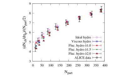
Figure 1: (Color Online) Charged-hadron multiplicity normalized by the number of the participant pair, $(dN_{\mathrm{ch}}/d\eta_{p})/(N_{\mathrm{part}}/2)$, as a function of the number of participants. The results from ideal hydrodynamics (open square), viscous hydrodynamics (open circle), fluctuating hydrodynamics–$\lambda 1.0$ (filled square), fluctuating hydrodynamics–$\lambda 1.5$ (filled circle), and fluctuating hydrodynamics–$\lambda 2.0$ (filled triangle) are compared with experimental data (open diamond) obtained by the ALICE Collaboration Aamodt et al. (2011b).

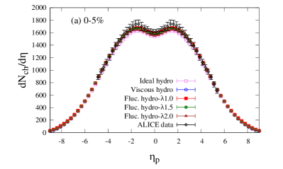
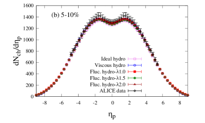
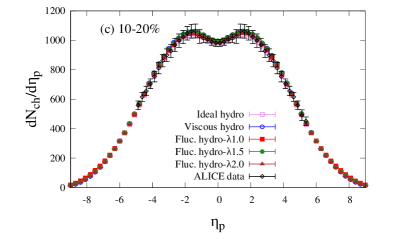
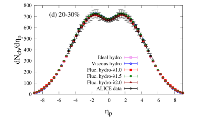
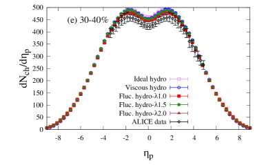
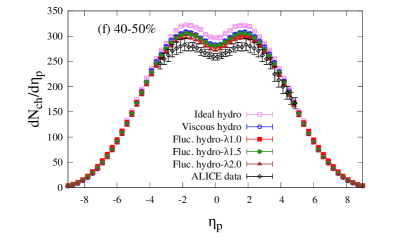
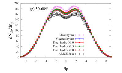
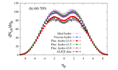
Figure 2: (Color Online) Pseudorapidity distributions of charged hadrons in Pb+Pb collisions at $\sqrt{s_{NN}}=2.76$ TeV. Centralities are (a) 0–5%, (b) 5–10%, (c) 10–20%, (d) 20–30%, (e) 30–40%, (f) 40–50%, (g) 50–60%, and (h) 60–70%. The symbols are the same as in Fig. 1. The experimental data are taken from Refs. Abbas et al. (2013); Adam et al. (2016).

Figures 2 (a)–(h) show the pseudorapidity dependence of charged-hadron multiplicity in Pb+Pb collisions at $\sqrt{s_{NN}}=2.76\ \text{TeV}$ for each centrality. Experimental data obtained by the ALICE Collaboration Abbas et al. (2013); Adam et al. (2016) are reproduced by all hydrodynamic models in a wide rapidity region in 0–30% centrality. The parameters $\sigma_{\eta}$ and $\Delta\eta$ control the shape of the distributions. We choose a single set of these parameters in each hydrodynamic model so as to reproduce experimental data in central collisions, which correspond to $N_{\mathrm{part}}\gtrsim 150$ in Fig. 1. Since we do not reproduce the centrality dependence of charged-hadron multiplicity at midrapidity below $N_{\mathrm{part}}\sim 150$ as shown in Fig. 1, pseudorapidity distributions are systematically larger than the experimental data in 30–70% regardless of the hydrodynamic models.

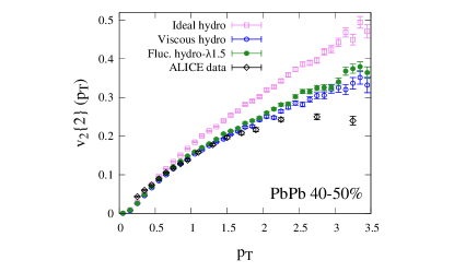
Figure 3: (Color Online) $v_{2}\{2\}(p_{T})$ in Pb+Pb collisions at $\sqrt{s_{NN}}=2.76\ \text{TeV}$ for centrality 40–50%. The results from ideal hydrodynamics (open square), viscous hydrodynamics (open circle), and fluctuating hydrodynamics–$\lambda 1.5$ (filled circle) are compared with experimental data (open diamond) obtained by the ALICE Collaboration Aamodt et al. (2010).

Figure 3 shows the transverse momentum ($p_{T}$) dependence of elliptic flow parameters $v_{2}\{2\}$ of charged hadrons in 40–50% central Pb+Pb collisions at $\sqrt{s_{NN}}=2.76\ \text{TeV}$. The elliptic flow parameters $v_{2}\{2\}\left(p_{T}\right)$ from the ideal hydrodynamic model is systematically larger than experimental data. Whereas, the shear viscosity suppresses $v_{2}\{2\}\left(p_{T}\right)$ in the viscous and the fluctuating hydrodynamic models. We reproduce the experimental data below $p_{T}=1.5\ \text{GeV}$ in the viscous and the fluctuating hydrodynamic models with $\eta/s=1/4\pi$. The elliptic flow parameters $v_{2}\{2\}\left(p_{T}\right)$ from the viscous and the fluctuating hydrodynamic models are almost the same with each other. This indicates that the hydrodynamic fluctuations do not affect $v_{2}\{2\}\left(p_{T}\right)$ apparently. Although hydrodynamic fluctuations are supposed to enhance fluctuations of elliptic flow parameters in general, its effect is not significant at this centrality. Note that we also obtain similar results of $v_{2}\{2\}\left(p_{T}\right)$ with the other values of $\lambda_{\perp}$ and $\lambda_{\eta}$ (not shown).

III.2 Factorization ratio

The hydrodynamic fluctuations disturb fluid evolution randomly in space and time according to Eq. (3). Therefore the correlations embedded in the initial longitudinal profiles such as alignment of participant-plane angles along space-time rapidity tend to be broken due to hydrodynamic fluctuations. To analyze such effects of the hydrodynamic fluctuations in the final state observables, we calculate the factorization ratios Gardim et al. (2013).

The factorization ratio in the longitudinal direction $r_{n}(\eta^{a}_{p},\eta^{b}_{p})$ is defined as

$$r_{n}(\eta^{a}_{p},\eta^{b}_{p}) =\frac{V_{n\Delta}(-\eta^{a}_{p},\eta^{b}_{p})}{V_{n\Delta}(\eta^{a}_{p},\eta^{b}_{p})},$$ (15)

$$V_{n\Delta}(\eta^{a}_{p},\eta^{b}_{p}) =\frac{\int\cos(n\Delta\phi)\frac{d^{2}N}{d\phi^{a}d\eta_{p}^{a}d\phi^{b}d\eta_{p}^{b}}d\phi^{a}d\phi^{b}}{\int\frac{d^{2}N}{d\phi^{a}d\eta_{p}^{a}d\phi^{b}d\eta_{p}^{b}}d\phi^{a}d\phi^{b}}.$$ (16)

Here $V_{n\Delta}(\eta^{a}_{p},\eta^{b}_{p})$ is the Fourier coefficient of two-particle azimuthal correlation functions at the $n$-th order. $\Delta\phi=\phi^{a}-\phi^{b}$ represents the difference of azimuthal angles between two charged hadrons. These two hadrons are taken from the two separated pseudorapidity, $\eta^{a}_{p}$ and $\eta^{b}_{p}$.

In the event-by-event calculations, the actual expression of $V_{n\Delta}(\eta^{a}_{p},\eta^{b}_{p})$ is given by

$$V_{n\Delta}(\eta^{a}_{p},\eta^{b}_{p}) =\langle\kern-1.0pt\langle{\cos(n\Delta\phi)}\rangle\kern-1.0pt\rangle=\frac{\Re\langle Q_{n}^{a*}Q_{n}^{b}\rangle}{\langle M^{a}M^{b}\rangle},$$ (17)

where $M^{a/b}$ and $Q_{n}^{a/b}=\sum_{i}e^{in\phi_{i}}$ are the multiplicity and the flow vector in the pseudorapidity bins at $\eta_{p}^{a/b}$ in a single event. The single angle brackets $\langle\cdots\rangle$ represent the average over the events at a given centrality, while the double angle brackets $\langle\kern-1.0pt\langle\cdots\rangle\kern-1.0pt\rangle$ represent the average over the particle pairs in each event in addition to the event average.

The factorization ratio (15) can be interpreted as the correlation between the flows in two pseudorapidity regions, $\eta^{a}_{p}$ and $-\eta^{a}_{p}$. Here the correlation of the event-plane angles (i.e., $\Psi_{n}^{a}$ and $\Psi_{n}^{-a}$) and that of the flow magnitudes (i.e., $v_{n}^{a}$ and $v_{n}^{-a}$) can be considered separately. The two-particle correlations $V_{n\Delta}$ (17) can be naively understood as

$$V_{n\Delta}(\eta^{a}_{p},\eta^{b}_{p})$$

$$\quad=\langle\kern-1.0pt\langle\cos\left[n(\phi^{a}-\phi^{b})\right]\rangle\kern-1.0pt\rangle$$

$$\quad=\langle\kern-1.0pt\langle\cos\{n\left[(\phi^{a}-\Psi_{n}^{a})-(\phi^{b}-\Psi_{n}^{b})+(\Psi_{n}^{a}-\Psi_{n}^{b})\right]\}\rangle\kern-1.0pt\rangle$$

$$\quad\approx\langle v_{n}^{a}v_{n}^{b}\cos[n(\Psi_{n}^{a}-\Psi_{n}^{b})]\rangle$$ (18)

by using the event-by-event flow magnitude $v_{n}^{a/b}=v_{n}(\eta_{p}^{a/b})$ and the event-plane angle $\Psi_{n}^{a/b}=\Psi_{n}(\eta^{a/b}_{p})$.

If we assume that the event-plane angles are completely aligned along rapidity, i.e., $\Psi_{n}^{a}=\Psi_{n}^{b}$, and also that the product of flow magnitudes at two different pseudorapidity regions factorized in the event averages, the two-particle correlations $V_{n\Delta}$ would be simplified:

$$V_{n\Delta}(\eta^{a}_{p},\eta^{b}_{p}) \approx\langle v_{n}^{a}v_{n}^{b}\rangle\approx\langle v_{n}^{a}\rangle\langle v_{n}^{b}\rangle.$$ (19)

In this ideal case, the factorization ratio becomes unity:

$$r_{n}(\eta^{a}_{p},\eta^{b}_{p})\approx\frac{\langle v_{n}^{-a}\rangle\langle v_{n}^{b}\rangle}{\langle v_{n}^{a}\rangle\langle v_{n}^{b}\rangle}=1,$$ (20)

since the flow magnitude is symmetric with respect to the pseudorapidity after averaging over all the events, i.e., $\langle v_{n}^{a}\rangle=\langle v_{n}^{-a}\rangle$, in symmetric systems like Pb+Pb collisions. However, the event-plane angle depends on pseudorapidity, therefore the two-particle correlations $V_{n\Delta}$ (III.2) cannot be factorized unlike in Eq. (19). Nevertheless, one still assumes the factorization among the flow magnitudes and the event-plane angles. In this case the two-particle correlation is written as

$$V_{n\Delta}(\eta^{a}_{p},\eta^{b}_{p}) \approx\langle v_{n}^{a}\rangle\langle v_{n}^{b}\rangle\langle\cos[n(\Psi_{n}^{a}-\Psi_{n}^{b})]\rangle.$$ (21)

Thus the factorization ratio has the following form:

$$r_{n}(\eta^{a}_{p},\eta^{b}_{p}) \approx\frac{\langle\cos[n(\Psi_{n}^{-a}-\Psi_{n}^{b})]\rangle}{\langle\cos[n(\Psi_{n}^{a}-\Psi_{n}^{b})]\rangle}<1.$$ (22)

The factorization ratio becomes smaller than unity since the event-plane angles are expected to be $(\Psi^{b}-\Psi^{-a})\geq(\Psi^{b}-\Psi^{a})$ on average due to the ordering of the rapidity gap $(\eta^{b}_{p}-\eta^{-a}_{p})\geq(\eta^{b}_{p}-\eta^{a}_{p})$. Therefore, the factorization ratio being smaller than unity implies that the event-plane angle depends on pseudorapidity.

Besides the event-plane angle decorrelation, asymmetry of the event-by-event flow magnitude also causes the factorization breakdown. Even if the event-plane angles are completely aligned, the two-particle correlations have an additional term coming from the correlation of the flow magnitude fluctuations:

$$V_{n\Delta}(\eta^{a}_{p},\eta^{b}_{p}) \approx\langle v_{n}^{a}v_{n}^{b}\rangle=\langle v_{n}^{a}\rangle\langle v_{n}^{b}\rangle+\langle\Delta v_{n}^{a}\Delta v_{n}^{b}\rangle,$$ (23)

where $\Delta v_{n}$ is the event-by-event flow magnitude fluctuations:

$$v_{n}=\langle v_{n}\rangle+\Delta v_{n}.$$ (24)

In this case, the factorization ratio becomes

$$r_{n}(\eta^{a}_{p},\eta^{b}_{p}) \approx\frac{\langle v_{n}^{-a}\rangle\langle v_{n}^{b}\rangle+\langle\Delta v_{n}^{-a}\Delta v_{n}^{b}\rangle}{\langle v_{n}^{a}\rangle\langle v_{n}^{b}\rangle+\langle\Delta v_{n}^{a}\Delta v_{n}^{b}\rangle}.$$ (25)

If the flow magnitude fluctuates asymmetrically in different pseudorapidity regions, $\langle\Delta v_{n}^{-a}\Delta v_{n}^{b}\rangle\leq\langle\Delta v_{n}^{a}\Delta v_{n}^{b}\rangle$ is expected due to the ordering of the rapidity gap. Thus the denominator becomes larger than the numerator in Eq. (25). Therefore the factorization ratio (25) becomes smaller than unity, $r_{n}(\eta^{a}_{p},\eta^{b}_{p})<1$, due to the reason similar to the case of the event-plane angle decorrelation in Eq. (22).

To summarize, the factorization ratio being smaller than unity indicates that the event-by-event rapidity decorrelation of the event-plane angle and/or the flow magnitude, i.e., the event-plane angle $\Psi_{n}$ and/or the flow magnitude $v_{n}$ depend on pseudorapidity in an event. Further discussions will be given in Sec. III.3 by introducing the Legendre coefficients to discriminate between the event-plane decorrelation and flow magnitude decorrelation.

In the following, $V_{n\Delta}(\eta^{a}_{p},\eta^{b}_{p})$ is calculated with the rapidity region $0<\eta^{a}_{p}<2.5$ and the transverse momentum region $0.3<p_{T}^{a}<3.0$ for a particle $a$, and the reference rapidity region $3.0<\eta^{b}_{p}<4.0$ for a particle $b$. These rapidity and transverse momentum regions follow the experimental setup of the CMS Collaboration Khachatryan et al. (2015).

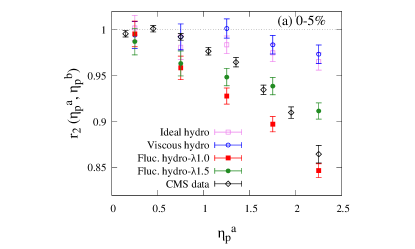
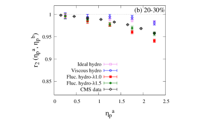
Figure 4: (Color Online) Factorization ratio in the longitudinal direction, $r_{2}(\eta^{a}_{p},\eta^{b}_{p})$, in Pb+Pb collisions at $\sqrt{s_{NN}}=2.76$ TeV for (a) 0–5% and (b) 20–30% centralities. The rapidity region for reference is $3.0<\eta_{p}^{b}<4.0$. The results from ideal hydrodynamics (open square), viscous hydrodynamics (open circle), fluctuating hydrodynamics–$\lambda 1.0$ (filled square) and fluctuating hydrodynamics–$\lambda 1.5$ (filled circle) are compared with experimental data (open diamond) obtained by the CMS Collaboration Khachatryan et al. (2015).

Figure 4 shows the factorization ratio in the longitudinal direction, $r_{2}(\eta^{a}_{p},\eta^{b}_{p})$, in Pb+Pb collisions at $\sqrt{s_{NN}}=2.76$ TeV for 0–5% and 20–30% centralities. The experimental data of $r_{2}(\eta^{a}_{p},\eta^{b}_{p})$ from the CMS Collaboration Khachatryan et al. (2015) is close to unity at small $\eta^{a}_{p}$ and decreases with increasing $\eta^{a}_{p}$. On the other hand, the factorization ratios $r_{2}(\eta^{a}_{p},\eta^{b}_{p})$ from the ideal and viscous hydrodynamic models modestly decrease with increasing $\eta^{a}_{p}$ in comparison with the experimental data, which means that expansion of the fluids tends to keep the long-range correlation in the rapidity direction. As discussed in Sec. II.2, the initial entropy distributions (8) are smooth functions of space-time rapidity and their transverse profile fluctuates due to the random positions of nucleons in colliding nuclei. In such a case, its participant-plane angles are almost the same for different space-time rapidities. Therefore, ideal and viscous hydrodynamic evolution directly translates longitudinal correlations in the initial profiles into correlations of the event-plane angle along pseudorapidity in final momentum anisotropy. It should be noted here that the small decorrelation in ideal and viscous hydrodynamic models is understood from the weak twist structure in the modified BGK model which is mentioned in Sec. II.2. In comparison with the results from the ideal and the viscous hydrodynamic models, the factorization ratios from the fluctuating hydrodynamic models are significantly smaller than unity at a large rapidity separation and are comparable with the experimental data. This indicates that hydrodynamic fluctuations break the factorization of the two-particle correlation function and cause rapidity decorrelation of the magnitude of anisotropic flow and/or the event-plane angle. Results from the fluctuating hydrodynamic models depend on the cutoff parameters in Eq. (7). Larger cutoff parameters correspond to smaller magnitudes of hydrodynamic fluctuations, and fluctuating hydrodynamics is reduced to the viscous hydrodynamics in the large limit of these parameters. The results shown in Fig. 4 are consistent with this perspective.

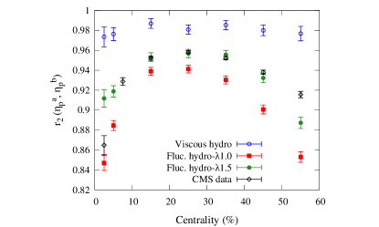
Figure 5: (Color Online) Centrality dependence of factorization ratio $r_{2}(\eta^{a}_{p},\eta^{b}_{p})$ in Pb+Pb collisions at $\sqrt{s_{NN}}=2.76$ TeV. The rapidity regions of two-particle correlation functions are taken as $2.0<\eta^{a}_{p}<2.5$ and $3.0<\eta^{b}_{p}<4.0$. The symbols are the same as in Fig. 4. The experimental data are taken from Ref. Khachatryan et al. (2015).

Figure 5 shows the centrality dependence of $r_{2}(\eta^{a}_{p},\eta^{b}_{p})$ in Pb+Pb collisions at $\sqrt{s_{NN}}=2.76$ TeV. The experimental data of $r_{2}(\eta^{a}_{p},\eta^{b}_{p})$ are smaller in the central collisions (0–10% centrality) and the peripheral collisions (50–60% centrality) than in the semi-central collisions (10–50% centrality). This is understood from the correlations embedded in the initial profiles. In the semi-central collisions, the initial geometry becomes elliptical to generate strong correlations of the participant-plane angle in the longitudinal direction. This initial correlation is reflected in the final momentum anisotropy, and the factorization ratio $r_{2}(\eta^{a}_{p},\eta^{b}_{p})$ tends to be close to unity in semi-central collisions. The factorization ratio $r_{2}(\eta^{a}_{p},\eta^{b}_{p})$ from the viscous hydrodynamic model is close to unity and this model fails to reproduce the experimental data for the whole centrality region. In contrast, $r_{2}(\eta^{a}_{p},\eta^{b}_{p})$ obtained from the fluctuating hydrodynamic models show qualitatively the same behavior as experimental data. In the central collisions (0–10% centrality), the fluctuating hydrodynamic model–$\lambda 1.0$ reproduces the experimental data reasonably well. Whereas, the fluctuating hydrodynamic model–$\lambda 1.5$ better reproduces the experimental data in the semi-central collisions (centrality classes between 10–50%). Therefore, the fluctuating hydrodynamic model could reproduce the experimental data of the centrality dependence of $r_{2}(\eta^{a}_{p},\eta^{b}_{p})$ by using a different set of the Gaussian width (i.e., $\lambda_{\perp}$ and $\lambda_{\eta}$) for a different centrality.

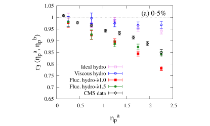
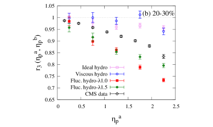
Figure 6: (Color Online) Factorization ratio $r_{3}(\eta^{a}_{p},\eta^{b}_{p})$ in Pb+Pb collisions at $\sqrt{s_{NN}}=2.76\ \text{TeV}$ for (a) 0–5% and (b) 20–30% centralities. The symbols are the same as in Fig. 4. The experimental data are taken from Ref. Khachatryan et al. (2015).

The second-order anisotropic flow (elliptic flow) is driven mainly by the initial geometry. In contrast, the third- (or, in general, odd-) order anisotropic flows are purely caused by fluctuations. The pattern of fluctuations in the initial transverse profile originating from the configuration of nucleons in the colliding nuclei is almost the same for different rapidities. The event-plane angles at the third order would also be correlated along pseudorapidity as in the case for elliptic flow. To suppress the effect of initial collision geometry on the factorization ratios and to see the effects of hydrodynamic fluctuations more directly, we also analyze $r_{3}(\eta^{a}_{p},\eta^{b}_{p})$. The third-order anisotropic flow (triangular flow) at a given pseudorapidity is generated from fluctuations of initial transverse profile at almost the same space-time rapidity. Figure 6 shows the factorization ratio $r_{3}(\eta^{a}_{p},\eta^{b}_{p})$ in Pb+Pb collisions at $\sqrt{s_{NN}}=2.76$ TeV for 0–5% and 20–30% centralities. The experimental data of $r_{3}(\eta^{a}_{p},\eta^{b}_{p})$ from the CMS Collaboration Khachatryan et al. (2015) decreases with increasing $\eta_{p}^{a}$. On the other hand, $r_{3}(\eta^{a}_{p},\eta^{b}_{p})$ from the viscous hydrodynamic model are close to unity and almost the same as those from the ideal hydrodynamic model. This indicates the viscosity itself does not further affect rapidity decorrelation of the third-order anisotropic flow. Whereas, hydrodynamic fluctuations reduce $r_{3}(\eta^{a}_{p},\eta^{b}_{p})$ considerably and it drops linearly with $\eta_{p}^{a}$. Although the experimental data of factorization ratio $r_{2}(\eta^{a}_{p},\eta^{b}_{p})$ are roughly reproduced with $\lambda_{\perp}=1.0$–$1.5\ \text{fm}$ in the fluctuating hydrodynamic model, $r_{3}(\eta^{a}_{p},\eta^{b}_{p})$ with the same setups are systematically smaller than the experimental data. Note that this is the opposite trend seen by the twist structure of the initial profiles in Ref. Bozek and Broniowski (2018) in which $r_{2}$ decorrelates too much while $r_{3}$ reproduces experimental data.

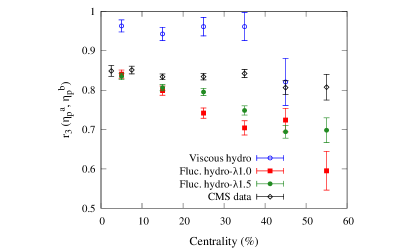
Figure 7: (Color Online) Centrality dependence of factorization ratio $r_{3}(\eta^{a}_{p},\eta^{b}_{p})$ in Pb+Pb collisions at $\sqrt{s_{NN}}=2.76$ TeV. The rapidity regions of two-particle correlation functions are taken as $2.0<\eta^{a}_{p}<2.5$ and $3.0<\eta^{b}_{p}<4.0$. The meaningful result for 50–60% centrality from viscous hydrodynamic model was not obtained due the insufficient statistics. The symbols are the same as in Fig. 4. The experimental data are taken from Ref. Khachatryan et al. (2015).

Figure 7 shows the centrality dependence of $r_{3}(\eta^{a}_{p},\eta^{b}_{p})$ in Pb+Pb collisions at $\sqrt{s_{NN}}=2.76$ TeV. The experimental data has almost no dependence on the centrality. Since Pb+Pb collision system is symmetric in rapidity, the longitudinal decorrelation of triangular flows purely comes from fluctuations. The factorization ratio $r_{3}(\eta^{a}_{p},\eta^{b}_{p})$ from the viscous hydrodynamic model is close to unity and this model fails to reproduce the experimental data in central collisions. In contrast, $r_{3}(\eta^{a}_{p},\eta^{b}_{p})$ obtained from the fluctuating hydrodynamic models reproduces the experimental data reasonably well in the central collisions (0–10% centrality). Whereas, $r_{3}(\eta^{a}_{p},\eta^{b}_{p})$ obtained from the fluctuating hydrodynamic models are smaller than the experimental data in the peripheral collisions (10–60% centralities).

III.3 Legendre coefficients

It is known that the effects of both the flow magnitude asymmetry and the event-plane twist reduce the factorization ratios Jia and Huo (2014). The original definition of the factorization ratio by CMS Khachatryan et al. (2015) cannot discriminate between the effects of the flow magnitude asymmetry and the event-plane twist. While, improved definitions of factorization ratios are proposed by ATLAS Aaboud et al. (2018) to discriminate between them by assuming the linear dependence of flow magnitude and event-plane angles. In addition to these two rapidity-decorrelation mechanisms, the analysis in the previous subsection reveals that hydrodynamic fluctuations also reduce the factorization ratios. In this subsection, we calculate the Legendre coefficients of the flow magnitude and the event-plane angle to separately estimate the effects of the flow magnitude asymmetry and the event-plane twist. The Legendre coefficients were previously used to quantify the longitudinal multiplicity fluctuations Monnai and Schenke (2016). We show that they can also be used to quantify the event-by-event longitudinal structure of the anisotropic flow parameter $v_{n}(\eta_{p})$ and the event-plane angle $\Psi_{n}(\eta_{p})$.

The pseudorapidity dependence of anisotropic flow $v_{n}$ and its event-plane angle $\Psi_{n}$ for each hydrodynamic event are expanded by using the Legendre polynomial $P_{k}$ as

$$v_{n}(\eta_{p}) =\sum_{k=0}^{\infty}a_{n}^{k}P_{k}\left(\frac{\eta_{p}}{\eta^{\mathrm{max}}_{p}}\right),$$ (26)

$$\Psi_{n}(\eta_{p}) =\sum_{k=0}^{\infty}b_{n}^{k}P_{k}\left(\frac{\eta_{p}}{\eta^{\mathrm{max}}_{p}}\right),$$ (27)

where $a_{n}^{k}$ and $b_{n}^{k}$ are the Legendre coefficients which measure the magnitude of the Legendre mode in the longitudinal direction for the flow parameters and event-plane angles, respectively. In particular, the magnitudes of $a_{n}^{1}$ and $b_{n}^{1}$ correspond to the anisotropic flow asymmetry and the event-plane twist Jia and Huo (2014), respectively.

These Legendre coefficients fluctuate from event to event due to the event-by-event twisted initial conditions and the hydrodynamic fluctuations. To obtain the magnitudes of these coefficients, we define the root mean square of the coefficients as

$$A_{n}^{k} =\sqrt{\langle(a_{n}^{k})^{2}\rangle_{\mathrm{ev}}}, B_{n}^{k} =\sqrt{\langle(b_{n}^{k})^{2}\rangle_{\mathrm{ev}}}.$$ (28)

Here $\langle\cdots\rangle_{\mathrm{ev}}$ represents the average over hydrodynamic events at a given centrality.

We calculate $v_{n}(\eta_{p})$ and $\Psi_{n}(\eta_{p})$ of each hydrodynamic event combining the final-state hadrons from all the oversampled cascade events. Thus we suppress the non-flow effects and the finite particle number effects in this analysis. We consider a rapidity range $|\eta_{p}|<\eta^{\mathrm{max}}_{p}=2.5$ which we used in the analysis of the factorization ratios. In the following, we consider up to $k=2$ and the first three Legendre polynomials are given as

$$P_{0}(x) =1, P_{1}(x) =x, P_{2}(x) =\frac{1}{2}(3x^{2}-1).$$ (29)

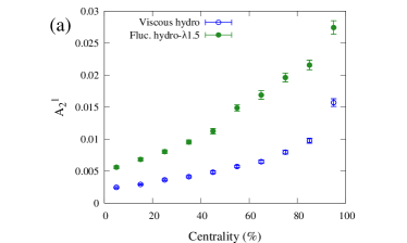
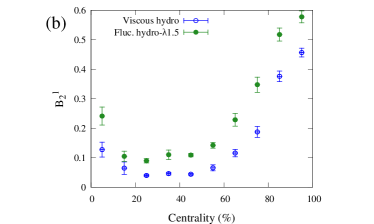
Figure 8: (Color Online) Centrality dependence of the first-order Legendre coefficients (a) $A^{1}_{2}$ and (b) $B^{1}_{2}$ for elliptic flow ($n=2$). The results from the viscous hydrodynamic model (open circle) and the fluctuating hydrodynamic model (filled circle) are shown for comparison.

Figure 8 shows the first-order Legendre coefficients $A^{1}_{2}$ and $B^{1}_{2}$ for elliptic flow ($n=2$) as functions of centrality from the viscous and the fluctuating hydrodynamic models. Both $A^{1}_{2}$ and $B^{1}_{2}$ from the fluctuating hydrodynamic model are systematically larger than the ones from the viscous hydrodynamic model. This implies that hydrodynamic fluctuations enhance a linear $\eta_{p}$-dependence of both the second-order anisotropic flow parameter $v_{2}$ and its event-plane angle $\Psi_{2}$ from event to event. The coefficient $B_{2}^{1}$ takes a minimum around 20–50% for both viscous and fluctuating hydrodynamics. This is because the event-plane angle is stabilized by the strong elliptical geometry of initial transverse profiles in the semi-central collisions. Therefore, the event-plane angle receives relatively smaller influences from the twist of the initial conditions and the hydrodynamic fluctuations. Meanwhile, the coefficient $A_{2}^{1}$ monotonically increases as a function of centrality percentile. This indicates that the development of the flow asymmetry in the longitudinal direction is independent of the transverse anisotropy driven by collision geometry. This increasing behavior of $A_{2}^{1}$ can be understood in the following way: The longitudinal asymmetries are originally introduced locally at each transverse position by the rapidity dependence of Eq. (8) and hydrodynamic fluctuations and then reflected in the observed flow by the matter evolution. When the transverse area of the created matter is large, such local asymmetry fluctuations are averaged out within the transverse plane so that the effect on the flow asymmetry fluctuations becomes relatively smaller. While, in the peripheral collisions, the local asymmetries can be directly reflected in the final flow asymmetry without the averaging effect. Thus, the magnitude of fluctuations becomes relatively larger in peripheral collisions.

Although the effects of the linear dependence of $v_{n}(\eta_{p})$ and $\Psi_{n}(\eta_{p})$ on the rapidity decorrelation have been discussed Jia and Huo (2014); Aaboud et al. (2018), discussion on the effects of the higher-order dependence is absent. From the non-linear behavior of the factorization ratio shown in the previous subsection, the higher-order dependence cannot be neglected in understanding the detailed mechanism of rapidity decorrelation. Therefore, we also calculate the second-order Legendre coefficients to quantify non-linear behaviors of the second-order anisotropic flow as a function of pseudorapidity.

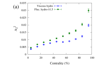
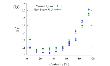
Figure 9: (Color Online) Centrality dependence of the second-order Legendre coefficients (a) $A^{2}_{2}$ and (b) $B^{2}_{2}$ for elliptic flow ($n=2$). The symbols are the same as in Fig. 8.

Figure 9 shows the second-order Legendre coefficients $A^{2}_{2}$ and $B^{2}_{2}$ for elliptic flow ($n=2$) as a function of centrality from the viscous and the fluctuating hydrodynamic models. $A^{2}_{2}$ from the fluctuating hydrodynamic model is systematically larger than the one from the viscous hydrodynamic model. $A^{2}_{2}$ from viscous hydrodynamics has a slight hump in centrality 30–50%, which can be understood from the large magnitude of $v_{2}$ in this centrality by considering the fact that the mode $A^{2}_{2}$ is due not only to the flow fluctuations but also to the average flow magnitude. While, $A^{2}_{2}$ monotonically increases with centrality percentile in the fluctuating hydrodynamic model, which implies the dominance of the flow fluctuations over the average flow magnitude. $B^{2}_{2}$ from viscous hydrodynamics and fluctuating hydrodynamics are both non-zero and even have a similar magnitude to the first-order coefficient $B_{2}^{1}$. In particular, $B^{2}_{2}$ are sizable in central (0–10%) and peripheral (60–100%) collisions. Since $B^{2}_{2}$ is the Legendre coefficient of the second-order Legendre polynomials, the event-plane angle is not only linear but quadratic as a function of pseudorapidity. This means that the event-by-event event-plane angle contains a rapidity-even component and that the twist direction of the event-plane rotation is not necessarily to be in one direction unlike in the twist case. This second-order mode is larger in central (0–10%) and peripheral (60–100%) than that in semi-central (10–60%) collisions. Similar to the first-order Legendre coefficients, this decrease of $B^{2}_{2}$ in semi-central collisions can be understood from the stabilized event plane due to the collision geometry.

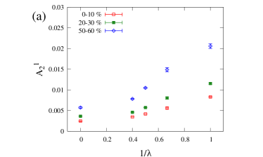
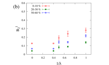
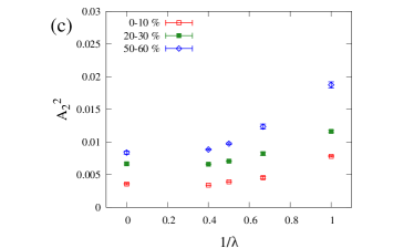
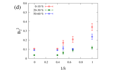
Figure 10: (Color Online) Cutoff parameter dependence of the Legendre coefficients. The first and the second-order Legendre coefficients for the magnitude and the event-plane angle of elliptic flow parameters, (a) $A^{1}_{2}$, (b) $A^{2}_{2}$, (c) $B^{1}_{2}$, and (d) $B^{2}_{2}$, from viscous hydrodynamics and fluctuating hydrodynamics–$\lambda 1.0$, $\lambda 1.5$, $\lambda 2.0$, and $\lambda 2.5$ are shown. The results from viscous hydrodynamics are plotted at $1/\lambda=0$ (or $\lambda=\infty$). The results are shown for centrality 0–10% (open square), 20–30% (filled square), and 50–60% (open diamond).

We analyze the cutoff parameter dependence of the Legendre coefficients to understand how much the hydrodynamic fluctuations affect the pseudorapidity dependences of the magnitude $v_{2}$ and the event-plane angle $\Psi_{2}$ of the second-order anisotropic flow parameters. Figure 10 shows the $1/\lambda$ dependence of the first- and second-order Legendre coefficients from the viscous and the fluctuating hydrodynamic models. Here the viscous hydrodynamic model can be regarded as a fluctuating hydrodynamic model with $\lambda=\infty$ (or $1/\lambda=0$). The magnitude of hydrodynamic fluctuations becomes larger with the smaller $\lambda$ so that the Legendre coefficients increase with decreasing $\lambda$ in Fig. 10. The coefficients for the magnitude, $A_{2}^{1}$ and $A_{2}^{2}$, are minimum in central collisions (0–10%) and increase with centrality percentile. On the other hand, the coefficient for the event-plane angle, $B_{2}^{1}$ and $B_{2}^{2}$, are minimum in centrality 20–30% and larger in central collisions (0–10%) and peripheral collisions (50–60%). This difference is due to the same reason discussed for Fig. 8. In particular, a monotonically increasing behavior of $A_{2}^{1}$ can also be seen in the second-order Legendre coefficient $A_{2}^{2}$. One sees that the values of the Legendre coefficients at $1/\lambda=0.4=1.0/2.5$ are already almost the same as the ones from the viscous hydrodynamics ($1/\lambda=0$) except for $A_{2}^{1}$. Therefore we conclude that hydrodynamic fluctuations become significant for the physics of the scale smaller than $\sim 2.0\ \text{fm}$.

IV Summary

We studied the effects of the hydrodynamic fluctuations during the evolution of the QGP fluids on rapidity decorrelation. We employed an integrated dynamical model in which the hydrodynamic model, rfh, implementing the causal hydrodynamic fluctuations and dissipations, is combined with the hadronic cascade model JAM. We performed simulations of Pb+Pb collisions at $\sqrt{s_{NN}}=2.76\ \text{TeV}$ using the integrated dynamical model. For comparison, we simulated the hydrodynamic stage with or without the hydrodynamic fluctuations and with different sets of the cutoff parameters ($\lambda_{\perp}$ and $\lambda_{\eta}$). We fixed the model parameters so that our model fairly reproduces the experimental data of the multiplicity normalized by the number of the participant, the pseudorapidity distributions, and the transverse momentum dependence of $v_{2}\{2\}$ for charged hadrons. With this model, we calculated the factorization ratio $r_{n}$ in the longitudinal direction and its centrality dependence to estimate the effects of hydrodynamic fluctuations on rapidity decorrelation. We found that the hydrodynamic fluctuations bring the sizable effects on the factorization ratios: Due to the nature of hydrodynamic fluctuations being random in space and time, longitudinal correlations of anisotropic flow tend to break down. To further understand this, we calculated the Legendre coefficients of the magnitude and the event-plane angle of anisotropic flow parameters that characterize the fluctuations of the longitudinal flow decorrelation. These Legendre coefficients increase by adding hydrodynamic fluctuations. We also analyzed the cutoff parameter dependence of the Legendre coefficients and found that the Legendre coefficients increase with larger $1/\lambda$ (smaller $\lambda$). These analyses showed that hydrodynamic fluctuations with a small cutoff parameter below $\lambda\sim 2$ play an important role in understanding rapidity decorrelation phenomena.

Although we found the significance of the hydrodynamic fluctuations in understanding longitudinal dynamics in high-energy nuclear collisions, we did not perfectly reproduce the pseudorapidity and the centrality dependences of the factorization ratios. In future, we plan to investigate the effects of initial fluctuations of longitudinal profiles which are missing in the present study. In particular, we will quantify how much the initial longitudinal fluctuations together with the hydrodynamic fluctuations bring the rapidity decorrelations in describing the factorization ratios.

Since the power of the fluctuating forces given by the FDR depends on temperature explicitly together with the shear viscous coefficient, the additional temperature dependence appears. Along the lines of this perspective, the collision energy dependence of the factorization ratios would be also interesting since the maximum temperature of the system created in heavy-ion collisions at the RHIC top energy would be smaller compared with the one at LHC. One could have a chance to focus more on the dynamics around the transition region ($T\sim 160$ MeV).

References

- Yagi et al. (2005) K. Yagi, T. Hatsuda, and Y. Miake, Camb. Monogr. Part. Phys. Nucl. Phys. Cosmol. 23, 1 (2005).
- Ollitrault (1992) J.-Y. Ollitrault, Phys. Rev. D46, 229 (1992).
- Ackermann et al. (2001) K. H. Ackermann et al. (STAR), Phys. Rev. Lett. 86, 402 (2001), arXiv:nucl-ex/0009011 [nucl-ex] .
- Adler et al. (2001) C. Adler et al. (STAR), Phys. Rev. Lett. 87, 182301 (2001), arXiv:nucl-ex/0107003 [nucl-ex] .
- Adams et al. (2004) J. Adams et al. (STAR), Phys. Rev. Lett. 92, 052302 (2004), arXiv:nucl-ex/0306007 [nucl-ex] .
- Adcox et al. (2002) K. Adcox et al. (PHENIX), Phys. Rev. Lett. 89, 212301 (2002), arXiv:nucl-ex/0204005 [nucl-ex] .
- Adler et al. (2003) S. S. Adler et al. (PHENIX), Phys. Rev. Lett. 91, 182301 (2003), arXiv:nucl-ex/0305013 [nucl-ex] .
- Back et al. (2002) B. B. Back et al. (PHOBOS), Phys. Rev. Lett. 89, 222301 (2002), arXiv:nucl-ex/0205021 [nucl-ex] .
- Kolb et al. (2001) P. F. Kolb, P. Huovinen, U. W. Heinz, and H. Heiselberg, Phys. Lett. B500, 232 (2001), arXiv:hep-ph/0012137 [hep-ph] .
- Huovinen et al. (2001) P. Huovinen, P. F. Kolb, U. W. Heinz, P. V. Ruuskanen, and S. A. Voloshin, Phys. Lett. B503, 58 (2001), arXiv:hep-ph/0101136 [hep-ph] .
- Teaney et al. (2001a) D. Teaney, J. Lauret, and E. V. Shuryak, Phys. Rev. Lett. 86, 4783 (2001a), arXiv:nucl-th/0011058 [nucl-th] .
- Teaney et al. (2001b) D. Teaney, J. Lauret, and E. V. Shuryak, (2001b), arXiv:nucl-th/0110037 [nucl-th] .
- Hirano (2002) T. Hirano, Phys. Rev. C65, 011901 (2002), arXiv:nucl-th/0108004 [nucl-th] .
- Hirano and Tsuda (2002) T. Hirano and K. Tsuda, Phys. Rev. C66, 054905 (2002), arXiv:nucl-th/0205043 [nucl-th] .
- Heinz and Kolb (2002) U. W. Heinz and P. F. Kolb, Statistical QCD. Proceedings, International Symposium, Bielefeld, Germany, August 26-30, 2001, Nucl. Phys. A702, 269 (2002), arXiv:hep-ph/0111075 [hep-ph] .
- Lee (2005) T. D. Lee, Quark gluon plasma. New discoveries at RHIC: A case of strongly interacting quark gluon plasma. Proceedings, RBRC Workshop, Brookhaven, Upton, USA, May 14-15, 2004, Nucl. Phys. A750, 1 (2005).
- Gyulassy and McLerran (2005) M. Gyulassy and L. McLerran, Quark gluon plasma. New discoveries at RHIC: A case of strongly interacting quark gluon plasma. Proceedings, RBRC Workshop, Brookhaven, Upton, USA, May 14-15, 2004, Nucl. Phys. A750, 30 (2005), arXiv:nucl-th/0405013 [nucl-th] .
- Shuryak (2005) E. V. Shuryak, Quark gluon plasma. New discoveries at RHIC: A case of strongly interacting quark gluon plasma. Proceedings, RBRC Workshop, Brookhaven, Upton, USA, May 14-15, 2004, Nucl. Phys. A750, 64 (2005), arXiv:hep-ph/0405066 [hep-ph] .
- Hirano and Gyulassy (2006) T. Hirano and M. Gyulassy, Nucl. Phys. A769, 71 (2006), arXiv:nucl-th/0506049 [nucl-th] .
- Aamodt et al. (2010) K. Aamodt et al. (ALICE), Phys. Rev. Lett. 105, 252302 (2010), arXiv:1011.3914 [nucl-ex] .
- Chatrchyan et al. (2011) S. Chatrchyan et al. (CMS), JHEP 08, 141 (2011), arXiv:1107.4800 [nucl-ex] .
- Aad et al. (2012a) G. Aad et al. (ATLAS), Phys. Lett. B707, 330 (2012a), arXiv:1108.6018 [hep-ex] .
- Adare et al. (2011) A. Adare et al. (PHENIX), Phys. Rev. Lett. 107, 252301 (2011), arXiv:1105.3928 [nucl-ex] .
- Adam et al. (2019) J. Adam et al. (STAR), Phys. Rev. Lett. 122, 172301 (2019), arXiv:1901.08155 [nucl-ex] .
- Aamodt et al. (2011a) K. Aamodt et al. (ALICE), Phys. Rev. Lett. 107, 032301 (2011a), arXiv:1105.3865 [nucl-ex] .
- Aad et al. (2012b) G. Aad et al. (ATLAS), Phys. Rev. C86, 014907 (2012b), arXiv:1203.3087 [hep-ex] .
- Chatrchyan et al. (2012) S. Chatrchyan et al. (CMS), Eur. Phys. J. C72, 2012 (2012), arXiv:1201.3158 [nucl-ex] .
- Alver and Roland (2010) B. Alver and G. Roland, Phys. Rev. C81, 054905 (2010), [Erratum: Phys. Rev.C82,039903(2010)], arXiv:1003.0194 [nucl-th] .
- Song and Heinz (2008) H. Song and U. W. Heinz, Phys. Rev. C77, 064901 (2008), arXiv:0712.3715 [nucl-th] .
- Dusling and Teaney (2008) K. Dusling and D. Teaney, Phys. Rev. C77, 034905 (2008), arXiv:0710.5932 [nucl-th] .
- Luzum and Romatschke (2008) M. Luzum and P. Romatschke, Phys. Rev. C78, 034915 (2008), [Erratum: Phys. Rev.C79,039903(2009)], arXiv:0804.4015 [nucl-th] .
- Schenke et al. (2010) B. Schenke, S. Jeon, and C. Gale, Phys. Rev. C82, 014903 (2010), arXiv:1004.1408 [hep-ph] .
- Bozek et al. (2011a) P. Bozek, M. Chojnacki, W. Florkowski, and B. Tomasik, Phys. Lett. B694, 238 (2011a), arXiv:1007.2294 [nucl-th] .
- Song et al. (2011a) H. Song, S. A. Bass, U. Heinz, T. Hirano, and C. Shen, Phys. Rev. Lett. 106, 192301 (2011a), [Erratum: Phys. Rev. Lett.109,139904(2012)], arXiv:1011.2783 [nucl-th] .
- Song et al. (2011b) H. Song, S. A. Bass, and U. Heinz, Phys. Rev. C83, 054912 (2011b), [Erratum: Phys. Rev.C87,no.1,019902(2013)], arXiv:1103.2380 [nucl-th] .
- Schenke et al. (2011) B. Schenke, S. Jeon, and C. Gale, Phys. Lett. B702, 59 (2011), arXiv:1102.0575 [hep-ph] .
- Bernhard et al. (2016) J. E. Bernhard, J. S. Moreland, S. A. Bass, J. Liu, and U. Heinz, Phys. Rev. C94, 024907 (2016), arXiv:1605.03954 [nucl-th] .
- Bernhard et al. (2019) J. E. Bernhard, J. S. Moreland, and S. A. Bass, Nature Phys. 15, 1113 (2019).
- Calzetta (1998) E. Calzetta, Class. Quant. Grav. 15, 653 (1998), arXiv:gr-qc/9708048 [gr-qc] .
- Kapusta et al. (2012) J. I. Kapusta, B. Muller, and M. Stephanov, Phys. Rev. C85, 054906 (2012), arXiv:1112.6405 [nucl-th] .
- Murase and Hirano (2013) K. Murase and T. Hirano, (2013), arXiv:1304.3243 [nucl-th] .
- Murase and Hirano (2016) K. Murase and T. Hirano, Proceedings, 25th International Conference on Ultra-Relativistic Nucleus-Nucleus Collisions (Quark Matter 2015): Kobe, Japan, September 27-October 3, 2015, Nucl. Phys. A956, 276 (2016), arXiv:1601.02260 [nucl-th] .
- Murase (2015) K. Murase, Causal hydrodynamic fluctuations and their effects on high-energy nuclear collisions, Ph.D. thesis, The University of Tokyo (2015).
- Murase (2019) K. Murase, Annals Phys. 411, 167969 (2019), arXiv:1904.11217 [nucl-th] .
- Akamatsu et al. (2017) Y. Akamatsu, A. Mazeliauskas, and D. Teaney, Phys. Rev. C95, 014909 (2017), arXiv:1606.07742 [nucl-th] .
- Akamatsu et al. (2018) Y. Akamatsu, A. Mazeliauskas, and D. Teaney, Phys. Rev. C97, 024902 (2018), arXiv:1708.05657 [nucl-th] .
- Martinez, M. and Schäfer, Thomas (2019) Martinez, M. and Schäfer, Thomas, Phys. Rev. C99, 054902 (2019), arXiv:1812.05279 [hep-th] .
- An et al. (2019) X. An, G. Basar, M. Stephanov, and H.-U. Yee, Phys. Rev. C100, 024910 (2019), arXiv:1902.09517 [hep-th] .
- Gardim et al. (2013) F. G. Gardim, F. Grassi, M. Luzum, and J.-Y. Ollitrault, Phys. Rev. C87, 031901 (2013), arXiv:1211.0989 [nucl-th] .
- Khachatryan et al. (2015) V. Khachatryan et al. (CMS), Phys. Rev. C92, 034911 (2015), arXiv:1503.01692 [nucl-ex] .
- Aaboud et al. (2018) M. Aaboud et al. (ATLAS), Eur. Phys. J. C78, 142 (2018), arXiv:1709.02301 [nucl-ex] .
- Huo (2017) P. Huo (ATLAS), Proceedings, 26th International Conference on Ultra-relativistic Nucleus-Nucleus Collisions (Quark Matter 2017): Chicago, Illinois, USA, February 5-11, 2017, Nucl. Phys. A967, 908 (2017).
- Nie (2019) M. Nie (STAR), Proceedings, 27th International Conference on Ultrarelativistic Nucleus-Nucleus Collisions (Quark Matter 2018): Venice, Italy, May 14-19, 2018, Nucl. Phys. A982, 403 (2019).
- Aad et al. (2020) G. Aad et al. (ATLAS), (2020), arXiv:2001.04201 [nucl-ex] .
- Bozek and Broniowski (2018) P. Bozek and W. Broniowski, Phys. Rev. C97, 034913 (2018), arXiv:1711.03325 [nucl-th] .
- Bozek et al. (2011b) P. Bozek, W. Broniowski, and J. Moreira, Phys. Rev. C83, 034911 (2011b), arXiv:1011.3354 [nucl-th] .
- Wu et al. (2018) X.-Y. Wu, L.-G. Pang, G.-Y. Qin, and X.-N. Wang, Phys. Rev. C98, 024913 (2018), arXiv:1805.03762 [nucl-th] .
- Jia et al. (2017) J. Jia, P. Huo, G. Ma, and M. Nie, J. Phys. G44, 075106 (2017), arXiv:1701.02183 [nucl-th] .
- Bozek and Broniowski (2016) P. Bozek and W. Broniowski, Phys. Lett. B752, 206 (2016), arXiv:1506.02817 [nucl-th] .
- Pang et al. (2015) L.-G. Pang, G.-Y. Qin, V. Roy, X.-N. Wang, and G.-L. Ma, Phys. Rev. C91, 044904 (2015), arXiv:1410.8690 [nucl-th] .
- Pang et al. (2016) L.-G. Pang, H. Petersen, G.-Y. Qin, V. Roy, and X.-N. Wang, Eur. Phys. J. A52, 97 (2016), arXiv:1511.04131 [nucl-th] .
- Pang et al. (2018) L.-G. Pang, H. Petersen, and X.-N. Wang, Phys. Rev. C97, 064918 (2018), arXiv:1802.04449 [nucl-th] .
- Schenke and Schlichting (2016) B. Schenke and S. Schlichting, Phys. Rev. C94, 044907 (2016), arXiv:1605.07158 [hep-ph] .
- Shen, Chun and Schenke, Björn (2018) Shen, Chun and Schenke, Björn, Phys. Rev. C97, 024907 (2018), arXiv:1710.00881 [nucl-th] .
- Behera et al. (2020) A. Behera, M. Nie, and J. Jia, (2020), arXiv:2003.04340 [nucl-th] .
- Hirano et al. (2013) T. Hirano, P. Huovinen, K. Murase, and Y. Nara, Progress in Particle and Nuclear Physics 70, 108 (2013).
- Hirano et al. (2006) T. Hirano, U. W. Heinz, D. Kharzeev, R. Lacey, and Y. Nara, Phys. Lett. B636, 299 (2006), arXiv:nucl-th/0511046 [nucl-th] .
- Nara et al. (2000) Y. Nara, N. Otuka, A. Ohnishi, K. Niita, and S. Chiba, Phys. Rev. C61, 024901 (2000), arXiv:nucl-th/9904059 [nucl-th] .
- Huovinen and Petreczky (2010) P. Huovinen and P. Petreczky, Nucl. Phys. A837, 26 (2010), arXiv:0912.2541 [hep-ph] .
- Glauber (2006) R. J. Glauber, Nucl. Phys. A774, 3 (2006).
- Brodsky et al. (1977) S. J. Brodsky, J. F. Gunion, and J. H. Kuhn, Phys. Rev. Lett. 39, 1120 (1977).
- Adil and Gyulassy (2005) A. Adil and M. Gyulassy, Phys. Rev. C72, 034907 (2005), arXiv:nucl-th/0505004 [nucl-th] .
- Bjorken (1983) J. D. Bjorken, Phys. Rev. D27, 140 (1983).
- Cooper and Frye (1974) F. Cooper and G. Frye, Phys. Rev. D10, 186 (1974).
- Teaney (2003) D. Teaney, Phys. Rev. C68, 034913 (2003), arXiv:nucl-th/0301099 [nucl-th] .
- Monnai and Hirano (2009) A. Monnai and T. Hirano, Phys. Rev. C80, 054906 (2009), arXiv:0903.4436 [nucl-th] .
- Kovtun et al. (2005) P. Kovtun, D. T. Son, and A. O. Starinets, Phys. Rev. Lett. 94, 111601 (2005), arXiv:hep-th/0405231 [hep-th] .
- Song (2009) H. Song, Causal Viscous Hydrodynamics for Relativistic Heavy Ion Collisions, Ph.D. thesis, Ohio State U. (2009), arXiv:0908.3656 [nucl-th] .
- Baier et al. (2008) R. Baier, P. Romatschke, D. T. Son, A. O. Starinets, and M. A. Stephanov, JHEP 04, 100 (2008), arXiv:0712.2451 [hep-th] .
- Aamodt et al. (2011b) K. Aamodt et al. (ALICE), Phys. Rev. Lett. 106, 032301 (2011b), arXiv:1012.1657 [nucl-ex] .
- Abbas et al. (2013) E. Abbas et al. (ALICE), Phys. Lett. B726, 610 (2013), arXiv:1304.0347 [nucl-ex] .
- Adam et al. (2016) J. Adam et al. (ALICE), Phys. Lett. B754, 373 (2016), arXiv:1509.07299 [nucl-ex] .
- Jia and Huo (2014) J. Jia and P. Huo, Phys. Rev. C90, 034905 (2014), arXiv:1402.6680 [nucl-th] .
- Monnai and Schenke (2016) A. Monnai and B. Schenke, Phys. Lett. B752, 317 (2016), arXiv:1509.04103 [nucl-th] .