Long-range Rydberg molecule Rb₂: Two-electron R-matrix calculations at intermediate internuclear distances

Abstract

The adiabatic potential energy curves of Rb₂ in the long-range Rydberg electronic states are calculated using the two-electron R-matrix method [M. Tarana, R. Čurík, Phys. Rev. A 93, 012515 (2016)] for the intermediate internuclear separations between 37 a.u. and 200 a.u. The results are compared with the zero-range models to find a region of the internuclear distances where the Fermi’s pseudopotential approach provides accurate energies. A finite-range potential model of the atomic perturber is used to calculate the wave functions of the Rydberg electron and their features specific for the studied range of internuclear distances are identified.

I Introduction

Diatomic long-range Rydberg molecule (LRRM) is an exotic system of two atoms – one in its ground state and one in its high excited state (typically $n\sim 10-80$), bound to each other at the distances of the nuclei varying between tens and thousands of Bohr radii. The mechanism of this bond consists in the scattering of the Rydberg electron off the distant neutral atom (perturber). This interaction can affect the phase of the Rydberg wave function in such way that the molecular electronic bound state is formed. When its energy, as a function of the internuclear distance, forms sufficiently deep well, the vibrational states of the LRRMs can be bound.

Existence of the LRRMs was first theoretically predicted by Greene et al. [1] almost two decades ago along with their unusually large permanent electric dipole moments, even for the homonuclear diatomic molecules. Two categories of the electronic bound states were identified: Those formed by the perturbation of the non-degenerate atomic Rydberg states with low angular momenta and the trilobite states involving the hydrogen-like degenerate atomic states with high angular momenta. It took almost nine years since then until the first experimental evidence of the LRRMs was provided by Bendkowsky et al. [2] and their electric dipole moment measured by Li et al. [3].

Since then, the LRRMs became a subject of intensive theoretical and experimental research. The trilobite-like states were observed in cesium by Booth et al. [4]. The existence of the butterfly states, predominated by the $p$-wave interaction of the Rydberg electron with the neutral perturber, predicted by Hamilton et al. [5], was experimentally confirmed by Niederprüm et al. [6]. The LRRMs have been so far predominately prepared in the ultracold atomic ensembles of the heavy alkali metals [2, 4, 6]. However, DeSalvo et al. [7], and more recently Ding et al. [8], reported successful creation of the LRRMs in the ultra-cold strontium gas.

The LRRMs have also provided ways to explore other phenomena. Schmid et al. [9] proposed an experiment where the ionized LRRM Li₂ provides a well defined initial state for the Li-Li⁺ collision in the quantum regime that was not available to previously developed experimental techniques. The LRRMs Rb₂ have also been utilized to study the effects of the spin-orbit interactions in the electron collisions with the rubidium atom at low scattering energies [10, 11].

Summary of the related research exceeds the scope of this article. For comprehensive review, see the recent papers [12, 13, 14] and references therein.

The first and so far most frequently utilized theoretical model of the LRRMs is based on the representation of the neutral perturber by the Fermi’s zero-range pseudo-potential [1, 5] that couples the atomic eigenstates of the Rydberg electron. This delta-function interaction possesses a singularity at the position of the perturber. It is usually considered non-zero only in the partial waves $s$ and $p$ and parameterized by the generalized energy-dependent electron-perturber scattering length [1, 15] in the $s$-wave. Following Omont [16], the $p$-wave component, particularly important for the alkali metals supporting the low-energy ${}^{3}P^{o}$ resonance, is parameterized by the low-energy $p$-wave phase shift of the electron-perturber scattering [5]. This simple model was more recently enhanced by taking the spin effects into account [17, 18] and provided an insight into several experimental results.

The computational method beyond the level of the perturbation theory, frequently employed to calculate the potential energy curves (PECs) of the zero-range model, is based on the diagonalization of the corresponding Hamiltonian in the finite basis set of the unperturbed atomic Rydberg states. This approach is associated with the issue that the eigenenergies do not converge with the increasing number of the Rydberg manifolds included in the basis set [19]. Another complication inherent to this method is the selection of the kinetic energies at which the scattering lengths are taken. The classical kinetic energy of the Rydberg electron at the position of the perturber, that determines their interaction in the zero-range model, depends on the total energy of the molecular electronic state. This is, however, not known at the stage of the computation when the Hamiltonian matrix is constructed. An alternative approach to the direct diagonalization of the zero-range Hamiltonian in the finite basis set of the atomic Rydberg states is the solution of the integral equation involving corresponding Green’s function [19].

The first study where the neutral perturber was represented by a finite-range potential, was due to Khuskivadze et al. [20]. This interaction was, similarly to the zero-range Fermi’s pseudopotential, optimized to correctly reproduce the phase shifts of the electron collisions with the atomic perturber.

The most frequently utilized experimental technique to prepare the LRRMs is their photoassociation in the ultra-cold atomic ensemble via excitation of the atoms into the Rydberg states (see the review by Shaffer et al. [13] and references therein). The involved atomic states typically possess the principal quantum numbers $n>30$ and corresponding relevant internuclear distances lie above 200 a.u. [13] where the Fermi’s zero-range model provides quantitatively satisfactory accuracy of the calculated electronic and vibrational energies.

However, Bellos et al. [21] carried out an experiment in which different mechanism was utilized to prepare the LRRMs Rb₂: First, weakly bound Rb₂ molecules in their lowest excited electronic and high vibrational state $\Ket{a^{3}\Sigma_{u}^{+},\,\nu=35}$ were photo-associated in the magneto-optical trap containing ultra-cold rubidium atoms. The LRRMs with the energies between the states $5s+7p$ and $5s+12p$ (in the asymptotic limit of the separated atoms) were then directly photo-excited. The information about the populations of different electronic and vibrational energy levels of the LRRMs was retrieved using the autoionization spectroscopy of the molecular cations Rb${}_{2}^{+}$. Later, the states slightly red-shifted with respect to the $5s+7p$ energy were studied in more detail by Carollo et al. [22].

The outer vibrational turning point of the initial molecular state $\Ket{a^{3}\Sigma_{u}^{+},\,\nu=35}$ is approximately at the internuclear separation $\approx 35$ a.u. and relatively low Rydberg energies are populated by the subsequent photo-excitation. As a result, the LRRMs prepared by Bellos et al. [21] possess significantly lower internuclear separations than those produced via the direct photo-association of the atomic pair utilized in majority of other experiments.

Although Bellos et al. [21] successfully associated some of the features observed in their experimental spectra with the structures in the PECs calculated using the Fermi’s pseudo-potentials [1, 5], the validity of this model becomes questionable at these small internuclear separations and low energies. Since the size of the perturber is not negligible compared to its distance from the Rydberg atomic core, their mutual interaction may become relevant. Similarly, the size of the perturber is not negligible compared to the de Broglie wave length of the Rydberg electron.

In order to address the validity of the zero-range model of the LRRMs at small internuclear distances, this article is dealing with the PECs of Rb₂ calculated using different models. The calculations are focused on the intermediate range of the internuclear separations below 200 a.u., similar to that studied by Bellos et al. [21]. A more advanced approach, suitable for this range of the nuclear distances, where the valence electron of the alkali-metal atomic perturber is explicitly represented as well as the Rydberg electron, was formulated by Tarana and Čurík [23] (hereafter referred to as TC). The construction of this model for Rb₂ is discussed in the present article along with the comparison between the obtained PECs and those published by Bellos et al. [21] to establish the range of the internuclear distances where the zero-range model provides quantitatively accurate results.

The two-electron R-matrix approach does not utilize any external parametrization of the interaction between the Rydberg electron and neutral perturber that depends on the kinetic energy of the electron. Instead, the solutions of the two-electron Schrödinger equation are calculated in the vicinity of the perturber affected by the positive Rydberg core. These are, in terms of the logarithmic derivative, smoothly matched to the wave functions calculated farther from the perturber that satisfy the bound-state asymptotic boundary conditions.

This paper presents the first application of the two-electron R-matrix approach [23] to other molecular system than H₂. Another goal of this work is to present the PECs associated with the perturber in its excited state as these exist below the ionization energy in Rb₂ and can be calculated using the approach developed in TC.

The probability densities of the Rydberg electron are also presented in terms of a one-particle finite-range model of the LRRMs [20] in order to understand their features that are specific to the range of the distances between the nuclei studied in this work.

The spin-orbit couplings and spin-spin couplings are not considered in the calculations presented here. Although their effects can be experimentally recognized in the heavy alkali metals [11, 13, 14], the phenomena investigated in this article are not directly related to the relativistic effects. Adding corresponding degrees of freedom to the two-electron R-matrix method formulated in TC would, for the study presented here, yield computationally more demanding calculations without providing equivalent additional insight into the underlying mechanisms.

The rest of this article is organized as follows: The essentials of the two-electron R-matrix theory of the LRRMs are reviewed in Section II. Sections III and IV are dealing with the parameters of the two-electron and one-electron R-matrix calculations, respectively. The results of the calculations are analyzed in Sections V and VI. The conclusions are formulated in Section VII. The model potential of Rb⁺ and corresponding quantum defects are discussed in Supplemental Material.

Unless explicitly stated otherwise, the atomic units are used throughout the rest of this article.

II Summary of two-electron R-matrix method

Only the essential elements of the two-electron R-matrix method are summarized in this section. For its detailed description, an interested reader is referred to the paper TC. Following the notation used in TC, the core of the perturber and the Rydberg core are denoted by $A$ and $B$, respectively.

The Rydberg electron is explicitly represented in the model as well as the valence electron of the perturber. The center of the coordinate system is located on the nucleus of the perturber, the Rydberg core is located on the $z$-axis. The coordinates of the electrons are denoted by $\mathbf{r}_{1}$ and $\mathbf{r}_{2}$, the position of the positive Rydberg core $B$ is denoted by $\mathbf{R}$ ($R$ is the internuclear separation). The radial coordinate of $\mathbf{r}_{i}$ is $r_{i}$ and $\Omega_{i}$ is used for the corresponding angular component.

The Hamiltonian of this system is

$$\hat{H}=\sum_{p=1,2}\left[\hat{K}_{p}+V_{A}(r_{p})+V_{B}(\left|\mathbf{r}_{p}-\mathbf{R}\right|)\right]+\frac{1}{r_{12}},$$ (1)

where $\hat{K}_{p}=-(1/2)\Delta$ is the kinetic-energy operator of the $p$-th electron, $V_{A}(r)$ and $V_{B}(r)$ are the potentials representing the positive cores $A$ and $B$, respectively. The last term is the repulsion between the Rydberg and valence electron. The interaction of the nuclei $1/R$ is a constant that is added to the final calculated energies and it skipped from all the equations for the brevity of the notation. Corresponding time-independent Schrödinger equation for a fixed internuclear distance $R$ reads

$$\hat{H}\Psi(\mathbf{r}_{1},\mathbf{r}_{2})=E\Psi(\mathbf{r}_{1},\mathbf{r}_{2}),$$ (2)

where $\Psi(\mathbf{r}_{1},\mathbf{r}_{2})$ is the two-electron bound-state wave function and $E$ denotes the corresponding eigenenergy. Projection of the total angular momentum $M=m_{1}+m_{2}$ on the nuclear axis is conserved. The projections of the single-electron angular momenta on the nuclear axis are denoted by $m_{1}$ and $m_{2}$.

The valence electron is located exclusively in the vicinity of the perturber core $A$ and only the Rydberg electron can appear in the remaining space. A sphere $\mathcal{S}$ centered on the core $A$ is introduced with radius $r_{0}<R$ and large enough to confine all the region where the probability density of the valence electron does not vanish. Then it is sufficient to treat the complicated two-electron Schrödinger equation only in the relatively small inner region and to smoothly match its solutions on the sphere to the single-particle wave functions calculated in the outer region.

II.1 Outer region

When the Rydberg electron is located in the outer region, the solution $\left.\Psi(\mathbf{r}_{1},\mathbf{r}_{2})\right|_{r_{2}\geq r_{0}}$ can be expressed using the bound states $\varphi_{im_{1}}(\mathbf{r}_{1})$ of the valence electron weakly affected by the Coulomb tail of $V_{B}(\left|\mathbf{r}_{1}-\mathbf{R}\right|)$ defined by the equation

$$\left[\hat{K}_{1}+V_{A}(r_{1})+V_{B}(\left|\mathbf{r}_{1}-\mathbf{R}\right|)\right] \varphi_{im_{1}}(\mathbf{r}_{1})$$

$$=\epsilon_{im_{1}} \varphi_{im_{1}}(\mathbf{r}_{1})$$ , (3a)

$$\left.\varphi_{im_{1}}(\mathbf{r}_{1})\right|_{r_{1}\geq r_{0}}\equiv 0,$$ (3b)

where $i$ indexes the bound states of the valence electron and $\epsilon_{im_{1}}$ are the corresponding discrete energies. Using these states, the total two-electron wave function $\left.\Psi(\mathbf{r}_{1},\mathbf{r}_{2})\right|_{r_{2}\geq r_{0}}$ can be expressed as

$$\left.\Psi(\mathbf{r}_{1},\mathbf{r}_{2})\right|_{r_{2}\geq r_{0}}=\sum_{im_{1}}\varphi_{im_{1}}(\mathbf{r}_{1})X_{im_{1}}(\mathbf{r}_{2}).$$ (4)

Projection of the Schrödinger equation (2) on the states $\varphi_{im_{1}}(\mathbf{r}_{1})$, along with the assumption that the interaction between the Rydberg electron and the perturber can be neglected in the outer region $\left[V_{A}(r\geq r_{0})\equiv 0\right]$, yields the following uncoupled set of the equations:

$$\left[\hat{K}_{2}+V_{B}(\left|\mathbf{r}_{2}-\mathbf{R}\right|)-(E-\epsilon_{im_{1}})\right]X_{im_{1}}(\mathbf{r}_{2})=0.$$ (5)

Introducing the spherical harmonics $Y_{lm}(\Omega_{2})$ on the unit sphere centered on the core $A$, $X_{im_{1}}(\mathbf{r}_{2})$ can be expanded as

$$X_{im_{1}}(\mathbf{r}_{2})=\sum_{\begin{subarray}{c}l_{2}\\ m_{2}=M-m_{1}\end{subarray}}^{\infty}\frac{x_{\overline{j}}(r_{2})}{r_{2}}Y_{l_{2}m_{2}}(\Omega_{2}),$$ (6)

where the multi-index $\overline{j}=\{i,m_{1},l_{2}\}$. The radial wave functions $x_{\overline{j}}(r_{2})$ satisfying the asymptotic bound-state boundary conditions can be obtained using the Green’s function $G_{im_{1}}(\mathbf{r}_{2},\mathbf{r}_{2}^{\prime})$ for the interaction $V_{B}(r_{2})$ defined by the equation

$$\left[\hat{K}_{2}+V_{B}(\left|\mathbf{r}_{2}-\mathbf{R}\right|)-(E-\epsilon_{im_{1}})\right]G_{im_{1}}(\mathbf{r}_{2},\mathbf{r}_{2}^{\prime})$$

$$=-\delta^{3}(\mathbf{r}_{2}-\mathbf{r}_{2}^{\prime})$$ (7)

with the following expansion in terms of the spherical harmonics:

$$G_{im_{1}}(\mathbf{r}_{2},\mathbf{r}_{2}^{\prime})=\sum_{l_{2}m_{2}l_{2}^{\prime}}\frac{g_{\overline{j}l_{2}^{\prime}m_{2}}(r_{2},r_{2}^{\prime})}{r_{2}r_{2}^{\prime}}Y_{l_{2}m_{2}}^{*}(\Omega_{2})Y_{l_{2}^{\prime}m_{2}}(\Omega_{2}^{\prime}).$$ (8)

Subtraction of Eq. (5) multiplied by $G_{im_{1}}(\mathbf{r}_{2},\mathbf{r}_{2}^{\prime})$ from Eq. (7) multiplied by $X_{im_{1}}(\mathbf{r}_{2})$, integration throughout the whole outer region in the variable $\mathbf{r}_{2}$ and evaluation on the sphere $\mathcal{S}$ using the partial-wave expansions (6) and (8) yields the following relation between the values $x_{\overline{j}}(r_{0})$ and the radial derivatives of $x_{\overline{j}}^{\prime}(r_{0})$ of the radial wave functions on the sphere:

$$\sum_{l_{2}\in\overline{j}}\left[\Gamma_{\overline{j}l_{2}}x_{\overline{j}}^{\prime}(r_{0})-\Gamma_{\overline{j}l_{2}}^{\prime}x_{\overline{j}}(r_{0})\right]=0,$$ (9)

where $\Gamma_{\overline{j}l_{2}}=g_{\overline{j}l_{2}m_{2}}(r_{0},r_{0})$, the index $m_{2}$ was dropped from $\Gamma_{\overline{j}l_{2}}$ for the brevity of the notation as $m_{2}=M-m_{1}$. The radial derivative of the Green’s function on the sphere is defined as

$$\Gamma_{\overline{j}l_{2}}^{\prime}=g_{\overline{j}l_{2}}^{\prime}(r_{0},r_{0})=\lim_{r_{2}^{\prime}\to r_{0}^{-}}\left.\frac{\partial}{\partial r}\right|_{r_{2}=r_{0}}g_{\overline{j}l_{2}}(r_{2},r_{2}^{\prime}).$$ (10)

Equation (9) holds for the wave functions of the Rydberg electron on the sphere that vanish asymptotically for an arbitrary negative value of $E$. The discrete energies of the bound states are determined by the condition that the inner-region wave functions are required to satisfy Eq. (9) as well. This selects the energies at which the solutions of the Schrödinger equation (2) are continuous everywhere in the space and satisfy the asymptotic bound-state boundary conditions.

The Green’s function $G_{im_{1}}(\mathbf{r}_{2},\mathbf{r}_{2}^{\prime})$ is the Coulomb Green’s function [24] with the correction for the short-range interaction introduced by Davydkin et al. [25], parametrized by the quantum defects. Therefore, $V_{B}(\left|\mathbf{r}-\mathbf{R}\right|)$ does not explicitly appear in the outer-region calculations.

The treatment of the outer region discussed above is conceptually identical to that used by Khuskivadze et al. [20]. Technically, the ground and excited bound states of the valence electron are in this work explicitly considered in the inner region and this additional degree of freedom is taken into account also in the outer-region equations presented above.

II.2 Inner region and R matrix

The relation between the values and radial derivatives of the wave functions on the sphere calculated from the inner region, necessary for Eq. (9), is expressed by the R matrix. Since the eigenstates of the valence electron $\varphi_{im_{1}}(\mathbf{r}_{1})$ vanish on the sphere, the solutions of the Schrödinger equation (2) calculated for the Rydberg electron in the inner region can be on the R-matrix sphere expanded as [26]

$$\left.\Psi_{\beta}(\mathbf{r}_{1},\mathbf{r}_{2})\right|_{r_{2}=r_{0}}=\sum_{\begin{subarray}{c}im_{1}l_{2}\\ m_{2}=M-m_{1}\end{subarray}}\varphi_{im_{1}}(\mathbf{r}_{1})\frac{q_{\overline{j}\beta}(r_{0})}{r_{0}}Y_{l_{2}m_{2}}(\Omega_{2}),$$ (11)

where $\beta$ indexes the linearly independent solutions in the inner region corresponding to the same energy $E$. Then the R matrix is defined as [26]

$$q_{\overline{j}\beta}(r_{0})=\sum_{\overline{j}^{\prime}}R_{\overline{j}\overline{j}^{\prime}}q_{\overline{j}^{\prime}\beta}^{\prime}(r_{0}).$$ (12)

When a linear combination of the general solutions

$$x_{\overline{j}}(r_{0})=\sum_{\beta}A_{\beta}q_{\overline{j}\beta}(r_{0})$$ (13)

satisfying also Eq. (9) exists, corresponding energy $E$ is the eigenenergy of the bound state. Substitution of Eqs. (12) and (13) into Eq. (9) yields a homogeneous system of linear algebraic equations. The energies at which a non-trivial solution of this linear system exists are identified as the bound-state eigenenergies. Defining the matrix

$$\underline{M}=\underline{\Gamma}-\underline{\Gamma}^{\prime}\underline{R},$$ (14)

the condition for the energy of the bound state can be formulated as $\det(\underline{M})=0$.

The R matrix (12) is in this work calculated by a single diagonalization of the modified Hamiltonian [27]. First, the Bloch operator $\hat{L}_{B}$ [23, 26] is added to the Hamiltonian (1). The resulting operator $\hat{H}^{\prime}$ is hermitian inside the R-matrix sphere. Its matrix representation $\underline{H}^{\prime}$ is constructed using the set of two-electron basis functions restricted to the inner region and antisymmetric with respect to the mutual exchange of the electrons. Their angular components are the spherical harmonics coupled to form the eigenstates of the total angular momentum $L$, its projection on the nuclear axis $M$ and total spin $S$ of the spherical two-electron system. The only element in the Hamiltonian (1) that is not spherically symmetric in the selected coordinate system is the potential $V_{B}$. Inside the R-matrix sphere, it is a tail of the off-center Coulomb potential that is expressed as the multipole expansion and it couples the basis functions with different total angular momenta $L$. The radial components of the two-electron basis functions are the B-splines used to represent the open and closed functions that are non-zero and vanishing on the sphere, respectively.

The diagonalization of $\underline{H}^{\prime}$ yields a set of the real eigenvalues $E_{k}$ and corresponding eigenstates. The projections of the latter on the sphere yields the surface amplitudes $w_{\overline{j}k}$ that can be used to explicitly construct the energy-dependent R matrix as a pole expansion [27, 28]

$$R_{\overline{j}\overline{j}^{\prime}}(E)=\frac{1}{2}\sum_{k}\frac{w_{\overline{j}k}w_{\overline{j}^{\prime}k}}{E_{k}-E}.$$ (15)

The benefit of this approach is that the computationally demanding treatment of the two-particle Schrödinger equation in the inner region is not performed for every energy of the interest. Instead, $\underline{H}^{\prime}$ is diagonalized only once for every internuclear distance, the R-matrix poles and amplitudes are obtained and the matrix $\underline{M}$ is numerically constructed on the energy grid using the explicit formula for the R matrix (15).

Note that this computational method does not explicitly involve the classical local kinetic energy of the Rydberg electron at the position of the perturber that is an essential quantity in the zero-range approach. As a result, in the approach discussed above, the internuclear distances at which the classical kinetic energy of the Rydberg electron is negative does not require different treatment from those where it is positive.

III Parameters of two-electron R-matrix calculations

The representation of the perturber with the core $A$, including the details of the potential $V_{A}(r)$, as well as the quantum defects of the Rydberg center $B$, are discussed in Section I of Supplemental Material.

In order to treat the polarization effects between the Rydberg electron and the valence electron of the neutral perturber accurately, the radius of the R-matrix sphere centered at the core $A$ was set to $r_{0}=30$ a.u. The formulation of the R-matrix method for the LRRMs [23] assumes that the polarization potential of the perturber can be neglected outside the R-matrix sphere. Therefore, larger $r_{0}$ allows for larger portion of the polarization potential included in the calculation.

It is well known that the accurate treatment of the electron interactions with the alkali metals at very low energies, that are relevant in this study, requires to propagate the wave function in the polarization potential to very large distances [29]. In order to converge the phase shifts at the low energies, thousands of atomic units are typically necessary [29, 30]. This is due to their large polarizability and the polarization potential affecting the phase of the scattering wave function even at large distances from the target. However, in the LRRMs, except relatively small vicinity of the perturber, it is the Coulomb tail of $V_{B}(\left|\mathbf{r}-\mathbf{R}\right|)$ that dominates over the polarization potential of the perturber and its effect is treated accurately by the Coulomb Green’s function [24, 20, 23]. Therefore, the calculations of the LRRMs PECs performed with $r_{0}=30$ a.u. yield very accurate energies although the same radius, while neglecting the polarization potential outside the R-matrix sphere, would not provide accurate scattering phase shifts at low energies.

The angular basis set used inside the R-matrix box consists of the eigenstates $\mathcal{Y}_{l_{1}l_{2}}^{(LM)}$ of the total two-electron angular momentum with quantum numbers $L$ and $M$. The one-particle angular momenta of the individual electrons are denoted as $l_{1}$ and $l_{2}$. A wider range of the angular momenta was included in the basis set for the calculation performed at smaller internuclear separation $R$ than for those at bigger $R$. The reason is that the Coulomb tail of $V_{B}$ that breaks the overall spherical symmetry of the two-electron system, varies within the R-matrix sphere more rapidly at smaller $R$. As a result, components of the wave function with higher angular momenta are required to converge the calculation inside the R-matrix sphere. The basis functions with $l_{1,2}\leq 5$ were used for $R\geq 70$ a.u. For $70\text{ a.u.}>R\geq 55$ a.u., the angular basis set was extended to $l_{1,2}\leq 6$, for $55\text{ a.u.}>R\geq 42$ a.u. to $l_{1,2}\leq 7$ and to $l_{1,2}\leq 8$ for even smaller internuclear distances. All the elements with $L$ where $\left|l_{1}-l_{2}\right|\leq L\leq l_{1}+l_{2}$ were included in the basis set and corresponding blocks coupled by $V_{B}$ were included in the Hamiltonian matrix $\underline{H}^{\prime}$.

Every extension of the angular space significantly increases the size of the Hamiltonian matrix $\underline{H}^{\prime}$. This raises the issues with the computer memory and time necessary for the construction and diagonalization of $\underline{H}^{\prime}$. In order to keep the calculations computationally tractable, the angular space was extended only at smaller values of $R$ where it is necessary.

The high computational demands of inner-region calculations for small $R$ restrict the research of the PECs to $R\geq 37$ a.u. More fundamental lower limit of the internuclear distances at which the R-matrix method can be applied, is the radius of the R-matrix sphere $r_{0}$. The presence of the positive core $B$ inside the R-matrix sphere would require its different representation and consequently reformulation of the inner-region treatment.

As it is discussed in TC, the two-electron configurations in the close-coupling expansion of the wave function inside the R-matrix sphere involve the closed one-particle orbitals that vanish on the R-matrix sphere – the lowest bound states of the bare perturber, and the open one-electron orbitals represented by all the B-splines. In this study, the closed orbitals $5s$, $5p$, $4d$, $6s$ and $6p$ were used.

Four lowest eigenstates $\varphi_{im_{1}}(\mathbf{r}_{1})$ of the perturber in the Coulomb tail of the potential $V_{B}(\left|\mathbf{r}-\mathbf{R}\right|)$ were included in the calculations as the scattering channels [see Eqs. (3), (4) and (11)]. They correspond to the ground state $5s$ of Rb and the excited state $5p$ split by the non-spherical off-center Coulomb potential $V_{B}$. They are essential for the calculation of the PECs involving the excited states of the perturber.

IV One-electron R-matrix calculations

The two-particle character of the electronic wave function inside the R-matrix sphere taken into account in the two-electron R-matrix method [23] limits its possibilities to visualize this wave function. Although its single-particle component in the outer region, that is most important for this study, can be plotted easily, that information is not sufficient at the energies and internuclear distances discussed in this paper as the size of the R-matrix sphere is comparable with the size of the overall region where the Rydberg electron can be located.

Another motivation for these finite-range single-particle calculations is the fact that the energies obtained within the zero-range model can be sensitive to its particular computational implementation (direct diagonalization in the finite basis set or calculations directly involving the Green’s functions) and to the parameters of the particular calculation, i.e. the number of the basis functions involved in the diagonalization [19]. However, the references [21, 22] do not include a detailed discussion of the numerical parameters used to obtain the results. Therefore, their correspondence with the finite-range single particle PECs presented in this study, in addition to the agreement with the experimental spectra, further supports their accuracy. Both approaches represent different technical realizations of similar physical approximations – model-potential e^--Rb interaction that yields the correct scattering phase shifts.

In order to investigate the features of the Rydberg wave functions, another single-particle model of the LRRMs was utilized where the perturber was represented by a finite-range potential. Although this model is more approximate than the two-electron treatment, the PECs obtained from both approaches (discussed in Section V) are, except several specific regions, in good qualitative and quantitative agreement.

The finite-range potential representing the neutral rubidium perturber in the single-particle part of this study was constructed by Khuskivadze et al. [20] and successfully utilized in the context of the LRRMs [20] as well as the near-threshold photodetachment of the alkali metals anions [31]. It was optimized to accurately reproduce the low-energy phase shifts of the e^--Rb collisions (the same condition as in the case of the zero-range potentials – see [14] and the references therein). Note, however, that the potential itself is energy-independent and it is not a function of the kinetic energy of the electron. The e^--Rb interaction is considered only in the partial waves $s$ and $p$.

Although Khuskivadze et al. [20] also included the spin-orbit term in their potential, it was disregarded in this work in order to construct the model that is consistent with the two-electron approach and only the triplet component was used.

The computational method used to obtain the PECs of the LRRMs is also similar to that of Khuskivadze et al. [20]. The configuration space of the Rydberg electron is separated by a sphere centered on the perturber and sufficiently large so that the interaction of the Rydberg electron with the perturber can be neglected outside. The treatment of the outer region utilized in the single-electron calculations presented here is the same as in the reference [20]. It is a special case of the approach discussed in Section II.1. The single electron finite-range calculations were performed with the quantum defects of Rb⁺ published by Lorenzen and Niemax [32], while the two-electron R-matrix results are obtained using the quantum defects calculated from the model potential $V_{A}$ (see Section I of Supplemental Material).

In the calculations presented here, the Schrödinger equation inside the sphere was not directly numerically integrated for every energy of the interest as in the reference [20]. Instead, the inner-region problem was formulated in terms of the R matrix and treated along the same lines as in Section II.

The spherical harmonics $Y_{lm}$ with $l=0\dots 9$ and $m=0$ were used as an angular basis in the inner region where the wave function was expanded with respect to the center of the sphere. Although the model potential [20] is non-zero only for $l=0,1$, the off-center Coulomb potential due to the Rydberg core requires the higher angular momenta, particularly at smaller internuclear separations. The radius of the R-matrix sphere was in the single-electron calculations set to 30 a.u. The radial part of the inner-region wave function was expressed as a linear combination of 200 B-splines of the 6th order.

V Computed potential energy curves

The ${}^{3}\Sigma$ PECs of the long-range Rydberg states in Rb₂ were calculated using the two-electron R-matrix method for the internuclear distances $R$ between 37 a.u. and 200 a.u. The energies of our interest span the interval between the dissociation thresholds corresponding to the states of the non-interacting atoms $5s+7p$ and $5s+13p$.

The single-electron R-matrix calculations based on the finite-range potentials by Khuskivadze et al. [20] discussed in Section IV were performed for the same interval of the energies and internuclear distances. Since these potentials were constructed to accurately fit the same low-energy e^--Rb phase shifts as the contact potentials used by Bellos et al. [21], it is not surprising that these two approaches yield quantitatively very similar results. Therefore, the comparison of these single-electron approaches throughout the whole studied range of the energies and $R$ is not presented here. Instead, their similarity is illustrated for the selected states below in this section and the regions where they yield qualitatively different PECs are discussed.

Small segments of several PECs presented below are missing near the energies corresponding to the infinite separation of the nuclei or small discontinuities appear there. It is due to the finite energy grid used in the numerical matching of the wave functions on the R-matrix sphere. Near the asymptotes, the energy grid is not sufficiently fine to separate the molecular states where $\det(\underline{M})=0$ [see Eq. (14)] from the energies of unperturbed atomic Rydberg states where the Green’s function possesses poles.

Among the other curves discussed below, the figures with the calculated PECs also show four very steeply rising PECs that do not appear in the results of the zero-range model. They are artifacts of the utilized computational method that are further explained in Appendix.

Note that the two-electron and one-electron finite-range R-matrix results presented below take into account the polarization of the neutral perturber by the positive Rydberg core. The inner-region wave function is in the two-electron method expanded in terms of the eigenstates $\varphi_{im_{1}}$ of the perturber affected by the positive Rydberg center [see Eqs. (3)]. The term

$$V_{\mathrm{pol}}=-\frac{\alpha_{d}}{2R^{4}},$$ (16)

where $\alpha_{d}$ is the static dipole polarizability of rubidium, is included in the finite-range model potential [20] used in the one-electron finite-range model. In order to achieve a like-to-like comparison of these methods with the zero-range model, the term (16) was also added to all the zero-range energies taken from the reference [21] that are presented below. It has been utilized in previously published studies based on the zero-range model to partially represent the interaction between the neutral atom and positive ion [33, 34, 35, 36].

V.1 PECs associated with Rb^- resonance

As can be seen in Fig. 1, the two-electron R-matrix method yields qualitatively similar results to those obtained from the zero-range potentials used by Bellos et al. [21].

Figure 1: PECs ${}^{3}\Sigma$ calculated using the two-electron R-matrix technique (black dotted lines) compared with the curves obtained from the zero-range model by Bellos et al. [21] (red dashed lines). Zero energy corresponds to two non-interacting Rb($5s$) atoms. The marks on the right side denote the non-degenerate electronic states of the non-interacting atoms. The vertical arrows denote the degenerate hydrogen-like manifolds of the Rydberg electron $l>3$.

The quantitative differences are visible for the PECs that detach from the degenerate hydrogenic manifolds $5s+n(l>3)$ ($n=7\dots 10$, denoted by the vertical arrows in Figs. 1 and 2) and descend as $R$ decreases. These curves are a consequence of the low-energy

Figure 2: Detail of the ${}^{3}\Sigma$ PECs between the asymptotes $5s+9p$ and $5s+13s$ also shown in Fig. 1. The notation is identical with Fig. 1.

$p$-wave resonance in Rb^- [37, 38, 5]. The probability density of the Rydberg electron is in the corresponding electronic states localized around the perturber more than in the general molecular Rydberg states.

The zero-range potential is constructed to yield the same phase shifts as the true multi-electron interaction. Its application assumes that the interaction region spanned by the perturber is infinitesimally small, as the parametrization by the phase shifts is used everywhere in the space. On the other hand, the two-electron R matrix takes into account the full repulsion between the Rydberg electron and the valence electron while their relative distance is small and treats the two-electron wave function in the small interaction region of the perturber where its parametrization by the phase shifts is not accurate. Simultaneously, the influence of the positive core $B$ on both electrons is included as well. These subtle two-electron effects along with the finite size of the perturber can play an important role in the states where the Rydberg electron is predominately localized in the vicinity of the perturber.

The importance of the interplay between the electron-electron repulsion and effect of the positive Rydberg core treated in the finite volume is also supported by the one-electron R-matrix calculations. Figure 3 shows that even the finite-range one-electron approximation of

Figure 3: Detail of the PECs with the asymptotes $5s+11d$ and $5s+13s$ calculated using the single-electron and two-electron models (a). The labeled points are those at which the Rydberg electron densities are plotted in Fig. 2 of Supplemental Material. Radial values of the atomic Rydberg function $11d$ at the perturber’s center (b). The vertical guiding lines connect the structures in the PECs with corresponding extremes and nodes of the atomic Rydberg wave functions.

the neutral perturber yields the PECs involving the atomic resonance (the segment steeply descending with decreasing $R$ from the asymptote $5s+13s$) very similar to those obtained from the contact model. This similarity is not affected by the term $\sim-\mathbf{r}.\mathbf{R}/(Rr)^{3}$ that in the finite-range single-electron model [20] represents the interaction between the Rydberg electron and positive Rydberg core via the dipole moments induced on the perturber. The two-electron wave function and the true Coulomb repulsion of the electrons inside the sufficiently large R-matrix sphere are the factors responsible for the differences between the two-electron PECs and those obtained from the single-particle potential models.

These factors are also responsible for the disparities between the two-electron and one-electron avoided crossings involving the PECs associated with the Rb^- resonance. Simultaneously, both single-particle approaches yield these avoided crossings very similar to each other for all the states studied here. This is for a subset of the PECs illustrated in Figs. 3 and 4.

Figure 4: Detail of the PECs with the asymptote $5s+12p$ calculated using the finite-range one-electron representation of the perturber [20] (a). The labeled points are those at which the Rydberg electron densities are plotted in Fig. 7. The radial values of the atomic Rydberg wave function $12p$ plotted at the perturber’s center (b). The vertical guiding lines connect the structures in the PECs with corresponding extremes and nodes of the atomic Rydberg wave function.

V.2 Oscillating PECs near asymptotes 5s+np

Avoided crossings between the oscillating PECs located at energies closest to the asymptotes $5s+np$ (curves $\alpha$ and $\beta$ in Fig. 4 for the asymptote $5s+12p$) also show differences between the single-electron and two-electron approaches. As can be seen in Fig. 1, 4 and 5 for the asymptotes $5s+np$ where $n=10\dots 13$, the

Figure 5: PECs ${}^{3}\Sigma$ calculated using the two-electron R-matrix technique (black dotted lines) compared with the curves obtained from the one-electron finite-range calculations [20] (red dotted lines). Zero energy and the meaning of the labels are identical to Fig. 1.

avoided crossing left of the outermost deep potential well (near the points b and d in Fig. 4 for the asymptote $5s+12p$) obtained from the two-electron R-matrix approach is less narrow than the same structure calculated using the finite-range or zero-range single-electron model. The avoided crossings of the same curves at smaller internuclear distances show improving agreement between the single-electron and two-electron calculations with decreasing $R$.

It is not straightforward to attribute these differences to a single effect. Although the probability densities of the Rydberg electron in the states near these avoided crossings are not localized around the perturber as much as in the states involving the e^-–Rb resonance, they are not negligible in this region. Therefore, the two-electron effects can play a role here in a similar way as it is discussed above. On the other hand, the classical kinetic energy of the Rydberg electron at the position of the perturber is in the case of these avoided crossings higher than 100 meV. As a result, the e^-–Rb interaction in the $d$-wave can also partially contribute to the different distances between the avoiding curves. This $d$-wave interaction is included in the two-electron R-matrix approach and disregarded in the one-particle models. Its effect was supported by the test two-electron calculation where the interaction of the Rydberg electron with the perturber was artificially restricted only to the partial waves $s$ and $p$. Obtained avoided crossings between the oscillating PECs near the $5s+np$ asymptotes were narrower than those calculated using the full interaction, although not as narrow as the single-particle crossings. These arguments, however, do not explain the improving correspondence among different models for the avoided crossings at smaller $R$.

V.3 Classical turning points

Both single-electron approaches considered in this work yield, in the region of the energies and internuclear distances discussed above, PECs that are qualitatively and quantitatively similar to each other. This is because both e^-–Rb potentials model the same physical properties of this system – the $s$-wave and $p$-wave scattering phase shifts.

This general agreement breaks when the perturber is located in the classically forbidden region of the Rydberg electron. Application of the zero-range model there requires its extension. To the best of the author’s knowledge, the most frequent generalizations utilized in the previously published works are either based on setting the local kinetic energy of the Rydberg electron to zero everywhere in the classically forbidden region [14, 17] or on the smooth extension of the e^-–Rb phase shifts to the negative energies [39]. According to Shaffer et al. [13], these unphysical approximations do not have a considerable impact on the nuclear dynamics of the LRRMs discussed there and in the references therein. Application of the zero-range interaction in this region can cause cusps in the calculated PECs at the classical turning points of the Rydberg electron [14, 13, 17]. Although the description of the zero-range potential in the classically forbidden region is not included in the reference [21], these cusps can be clearly recognized for the low-lying PECs with the asymptotes $5s+9p$ and $5s+8d$ in Figs. 1 and 6.

Figure 6: Segments of the PECs calculated using the one-electron and two-electron models where the Rydberg electron is classically forbidden. The vertical blue dashed lines denote the positions of the classical turning points $R_{CT}=-1/\varepsilon_{nl}$ where $\varepsilon_{nl}$ is the energy of the unperturbed atomic Rydberg state $nl$. The variations in the asymptotic energies among compared models are due to different quantum defects used in different models.

Their amplitudes decrease with increasing energy and for the higher PECs the cusps cannot be clearly distinguished from the shallow potential wells formed near the classical turning points (see Fig. 6).

Unlike the contact interaction, the finite-range potential [20] does not directly depend on the local kinetic energy of the Rydberg electron. Consequently, the classical turning points do not appear in the calculation. Technically, the general solutions of the Schrödinger equation with this potential can be obtained for arbitrary energies. The bound states are identified with those wave functions at particular negative energies that satisfy the corresponding boundary conditions. As a result, the obtained PECs are smooth near the classical turning points of the Rydberg electron. However, this does not imply that they are more accurate in the classically forbidden regions than the PECs calculated using the zero-range model. Although the local classical kinetic energy of the Rydberg electron does not explicitly appear in the calculations, the model potential was optimized by fitting the e^-–Rb phase shifts only for the positive kinetic energies. Utilization of the same potential in the classically forbidden regions is another arbitrary, although smooth, extrapolation of the model interaction towards the negative local classical kinetic energies of the Rydberg electron.

As can be seen in Fig. 6, the mutual deviation of the energies obtained from both approaches becomes significant even in the classically allowed region on the length scale similar to the size of the neutral atom. It is a consequence of the finite size of the perturber considered in the model interaction by Khuskivadze et al. [20],

The two-electron R-matrix method is, in the classically forbidden region, free of all the issues associated with the single-electron approaches mentioned above as the e^-–Rb interaction is not constructed by a parametrization of any quantity that depends on the kinetic energy of the impinging electron. Instead, the two-electron wave function inside the R-matrix sphere for the Hamiltonian (1) is obtained at an arbitrary energy without imposing any outer-boundary conditions. At the energies of the bound states, it is possible to perform its smooth matching with the asymptotically vanishing outer-region wave function in terms of the R matrix. This object is not associated with any particular outer-region boundary conditions [26] or types of the wave functions in the outer region that depend on the electron kinetic energy. As a result, whole the problem can be solved in terms of the total energy $E$. As can be seen in Section II, it is not necessary to express the kinetic energy of the Rydberg electron anywhere in the calculation. The details of the two-electron PECs in the classically forbidden region are plotted in Fig. 6.

V.4 Short internuclear distances

Another region where the PECs obtained from the models discussed here deviate from each other is the range of the small internuclear distances among those studied in this work. An illustration of their discrepancies at small $R$ can be seen in the top PEC visualized in Fig. 4 where each single-particle model yields different energies at $R\lesssim 60$ a.u. The differences between the one-electron models are due to the fact that at these small distances of the nuclei, the variation of $V_{B}(\left|\mathbf{r}-\mathbf{R}\right|)$ is not negligible on the scale comparable to the size of the perturber. Therefore, the local kinetic energy of the Rydberg electron is not constant throughout the region occupied by the neutral atom. This effect is not treated by the zero-range model [21] and it is taken into account by the finite-range potential [20].

The differences between the one-particle models and the two-electron R-matrix calculations are caused by the polarization of the valence electron of the perturber by both, the Rydberg electron as well as the positive Rydberg core, accurately treated by the two-electron R-matrix method [see Eqs. (3)]. The deviations of the PECs can be seen in Fig. 1 for the states with the asymptotes $5s+7f$ and $5s+10p$ at $R\lesssim 50$ a.u. and $R\lesssim 40$ a.u., respectively. Figure 2 provides further illustrations for the state with the asymptote $5s+11p$. The polarization term (16) in the one-electron approaches improves the overall agreement of the corresponding PECs with the two-particle model at small $R$. It suggests that this simple term reasonably treats the polarization of the perturber by the positive Rydberg core.

Among the other PECs at small internuclear distances mentioned above, the curve with the asymptote $5s+7p$ plotted in Fig. 6 is worth mentioning here since the corresponding classical turning point of the Rydberg electron is located at the small internuclear distance $R=37.6$ a.u. Beyond this value, the differences among the PECs obtained from the models discussed here are caused by two effects: the polarization of the perturber by the positive Rydberg core as well as by the different treatment of the interaction between the perturber and the Rydberg electron in its classically forbidden region. In the higher PECs mentioned above, each of these effects is dominant in different segment of the curve.

The states near the asymptote $5s+7p$ were also subjects of the experimental study by Carollo et al. [22]. The energies of the vibrational states supported by this PEC were measured and their good agreement with those calculated from the zero-range PEC was reported.

V.5 PECs associated with excited perturber

The two-electron R-matrix method allows for calculation of the PECs associated with the excited states of the perturber as its valence electron is directly represented. In the limit of infinitely separated nuclei, three dissociation thresholds involving the perturber in its excited state lie below the lowest ionization threshold: $5p+5p$, $5p+4d$ and $5p+6s$. The lowest ($5p+5p$) and highest ($5p+6s$) among them lie below and above the energy interval studied in this article, respectively. The PECs with the asymptotic energy corresponding to the separated atomic states $5p$ and $4d$ are displayed in Figs. 1 and 2.

Since the excitation energy of the perturber represents here a large portion of the total energy, the Rydberg electron is confined deeper in the potential $V_{B}$ than in the molecular states in the studied energy range where the perturber is in its ground state. As a result, the potential barrier formed by the Coulomb tail of $V_{B}$ and polarization potential of the perturber in its excited state is too high for the Rydberg electron to classically reach the perturber for every internuclear separation beyond $\approx 43$ a.u. Therefore, all the segments of the PECs located at $R\gtrsim 43$ a.u. can be very accurately approximated as $E(R\gtrsim 43\ \text{a.u.})=\epsilon_{2m_{1}}(R)+\varepsilon_{42}$ where $\varepsilon_{42}$ is the energy of the atomic Rydberg state $4d$ and $\epsilon_{2m_{1}}(R)$ are the energies of the perturber in the excited state $5p$ polarized by the Coulomb tail of $V_{B}$ [see Eqs. (3)]. The triply degenerate state $5p$ of the perturber is split by $V_{B}$ into the lower state with $m_{1}=0$ and the higher doubly degenerate state where $m_{1}=\pm 1$. The angular momenta of the Rydberg electron are then coupled to form $\Sigma$-states of the two-electron system.

Validity of this approximation breaks at $R\lesssim 43$ a.u. where the lower PEC shows clear minimum and the higher doubly degenerate anti-bonding curve shows even more steep anti-bonding character. Although the lower curve supports the bound vibrational states, their experimental realization or observation might be generally difficult due to low lifetimes of the involved low excited atomic states [40].

VI Relation between Rydberg wave functions and structures in PECs

The structures in the calculated PECs are related to the character of corresponding electronic wave functions. Several categories of the LRRM states, that have previously been well studied at larger nuclear distances, show different character in the range of smaller $R$ studied in this work.

Since the two-electron wave functions obtained from the R-matrix calculations are complicated to analyze, especially inside the R-matrix sphere, the structure of the Rydberg electron wave functions was studied by means of the single-particle finite-range model.

As can be seen in Fig. 5, the one-electron finite-range model yields PECs qualitatively very similar to those obtained from the two-electron approach. Therefore, it is reasonable to anticipate that the structures found in the corresponding wave functions of the Rydberg electron are also qualitatively correct and allow for the characterization of the two-electron PECs.

The overall qualitative agreement among the PECs calculated using all three models discussed in this article implies that, except small $R\lesssim 40$ a.u., the features discussed in the rest of this section are not consequences of the finite size of the perturber. In fact, as it is discussed below, they can be, at least qualitatively, explained in terms of the zero-range model. They are specific for the range of the energies and internuclear separations discussed in this work.

The PECs with the asymptotes $5s+ns$, $5s+nd$ and $5s+nf$ plotted in Figs. 1, 2 and 5 possess oscillatory structures. As it is illustrated in Fig. 3 for the state with the asymptote $5s+11d$, the positions of the local maxima and minima in these PECs very accurately agree with the locations of the radial nodes and local extremes in corresponding unperturbed atomic Rydberg wave functions, respectively. This is consistent with the perturbative treatment of the zero-range model [1] where the negative energy shift is proportional to the probability density of the unperturbed Rydberg electron at the position of the perturber. Corresponding illustrative two-dimensional maps of the probability density of the Rydberg electron are presented in Section III of Supplemental Material. For the nuclear geometries where the PECs attain their local minima and maxima, the wave functions of the Rydberg electron are in the vicinity of the neutral perturber dominated by the $s$-wave and $p$-wave (with respect to the perturber), respectively.

VI.1 PECs with asymptotes 5s+np and 5s+n(l$>$3)

The electronic wave functions of the states with the asymptotes $5s+np$ have very different character from those discussed above. As can be seen in Figs. 1, 2, 4 and 5, three curves appear at the energies close to every asymptote $5s+np$: Two of them (denoted as $\alpha$ and $\beta$ in Fig. 4) cross each other and show clear oscillatory behavior. The third curve (denoted as $\gamma$ in Fig. 4) is monotonically decreasing towards the nearest lower asymptotic degenerate hydrogen-like threshold $5s+(n-3)(l>3)$. Although the discussion in the rest of this subsection is focused on the curves near the threshold $5s+12p$ magnified in Fig. 4, it is valid for all the Rydberg states $np$ considered in this article.

At the internuclear separations near the dissociation limit, the wave function (not visualized here) retains the overall $p$-symmetry (with respect to the Rydberg core) with the perturbation localized in the vicinity of the perturber.

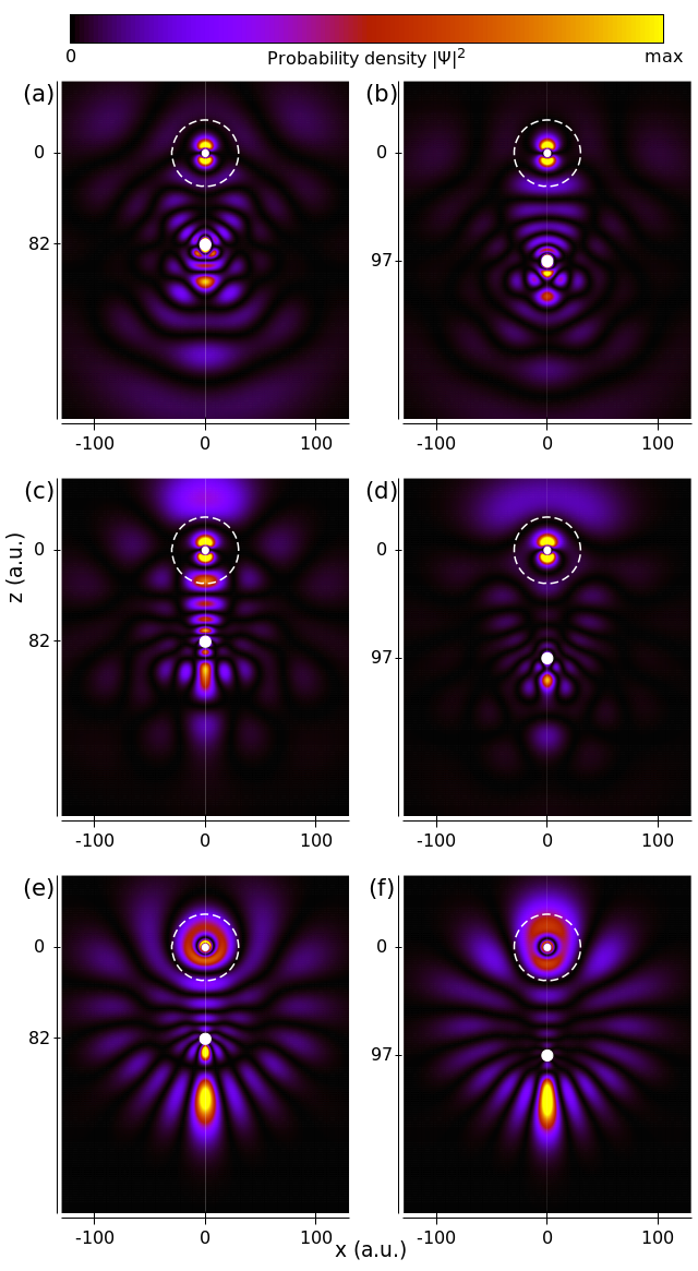
Figure 7: Two-dimensional maps of the Rydberg electron probability densities in the molecular states where the atomic states $12p$ and $10(l>3)$ are perturbed. The perturber is located in the center of the coordinate system and the white circle denotes the R-matrix sphere. The internuclear distances are marked on the vertical axes and corresponding points on the PECs are labeled in Fig. 4. The small vicinities of the atomic centers are discussed in Section III of Supplemental Material.

Below the avoided crossing with the PEC involving the Rb^- resonance ($R\lesssim 140$ a.u. in Fig. 4), none of the wave functions can be characterized as predominated by the $np$ states (see Fig. 7). All three of them have complicated structure with significant contributions of the higher angular momenta. Correspondingly, as it is illustrated in Fig. 4 for the state $12p$, the local minima and maxima of the oscillations in the PECs do not accurately correspond to the extremes and zeroes of the radial atomic Rydberg wave functions $np$.

The character of the PECs $\alpha$ and $\beta$ in Fig. 4 can be partially explained by the coupling of the degenerate hydrogen-like manifolds by the neutral perturber represented by the zero-range model. In that theory, the pseudopotential of the perturber in the partial waves $s$ [1] and $p$ [5, 16] yields in the basis of the degenerate atomic states two PECs that detach from the degenerate unperturbed asymptote. One of them descends with decreasing internuclear distance $R$ due to the e^--Rb resonance [37] and becomes oscillatory at smaller internuclear separations. This corresponds to the curve $\beta$ in Fig. 4. Hamilton et al. [5] associated it with the butterfly electronic states of the LRRM. However, the probability density maps of the Rydberg electron corresponding to the points of the PEC $\beta$ calculated in this work do not show the butterfly character [see Fig. 4 (c) and (d)].

In the energy range studied in this work, these oscillating PECs are intersected by the asymptotic energy $5s+np$. This suggests that this state $np$ is coupled to the nearest degenerate manifold above it and its perturbation by the neutral atom cannot be treated separately. As a result, there are no states in the studied region where the perturbation of the $np$ atomic Rydberg levels would be localized to the vicinity of the perturber [see Fig. 4 (a) and (b)]. This coupling is also the reason for the character of the Rydberg electron probability density different from the butterfly-like shape.

The authors in reference [5] studied higher excitations of the Rydberg atoms where the oscillatory segments of these deeply bound PECs are well separated from the other asymptotic thresholds. Therefore, the weakly locally perturbed Rydberg states $np$ exist and the perturbed high-$l$ states show the butterfly character.

The role of the coupling with the states $np$ was verified by performing a set of the test one-electron finite-range R-matrix calculations where the model potential of the perturber [20] was artificially made more attractive. The oscillatory structures in the obtained PEC $\beta$ descended towards lower energies while separating from the curve $\alpha$. The PEC $\alpha$ became consistent with other weakly perturbed non-degenerate states with the asymptotes $5s+n(l=0,2,3)$.

VI.2 Trilobite-like states

The other type of PEC detaching from the degenerate hydrogen-like manifolds at large values of $R$ in Figs. 1, 2 and 4, is monotonically increasing with the nuclei approaching each other (curve $\gamma$ in Fig. 4).

Figure 8: Detail of the PECs calculated using the finite-range one-electron model [20] (red dotted lines) near the asymptote $5s+9f$ and $5s+9(l>3)$ plotted along with the PECs obtained neglecting the e^--Rb interaction in the $p$-wave (blue crosses) (a). Mapping between the internuclear distance $R$ and the classical kinetic energy of the Rydberg electron $E_{k}$ at the location of the perturber (b) – aligned by the $R$-axis to panel (a). Dependence of the ${}^{3}S^{e}$ phase shift on $E_{k}$ [20] (c) – aligned by the axis $E_{k}$ to panel (b). The green dashed-dotted vertical guiding line denotes the point where $E_{k}=0$.

The Rydberg electron probability distributions [Fig. 7(e), (f)] along this curve show the dominating $s$-wave component in the vicinity of the perturber and the overall similarity to the trilobite states [1, 41].

Absence of the oscillatory structures in the PECs that support the bound vibrational states is a qualitative difference from the previously studied trilobite states at higher energies and larger $R$ (see [14] and references therein).

In the zero-range model, the oscillating segment of the trilobite PEC spans the interval of $R$ between two characteristic points. On the side of the large $R$, it is bounded by the classical turning point of the Rydberg electron beyond which the perturber interacts only with the non-oscillating exponentially decreasing region of the atomic Rydberg state. The left boundary of this segment is defined by the condition that the local kinetic energy of the Rydberg electron at the position of the perturber coincides with the Ramsauer minimum ($\approx 45$ meV) in the triplet $s$-wave e^--Rb phase shift. The repulsive character of the electron-atom interaction at smaller internuclear distances consequently yields repulsive PEC.

In order to elucidate the absence of the bound vibrational states associated with the trilobite electronic wave functions emerging from the calculations presented here, an artificial one-electron R-matrix calculation was performed where only the $s$-wave e^--Rb interaction was considered. The detail of the calculated PECs near the dissociation thresholds $5s+9f$ and $5s+9(l>3)$ is plotted in Fig. 8(a) by the blue crosses. This artificial trilobite-like PEC has a single shallow minimum below the dissociation threshold $5s+9(l>3)$ at $R\approx 148$ a.u. This suggests that in the range of energies and $R$ considered in this study, the attraction of the atoms due to the low-energy $s$-wave e^--Rb interaction is weak and it is compensated by the repulsive effect of the $p$-wave interaction included in the complete models.

The small extent of $R$ where the artificial trilobite-like PEC becomes attractive can also be qualitatively understood in terms of the zero-range model. The atomic Rydberg states that are subjects of this study are relatively compact. Therefore, a small increase of the distance from the positive core yields a rapid decrease of the local kinetic energy of the Rydberg electron [Fig. 8(b)]. As a result of this mapping, the e^--Rb interaction in the $s$-wave is attractive (and consequently induces attraction of the centers) in the narrow interval of distances from the positive core between the the point corresponding to the Ramsauer minimum at $127$ a.u. and the classical turning point at 162 a.u.

As can be seen in Fig. 8, the point where the artificial trilobite PEC changes its nature from the attractive to the repulsive (at $R\approx 135$ a.u.), does not accurately correspond to the Ramsauer minimum in the ${}^{3}S^{e}$ e^--Rb interaction. It is visible as the difference in $R$ and in $E_{k}$ marked by the magenta region. Since the difference of 8 a.u. is similar to the size of the ground-state Rb atom, this variation can be attributed to the effects of the atomic finite size. This is taken into account in the PECs calculated in this work while disregarded in the zero-range interpretation.

VII Conclusions

The two-electron R-matrix method [23] was applied to Rb₂ for a range of the internuclear separations between 37 a.u. and 200 a.u. in order to calculate the excited ${}^{3}\Sigma$ electronic states of this LRRM. In addition to the interaction between the Rydberg electron and the neutral perturber considered also in the zero-range models of the LRRMs, this approach also takes into account the effect of the Coulomb potential due to the positive Rydberg core on the valence electron of the perturber. The valence electron is explicitly represented and its interaction with the Rydberg electron is treated as true Coulomb repulsion.

The goal of the study presented in this article was to compare this advanced two-electron approach with the simple zero-range model at the intermediate internuclear separations $R<200$ a.u. where these can yield different energies. The PECs calculated using the two-electron R-matrix method showed similar overall character to those obtained from the zero-range model. The most notable differences appeared in the regions where the curves detach from the asymptotic energies of the degenerate hydrogen-like Rydberg states. Due to the low-energy e^--Rb resonance, significant probability density of the Rydberg electron is localized in the vicinity of the perturber. It is not surprising that these states are sensitive to the details of all the interactions involving the perturber.

The two-electron R-matrix technique also yields different energies than the one-electron methods in the classically forbidden regions of the Rydberg electron. These differences were attributed to the fact that the model e^--Rb interaction is in the one-particle models directly or indirectly parametrized by the kinetic energy of the Rydberg electron and their application in the classically forbidden region requires their extension towards the negative energies. These assumptions are not required in the two-electron R-matrix approach.

The zero-range model [1, 5] and the two-electron approach also yield different results at small internuclear separations among those studied in this work. This is due to the polarization of the perturber by the Coulomb tail of the potential due to the positive Rydberg atomic core. This effect can be in the one-electron models partially taken into account by including the polarization term $-\alpha_{d}/2R^{4}$ [33, 34, 35, 36].

The two-electron approach allowed for the calculation of the PECs associated with the excited state of the neutral perturber. The curves with the asymptotic energy of the state $5p+4d$ were presented in this article. The PECs can be well approximated by the atomic energy of the perturber in the state $5p$ weakly polarized by the distant Rydberg core. This character changes only at $R\lesssim 43$ a.u.

The wave functions of the Rydberg electron were calculated using the one-particle model based on the finite-range potential representation of the perturber [20].

The perturbation of the non-degenerate atomic Rydberg states $ns$, $nd$ and $nf$ (with respect to the positive Rydberg center) by neutral Rb atom yields the wave functions that retain their overall angular structure of the unperturbed atomic Rydberg states, the modification is localized in the vicinity of the perturber. On the other hand, the global character of the perturbed atomic Rydberg states $np$ changes rapidly even while the perturber is distant from the Rydberg core and the wave functions show very complicated nodal structure involving high angular momenta. This is due to the fact that in Rb₂, at the internuclear separations studied in this work, the energies of the long-range molecular butterfly-like states involving high angular momenta with respect to the positive core are very close to the energy levels of the atomic Rydberg states $np$.

Another category of the molecular states involving high angular momenta of the Rydberg electron, are the trilobite states. In the range of the internuclear separations studied here, the PECs associated with these states are anti-bonding (monotonically decreasing with the internuclear distance) and they do not possess any vibrationally bound states. This is due to very small interval of $R$ where the classical energy of the Rydberg electron allows it to interact attractively with the rubidium perturber in the $s$-wave. Moreover, the $s$-wave attraction is too weak and the overall nature is dictated by the repulsive $p$-wave.

*

Appendix A Unphysical steeply rising PECs

Figs. 1 and 5 show, among other, four very steeply rising PECs that do not appear in the results of the zero-range model. They are artifacts of the way in which the smooth matching of the inner-region and outer-region wave functions is performed on the R-matrix sphere. In the case when the matrix $\underline{\Gamma}$ in Eq. (14) becomes singular, an additional degree of freedom appears in the matching equations (9) and (12). The number of the matching conditions is not sufficient at those singular energies and the matching procedure yields an unphysical bound state.

For a fixed internuclear separation $R$, these artificial bound states appear at such energies $E_{x}$ where $\det\left[\underline{\Gamma}(E_{x})\right]=0$. Note, as can be seen from Eqs. (7) and (8), that $\underline{\Gamma}$ depends on the distance of the nuclei and on the radius $r_{0}$ and it does not depend on the interaction inside the R-matrix sphere. At each $E_{x}$, a vector $\mathbf{x}_{0}^{\prime}(r_{0})$ with the components $(x_{0}^{\prime})_{\overline{j}}(r_{0})$ exists on the sphere so that $\underline{\Gamma}(E_{x})\mathbf{x}_{0}^{\prime}(r_{0})=\mathbf{0}$. As a result, Eq. (9) yields at the energy $E_{x}$ for an arbitrarily selected outer-region solution $\mathbf{x}(r_{0})$ more general set of corresponding radial derivatives $\mathbf{x}^{\prime}(r_{0})$ than at other energies. Specifically, when $\mathbf{x}^{\prime}(r_{0})$ is a vector of the radial derivatives corresponding to the vector of the solutions $\mathbf{x}(r_{0})$ via Eq. (9), then $\mathbf{x}^{\prime}(r_{0})+\tau\mathbf{x}^{\prime}_{0}(r_{0})$ is also a vector of the radial derivatives corresponding to the same solution $\mathbf{x}(r_{0})$ for any real value of the scalar factor $\tau$.

Existence of at least a single value of $\tau$ for which Eqs. (12) and (13) are satisfied, in addition to Eq. (9), is a sufficient condition for a smooth matching of the outer-region solution to the inner-region wave function and, consequently, for an existence of the bound state at energy $E_{x}$. However, this is always possible, as the additional variable $\tau$ increases the total number of the variables in the homogeneous $N$-dimensional linear system formed by the Eqs. (12), (13) and (9) to $N+1$. This explains the fact, observed in the performed numerical calculations, that these steeply rising PECs do not depend on the interaction inside the R-matrix sphere.

Since these PECs are monotonic and they possess clear crossings with the other PECs, they can be easily distinguished from the physical PECs and they do not represent any complication for interpretation of the results. Another simple way of their identification is the identification of the energies and internuclear distances where the matrix $\underline{\Gamma}$ becomes singular.

These unphysical PECs descend in energy with increasing radius $r_{0}$. This is the reason for their absence in the PECs of H₂ presented in TC. Since the R-matrix sphere used there ($r_{0}=10$ a.u.) was significantly smaller than used in the results presented here, all the unphysical PECs were located above the studied energy interval.

References

- Greene et al. [2000] C. H. Greene, A. S. Dickinson, and H. R. Sadeghpour, Creation of Polar and Nonpolar Ultra-Long-Range Rydberg Molecules, Phys. Rev. Lett. 85, 2458 (2000).
- Bendkowsky et al. [2009] V. Bendkowsky, B. Butscher, J. Nipper, J. P. Shaffer, R. Löw, and T. Pfau, Observation of ultralong-range Rydberg molecules, Nature 458, 1005 (2009).
- Li et al. [2011] W. Li, T. Pohl, J. M. Rost, S. T. Rittenhouse, H. R. Sadeghpour, J. Nipper, B. Butscher, J. B. Balewski, V. Bendkowsky, R. Löw, and T. Pfau, A homonuclear molecule with a permanent electric dipole moment, Science 334, 1110 (2011).
- Booth et al. [2015] D. Booth, S. T. Rittenhouse, J. Yang, H. R. Sadeghpour, and J. P. Shaffer, Production of trilobite Rydberg molecule dimers with kilo-Debye permanent electric dipole moments, Science 348, 99 (2015).
- Hamilton et al. [2002] E. L. Hamilton, C. H. Greene, and H. R. Sadeghpour, Shape-resonance-induced long-range molecular Rydberg states, J. Phys. B 35, L199 (2002).
- Niederprüm et al. [2016] T. Niederprüm, O. Thomas, T. Eichert, C. Lippe, J. Pérez-Ríos, C. H. Greene, and H. Ott, Observation of pendular butterfly Rydberg molecules, Nat. Commun. 7, 12820 (2016).
- DeSalvo et al. [2015] B. J. DeSalvo, J. A. Aman, F. B. Dunning, T. C. Killian, H. R. Sadeghpour, S. Yoshida, and J. Burgdörfer, Ultra-long-range Rydberg molecules in a divalent atomic system, Phys. Rev. A 92, 031403(R) (2015).
- Ding et al. [2019] R. Ding, S. K. Kanungo, J. D. Whalen, T. C. Killian, F. B. Dunning, S. Yoshida, and J. Burgdörfer, Creation of vibrationally-excited ultralong-range Rydberg molecules in polarized and unpolarized cold gases of 87Sr, J. Phys. B: At., Mol. Opt. Phys. 53, 014002 (2019).
- Schmid et al. [2018] T. Schmid, C. Veit, N. Zuber, R. Löw, T. Pfau, M. Tarana, and M. Tomza, Rydberg Molecules for Ion-Atom Scattering in the Ultracold Regime, Phys. Rev. Lett. 120, 153401 (2018).
- Engel et al. [2019] F. Engel, T. Dieterle, F. Hummel, C. Fey, P. Schmelcher, R. Löw, T. Pfau, and F. Meinert, Precision spectroscopy of negative-ion resonances in ultralong-range rydberg molecules, Phys. Rev. Lett. 123, 073003 (2019).
- Deiß et al. [2020] M. Deiß, S. Haze, J. Wolf, L. Wang, F. Meinert, C. Fey, F. Hummel, P. Schmelcher, and J. Hecker Denschlag, Observation of spin-orbit-dependent electron scattering using long-range Rydberg molecules, Phys. Rev. Research 2, 013047 (2020).
- Fey et al. [2020] C. Fey, F. Hummel, and P. Schmelcher, Ultralong-range Rydberg molecules, Mol. Phys. 118, e1679401 (2020).
- Shaffer et al. [2018] J. P. Shaffer, S. T. Rittenhouse, and H. R. Sadeghpour, Ultracold Rydberg molecules, Nat. Commun. 9, 1965 (2018).
- Eiles [2019] M. T. Eiles, Trilobites, butterflies, and other exotic specimens of long-range Rydberg molecules, J. Phys. B: At., Mol. Opt. Phys. 52, 113001 (2019).
- Blatt and Weisskopf [2012] J. Blatt and V. Weisskopf, Theoretical nuclear physics (Dover Publications, 2012) pp. 73–77.
- Omont [1977] A. Omont, On the theory of collisions of atoms in Rydberg states with neutral particles, J. Phys. (Paris) 38, 1343 (1977).
- Anderson et al. [2014] D. A. Anderson, S. A. Miller, and G. Raithel, Angular-momentum couplings in long-range Rydberg molecules, Phys. Rev. A 90, 062518 (2014).
- Eiles and Greene [2017] M. T. Eiles and C. H. Greene, Hamiltonian for the inclusion of spin effects in long-range Rydberg molecules, Phys. Rev. A 95, 042515 (2017).
- Fey et al. [2015] C. Fey, M. Kurz, P. Schmelcher, S. T. Rittenhouse, and H. R. Sadeghpour, A comparative analysis of binding in ultralong-range Rydberg molecules, New J. Phys. 17, 055010 (2015).
- Khuskivadze et al. [2002] A. A. Khuskivadze, M. I. Chibisov, and I. I. Fabrikant, Adiabatic energy levels and electric dipole moments of Rydberg states of and dimers, Phys. Rev. A 66, 042709 (2002).
- Bellos et al. [2013] M. A. Bellos, R. Carollo, J. Banerjee, E. E. Eyler, P. L. Gould, and W. C. Stwalley, Excitation of Weakly Bound Molecules to Trilobitelike Rydberg States, Phys. Rev. Lett. 111, 053001 (2013).
- Carollo et al. [2017] R. A. Carollo, J. L. Carini, E. E. Eyler, P. L. Gould, and W. C. Stwalley, High-resolution spectroscopy of Rydberg molecular states of near the asymptote, Phys. Rev. A 95, 042516 (2017).
- Tarana and Čurík [2016] M. Tarana and R. Čurík, Adiabatic potential-energy curves of long-range Rydberg molecules: Two-electron -matrix approach, Phys. Rev. A 93, 012515 (2016).
- Hostler and Pratt [1963] L. Hostler and R. H. Pratt, Coulomb Green’s Function in Closed Form, Phys. Rev. Lett. 10, 469 (1963).
- Davydkin et al. [1971] V. Davydkin, B. Zon, N. Manakov, and L. Rapoport, Quadratic Stark effect on atoms, Sov. Phys. JETP 33, 70 (1971).
- Aymar et al. [1996] M. Aymar, C. H. Greene, and E. Luc-Koenig, Multichannel rydberg spectroscopy of complex atoms, Rev. Mod. Phys. 68, 1015 (1996).
- Robicheaux [1991] F. Robicheaux, Driving nuclei with resonant electrons: Ab initio study of , Phys. Rev. A 43, 5946 (1991).
- Tennyson [2010] J. Tennyson, Electron–molecule collision calculations using the r-matrix method, Phys. Rep. 491, 29 (2010).
- Eiles [2018] M. T. Eiles, Formation of long-range Rydberg molecules in two-component ultracold gases, Phys. Rev. A 98, 042706 (2018).
- Tarana and Čurík [2019] M. Tarana and R. Čurík, -matrix calculations of electron collisions with a lithium atom at low energies, Phys. Rev. A 99, 012708 (2019).
- Bahrim et al. [2002] C. Bahrim, U. Thumm, A. A. Khuskivadze, and I. I. Fabrikant, Near-threshold photodetachment of heavy alkali-metal anions, Phys. Rev. A 66, 052712 (2002).
- Lorenzen and Niemax [1983] C.-J. Lorenzen and K. Niemax, Quantum Defects of the Levels in I and I, Phys. Scr. 27, 300 (1983).
- Schlagmüller et al. [2016a] M. Schlagmüller, T. C. Liebisch, H. Nguyen, G. Lochead, F. Engel, F. Böttcher, K. M. Westphal, K. S. Kleinbach, R. Löw, S. Hofferberth, T. Pfau, J. Pérez-Ríos, and C. H. Greene, Probing an Electron Scattering Resonance using Rydberg Molecules within a Dense and Ultracold Gas, Phys. Rev. Lett. 116, 053001 (2016a).
- Schlagmüller et al. [2016b] M. Schlagmüller, T. C. Liebisch, F. Engel, K. S. Kleinbach, F. Böttcher, U. Hermann, K. M. Westphal, A. Gaj, R. Löw, S. Hofferberth, T. Pfau, J. Pérez-Ríos, and C. H. Greene, Ultracold Chemical Reactions of a Single Rydberg Atom in a Dense Gas, Phys. Rev. X 6, 031020 (2016b).
- Liebisch et al. [2016] T. C. Liebisch, M. Schlagmüller, F. Engel, H. Nguyen, J. Balewski, G. Lochead, F. Böttcher, K. M. Westphal, K. S. Kleinbach, T. Schmid, A. Gaj, R. Löw, S. Hofferberth, T. Pfau, J. Pérez-Ríos, and C. H. Greene, Controlling Rydberg atom excitations in dense background gases, J. Phys. B: At., Mol. Opt. Phys. 49, 182001 (2016).
- Whalen et al. [2017] J. D. Whalen, F. Camargo, R. Ding, T. C. Killian, F. B. Dunning, J. Pérez-Ríos, S. Yoshida, and J. Burgdörfer, Lifetimes of ultralong-range strontium Rydberg molecules in a dense Bose-Einstein condensate, Phys. Rev. A 96, 042702 (2017).
- Bahrim and Thumm [2000] C. Bahrim and U. Thumm, Low-lying and states of , and , Phys. Rev. A 61, 022722 (2000).
- Bahrim et al. [2001] C. Bahrim, U. Thumm, and I. I. Fabrikant, Negative-ion resonances in cross sections for slow-electron–heavy-alkali-metal-atom scattering, Phys. Rev. A 63, 042710 (2001).
- Stanojevic and Côté [2020] J. Stanojevic and R. Côté, Rydberg electron-atom scattering in forbidden regions of negative kinetic energy, J. Phys. B: At., Mol. Opt. Phys. 53, 114002 (2020).
- Safronova and Safronova [2011] M. S. Safronova and U. I. Safronova, Critically evaluated theoretical energies, lifetimes, hyperfine constants, and multipole polarizabilities in , Phys. Rev. A 83, 052508 (2011).
- Granger et al. [2001] B. E. Granger, E. L. Hamilton, and C. H. Greene, Quantum and semiclassical analysis of long-range Rydberg molecules, Phys. Rev. A 64, 042508 (2001).