Short time dynamics of tracer in ideal gas

Abstract

A small tagged particle immersed in a fluid exhibits the Brownian motion and diffuses at the long-time scale. Meanwhile, at the short-time scale, the dynamics of the tagged particle cannot be simply described by the usual generalized Langevin equation with the Gaussian noise, since the number of collisions between the tagged particle and fluid particles is rather small. At such a time scale, we should explicitly consider individual collision events between the tagged particle and the surrounding fluid particles. In this study, we analyzed the short-time dynamics of the tagged particle in an ideal gas, where we do not have static nor hydrodynamic correlations between fluid particles. We performed event-driven hard sphere simulations and show that the short-time dynamics of the tagged particle is correlated even under such an idealized situation. Namely, the velocity autocorrelation function becomes negative when the tagged particle is relatively light and the fluid density is relatively high. This result can be attributed to the dynamical correlation between collision events. To investigate the physical mechanism, which causes the dynamical correlation, we analyzed the correlation between successive collision events. We found that the tagged particle can collide with the same ideal gas particle several times, and such collisions cause the strong dynamical correlation for the velocity.

I introduction

A particle immersed in a fluid exhibits a random motion, which is widely known as the Brownian motionBrown (1828). The Brownian motion originates from the interaction between the tagged particle (tracer) and the particles which compose the surrounding fluid (fluid particles). In principle, the dynamics of the tracer is deterministic because the full system, which consists of the tracer and the fluid particles, obeys the Hamiltonian dynamics. However, if we observe only the tracer, the dynamics looks stochastic (at least apparently).

For the description of such stochastic dynamics of the tracer, the generalized Langevin equation (GLE)van Kampen (2007); Sekimoto (2010) has been employed in many cases. The GLE is a stochastic differential equation, which incorporates the memory effect (memory kernel) and the random noise. The properties of the memory kernel and the random noise reflects the statistical properties of the surrounding fluid. Formally, the projection operator methodKawasaki (1973) gives the expression for the memory kernel and the noise is related to the memory kernel via the fluctuation-dissipation relation. The dynamic equation for the tracer is given as

$$M\frac{d^{2}\bm{r}(t)}{dt^{2}}=-\int_{-\infty}^{t}dt^{\prime}\,K(t-t^{\prime})\frac{d\bm{r}(t^{\prime})}{dt^{\prime}}+\bm{\xi}(t),$$ (1)

where $\bm{r}$ and $M$ are the position and mass of the tracer, $K(t)$ is the memory kernel, and $\bm{\xi}(t)$ is the random noise. The random noise satisfies

$$\langle\bm{\xi}(t)\rangle=0,\qquad\langle\bm{\xi}(t)\bm{\xi}(t^{\prime})\rangle=k_{B}TK(|t-t^{\prime}|)\bm{1},$$ (2)

where $\langle\dots\rangle$ represents the statistical average, $k_{B}$ is the Boltzmann constant, $T$ is the temperature, and $\bm{1}$ is the unit tensor.

The projection operator formalism does not tell us the full properties of the noise $\bm{\xi}(t)$. It gives only the first and second moments as eq (2). Therefore, in many practical cases, the noise is assumed to be Gaussian. Then the dynamic equation for the tracer is fully specified and can be analytically solvedFox (1977). Such type of a GLE with the Gaussian noise is utilized to analyze various experimental dataMason and Weitz (1995); Mason et al. (1997); Li et al. (2010); Kheifets et al. (2014); Huang et al. (2011). The diffusion of the tracer can be also directly studied by molecular dynamics simulations. Recently, the memory kernels for some systems are precisely calculated from the molecular dynamics simulationsLesnicki et al. (2016); Straube et al. (2020). For example, the power-law type long-time tail, which originates from hydrodynamic modes, is reported for a Lennard-Jones fluidLesnicki et al. (2016). It should be noted that, in most cases, a tracer is assumed to be large and massivePatravic (2008). However, in some cases, a tracer could be rather small and light. For example, if we interpret a molecule which is dissolved into a fluid as a tracer, the tracer size is comparable to the fluid particles and the mass of the tracer is also comparable to that of a fluid particle. (For example, if we consider a mixture system which consists of isotopes and interpret a light species as a tracer, the tracer mass can be slightly smaller (or larger) than unityKiriushcheva and Kuzmin (2005).) The dynamics of a tracer particle can be experimentally measured by such as the scattering, and we need to describe the dynamics of the tracer particle to analyze the experimental data.

Here we emphasize that the Gaussian noise approximation is not justified a priori. Naively, we expect that the approximation is reasonable because the noise would be Gaussian as a results of the accumulated many forces due to the collisions of surrounding fluid particles. As far as the number of collisions is sufficiently large, the average force will converge to a Gaussian noise by the central limit theorem. Conversely, when the number of collisions is not enough, the Gaussian noise approximation does not work properly. Such a situation can be realized when we consider the dynamics of a single tagged particle in a dilute gas. The Gaussianity of the noise can be evaluated via the Gaussianity of the displacement, since the displacement is a linear combination of the noise (by eq (1)). For instance, Yamaguchi and KimuraYamaguchi and Kimura (2001) investigated the dynamics of a single hard-sphere in a dilute hard-sphere gas. They reported that the distribution function for the displacement is non-Gaussian at a short time scale. We should be careful when we employ the Gaussian noise approximation.

The tracer dynamics at the short time scale in a dilute fluid can be described, for example, by the gas kinetic theoryChapman and Cowling (1990). To illustrate the dynamics with a small number of collisions, we should consider the individual collision events explicitly. Then, we expect that the dynamics would be modeled by the sequence of the collision events. Burshtein and KrongauzBurshtein and Krongauz (1995) modeled the dynamics of a tracer in a hard-sphere fluid as a sequence of the collision events. They assumed simple statistics for the collision events (the statistical distributions of the waiting time between successive collisions and the velocity change distribution are decoupled, and given as simple hypothetical forms) and calculated the dynamical quantities such as the velocity autocorrelation function (VAC). Their model can successfully reproduce some dynamical properties. However, we note that the employed statistics would be a matter of further discussion. We expect that the statistics depends on the fluid density rather strongly. When the fluid is dilute, then the collisions are statistically almost independentChapman and Cowling (1990). Some assumptions in the Burshtein-Krongauz model will be justified in such a case. However, when the fluid is rather dense, the situation becomes very complex. In a dense hard-sphere fluidAlder and Wainwright (1970); Herman and Alder (1972), the statistics of collisions would depend on various factors. For example, it can be related to the structure of the fluid. Recently, Mizuta et alMizuta et al. (2019) performed a series of molecular dynamics simulations for a fullerene particle immersed in a liquid Argon. They reported that the dynamics of fullerene particles is affected both by the hydrodynamics and structure of the fluid. Although their result is interesting, it seems difficult to quantitatively separate the contributions of individual factors.

The statistics of collision events can also depend on the mass of the tracer. For a collision between two hard spheres, velocities of spheres after the collision depend on the velocities before the collision and masses of two hard spheres. The collision statistics depends on the cross-section of the collision and the relative velocity. For the collision between a tracer particle and a fluid particle, the statistics of the relative velocity depends on the masses of the tracer and the fluid particle. Also, the momentum exchange between the tracer and the ideal gas particle depends on the mass ratio. Then, if the mass of the tracer is changed, the collision statistics would be changed (by the change of the relative velocity distribution). If the tracer mass is sufficiently larger than the fluid molecule mass, the momentum of the tracer will not be largely affected by a single collision. However, if the tracer mass is relatively small, the momentum largely changes even by a single collision, and consequently the back reflection and the negative velocity autocorrelation of the tracer can occurAlder et al. (1974); Herman and Alder (1972). The statistics of the collision events would not be simple in this case. Such collision statistics can be naturally handled by utilizing the methods developped in the gas kinetic theoryChapman and Cowling (1990); Eder (1977), instead of the GLE. We can describe the dynamics by the Boltzmann equation or by the Fokker-Planck equation, and then employ some collision statistics to calculate the dynamical quantities such as the velocity autocorrelation. For dilute gases, we may reasonably assume that collisions are statistically independent. Then the collision distribution can be described by the Poisson process, some dynamical quantities behave qualitatively different from the GLE with the Gaussian noise approximation. For example, the mass dependence of the diffusion coefficient can be explained by the gas kinetic theory. If the gas density is relatively high, however, the description by the gas kinetic theory becomes nontrivial. The Burshtein-Krongauz model would be interpreted as a phenomenological extension of the kinetic theory to a relatively dense system. The extension of the GLE by combining non-Gaussian type processes which mimic collisions has also been proposedGelin (2014); Gelin et al. (2015). However, the microscopic origin of the negative velocity correlation has not been fully clarified yet.

In this paper, we investigated the dynamics of the tracer particle at the short-time scale, from the view point of collision events. As we mentioned, the statistics of collision events and the short-time dynamics of the tracer depend both on the fluid density and the tracer mass. They are also affected by several different factors such as the fluid structure and the hydrodynamic interaction. To eliminate such factors other than the fluid density and the tracer mass, we consider systems where fluid particles do not interact with each other (the ideal gas). We investigated the dynamics of the tracer in the ideal gas by the hard-sphere simulations. We performed series of simulations with various parameter sets. We found that the tracer exhibits a rather complex dynamics at the short-time scale, even by such an idealized and simplified model. We analyzed the dynamics of the tracer on the basis of the collision type dynamics by Burshtein and KrongauzBurshtein and Krongauz (1995). Below, We will show that the correlation between sequential collisions is important to describe the short-time dynamics of the tracer.

II Model and Method

We consider the dynamics of a tracer immersed in an ideal gas by a numerical simulation. In this work, we use the term “an ideal gas” as a gas composed of point masses, which do not interact with each other at all. The point masses do not exchange their momenta via collisions. The tracer collides with the ideal gas particles whereas the ideal gas particles do not collide each other. We modeled the tracer as a hard sphere particle, and employed the standard hard sphere simulation methodAlder and Wainwright (1959). Both the tracer and ideal gas particles move ballistically until they collide. The velocity of the tracer and ideal gas particles are instantaneously changed when they collide.

We consider a single tracer particle and $N$ ideal gas particles in the cubic simulation box with the periodic boundary conditions. We set the number of ideal gas particles as $N=10^{5}$ for all the simulations. We express the masses of the tracer and ideal gas particles as $M$ and $m$, the size of the tracer as $\sigma$ (the size of the ideal gas particles is $0$), the temperature of the system as $T$, and the number density of the ideal gas particles as $\rho$. (Here, the particle density is related to the system volume $\mathcal{V}$ as $\rho=N/(\mathcal{V}-\pi\sigma^{3}/6)$.) We employ dimensionless units where the unit energy, unit mass, and unit length are $k_{B}T$ ($k_{B}$ is the Boltzmann constant), $m$ and $\sigma$, respectively. In the dimensionless units, the system can be characterized only by two parameters: $M$ and $\rho$. We varied the density $\rho$ in the range from $10^{-2}$ to $10^{3}$, and the mass $M$ in the range from $10^{-2}$ to $10^{3}$.

The initial state of the simulation was generated as follows. The tracer particle was located at the box center, and the ideal gas particles were dispersed randomly in the box. (The position of a newly generated ideal gas particle should not overlap to the tracer.) The initial velocities of the tracer and ideal gas particles were sampled from the Maxwell-Boltzmann distribution. To prevent the center of mass of the system from drifting, we subtracted the velocity of the center of mass from all the particles in the system. Then, the velocities of particles were rescaled to reduce the average kinetic energy to $3/2$. Since the momentum is conserved in the hard sphere simulation, the center of mass does not move during a simulation. After the initial state was generated, we evolved the system by using the established procedure for the hard-sphere simulationAlder and Wainwright (1959).

Although the hard-sphere simulation itself is rather simple and clear, we should be careful about the handling of the images due to the periodic boundary condition. In this simulation, the mean free path of the tracer is long and this leads to unexpected overlaps between the tracer and images of ideal gas particles. To avoid such overlaps, we performed simulations as follows.

1. Generate the initial state.

2. Find the ideal gas particle(the target particle), which collides the tracer judging from their positions and velocities. Let the waiting time for the collision of this particle is $\Delta t_{1}$.

3. Find the ideal gas particle, which has the maximum relative velocity to the tracer along the axis of the simulation box. From the maximum relative velocity $V_{\text{max}}$, obtain the minimum time of collision of the image particle to the tracer as $\Delta t_{2}=(L-\sigma)/(2V_{\text{max}})$, where $L(=\mathcal{V}^{1/3})$ is the box length.

4. If $\Delta t_{2}<\Delta t_{1}$, update the position of all particles by the step size $\Delta t_{2}$, then proceed to $t\to t+\Delta t_{2}$ and repeat the update unless $\Delta t_{1}\leq\Delta t_{2}$. When $\Delta t_{1}\leq\Delta t_{2}$ is satisfied, update the position of all particles by the step size $\Delta t_{1}$, then proceed to $t\to t+\Delta t_{1}$ to attain the collision.

5. Update the velocity of the tracer and the target particle according to the collision.

6. Repeat from step2 to step5 until 10 million collisions.

From the trajectories of the tracer, we calculated several dynamical quantities: We calculate the mean-square displacement (MSD), the non-Gaussian parameter (NGP)Rahman (1964), and the velocity autocorrelation function (VAC) defined as

$$g(t)\equiv\langle\Delta\bm{r}^{2}(t)\rangle,$$ (3)

$$\alpha(t)\equiv\frac{3\langle\Delta\bm{r}^{4}(t)\rangle}{5\langle\Delta\bm{r}^{2}(t)\rangle^{2}}-1,$$ (4)

$$C(t)\equiv\frac{\langle\bm{V}(t)\cdot\bm{V}(0)\rangle}{\langle\bm{V}^{2}\rangle}.$$ (5)

Here, $\Delta\bm{r}(t)\equiv\bm{r}(t)-\bm{r}(0)$ is the displacement of the tracer , and $\bm{V}(t)$ is the velocity of the tracer. $\langle\dots\rangle$ represents the statistical average. We also calculated a few quantities which characterize the change of the tracer velocity by collisions. They will be introduced later.

Before we show the simulation results, here we briefly comment on the effect of the system size to the simulation results. In our model, the ideal gas particles can change their velocities only via the collision to the tracer. Thus the relaxation time for the velocity of an ideal gas particle becomes very long and it depends on the system size. One may consider that the velocity distribution of the ideal gas particles deviate from the equilibrium distribution. Also, one may suspect that the dynamics of the tracer strongly depends on the system size. As far as we examined, fortunately, the velocities of the ideal gas particles obey the equilibrium Maxwell-Boltzmann distribution. Some dynamical quantities of the tracer, such as the MSD and VAC, do not show measurable system size dependence (unless the system size is too small and comparable to the tracer size). Therefore, we conclude that the system size dependence for simulation results can be safely neglected (at least for the analyses shown below).

III Results

Figure 1(a) shows the mass dependence of the MSD for the ideal gas density of $\rho=1$. In a short-time region, the ballistic behavior $\langle\Delta\bm{r}^{2}(t)\rangle\propto t^{2}$ is observed, and the MSD decreases as $M$ increases. This behavior is consistent with the fact that the average absolute value of velocity decreases as $M$ increases. In a long-time region, diffusive behavior $\langle\Delta\bm{r}^{2}(t)\rangle\propto t$ is observed, and the MSD decreases as $M$ increases. This result means that the diffusion coefficient of tracer depends on $M$. One may argue that the $M$-dependence is counter-intuitive because the GLE (1) predicts that the inertia term does not contribute to the long-time dynamics. However, from the view point of the gas kinetic theory, the diffusion coefficient can depend on the massChapman and Cowling (1990). A similar behavior has been reported for the motion of a tracer in Lennard-Jones fluidsBearman and Jolly (1981); Nuevo et al. (1995) and hard-sphere fluidsAlder et al. (1974). Nevertheless, in this work, we do not discuss the $M$-dependence of the diffusion coefficient.

Figure 1(b) shows the $M$ dependence of the NGP. The parameters are the same as Figure 1(a). The NGP increases with time in the ballistic regime, exhibits a peak in the transitional regime, and decays in the diffusive regime. The peak increases as $M$ decreases. This result means that the statistics of the displacement is non-Gaussian except in the diffusive regime when $M$ is small. The non-Gaussian behavior is observed in various systems and often attributed to the heterogeneity of the environment. For example, the glass forming liquidsKob et al. (1997) and polymer solutionsXue et al. (2016) work as heterogeneous environments for a tracer. However, in our system, the ideal gas particles never have the structures and thus the non-Gaussian behavior cannot be attributed to the heterogeneity of the environment. Therefore, we consider that non-Gaussian behavior has the kinetic origin. In our system, the tracer dynamics is affected only by the collisions and the non-Gaussian behavior can be attributed to the properties of collisions. (Yamaguchi and and Kimura also reported similar non-Gaussian behavior for a dilute hard sphere fluidYamaguchi and Kimura (2001).)

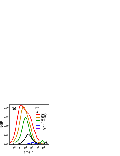
Figure 1: (a) MSD and (b) NGP of a tracer in the ideal gas for various $M$. The density of the ideal gas is $\rho=1$.

Figures 2 shows the $\rho$-dependence of MSD and NGP with a constant mass of the tracer ($M=1$). We observe the MSD collapses into a single curve in the ballistic region. The MSD deviates from the ballistic behavior to the diffusive behavior, and the crossover time decreases as $\rho$ increases. This $\rho$-dependence is due to the change of the mean free path. As seen in Fig 1, we observe the non-negligible peak for the NGP. The peak value of the NGP is almost constant for $\rho\leq 1$, whereas the value slightly increases as $\rho$ increases for $\rho\geq 1$. Although such increase of NGP against $\rho$ is commonly observed for liquids with heterogeneous structuresvan Swol and Petsev (2014), we have no heterogeneity in our model, as mentioned above.

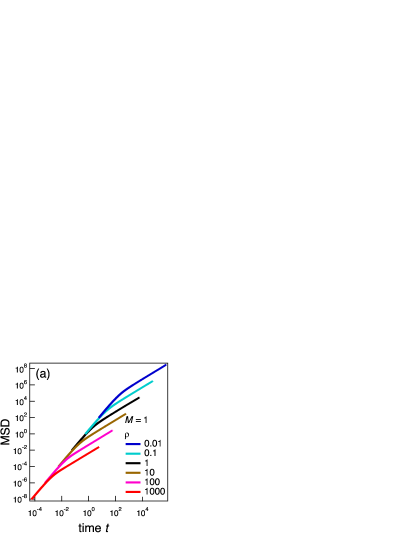
Figure 2: (a) MSD and (b) NGP of a tracer in the ideal gas for various $\rho$. The mass of the tracer is $M=1$.

From the mass and density dependence shown above, we conclude that the dynamics of the tracer qualitatively depends on the mass and the density. If the mass is large ($M\gtrsim 1$), the dynamics of the particle can be reasonably described as the Gaussian process. (The GLE with the Gaussian noise approximation is reasonable.) If the density is low ($\rho\lesssim 1$), the dynamics of the tracer can be expressed by the ballistic motion and collisions (as the standard gas kinetic theoryChapman and Cowling (1990)). However, if the mass is small and the density is high ($M\lesssim 1$ and $\rho\gtrsim 1$), the dynamics seems not to be expressed as a simple and intuitive model. We consider that this is caused by the “dynamic” correlation. (In our system, the fluid has no static structure since it is an ideal gas.) Our result suggests that, the dynamic correlation solely gives such an apparently counter-intuitive behavior. A simple interpretation is that something like a “cage” would be dynamically formed and the tracer effectively feels confinement at the short-time scale. However, this behavior is not trivial, and to investigate it in detail, we performed some additional simulations for several parameter sets for $M\lesssim 1$ and $\rho\gtrsim 1$.

Figure 3 shows the MSD and NGP for several different parameter sets. From Figure 3(a), we find that the MSD shows unexpected behavior for $M=0.01$ and $\rho=100$. Namely, the MSD does not show the plain crossover from the ballistic to diffusion behavior, and we observe an intermediate subdiffusive region between the ballistic and diffusive regions. The similar behavior of the MSD has been reported for some systems such as glass forming liquids and polymer solutionsGe et al. (2018); Vyas et al. (2016). Although the data are not explicitly presented, similar behavior has been also reported for the multi particle collision dynamics (MPCD) type modelMalevanets and Kapral (2000). In Figure 3(b), we observe a strong peak of NGP for $M=0.01$ and $\rho=100$. (Intuitively, the peak time for the NGP ($t_{\text{peak}}$) corresponds to the relaxation time of the tracer velocity. This interpretation seems to be consistent with the MSD data. The MSD exhibits the ballistic behavior for $t\lesssim t_{\text{peak}}$, and the diffusive behavior for $t\gtrsim t_{\text{peak}}$.) Thus demonstrated, we confirm that our system exhibits nontrivial dynamical behavior for small $M$ and high $\rho$. These results seem not to be simply described by the GLE or the gas kinetic theory. Some questions naturally arises. What is the origin of such nontrivial behavior? How can we describe the dynamics?

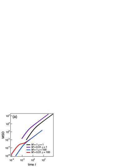
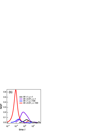
Figure 3: (a)MSD and (b)NGP of a tracer for several sets of the mass $M$ and the ideal gas density $\rho$.

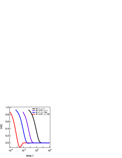
Figure 4: VAC of a tracer for several sets of the mass and the ideal gas density. The parameters are the same as in Figure 3.

Here we recall that our simulation model is a collision-driven hard-sphere molecular dynamics model. In our model, the tracer moves ballistically and the velocity changes only by the collisions with the ideal gas particles. Therefore, it would be reasonable for us to concentrate on the velocity of the tracer. Figure 4 shows the VAC of a tracer particle for the same parameter sets as Figures 3. For the case of $M=0.01$ and $\rho=100$, the VAC becomes negative at the intermediate time region. The negative correlation in the VAC means that the tracer is effectively reflected back by collisions (the back reflection). A negative VAC is usually attributed to the strong static and dynamic correlations between fluid particles. However, in our system, the ideal gas particles do not have static and dynamic correlations and thus we cannot attribute the negative VAC to the correlations between fluid particles. A possible intuitive interpretation is as follows. If the mass of the tracer is small, the tracer has a large velocity compared with the surrounding ideal gas particles. Also, due to the large mass contrast, the momentum of an ideal gas particle is almost not affected when the tracer and the ideal gas particle collides. Thus, we may interpret the ideal gas particles as almost fixed obstacles. Under such a situation, the back reflection behavior may occur. Meanwhile, we should notice that the effect of the back reflection becomes especially strong when the density is high. To clarify the short-time dynamics, therefore, we should analyze the collisions in detail. In addition to the short-time dynamics, the long-time dynamics is important for some analyses. The VAC typically exhibits so-called the long-time tail at the long time region. In our simulation results, however, the power-law type long-time tail is not clearly observed, at least in the examined time scale. (We may observe the long-time tail at the very long time scale, but it is beyond the scope of this work and thus we do not consider the long time region in what follows.)

Burshtein and KrongauzBurshtein and Krongauz (1995) considered a similar negative velocity correlation in hard sphere fluids. They analyzed the dynamics of a hard sphere carefully and proposed a simple model which describes the motion of a hard sphere. They modeled a process as a sequence of collision events, which we may interpret as a renewal process. They assumed that the time interval between two successive collisions is sampled from a waiting time distribution $P(\tau)$, and there is no correlation between successive waiting times. They also assumed that the velocity of the hard sphere is stochastically changed from $\bm{V}$ to $\bm{V}^{\prime}$, and the new velocity $\bm{V}^{\prime}$ is sampled from the velocity distribution $P(\bm{V}^{\prime}|\bm{V})$. Their model claims that the negative velocity correlation can emerge if both of the following two conditions are satisfied; (a) the waiting time distribution $P(\tau)$ is not a exponential distribution, and (b) the average velocity after a collision is negatively correlated to the velocity before the collision, $\langle\bm{V}^{\prime}\cdot\bm{V}\rangle<0$. Although their model seems plausible, some assumptions in their model cannot be fully justified. Thus we investigate the statistics of collisions in our simulations below.

Figure 5 shows the waiting time distribution between two successive collision events. In this work, we define the waiting time as the time interval between two successive collision events. (We do not distinguish whether the tracer collides to the same ideal gas particle or not.) The waiting time $\tau$ is normalized by the average waiting time $\bar{\tau}\equiv\int d\tau\,\tau P(\tau)$. We observe that the distribution function for the normalized waiting time is almost independent of $M$ and $\rho$. Moreover, the waiting time distribution can be reasonably fit to the exponential distribution. Naively, the exponential waiting time distribution means that the collision events are statistically independent. Thus this result implies that the Poisson distribution for the number of collisions during a finite time period. However, this naive argument is physically not fully justified. This is because the statistics of the waiting time generally depends on the tracer velocity. The observed waiting time distribution should be interpreted as the average waiting time distribution over the tracer velocity. This average waiting time distribution seems to be well described by the exponential distribution. (We show the calculations for the waiting time distributions in Appendix A.) Anyway, the assumption (a) is not satisfied. According to the Burshtein-Krongauz model, if the waiting time distribution is exponential, then the VAC is always positive. Clearly, this is not consistent with our simulation result in Figure 4. We expect that some assumptions by Burshtein and Krongauz would not be valid (at least for our system). We will discuss the statistical properties of collisions in detail, in the next section.

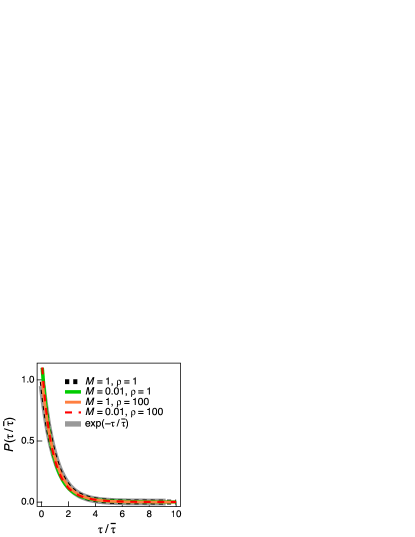
Figure 5: The waiting time distribution function $P(\tau)$ with different values of the mass $M$ and the ideal gas density $\rho$. The waiting time $\tau$ is normalized by the average $\bar{\tau}$ as $\tau/\bar{\tau}$. For comparison, the exponential distribution $P(\tau)=(1/\bar{\tau})\exp(-\tau/\bar{\tau})$ is also plotted.

IV Discussions

IV.1 Gaussianity

In this subsection, we discuss the Gaussianity of the dynamics of the tracer. Our simulation results (Figures 1-3) show that the tracer exhibits the non-Gaussian behavior even if the surrounding fluid is an ideal gas. The NGP strongly depends on the tracer mass $M$, and if $M$ is sufficiently large, the NGP becomes small. Therefore, if $M$ is sufficiently large, the dynamics of the tracer can be reasonably described by a Gaussian process. For such a case, the GLE with the Gaussian noise can be utilized.

As we mentioned, the GLE with the Gaussian noise has been widely employed to analyze experimental data. But our results imply that the application of the GLE may not be fully justified in some cases. Here we discuss validity of the GLE for some experimental systems. Recent progress of experimental techniques enabled us to experimentally measure the short-time ballistic motion of a tracer particleLi et al. (2010); Huang et al. (2011). Li et alLi et al. (2010) investigated the dynamics of $3\text{{\textmu}m}$ beads in dilute gases ($2.75\rm{kPa}$ and $99.8\rm{kPa}$) at the micro second scale. The mass of the tracer is about $10^{-10}\text{g}$, whereas the mass of the gas molecule is about $10^{-23}\text{g}$. Clearly the mass ratio is very large (about $10^{13}$) and thus we expect that the tracer dynamics is reasonably described by the GLE. Note that the memory effect is negligible in this system and thus the GLE reduces to a simple Langevin equation. Huang et alHuang et al. (2011) measured the dynamics of a tracer in a fluid. Although the fluid density is much larger than the experiments by Li et al, the mass ratio is estimated to be the same order as that of Li et al. Therefore, we conclude that for typical experimental conditions for the short-time dynamics of a tracer particle, the GLE (or the Langevin equation) with the Gaussian noise can be safely employed.

However, the argument above does not fully justify the use of the Langevin equation to analyze the other experimental data. The Langevin equation is utilized for various analyses of experimental data, even at the very small objects. Some examples are the light absorbance in the infrared (IR) spectroscopy and the diffusion in the nuclear magnetic resonance (NMR). In the IR spectroscopy, the absorbance is often calculated based on the oscillator model for polar functional groups. A functional group is not sufficiently small compared with the surrounding objects, and the analyses based on the Langevin equation may not be justified. Actually, Roy et alRoy et al. (2011) measured two dimensional correlation spectra and reported that the dynamics is not Gaussian. In the NMR, the diffusion of a proton (or other atom) is estimated from the NMR signal based on a simple diffusion equation by the Brownian motion. (Even if the Langevin equation is not formally justified, we empirically know the analyses based on the simple Langevin equation gives reasonable results in most cases.) We consider that if the conventional analyses do not give physically reasonable result, we should analyze the data carefully based on the collision dynamics. (Strictly speaking, we should employ quantum dynamics to analyze the IR or NMR dataTanimura (2006). However, the naive incorporation of the Gaussian noise like a Langevin thermostat to quantum systems is questionableVan Kampen (2005). Some ideas in this work might be useful to consider the modeling of thermostats.)

IV.2 Correlation between Collisions

In this subsection, we consider the collision events in detail. As we showed, the waiting time distribution $P(\tau)$ in our system is well described by the exponential distribution. (The assumption (a) in the Burshtein-Krongauz model is not satisfied.) The Burshtein-Krongauz model does not give a negative VAC for the exponential waiting time distribution. Here, it should be mentioned that the exponential waiting time distribution is also reported for hard sphere fluidsTalbot (1992). The reason why the waiting time obeys the exponential distribution is not clear. Because our system is similar to hard sphere systems in some aspects, we expect there is a common mechanism which gives the exponential waiting time distribution.

In the Burshtein-Krongauz model, the correlation between the velocities before and after the collision is also an important quantity. To investigate the statistical properties of the collision events in detail, we consider the correlation between velocities by introducing the quantity defined as $\gamma_{1}=\langle\bm{V}^{\prime}\cdot\bm{V}\rangle_{\text{coll}}/\langle\bm{V}^{2}\rangle_{\text{coll}}$ (where $\bm{V}$ and $\bm{V}^{\prime}$ are the velocities of the tracer before and after a collision event and $\langle\cdots\rangle_{\text{coll}}$ represents the statistical average with respect to collisions). If we assume that the distribution of the velocity after the collision is Gaussian, a collision event statistics can be characterized only by this $\gamma_{1}$. In the Burshtein-Krongauz model, $\gamma_{1}$ should be negative to give a negative VAC.

It would be informative to analyze $\gamma_{1}$. In our system, the statistics of the fluid particles is simple and thus we can theoretically calculate $\gamma_{1}$, which can be expressed in a simple form as

$$\gamma_{1}=\frac{3M}{3M+4}.$$ (6)

See Appendix B for the details of the model and calculations. Here, we should note that $\gamma_{1}$ given by eq (6) is independent of the ideal gas density $\rho$. Therefore, we expect that $\gamma_{1}>0$ holds for any $M$ and $\rho$. We show the prediction by eq (6) together with the simulation data in Figure 6. We find that eq (6) reasonably reproduces the simulation result without any fitting parameters. From these results, we conclude that the velocity correlation factor $\gamma_{1}$ cannot be negative in our model. This means that the assumption (b) in the Burshtein-Krongauz model is not satisfied, neither. From these results, both two assumptions in the Burshtein-Krongauz model are not satisfied in our system. However, the original idea of the Burshtein-Krongauz model that the dynamics of the tracer is described by the successive collision events seems to be reasonable. We expect that with several modifications, the Burshtein-Krongauz type model may explain the dynamical behavior. Before we consider the modification, we should investigate the detailed statistical properties of the collision events.

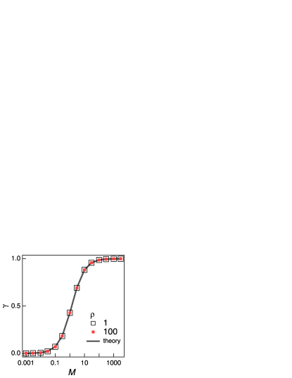
Figure 6: The correlation factor of the velocity before and after a collision, $\gamma_{1}$. The mass $M$ dependence of $\gamma_{1}$ with two different values of $\rho$ is shown. The data for different $\rho$ are almost the same and data points look fully overlapped.

We consider that the successive collisions can be correlated in our system. Then the correlation factor $\gamma_{1}$ is not sufficient to characterize the properties of the collision events. We should investigate multiple collisions which can be correlated. We define the correlation factor for the multiple collision events as

$$\gamma_{n}\equiv\frac{\langle\bm{V}_{i+n}\cdot\bm{V}_{i}\rangle_{\text{coll}}}{\langle\bm{V}_{i}^{2}\rangle_{\text{coll}}}.$$ (7)

If the successive collision events are independent, we have $\gamma_{n}=\gamma_{1}^{n}$. If the successive collision events are not statistically independent, $\gamma_{n}$ may behave in a different way. Figure 7 shows the correlation factor $\gamma_{n}$ directly calculated from the simulations. For $M=1$ and $\rho=1$, $\gamma_{n}$ decays exponentially as $n$ increases, which seems to be consistent with the estimate based on the statistically independent collisions. For $M=0.01$ and $\rho=100$, however, we find that $\gamma_{n}$ does not exhibit the exponential decay. Clearly, $\gamma_{n}$ has a negative peak at $n=3$, while $\gamma_{1}$ and $\gamma_{2}$ are almost zero. Therefore, the successive collision events are not statistically independent if the mass is small and the ideal gas density is high. As a consequence, we cannot simply apply the Burshtein-Krongauz model.

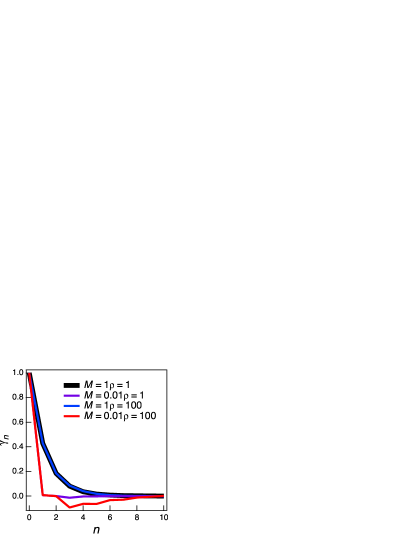
Figure 7: The correlation factor of the velocity for multiple collisions, $\gamma_{n}$. $n$ represents the number of collisions. The data for different values of the mass $M$ and the ideal gas density $\rho$ are shown.

Based on this result, here we attempt to construct the modified version of the Burshtein-Krongauz model. From the simulation results of the correlation factor data for the multiple collisions $\gamma_{n}$, it would be possible to treat several collision events (for example, $n=3$ or $4$ events) as a coarse-grained event. Then we can express the correlation factor for the coarse-grained collision event as $\gamma_{\text{eff}}=\gamma_{n}$. Also, the waiting time distribution between two coarse-grained events becomes

$$\begin{split}P_{\text{eff}}(\tau)&=\int d\tau_{1}\dots d\tau_{n}\,\delta(\tau-\tau_{1}-\dots\tau_{n})P(\tau_{1})\dots P(\tau_{n})\\ &=\frac{t^{n-1}}{(n-1)!\tau^{n}}\exp(-\tau/\bar{\tau}).\end{split}$$ (8)

Eq (8) is the gamma distribution, and is clearly different from the exponential distribution, for $n\geq 2$. If we assume that coarse-grained collision events are statistically independent, we can utilize the Burshtein-Krongauz model by interpreting their collision events as the coarse-grained collision events. With such a coarse-graining, the negative velocity correlation can be reasonably explained by the (modified) Burshtein-Krongauz model.

IV.3 Origin of Negative Correlation

Although the Burshtein-Krongauz model seems to work with some modifications, it does not explain why the correlation factor $\gamma_{n}$ becomes negative for $n=3$. To clarify the emergence mechanism of the negative correlation, we analyze the correlation factor in further detail. Because now we know that the successive collisions are not independent, it would be reasonable to consider whether the correlation comes from the same ideal gas particle or not. It would be informative to decompose the correlation factor $\gamma_{n}$ into the correlation by the collisions to the same ideal gas particle and the collisions to different ideal gas particles. We thus define the self and distinct parts of the correlation factor for multiple collisions:

$$\gamma_{n} =\gamma_{n}^{(s)}+\gamma_{n}^{(d)},$$ (9)

$$\gamma_{n}^{(s)} \equiv\frac{\langle\bm{V}_{i+n}\bm{V}_{i}\,I(K_{i+1}=K_{i+n})\rangle}{\langle\bm{V}_{i}^{2}\rangle},$$ (10)

$$\gamma_{n}^{(d)} \equiv\frac{\langle\bm{V}_{i+n}\bm{V}_{i}\,I(K_{i+1}\neq K_{i+n})\rangle}{\langle\bm{V}_{i}^{2}\rangle},$$ (11)

where $I(\dots)$ takes $1$ if the argument is true and takes $0$ if not, and $K_{i}$ represents the index of the ideal gas particle which collides to the tracer at the $i$-th collision event. Figure 8 shows the self and distinct parts of the collision factor, for $M=0.01$ and $\rho=100$. From Figure 8, we find that $\gamma_{n}^{(s)}$ is negative for $n\geq 3$ whereas $\gamma_{n}^{(d)}$ is positive for all $n$. This result means that the collisions by different particles do not contribute to the negative correlation, and the negative correlation emerges from the collisions with the same particle.

The reason why the correlation occurs at $n=3$ can be now understood rather intuitively. We consider the sequence of several collision events. At the first collision ($n=1$), the correlation is always positive ($\gamma_{1}>0$), as we demonstrated. By this first collision, the tracer and the ideal gas particle exchange the momentum and they move apart from each other. Therefore at the second collision ($n=2$) the tracer cannot collide to the same ideal gas particle as the first collision. After the second collision, the momentum of the tracer is changed again, and the tracer can move towards the ideal gas particle which collided at the first collision. Thus, for $n\geq 3$, we have the correlation with the same ideal gas particle.

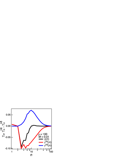
Figure 8: The self and distinct part of the correlation factor for multiple collisions, $\gamma_{n}^{(s)}$ and $\gamma_{n}^{(d)}$. The mass and the ideal gas densities are $M=0.01$ and $\rho=100$. The full correlation factor is given as $\gamma_{n}=\gamma_{n}^{(s)}+\gamma_{n}^{(d)}$.

Before we end this subsection, we briefly mention about the MSD. As known well, the MSD and the VAC can be related via the Kubo formulaKubo (1966). The MSD is obtained by doubly integrating the VAC. Conversely, we have the velocity correlation as

$$\frac{d^{2}\langle{\Delta\bm{r}}^{2}(t)\rangle}{dt^{2}}=\langle{\bm{V}}(t)\cdot{\bm{V}}(0)\rangle.$$ (12)

If the velocity correlation becomes negative, at a certain time we should have $\langle\bm{V}(t)\cdot\bm{V}(0)\rangle=0$. This fact means that if we have the negative velocity correlation, we may observe an inflection point in the MSD. In addition, if the negative correlation is strong, the MSD may exhibit an intermediate region between the short-time ballistic and the long-time diffusive regions. Indeed, we observed such nontrivial intermediate region in Figure 3(a). Interestingly, the time scale where we observe this intermediate region seems to be the same where we observe the strong peak of the NGP in Figure 3(b). Therefore, we consider that the collision with the same ideal gas particle is the origin of various nontrivial short-time behavior of the tracer.

IV.4 Comparison with Other Simulations

In this subsection, we compare our results with the other simulations. Mizuta et alMizuta et al. (2019) investigated the dynamics of the single fullerene in the liquid Argon by using the molecular dynamics simulation. They investigated the dynamics of the fullerenes at various time scales. At the short time scale where the time is shorter than the Enskog time, they showed that the Enskog theoryChapman and Cowling (1990) reasonably describes the VAC of a fullerene. The Enskog theory is based on the gas kinetic theory, and thus the results by Mizuta et al implies that the short-time scale dynamics is governed by collisions. The Enskog time is the time scale where approximately only one collision per fluid particle occurs. At the longer time scales, the behavior deviates from the Enskog theory. Mizuta et al reported the effect of the fullerene size. For the small fullerene (or for a fluid particle), they reported that the VAC becomes negative at the short-time scale region. This result is qualitatively consistent with ours. However, we should stress that fluid particles strongly interact with each other in their system. Therefore, we cannot quantitatively compare our result with their simulation data. We expect that our analyses would be useful to study some aspects of the short-time scale dynamics in realistic systems like those investigated by Mizuta et al.

At the long-time scale where the time is longer than the kinematic time of the momentum diffusion over the particle size, they reported that the GLE works reasonably. Intuitively, at the long-time scale, the fluid can be treated as a continuum fluid rather than discrete particles. Then the GLE can be safely employed. This intuitive expectation consistent with their result. Conversely, our system does not have the interactions between the fluid particles, and thus it seems not reasonable to treat fluid particles as a continuum fluid. In our system, the fluid particles move ballistically until they collide with the tracer. Because we employed the periodic boundary condition, the mean free path $\lambda$ of the ideal gas particles depends on the system size as $\lambda\approx{\mathcal{V}}/{\sigma^{2}}$. The Knudsen number Kn can be estimated as follows:

$$\mathrm{Kn}=\frac{\lambda}{\sigma}=\frac{\mathcal{V}}{\sigma^{3}}.$$ (13)

Clearly, the obtained $\mathrm{Kn}$ is much larger than $1$ for sufficiently a large system ($\mathrm{Kn}\gg 1$). Therefore, we conclude that the ideal gas can not be regarded as a continuum fluid for the tracer. Consequently, our system does not obey usual continuum hydrodynamic equations such as the Navier-Stokes equation. Our system is designed to study the short-time dynamics and should not be used to study the long-time dynamics. This would explain why we do not observe the long-time tail in the long time region. To apply the continuum hydrodynamic equations to our model, we should consider very long time scale and very large length scale. The long-time tail may be observed at such a very long time scale, although it would be longer than the current simulation time scale. Because the fluid cannot be expressed by usual continuum hydrodynamic equations, it would not be straightforward to interpret the non-Markovian memory effect in our system. (Normally, the memory kernel can be related to the molecular scale hydrodynamicsLesnicki et al. (2016); Straube et al. (2020); Mizuta et al. (2019).) As far as the author knows, it is not clear whether the collision-based description can be successfully related to the hydrodynamic description or not. It would be an interesting future work to study how the collision-based and hydrodynamic descriptions are connected.

We also compare our results with the simulation by Alder and AlleyAlder et al. (1974). They investigated the effect of the tracer mass and the tracer size on the dynamics in a hard sphere fluid. They analyzed the VAC of the tracer and showed that the VAC of the tracer has the negative peak when the mass of the tracer is small. This result is consistent with our result. According to our analyses, such a negative VAC can be attributed to the property of the multiple (typically three) sequential collisions. Although the VAC data by Alder and Alley are not analyzed in terms of collisions, their data seems to be consistent with our analyses: the VAC becomes negative at the time where three collisions occur on average. This implies that our theory holds, at least qualitatively, even under the existence of the hard sphere interaction between fluid particles. We expect that the interpretations and analyses based on the collision events are useful to study the short-time dynamics of various systems.

V Conclusions

We investigated the short-time dynamics of the tracer in the ideal gas. Our system can be characterized only by two parameters, the mass of the tracer $M$ and the fluid density $\rho$, in the dimensionless units. We performed hard-sphere type simulations and calculated various dynamical quantities such as the MSD, NGP, and VAC, for various values of $M$ and $\rho$. The dynamical behavior is largely affected by $M$ and $\rho$. For $M\gtrsim 1$, the NGP is very small and the GLE with the Gaussian noise can describe the dynamics well. For $M\lesssim 1$, however, the dynamics cannot be described by a Gaussian stochastic process. We should explicitly consider collision events to describe the dynamics for $M\lesssim 1$. For $\rho\lesssim 1$, the behavior is relatively simple and seems to be consistent with the standard gas kinetic theory. Meanwhile, for $M\lesssim 1$ and $\rho\gtrsim 1$, some nontrivial dynamical properties have been observed. For example, the VAC exhibits a negative value.

To study the origin of such non-trivial behavior, we analyzed the collision events in detail. We showed that the waiting time distribution between two successive collisions is almost the exponential distribution, and the correlation factor $\gamma_{1}$ is almost positive. The Burshtein-Krongauz model predicts that the VAC is always positive for our system, but it is not consistent with the simulation result. We introduced the correlation factor between multiple collisions, $\gamma_{n}$, to further investigate the statistical properties of collision events. We showed that the velocities before and after multiple collisions are rather strongly correlated, and this correlation is the origin of the negative VAC. In addition, we showed that the strong correlation mainly comes from the multiple collisions between the tracer and the same ideal gas particle.

Although our system is highly idealized and simplified, we believe that our results are informative to analyze realistic systems. The dynamical correlation between multiple collision events would exist in realistic systems. The analyses based on the collision picture, such as the analysis of the correlation factor $\gamma_{n}$ and the decomposition of it to $\gamma_{n}^{(s)}$ and $\gamma_{n}^{(d)}$ would be useful to analyze the short-time dynamics in various systems. The analyses for the systems with interactions such as the hard sphere fluid and the Lennard-Jones fluid would be an interesting future work.

Appendix A Waiting Time Distribution

In this appendix, we roughly estimate the waiting time distirbution for the tracer particle in an ideal gas. The collision statistics depends on the relative velocity of the tracer to an ideal gas particle. The distribution of the relative velocity is generally not that simple (as we consider in Appendix B). However, under some special conditions, the distribution reduces to rather simple forms. If the tracer mass is sufficiently large ($M\gg 1$), the tracer velocity becomes very small compared with the surrounding ideal gas particles. The relative velocity distribution approximately coincides to the Maxwell-Boltzmann distribution of the ideal gas particle. Then, the collision statistics do not depend on the tracer velocity $\bm{V}$. Individual collision events are expected to be statistically independent, and then the number of collisions during a finite time period should obey the Poisson distribution. This Poission distribution can be directly related to the exponential waiting time distribution. Therefore, we expect that the waiting time distribution becomes exponential if $M$ is sufficiently large.

On the other hand, if the tracer mass is sufficiently small ($M\ll 1$), the relative velocity distribution is almost the same as the tracer velocity $\bm{V}$. Here we consider the case where the tracer velocity $\bm{V}$ is fixed to be constant. In this case, the relative velocity distribution is also fixed and we will observe several collision events during a finite time period. The individual collision events are statistically independent, and thus we expect the exponential waiting time distribution. Therefore, we have

$$P(\tau|\bm{V})=\frac{1}{\bar{\tau}(\bm{V})}\exp(-\tau/\bar{\tau}(\bm{V})),$$ (14)

where $\bar{\tau}(\bm{V})$ is the average waiting time for the tracer velocity $\bm{V}$. We expect that the interval between collisions decreases as the tracer velocity increases. Naively, we consider the average waiting time can be related to the tracer velocity as $\bar{\tau}(\bm{V})=\Lambda/|\bm{V}|$ where $\Lambda$ is a mean free path, and we assume $\Lambda$ is independent of $\bm{V}$. (The mean free path $\Lambda$ depends on the ideal gas density $\rho$.) Then we can express the waiting time distribution as

$$P(\tau)=\int d\bm{V}P(\tau|\bm{V})P_{\text{eq}}(\bm{V})=\int_{0}^{\infty}dV\,\frac{V}{\Lambda}\exp(-\tau V/\Lambda)P_{\text{eq}}(V),$$ (15)

where $V\equiv|\bm{V}|$, and $P_{\text{eq}}(\bm{V})$ and $P_{\text{eq}}(V)$ represent the equilibrium distribution functions for $\bm{V}$ and $V$, respectively. The waiting time distribution can be then calculated to be

$$\begin{split}P(\tau)&=\int_{0}^{\infty}dV\,\frac{4\pi V^{3}}{\Lambda}\left(\frac{M}{2\pi}\right)^{3/2}\exp\left(-\frac{\tau V}{\Lambda}-\frac{MV^{2}}{2}\right)\\ &=\frac{1}{\Lambda\sqrt{M}}\left[-(3+\tilde{\tau}^{2})\tilde{\tau}\exp\left(\frac{\tilde{\tau}^{2}}{2}\right)\mathrm{erfc}\left(\frac{\tilde{\tau}}{\sqrt{2}}\right)+\sqrt{\frac{2}{\pi}}(2+\tilde{\tau}^{2})\right],\end{split}$$ (16)

with $\tilde{\tau}\equiv\tau/\Lambda\sqrt{M}$. Eq (16) can be reasonably approximated by the exponential distribution:

$$P(\tau)\approx\frac{1}{\Lambda\sqrt{M}}\sqrt{\frac{8}{\pi}}\exp\left(-\sqrt{\frac{8}{\pi}}\frac{\tau}{\Lambda\sqrt{M}}\right).$$ (17)

Thus if $M$ is sufficiently small, the waiting time distribution approximately reduces to the exponential distribution with the average waiting time $\bar{\tau}\approx\Lambda\sqrt{\pi M/8}$.

From the estimates shown above, both for sufficiently large and sufficiently small $M$ cases, we have the exponential distributions. At the intermediate $M$ cases, we intuitively expect that the waiting time distribution would be expressed in a similar expression to eq (16). We replace $V$ by the relative velocity $v^{\prime}=|\bm{V}-\bm{v}|$ ($\bm{v}$ is the velocity of an ideal gas particle):

$$P(\tau)=\int_{0}^{\infty}dv^{\prime}\,\frac{v^{\prime}}{\Lambda}\exp(-\tau v^{\prime}/\Lambda)P_{\text{eq}}(v^{\prime}),$$ (18)

where $P_{\text{eq}}(v^{\prime})$ is the equilibrium relative velocity distribution. The relative velocity obeys the Maxwell-Boltzmann distribution and thus we approximately have the exponential waiting time distribution (as the case of the sufficiently small $M$ case). Therefore the waiting time distribution will be well approximated by the exponential distribution for any $M$. This is consistent with the simulation results shown in Figure 5.

Appendix B Calculation of $\gamma_{1}$

In this appendix, we show the detailed calculation of the correlation factor $\gamma_{1}$. We consider the equilibrium system, in which the ideal gas particles are distributed uniformly in space, and the velocity is sampled from the Maxwell-Boltzmann distribution.

In what follows, we calculate $\gamma_{1}$ in the dimensional units (not in the dimensionless units in the main text) for the sake of clarity. We describe the velocities before and after the collision as $\bm{V}$ and $\bm{V}^{\prime}$. We describe the velocity of the ideal gas particle which collides to the tracer as $\bm{v}$. We calculate $\gamma_{1}=\langle\bm{V}^{\prime}\cdot\bm{V}\rangle_{\text{coll}}/\langle\bm{V}^{2}\rangle_{\text{coll}}$ under the following assumptions:

1. The ideal gas particles are uniformly distributed in space.

2. Both the tracer and ideal gas particles obey the Maxwell-Boltzmann distribution:

   $$P_{t}(\bm{V}) =\left(\frac{M}{2\pi k_{B}T}\right)^{3/2}\exp\left(-\frac{M\bm{V}^{2}}{2k_{B}T}\right),$$ (19)

   $$P_{g}(\bm{v}) =\left(\frac{m}{2\pi k_{B}T}\right)^{3/2}\exp\left(-\frac{m\bm{v}^{2}}{2k_{B}T}\right).$$ (20)

We consider the velocity of the tracer after the collision with an ideal gas particle. The velocity after the collision $\bm{V}^{\prime}$ is simply obtained from the momentum and the energy conservation:

$$\bm{V}^{\prime}=\bm{V}+\frac{2m}{M+m}\hat{\bm{r}}\cdot(\bm{v}-\bm{V})\hat{\bm{r}},$$ (21)

where $\hat{\bm{r}}$ is the unit vector between the tracer and the ideal gas particle when the collision occurs (the direction vector). To calculate $\gamma_{1}$, we need to calculate the ensemble average. We can express the average of the internal product of velocities $\langle\bm{V}^{\prime}\cdot\bm{V}\rangle_{\text{coll}}$ as

$$\langle\bm{V}^{\prime}\cdot\bm{V}\rangle_{\text{coll}}=\frac{\int d\bm{V}d\bm{v}d\hat{\bm{r}}\,P_{t}(\bm{V})P_{g}(\bm{v})P_{d}(\hat{\bm{r}})|\bm{v}-\bm{V}|\,\bm{V}^{\prime}\cdot\bm{V}}{\int d\bm{V}d\bm{v}d\hat{\bm{r}}\,P_{t}(\bm{V})P_{g}(\bm{v})P_{d}(\hat{\bm{r}})|\bm{v}-\bm{V}|},$$ (22)

where $P_{d}(\hat{\bm{r}})$ represents the equilibrium distribution of the direction vector. The factor $|\bm{v}-\bm{V}|$ comes from the fact that the collision frequency is proportional to the relative velocity between the tracer and the ideal gas particle. (The average with respect to collision $\langle\dots\rangle_{\text{coll}}$ is different from the simple equilibrium average by this factor.) From eqs (21) and (22),

$$\gamma_{1}=1+\frac{2m}{M+m}\frac{\int d\bm{V}d\bm{v}d\hat{\bm{r}}\,P_{t}(\bm{V})P_{g}(\bm{v})P_{d}(\hat{\bm{r}})\left|\bm{v}-\bm{V}\right|\,\hat{\bm{r}}\cdot(\bm{v}-\bm{V})\hat{\bm{r}}\cdot\bm{V}}{\int d\bm{V}d\bm{v}d\hat{\bm{r}}\,P_{t}(\bm{V})P_{g}(\bm{v})P_{d}(\hat{\bm{r}})\left|\bm{v}-\bm{V}\right|\bm{V}^{2}}.$$ (23)

We can rewrite eq (23) in a simpler form by introducing the reduced mass and the relative velocity. We define $\nu=M+m$, $\mu=Mm/\nu$, $\bm{u}=(M\bm{V}+m\bm{v})/\nu$, $\bm{v}^{\prime}=\bm{v}-\bm{V}$. Then eq (23) reduces to

$$\gamma_{1}=1+\frac{2m}{M+m}\frac{\displaystyle\int d\bm{u}d\bm{v}^{\prime}d\hat{\bm{r}}\,P_{d}(\hat{\bm{r}})|\bm{v}^{\prime}|(\hat{\bm{r}}\cdot\bm{v}^{\prime})\,\hat{\bm{r}}\cdot\left(\bm{u}-\frac{m}{\nu}\bm{v}^{\prime}\right)\exp\left(-\frac{\nu\bm{u}^{2}+\mu\bm{v}^{\prime 2}}{2k_{B}T}\right)}{\displaystyle\int d\bm{u}d\bm{v}^{\prime}d\hat{\bm{r}}\,P_{d}(\hat{\bm{r}})|\bm{v}^{\prime}|\left(\bm{u}-\frac{m}{\nu}\bm{v}^{\prime}\right)^{2}\exp\left(-\frac{\nu\bm{u}^{2}+\mu\bm{v}^{\prime 2}}{2k_{B}T}\right)}$$ (24)

We calculate the integral in the denominator of the second term in the right hand side of eq (24). The integrand does not depend on $\hat{\bm{r}}$ and thus we can easily perform the integral over $\hat{\bm{r}}$. Then we have

$$\begin{split}&\int d\bm{u}d\bm{v}^{\prime}d\hat{\bm{r}}\,P_{d}(\hat{\bm{r}})|\bm{v}^{\prime}|\left(\bm{u}-\frac{m}{\nu}\bm{v}^{\prime}\right)^{2}\exp\left(-\frac{\nu\bm{u}^{2}+\mu\bm{v}^{\prime 2}}{2k_{B}T}\right)\\ &=\int d\bm{u}d\bm{v}^{\prime}|\bm{v}^{\prime}|\left(\bm{u}-\frac{m}{\nu}\bm{v}^{\prime}\right)^{2}\exp\left(-\frac{\nu\bm{u}^{2}+\mu\bm{v}^{\prime 2}}{2k_{B}T}\right)\\ &=\pi^{3/2}\left(2k_{B}T\right)^{9/2}\left(\frac{3}{\nu^{5/2}\mu^{2}}+\frac{4m^{2}}{\nu^{7/2}\mu^{3}}\right).\end{split}$$ (25)

Next we calculate the integral in the numerator of the second term in the right hand side of eq (24). Without loss of generality, we can set the direction of the relative velocity parallel to the $z$-axis: $\bm{v}^{\prime}=[0,0,v^{\prime}]$. For convenience, we rewrite the direction vector in the spherical coordinate, as $\hat{\bm{r}}=[\sin\theta\cos\phi,\sin\theta\sin\phi,\cos\theta]$. To proceed the calculation, we need the distribution function for the direction vector. Now a collision occurs between the tracer particle fixed at the origin and the ideal gas particles which moves parallel to the $z$-axis, with the velocity $v^{\prime}$. Then the distribution of the normal vector should be proportional to the direction vector which is projected onto the $xy$ plane:

$$P_{d}(\bm{\hat{r}}_{n})\propto|\sin\theta\cos\theta|.$$ (26)

In addition, not all the ideal gas particles can collide to the tracer. For $v^{\prime}>0$, the probability distribution becomes

$$P_{d}(\theta,\phi)=\begin{cases}-{\sin\theta\cos\theta}/{\pi}&(\pi/2\leq\theta\leq\pi),\\ 0&(\text{otherwise}).\end{cases}$$ (27)

Similarly, for $v^{\prime}<0$, we have

$$P_{d}(\theta,\phi)=\begin{cases}{\sin\theta\cos\theta}/{\pi}&(0\leq\theta\leq\pi/2),\\ 0&(\text{otherwise}).\end{cases}$$ (28)

By utilizing eqs (27) and (28), finally we have

$$\begin{split}&\int d\bm{u}d\bm{v}^{\prime}d\hat{\bm{r}}\,P_{d}(\hat{\bm{r}})|\bm{v}^{\prime}|(\hat{\bm{r}}\cdot\bm{v}^{\prime})\,\hat{\bm{r}}\cdot\left(\bm{u}-\frac{m}{\nu}\bm{v}^{\prime}\right)\exp\left(-\frac{\nu\bm{u}^{2}+\mu\bm{v}^{\prime 2}}{2k_{B}T}\right)\\ &=-2\pi^{3/2}\left(2k_{B}T\right)^{9/2}\frac{m}{\nu^{5/2}\mu^{3}}.\end{split}$$ (29)

By substituting eqs (25) and (29) into eq (24), we have the following simple expression for $\gamma_{1}$:

$$\gamma_{1}=\frac{3M}{3M+4m}.$$ (30)

This gives eq (6) in the main text. From this derivation, it would be rather trivial that $\gamma_{1}$ does not have the negative value.

References

- Brown (1828) R. Brown, Phil. Mag. 4, 161 (1828).
- van Kampen (2007) N. G. van Kampen, Stochastic Processes in Physics and Chemistry, 3rd ed. (Elsevier, Amsterdam, 2007).
- Sekimoto (2010) K. Sekimoto, Stochastic Energetics, Lect. Notes Phys., Vol. 799 (Springer, Berlin, 2010).
- Kawasaki (1973) K. Kawasaki, J. Phys. A: Math. Nucl. Gen. 6, 1289 (1973).
- Fox (1977) R. F. Fox, J. Math. Phys. 18, 2331 (1977).
- Mason and Weitz (1995) T. G. Mason and D. A. Weitz, Phys. Rev. Lett. 74, 1250 (1995).
- Mason et al. (1997) T. G. Mason, K. Ganesan, J. H. vanZanten, D. Wirtz, and S. C. Kuo, Phys. Rev. Lett. 79, 3282 (1997).
- Li et al. (2010) T. Li, S. Kheifets, D. Medellin, and M. G. Raizen, Science 328, 1673 (2010).
- Kheifets et al. (2014) S. Kheifets, A. Simha, K. Melin, T. Li, and M. G. Raizen, Science 343, 1493 (2014).
- Huang et al. (2011) R. Huang, C. Isaac, K. M. Taute, , B. Lukić, S. Jeney, M. G. Raizen, and E.-L. Florin, Nat. Phys. 7, 576 (2011).
- Lesnicki et al. (2016) D. Lesnicki, R. Vuilleumier, A. Carof, and B. Rotenberg, Phys. Rev. Lett. 116, 147804 (2016).
- Straube et al. (2020) A. V. Straube, B. G. Kowalik, R. R. Netz, and F. Höfling, Com. Phys. 3, 126 (2020).
- Patravic (2008) J. Patravic, J. Chem. Phys. 129, 114502 (2008).
- Kiriushcheva and Kuzmin (2005) N. Kiriushcheva and S. Kuzmin, Physica A: Statistical Mechanics and its Applications 352, 509 (2005).
- Yamaguchi and Kimura (2001) T. Yamaguchi and Y. Kimura, J. Chem. Phys. 114, 3029 (2001).
- Chapman and Cowling (1990) S. Chapman and Cowling, The mathematical theory of non-uniform gases: an account of the kinetic theory of viscosity, thermal conduction and diffusion in gases, 3rd ed. (Cambridge University Press, 1990).