Critical Limits in a Bump Attractor Network of Spiking Neurons

Abstract.

A bump attractor network is a model that implements a competitive neuronal process emerging from a spike pattern related to an input source. Since the bump network could behave in many ways, this paper explores some critical limits of the parameter space using various positive and negative weights and an increasing size of the input spike sources The neuromorphic simulation of the bump-attractor network shows that it exhibits a stationary, a splitting and a divergent spike pattern, in relation to different sets of weights and input windows. The balance between the values of positive and negative weights is important in determining the splitting or diverging behaviour of the spike train pattern and in defining the minimal firing conditions.

1. Introduction

The bump attractor network is a biologically inspired network able to describe several functions of the brain. Formally, it is a set of recurrently connected nodes (neurons) that have a stable pattern due to their time dynamics. The bump attractor is a particular case of an attractor network (Eliasmith:2007, ) in which the behaviour is stationary instead of cyclic or chaotic. This is why it is also called a stationary bump.

In computational neuroscience, there are also several types of attractor neural networks that are linked with specific brain functions, e.g., memorization, action planning, recognition and classification. The use of the attractor network framework permits the application of theories and methodologies of dynamical systems that can investigate their characteristics (e.g., stability vs. instability, convergence vs. divergence, stationary vs. non-stationary, etc.).

The brain processes multi-modal information coming from different sources of inputs. Although there are several modalities of stimuli (within the subject himself such as thinking and recalling, reasoning, or from outside of the body as the general perception of the sensory inputs), the brain selects and analyses this huge amount of information, that is often ambiguous, fragmented, and noisy. Therefore, the brain should make a decision and capture information that is relevant and use it to make adaptive actions.

In the brain, a decision is represented as a feature selection process in which a particular cell or group of cells fires, suppressing nearby cells. The winner take all model (WTA) (maass2000computational, ) is a system able to select between many options, in which several neurons compete when an input is presented and then only one wins. The bump-like network behaviour is an example of the WTA neural functionality (somers1995emergent, ; laing2001stationary, ), since a group of correlated firing neurons, given a input, can be observed as the winners of the competition. It can be implemented by a specific balance of excitatory and inhibitory synapses (see for example surrounding inhibition properties in a network of spiking neurons in Chen (chen2017mechanisms, ), and as historical examples, the works on the patterns of a stable grid in Wilson (wilson1973mathematical, ) and on the process of neuronal selectivity in Edelman (edelman1987neural, )).

There is a lot of evidence that excitatory cells, that are principal neurons, are associated with specialised inhibitory cells, including interneurons or secondary cells, that are connected with principal cells as well as other interneurons. Negative feedback from the inhibitory cells modulates the proper dynamics of the neuronal network, making a start-and-stop functioning in the neuronal network in a specific group or sub-group of the brain. Thinking about the opposite situation, if there were only excitatory neurons, their positive spikes could lead to an excitation that produces more excitation, leading to an avalanche effect that potentially becomes simulated epilepsy or other pathologies related to too much activity of neurons. From the other point of view, observing too much inhibition could allow a brain network weakly firing and not reacting sufficiently to external demands. Therefore, as a generalization, the models derived from the cell assemblies hypothesis could not be applied since they need activation of transiently spiking groups of co-firing neurons.

Cell assembly is the term coined by a Donald Hebb in the 1949 to describe co-activated firing neurons during a mental process (hebb1949, ). The learning mechanism proposed by Hebb is the so-called hebbian learning rule, in which the strength of synapses depends on the spike persistence between presynaptic and postsynaptic cells. The hebbian learning is often defined with the slogan ”Cells that fire together wire together” (see work by Koroutchev at al (koroutchev2006improved, ) for an example of that learning studied with attractor neural network).

Other learning processes in bump-attractor networks have been studied recently by Seeholzer (seeholzer2019stability, ). They investigated the stability of the working memory in continuous attractor networks under the control of short-term plasticity. The short-term synaptic plasticity of recurrent synapses influences the continuous attractor systems since short-term facilitation stabilizes memory retention and short-term depression increases continuous attractor volatility. Using mutual information they evaluated the combined impact of the short-term facilitation and depression on the capacity of the network to retain stable working memory. The facilitation processes decrease both diffusion and directed drifts, while short-term depression tends to increase both.

This work does not investigate the learning processes in the network. A set of static weights were selected setting up the topology of the bump-attractor network with several possible configurations. Considering the role of positive and negative connections in structuring the behaviour of a spiking bump network, this work investigates what are the weights combinations that allow the emergence of a stationary bump, and the combinations that, instead, allow other kinds of pattern in the spike trains.

Taking into account the size of the signals that trigger the neural network, what are the critical limits that induce different emergent behaviour of the bump attractor? The critical points are: first, the minimal source of inputs able to ignite the network; second, the minimal number of input sources that determine the emergence of different patterns (or different attractors).

In the next sections there will be the description of i) structure of the bump-network used, ii)the neuronal model used for neuromorphic hardware selected to execute the computational experiments, iii) presentation of the results and, finally, iv) their discussion with limits and future directions.

2. The Bump-attractor network

The structure of the bump-attractor is a 2-4 topology, where each neuron has positive connections to the nearest two neurons on both sides ($d<=2$) and negative connections to the next nearest 4 neurons on both sides ($3<=d<=6$) (see Figure 1 for a minimal topology of the 1D 2-4 bump network).

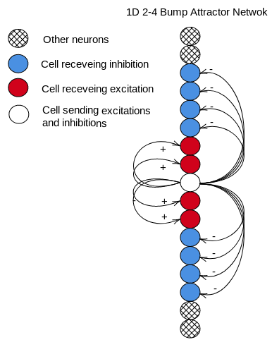
Figure 1. Minimal topology of a 1D bump attractor network with 2 positive connections (excitatory synapses) and 4 negative connections (inhibitory synapses). Given a neuron, it sends excitation to the two nearest top and bottom neurons and inhibition to the four subsequent top and bottom neurons.

Given N neurons, the connectivity matrix of a 1D 2-4 bump-attractor network is a squared matrix $A_{n,m}\in\mathbb{R}$ with $n=m=N$:

(1) $$A_{n,m}=\begin{pmatrix}a_{1,1}&a_{1,2}&\cdots&a_{1,m}\\ a_{2,1}&a_{2,2}&\cdots&a_{2,m}\\ \vdots&\vdots&\ddots&\vdots\\ a_{n,1}&a_{n,2}&\cdots&a_{n,m}\end{pmatrix}$$

where $a_{n,m}$ is equal to 1 if it represents a positive weight (excitatory synapse) or -1 if it represent a negative weight (inhibitory synapse). Note that $a_{n,m}$ is equal to 0 when there are no connections: in case of the 2-4 topology of the bump-attractor network are self connections or connections beyond the 2-4 boundary. Figure 2 shows an example of a connectivity matrix for a bump-attractor network having 2-4 topology with 20 neurons.

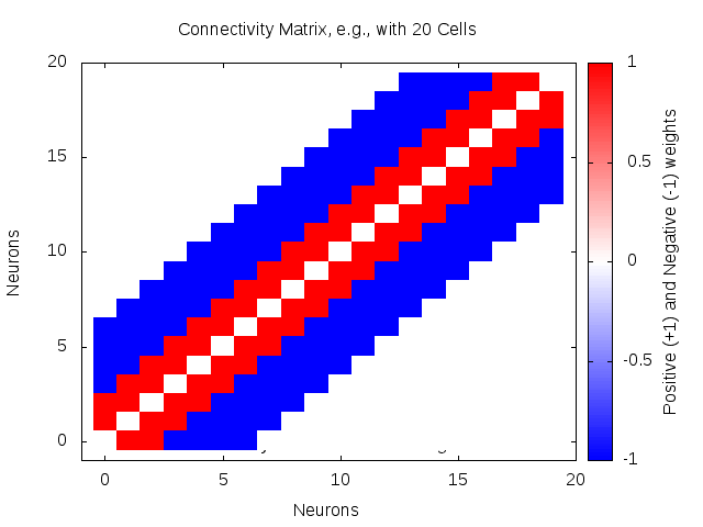
Figure 2. Connectivity matrix for a 1D bump attractor network of 20 cells. The weights are represented with unitary values, e.g., positive weights equal to 1 and negative weights equal to -1.

.

This work explores the number of weights range from 0.05 to 0.10 (step equal to 0.01). The combinationS between positive and negative weights is $6\times 6=36$. The input windows of spike sources range from 30 to 70 (step equal to 1), obtaining in total $70-30=40$ possible firing inputs. Therefore, there are $36\times 40=1440$ connectivity matrices.

The next section describes the neuronal model selected for the bump-attractor network and the hardware architecture adopted to run the experiments.

3. Simulations

The computations has been made selecting first a neuronal model to use in the bump-attractor network (Subsection 3.1) and then running the simulation in a dedicated neuromorphic environment (Subsection 3.2).

3.1. The neuronal model

The model of the biological neuron used in the simulation is the leaky integrate and fire model with a fixed threshold. Synaptic conductance is transmitted at a decaying-exponential rate from the pre to post-synaptic neurons (gerstner2014neuronal, ). The mathematical description of the model follows the work of Fourcaud (fourcaud2003spike, ) (see also (richardson2003conductance, ; gewaltig2007nest, )).

Equation 2 describes the temporal changes of the potential. The activation is the membrane potential $V_{M}$ and $C_{M}$ is the membrane capacity. The four currents are the leak current, the currents from excitatory and inhibitory synapses, and the input current (from an external spike source). The variable currents are governed by equations 3, 4 and 5. In equations 3 and 4 $E^{rev}_{Ex}$ and $E^{rev}_{In}$ are the reversal potentials; excitation and inhibition change slow as the voltage approaches these reversal potentials. In equation 5, $V_{rest}$ is the resting potential of the neuron, and $\tau_{M}$ is the leak constant.

(2) $$\frac{dV_{M}}{dt}=\frac{(-I_{Leak}-I^{syn}_{Ex}-I^{syn}_{In}+I_{Ext})}{C_{M}}$$

(3) $$I^{syn}_{Exc}=G_{Ex}\times(V_{M}-E^{rev}_{Ex})$$

(4) $$I^{syn}_{Inh}=G_{In}\times(V_{M}-E^{rev}_{In})$$

(5) $$I_{Leak}=\frac{C_{M}\times(V_{M}-V_{rest})}{\tau_{M}}$$

(6) $$G_{Ex}(t)=k_{Ex}\times t\times e^{-\frac{t}{\tau^{syn}_{Ex}}}$$

(7) $$G_{In}(t)=k_{In}\times t\times e^{-\frac{t}{\tau^{syn}_{In}}}$$

In the Equations 6 and 7, the $G_{Ex}$ and $G_{In}$ are the conductance in siemens to scale the post-synaptic potential amplitudes used in equation 3 and 4. $t$ is the time step.

The constant $k_{Ex}$ and $k_{In}$ are chosen so that $G_{Ex}(\tau^{syn}_{Ex})=1$ and $G_{In}(\tau^{syn}_{In})=1$. The $\tau^{syn}_{Ex}$ and the $\tau^{syn}_{In}$ are the decay rate of excitatory and inhibitory synaptic current.

When the voltage reaches the threshold, there is a spike and the voltage is reset. No current is transferred during the refractory period. In these simulations $v_{thresh}=-48.0$mV, $\tau_{refract}=2.0$ ms. The time step $t$ is 1ms. $C_{M}=1.0$nF, $v_{reset}=-70.0$mV, $v_{rest}=-65.0$mV, $E^{rev}_{Ex}=0.0$mV, $E^{rev}_{In}=-70$mV, $\tau^{syn}_{Ex}=5.0$ms, $\tau^{syn}_{In}=5.0$ms and $\tau_{M}=20.0$ms. These are all the default values. The particular parameters $v_{thresh}$,$\tau_{refract}$, and $t$, were selected as the authors have used them for prior simulations.

3.2. The computational setting

The bump-attractor network of leaky integrate and fire neurons has been implemented on SpiNNaker neuromorphic hardware (furber2014spinnaker, ). The whole SpiNNaker system is a spiking neural network architecture designed to deliver a massively parallel million-core computer whose interconnecting architecture is inspired by the connectivity characteristics of the mammalian brain. For the purpose of this paper, we adopted the 4-chip board that has 72 ARM processor cores, which will typically be deployed as 64 application cores, 4 Monitor Processors and 4 spare cores. The simulations are run with PyNN (davison2007pynn, ) to specify the topology, model, type of inputs, and recording of neuronal states.

Given the experimental conditions described in the above sections, the computational experiments is describable with the following pipeline:

• set-up the topology of a 1D bump-attractor network (2-4 connectivity) with 100 cells;

• simulation of the bump-attractor network dynamics given a specified set of deterministic spike sources, ranging from 1 to 40 inputs, using a unitary step; in other words, the window of inputs is from 1 spike source (window 31-30=1) to 40 spike sources (window 70-30=40).

• the computational run-time used is 300ms;

• simulations have been run with a different combination of positive and negative weights, varying from 0.05 to 0.10 (step equal to 0.01);

• the questions that are investigated are 1) if the network ignites and 2) if it does, do the spike trains have either a stable persistence, a splitting shape or a divergent pattern?;

• in particular, the splitting spike behaviour has been evaluated taking into account the number of streams, i.e., 2, 3 and 4, and the possible combination with the divergence pattern.

The next section presents the results achieved.

(a)

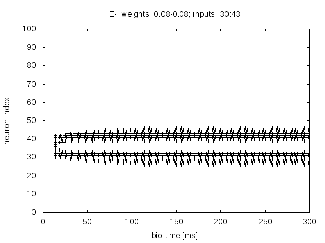
(b)

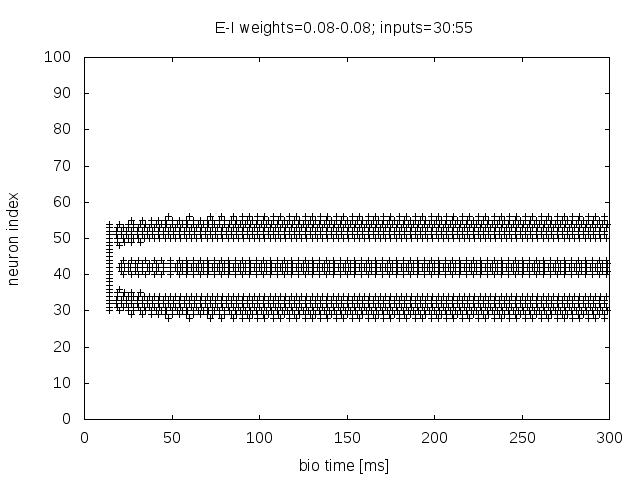
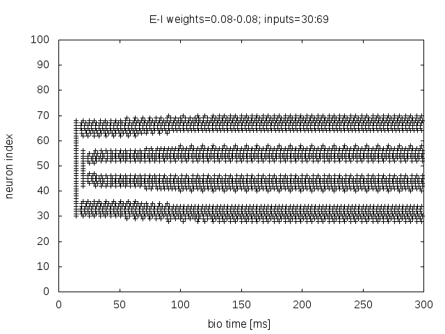
(c) (d)

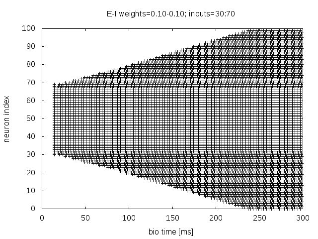
(e)

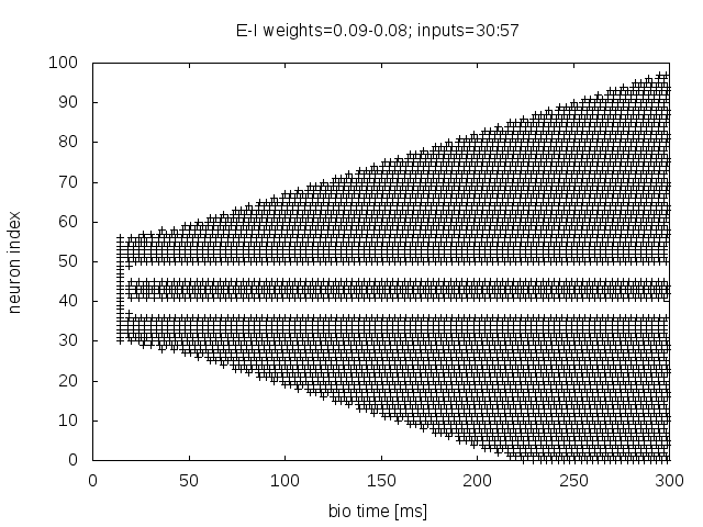
(f)

Figure 3. The figure shows the six different spike train patterns obtained with the simulations of a bump attractor network having different width of window inputs and positive and negative weight combinations. The (a) plot is stationary persistence of spikes. The (b) plot is the splitting behaviour with two streams of spikes. The (c) is the splitting with three streams. The (d) plot is the splitting with four streams. The (e) is the diverging spike train pattern. The (f) is the splitting behaviour with divergence. See also Figure 4 to see the relative voltage potential variations.

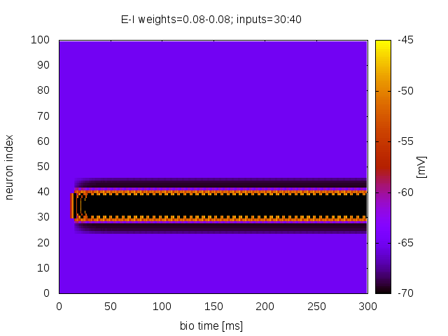
(a)

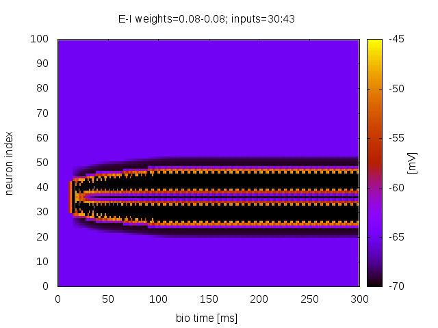
(b)

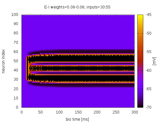
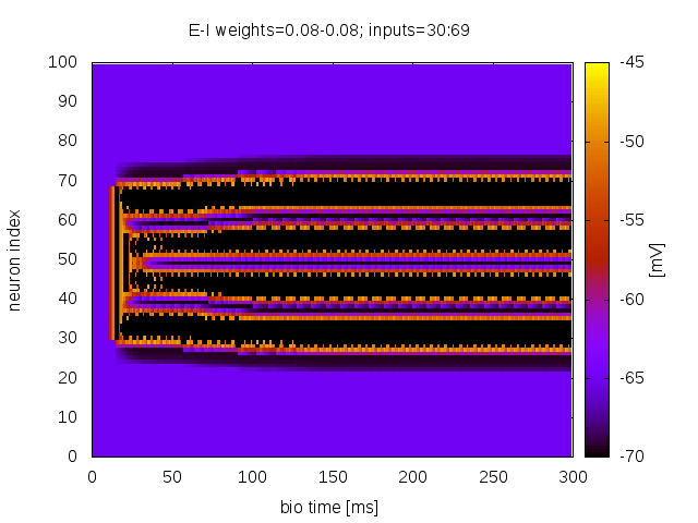
(c) (d)

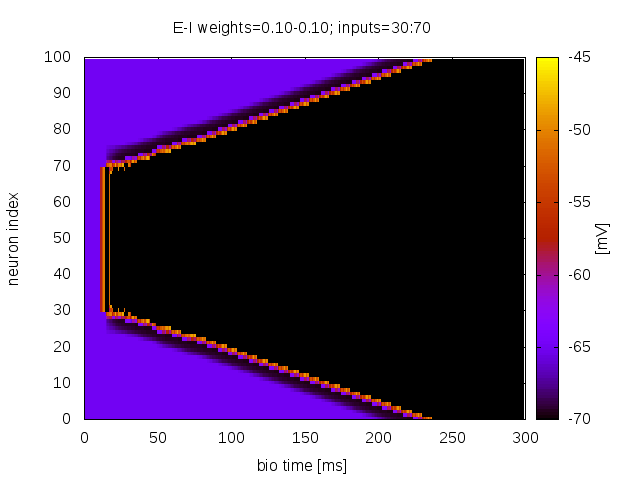
(e)

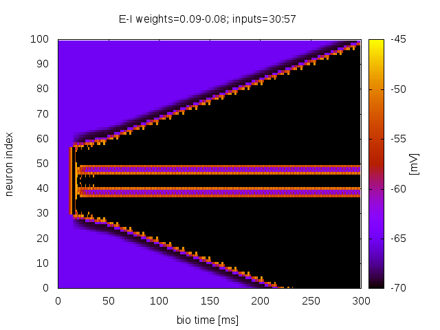
(f)

Figure 4. The figure shows the voltage potential variability associated to the six different spike train patterns obtained with the simulations of a bump attractor network having different size of window inputs and positive and negative weight combinations. The (a) plot is stationary persistence of spikes. The (b) plot is the splitting behaviour with two streams of spikes. The (c) is the splitting with three streams. The (d) plot is the splitting with four streams. The (e) is the diverging spike train pattern. The (f) is the splitting behaviour with divergence. See also Figure 3 to look the relative spike trains variations.

4. Results

The outcome of the simulations show the minimal number of input sources able to ignite the bump attractor system, and the critical number of input sources that produce the splitting behaviour of the spike trains into 2, 3 and 4 streams. An overview of the spike patterns of the bump attractor are shown in Figure 3 (with the relative voltage potential representation in Figure 4).

Table 1 shows the minimal numbers of spike sources able to ignite the bump attractor network, in relation to the different weights combinations, that are 1, 2, 4 and 5. The weight combinations related to 1 input are the ones with the highest excitatory weight (0.10) and all the range of inhibitory weights (0.05-0.10). The ignition of the network with 2 inputs is associated with the coupling of many excitatory weights (0.06-0.09) with all inhibitory weights (0.05-0.10). The lowest excitatory weight (0.05) combined with nearly all the inhibitory weights (0.05-0.09) allows the ignition mostly with 4 and 5 inputs. In the case of lowest excitatory weight (0.05) with the highest inhibitory weights (0.10) there is no network ignition even with 40 inputs.

	0.05	0.06	0.07	0.08	0.09	0.1
0.05	4	4	4	4	5	/
0.06	2	2	2	2	2	2
0.07	2	2	2	2	2	2
0.08	2	2	2	2	2	2
0.09	2	2	2	2	2	2
0.1	1	1	1	1	1	1

Table 1. Minimal number of spikes sources to ignite the 2-4 bump-attractor network. The $``/"$ means absence of any spikes.

	0.05	0.06	0.07	0.08	0.09	0.1
0.05	13	13	12	/	/	/
0.06	15	13	13	12	11	11
0.07	D	15	14	13	13	12
0.08	D	17(+D)	15(+D)	13	13	13
0.09	D	D	D	15(+D)	15(+D)	15
0.1	D	D	D	D	D	D

Table 2. Number of inputs that determine the splitting behaviour with 2 streams of the 2-4 bump attractor network. The $D$ means divergent behaviour and the $(+D)$ means that that splitting is combined with divergence, whereas $``/"$ means absence of any spikes.

Table 2 shows the critical cut-off of inputs that make the splitting behaviour of the bump net. The complete set of combination of excitatory and inhibitory weights ($6\times 6=36$) could be divided in three subsets: 1) the splitting subset, that has splitting behaviour of the spikes trains (no matter how many streams there are), 2) the divergent subset, that has divergent behaviour of the spike trains and 3) the null subset, that does not allow the network to persistently spike. Approximately, in Table 2, the splitting subset is in the upper right triangular part of the matrix, whereas the divergent subset is in the lower left triangular part of the matrix. The null subset of weights is within the last three elements (negative weights equal to 0.08, 0.09 and 0.10) of the first row (positive weight equal to 0.05).

The splitting subset in Table 2 encompasses the following E/I range: (0.05/0.05-0.07), (0.06/0.05-0.10), (0.07/0.06-0.10), (0.08/0.06-0.10) and (0.09/0.08-0.10). It is also sub-divisible in the weights combinations that allow the emergence of only two streams (Figure 3-b) and in the combinations that allow the emergence of three or four streams (see Figure 3-c and Figure 3-d). The subset with the divergent behaviour is the following positive and negative combination: (0.07/0.05), (0.08/0.06), (0.09/0.05-0.07) and (0.10/0.05-0.10). The patterns having divergent spikes trains have, globally, a common shape of divergence (see Figure 3-e).

E-I Weights	3S	4S
0.06-0.05	25	37
0.07-0.06	26	39
0.08-0.06	26 (+D)	na
0.08-0.07	23 (+D)	na
0.08-0.08	25	39
0.09-0.08	27 (+D)	na
0.09-0.09	25 (+D)	na

Table 3. Combination of excitatory E and inhibitory I weights that determine the splitting behaviour with 3 streams or 4 streams of the 2-4 bump attractor network. The $(+D)$ means that that splitting is combined with divergence and $``na"$ that the pattern is not present in the network configuration.

Table 3 shows the combinations of positive and negative weights that underlie the splitting phenomena with three streams and four streams, making also a differentiation if splits are merged with the divergent behaviour of the spike train patterns. For example the weights combination 0.08-0.08 generates the split with 3 streams with 25 (Figure 3-c) inputs and the split with 4 splits with 37 inputs (Figure 3-d), whereas the weights combination 0.09-0.08 generates only a split with 3 streams but also having divergence (see Figure 3-f to observe an example of divergence with streaming).

The next section considers the results achieved and some possible explanation of the different patterns of spike trains observed in the bump attractor network.

5. Discussion

This paper has explored some critical limits of the number of inputs sources in a bump attractor network. The criticality is related to the variability of the spike patterns that the system shows when the input window goes over or under a cut-off.

The principal results from this work regard 1) the minimal number of spike sources that allow the network to ignite, that is mostly around 2 input sources, excluding the extreme cases with the lowest (0.05) and highest (0.10) excitatory weights, and 2) the cut-off number of inputs sources that determines the splitting behaviour with two streams (see Figure 3-b), that ranges from 11 to 16, with a particular subset of weights combinations. Avoiding the case when the excitatory weights are 0.10, the streaming appears when the E/I weights are similar and - as a tendency - when the inhibitory weights are greater than excitatory weights (that are approximately the upper right triangular part of the Table 2)).

The stationary spiking pattern (Figure 3-a) emerges when the input sources window is over the minimal condition for the ignition and under the critical cut-off for the splitting with two streams (compare Table 1 with Table 2).

There is also a collection of weight combinations in the subset of the splitting behaviour, that enables the network to have spike patterns that split with 3 or 4 streams (see Table 3 and Figure 3-c/d). Note the when three streams are merged with the divergent behaviour (see Figure 3-f)). Instead, the whole divergence (see Figure 3-e)) appears in the complementary subset of weight combinations related to the splitting behaviour (approximately the lower left triangular part of the Table 2)

Observing the results obtained, it is possible to make the following considerations:

1. ignition can be achieved by a few inputs. It is not enough to ignite the network with only one spike source, except when the excitatory weight has high values, as 0.10 (see bottom row of Table 1);

2. the splitting behaviour with two streams is related to specific positive and negative weight combinations, that is when they are similar or with greater negative weights than the positive ones. Therefore, there could be a stronger role for inhibition in the context of streams genesis, rather than of excitation. To the contrary, the diverging behaviour of the spike train pattern seems to have a symmetric explanation, that is the greater role of excitation rather than the inhibition;

3. the subcases of spike train patterns with 3 and 4 streams and 3 streams with divergence seems related to the size of the input window. For instance, the number of streams grows as the number of spike sources increases; therefore the more inputs ignite the bump network, the more (could be) the streams within the splitting behaviour (see Table 3);

4. the other subcases of streaming with divergence could be described as particular weight combination, related to a specific input size, that share both the property of divergence and splitting behaviour for the bump network. In particular, the combination of weights that determine the streaming with divergence are collocated in the boundary between the weight condition underlying the splitting and the divergent behaviour of the spike trains. Therefore, the merged splits and divergence seems an intermediate situation of the weights combination close to both the pattern possibilities.

These results have some limitations. First of all, the topology of the bump attractor network has 2-4 positive-negative synaptic connections. Given a neuron, it has excitatory synapses to the nearest two cells (top and bottom) and inhibitory connections with the following four cells (top and bottom) (see Figure 1). Furthermore, it is a one dimensional network with 100 neurons. A realistic bump attractor has a relative larger size with a more flexible positive-negative connection ratio. An example of an anatomical persistent bump attractor is the head direction cells since their activity does not stop when the light is turned off and the bump is stable in the absence of input (gerstner2014neuronal, ). In this case, the stimuli or the memory recall operation drives the initial perturbation of the localized blob of activity, that is a biological bump attractor. Another example is from the study related to the prefrontal cortex where the prefrontal persistent activity during the delay of spatial working memory tasks is thought to maintain spatial location in memory. There are recent results in monkey studies (see work by Wimmer et al (wimmer2014bump, )) that support a diffusing bump representation for spatial working memory instantiated in persistent prefrontal activity.

Another limitation is related to the combinatorial exploration of a predefined set of positive and negative weights coupling, without using any learning rule, they are basically static weights. In a realistic bump attractor, there are natural learning strategies, e.g., the Hebbian rule (hebb1949, ), that govern the weight states in real time.

Future works will investigate the critical limits of the bump attractor network taking into account a more realistic configuration of the topology. Natural learning rules or other weight combinations could be used. This work adopted a particular leaky integrate and fire model (gerstner2014neuronal, ), but other simulations could regard different neuronal models with other parameter configurations. Regarding the measurement of state variables, this research focused only on the spike trains and on the voltage membrane potentials without measuring other quantities or deriving interesting ones.

Further analysis should be done taking account also that the bump attractor network is an example of a dynamical system (Meiss:2007, ; Terman:2008, ). The next computational explorations of the network behaviours should encompass a deeper understanding of those emerging patterns from the theoretical perspective of the physics of complex systems (Nicolis:2007, ), applied in the context of the neuronal modelling and simulation by using both standard software environment for brain simulations (e.g. NEST (gewaltig2007nest, )) and neuromorphic computing architectures (e.g., SpiNNaker (Furber, ) and other systems (schuman2017survey, )).

References

- (1) Chen, Y. Mechanisms of winner-take-all and group selection in neuronal spiking networks. Frontiers in computational neuroscience 11 (2017), 20.
- (2) Davison, A., Yger, P., Kremkow, J., Perrinet, L., and Muller, E. Pynn: towards a universal neural simulator api in python. BMC neuroscience 8, S2 (2007), P2.
- (3) Edelman, G. M. Neural Darwinism: The theory of neuronal group selection. Basic books, 1987.
- (4) Eliasmith, C. Attractor network. Scholarpedia 2, 10 (2007), 1380. revision #91016.
- (5) Fourcaud-Trocmé, N., Hansel, D., Van Vreeswijk, C., and Brunel, N. How spike generation mechanisms determine the neuronal response to fluctuating inputs. Journal of Neuroscience 23, 37 (2003), 11628–11640.
- (6) Furber, S., Lester, D., Plana, L., Garside, J., Painkras, E., Temple, S., and Brown, A. Overview of the spinnaker system architecture. IEEE Transactions on Computers 62, 12 (2013), 2454–2467.
- (7) Furber, S. B., Galluppi, F., Temple, S., and Plana, L. A. The spinnaker project. Proceedings of the IEEE 102, 5 (2014), 652–665.
- (8) Gerstner, W., and Brette, R. Adaptive exponential integrate-and-fire model. Scholarpedia 4, 6 (2009), 8427. revision #90944.
- (9) Gerstner, W., Kistler, W. M., Naud, R., and Paninski, L. Neuronal dynamics: From single neurons to networks and models of cognition. Cambridge University Press, 2014.
- (10) Gewaltig, M., and Diesmann, M. Nest (neural simulation tool). Scholarpedia 2, 4 (2007), 1430.
- (11) Hebb, D. O. The Organization of Behavior: A Neuropsychological Theory. J. Wiley & Sons, 1949.
- (12) Koroutchev, K., and Korutcheva, E. Improved storage capacity of hebbian learning attractor neural network with bump formations. In International Conference on Artificial Neural Networks (2006), Springer, pp. 234–243.
- (13) Laing, C., R., Chow, and Carson, C. Stationary bumps in networks of spiking neurons. Neural computation 13, 7 (2001), 1473–1494.
- (14) Maass, W. On the computational power of winner-take-all. Neural computation 12, 11 (2000), 2519–2535.
- (15) Meiss, J. Dynamical systems. Scholarpedia 2, 2 (2007), 1629. revision #137210.
- (16) Nicolis, G., and Rouvas-Nicolis, C. Complex systems. Scholarpedia 2, 11 (2007), 1473. revision #91143.
- (17) Richardson, M. J., and Gerstner, W. Conductance versus current-based integrate-and-fire neurons: Is there qualitatively new behaviour? Lausanne lecture (2003).
- (18) Schuman, C. D., Potok, T. E., Patton, R. M., Birdwell, J. D., Dean, M. E., Rose, G. S., and Plank, J. S. A survey of neuromorphic computing and neural networks in hardware. arXiv preprint arXiv:1705.06963 (2017).
- (19) Seeholzer, A., Deger, M., and Gerstner, W. Stability of working memory in continuous attractor networks under the control of short-term plasticity. PLoS computational biology 15, 4 (2019), e1006928.
- (20) Somers, D. C., Nelson, S. B., and Sur, M. An emergent model of orientation selectivity in cat visual cortical simple cells. Journal of Neuroscience 15, 8 (1995), 5448–5465.
- (21) Terman, D. H., and Izhikevich, E. M. State space. Scholarpedia 3, 3 (2008), 1924. revision #137545.
- (22) Wilson, H. R., and Cowan, J. D. A mathematical theory of the functional dynamics of cortical and thalamic nervous tissue. Kybernetik 13, 2 (1973), 55–80.
- (23) Wimmer, K., Nykamp, D. Q., Constantinidis, C., and Compte, A. Bump attractor dynamics in prefrontal cortex explains behavioral precision in spatial working memory. Nature neuroscience 17, 3 (2014), 431.