Performance of quantum heat engines under the influence of long-range interactions

Abstract

We examine a quantum heat engine with an interacting many-body working medium consisting of the long-range Kitaev chain to explore the role of long-range interactions in the performance of the quantum engine. By analytically studying two types of thermodynamic cycles, namely, the Otto cycle and Stirling cycle, we demonstrate that the work output and efficiency of a long-range interacting heat engine can be boosted by the long-range interactions, in comparison to the short-range counterpart. We further show that in the Otto cycle there exists an optimal condition for which the maximum enhancement in work output and efficiency can be achieved simultaneously by the long-range interactions. But, for the Stirling cycle, the condition which can give the maximum enhancement in work output does not lead to the maximum enhancement in efficiency. We also investigate how the parameter regimes under which the engine performance is enhanced by the long-range interactions evolve with a decrease in the range of interactions.

I introduction

Since the seminal work of Scovil and Schulz-DuBois Scovil and Schulz-DuBois (1959), the concept of quantum heat engines has attracted lots of attention Alicki (1979); Geva and Kosloff (1992); Scully et al. (2003); Kieu (2004); Quan et al. (2005, 2006); Henrich et al. (2007); Quan et al. (2007); Quan (2009); Kosloff and Levy (2014). In particular, in the last few decades, spurred by experimental and theoretical progress in the field of quantum thermodynamics (see, e. g., Refs. Binder et al. (2018); Vinjanampathy and Anders (2016); Deffner and Campbell (2019) and references therein), a tremendous amount of effort has been devoted to studies of quantum heat engines, both experimentally Koski et al. (2014); Roßnagel et al. (2016); Klaers et al. (2017); Zou et al. (2017); Klatzow et al. (2019); de Assis et al. (2019); von Lindenfels et al. (2019); Peterson et al. (2019) and theoretically Roßnagel et al. (2014); Gelbwaser-Klimovsky et al. (2015); Uzdin et al. (2015); Abiuso and Perarnau-Llobet (2020); Kosloff and Rezek (2017); Deffner and Campbell (2019). As the quantum versions of classical engines, quantum heat engines exploit quantum systems as their working medium to extract work in quantum thermodynamic cycles Kieu (2004); Quan et al. (2007). A wide range of quantum systems have been used to devise quantum heat engines, including harmonic oscillators Kosloff and Rezek (2017); Insinga et al. (2016); Reid et al. (2017), spin systems Thomas and Johal (2011); Altintas and Müstecaplıoğlu (2015); Campisi et al. (2015); Marchegiani et al. (2016); Barrios et al. (2017); Hewgill et al. (2018), photons Scully et al. (2003); Dillenschneider and Lutz (2009), optomechanical systems Zhang et al. (2014a), Dirac particles Muñoz and Peña (2012); Peña et al. (2016), and quantum dots Josefsson et al. (2018); Peña et al. (2019, 2020). A few works have also considered quantum engines with the heat reservoirs replaced by quantum systems Roßnagel et al. (2014); Zhang et al. (2014b); Niedenzu et al. (2018).

Numerous studies in quantum heat engines are focused on possible enhancement in work output and efficiency via the utilization of quantum properties in various working mediums Hardal and Müstecaplıoğlu (2015); Hewgill et al. (2018); Van Horne et al. (2018); Watanabe et al. (2017) or heat reservoirs Scully et al. (2003); Roßnagel et al. (2014); Klaers et al. (2017); Niedenzu et al. (2018). Other efforts are towards understanding the fundamental differences between classical and quantum heat engines Quan et al. (2007); Gardas and Deffner (2015); Friedenberger and Lutz (2017), finite time cycles Esposito et al. (2010); Feldmann and Kosloff (2012); Wu et al. (2014); Zheng et al. (2016); Cavina et al. (2017); Wiedmann et al. (2019), and the applications of shortcuts to adiabaticity Deng et al. (2013); Campo et al. (2014); Li et al. (2018); Abah and Lutz (2018, 2018); Abah and Paternostro (2019); Çakmak and Müstecaplıoğlu (2019); Funo et al. (2019); Hartmann et al. (2019). The effects of quantum statistics on the performance of quantum heat engines have also been investigated Zheng and Poletti (2015); Watanabe et al. (2019). Very recently, the results in Ref. Myers and Deffner (2020) further demonstrated that wave-function symmetry has nontrivial impacts on the performance of quantum heat engines.

Most of the aforementioned works are limited to the single or few-particle working mediums. However, with the aim to scale up quantum heat engines and related thermodynamic devices, it is necessary for us to consider many-body quantum heat engines. Several recent studies have reported that engine performance can be enhanced by various quantum many-body effects, such as quantum phase transitions Campisi and Fazio (2016); Ma et al. (2017); Fadaie et al. (2018); Kloc et al. (2019); S. et al. (2020) and many-body localization Yunger Halpern et al. (2019). Importantly, the significant role played by interparticle interactions in quantum many-body heat engines has been revealed in Refs. Jaramillo et al. (2016); Beau et al. (2016); Chen et al. (2019).

On the other hand, the recent experimental realization of quantum many-body systems with tunable long-range interactions Jurcevic et al. (2014); Richerme et al. (2014) has triggered a surge of interest in the properties of quantum systems with long-range interactions Santos et al. (2016); Halimeh and Zauner-Stauber (2017); Gong et al. (2017); Jaschke et al. (2017); Žunkovič et al. (2018); Liu et al. (2019); Lerose et al. (2019); Piccitto et al. (2019); Puebla et al. (2019); Sierant et al. (2019). In these systems, the interaction strength between two particles with distance $r$ usually decays as $1/r^{\alpha}$ with $\alpha\geq 0$. Due to the long-range interactions, long-range interacting systems can host novel features that are not observed in their short-range counterparts, such as the anomalous dynamical phase Homrighausen et al. (2017), the quantum time crystal without an external driver Kozin and Kyriienko (2019), and the breakdown of locality (see Refs. Liu et al. (2019); Schachenmayer et al. (2013); Buyskikh et al. (2016) and references therein). Given the fact that the long-range interactions are very relevant in experimental platforms that include Rydberg atoms Saffman et al. (2010), trapped ions Jurcevic et al. (2014); Richerme et al. (2014); Britton et al. (2012); Islam et al. (2013), polar molecules Bohn et al. (2017), and magnetic atoms Lahaye et al. (2009), it is thus interesting to see whether the long-range interactions can be used to enhance engine performance.

In this work we explore the enhancement effect of long-range interactions on the performance of a quantum heat engine which employs the long-range Kitaev chain as its working medium. The long-range Kitaev chain can be considered an extension of the well-known Kitaev chain Kitaev (2001) with a long-range superconducting pairing term and has been used as a prototypical model in the studies of long-range interacting systems Vodola et al. (2014); Vodola (2015); Maity et al. (2019). By exploiting the integrability of the long-range Kitaev chain, we are able to obtain the explicit expressions for the work output and efficiency of the quantum engine. We will consider two types of thermodynamic cycles, namely, the Otto cycle and Stirling cycle, respectively. For both types of cycles, we find that the long-range interactions can display a notable improvement in engine performance in comparison to the case of short-range interactions. We further demonstrate how the enhancement regions in the cycle parameter space evolve with the range of interactions. Here we stress that we consider only the quasistatic cycles, leaving the cycles that operate in finite time as an interesting topic of future study. Moreover, we focus on the engine performance in terms of work output and efficiency.

The remainder of this article is organized as follows. In Sec. II we introduce the long-range interacting Kitaev chain and review briefly some of its basic features; we also specify the exact expressions for the thermodynamic quantities of the long-range Kitaev chain in this section. In Sec. III we describe two types of thermodynamic cycles (i. e., the Otto cycle and the Stirling cycle) in which our quantum heat engine operates and we extract the analytical expressions for work output and the efficiency of these cycles, respectively. Then we present our numerical results and a discussion in Sec. IV. We finally conclude our study in Sec. V.

II The long-range Kitaev Chain

We consider the one-dimensional Kitaev model with long-range pairing interactions. Its Hamiltonian reads Vodola et al. (2014); Pezzè et al. (2017); Maity et al. (2019); Vodola (2015); Dutta and Dutta (2017)

$$H= -J\sum_{j=1}^{L}(c_{j}^{\dagger}c_{j+1}+c_{j+1}^{\dagger}c_{j})-\mu\sum_{j=1}^{L}\left(c_{j}^{\dagger}c_{j}-\frac{1}{2}\right)$$

$$+\frac{\Delta}{2}\sum_{j=1}^{L}\sum_{\ell=1}^{L-1}\frac{1}{d_{\ell}^{\alpha}}\left(c_{j}c_{j+\ell}+c_{j+\ell}^{\dagger}c_{j}^{\dagger}\right).$$ (1)

Here, $c_{j}^{\dagger}(c_{j})$ are the fermionic creation (annihilation) operators on the $j$th site, $L$ denotes the size of the model, and $\mu$ is the on-site chemical potential. $J$ represents the hopping strength of the fermion between nearest neighbor sites, while $\Delta$ is the strength of the fermion pairing interactions. The power-law decaying pairing term is characterized by the exponent $\alpha$. $d_{\ell}=\mathrm{min}(\ell,L-\ell)$ is the effective distance between the $i$th and $(i+\ell)$th sites. In our study, we consider a close chain with an antiperiodic boundary condition $c_{j}=-c_{j+L}$ and assume the total number of sites $L$ is even. Throughout this work, we set $\hbar=1$.

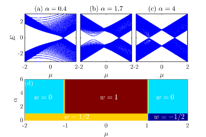
Figure 1: Energy spectrum as a function of $\mu$ of the long-range Kitaev chain (II) with antiperiodic boundary condition for (a) $\alpha=0.4$, (b) $\alpha=1.7$, and (c) $\alpha=4$. The system size is $L=200$, $J=\Delta=1$, and $\hbar=1$. (d) Schematic phase diagram of the long-range Kitaev chain in the $\mu-\alpha$ plan. Different phases are indicated by different colors with corresponding winding number $w$. All quantities are unitless.

In the short-range limit $\alpha\to\infty$, the Hamiltonian in Eq. (II) reduces to the well-known short-range Kitaev chain Kitaev (2001), which can be mapped to the quantum transverse field Ising model via the Jordan-Wigner transformation Lieb et al. (1961). In this case, by analytically diagonalizing the Hamiltonian, one can find that the model undergoes the topological phase transitions at the critical points $\mu/J=\pm 1$. For finite $\alpha$, the above-mentioned mapping does not exist anymore. However, the quadratic form of the Hamiltonian (II) implies that it can still be exactly diagonalized for any finite $\alpha$.

To this end, we first recast the Hamiltonian (II) in the momentum space via the Fourier transform $c_{j}=L^{-1/2}\sum_{k}c_{k}e^{-ikj}$, where due to an antiperiodic boundary condition, the lattice momentum $k=\pm\pi(2n-1)/L$ with $n=1,2,\ldots,L/2$. Then the Hamiltonian takes the following block diagonal form Maity et al. (2019); Pezzè et al. (2017); Dutta and Dutta (2017)

$$H=\sum_{k}\mathcal{C}^{\dagger}_{k}\mathcal{H}_{k}\mathcal{C}_{k},$$ (2)

where $\mathcal{C}_{k}^{\dagger}=(c_{k}^{\dagger},c_{-k})$ and

$$\mathcal{H}_{k}=\begin{bmatrix}-(J\cos k+\mu)&i\Delta f_{\alpha}(k)/2\\ -i\Delta f_{\alpha}(k)/2&J\cos k+\mu\end{bmatrix},$$ (3)

with the function $f_{\alpha}(k)=\sum_{\ell=1}^{L-1}\sin(k\ell)/d_{\ell}^{\alpha}$.

The Hamiltonian (2) can be diagonalized through the Bogoliubov transformation

$$\begin{pmatrix}c_{k}\\ c_{-k}^{\dagger}\end{pmatrix}=\begin{pmatrix}\cos\theta_{k}&i\sin\theta_{k}\\ i\sin\theta_{k}&\cos\theta_{k}\end{pmatrix}\begin{pmatrix}d_{k}\\ d_{-k}^{\dagger}\end{pmatrix}.$$ (4)

Here, the Bogoliubov angle $\theta_{k}$ is defined as

$$\tan(2\theta_{k})=-\frac{\Delta f_{\alpha}(k)/2}{J\cos k+\mu}.$$ (5)

The Hamiltonian (II) is finally diagonalized as

$$H=\sum_{k}\varepsilon_{k}\left(d^{\dagger}_{k}d_{k}-\frac{1}{2}\right),$$ (6)

where $\varepsilon_{k}$ is the quasiparticle energy and is given by

$$\varepsilon_{k}=\sqrt{(J\cos k+\mu)^{2}+[\Delta f_{\alpha}(k)/2]^{2}}.$$ (7)

For the short-range limit $\alpha\to\infty$, we have $f_{\infty}(k)=2\sin k$ Maity et al. (2019); Pezzè et al. (2017). Then the quasiparticle energy $\varepsilon_{k}$ takes the usual short-range form Kitaev (2001). However, in the thermodynamic limit $L\to\infty$, the function $f_{\alpha}(k)$ becomes $f_{\alpha}^{\infty}(k)=(-i/2)\left[\mathbf{Li}_{\alpha}(e^{ik})-\mathbf{Li}_{\alpha}(e^{-ik})\right]$, with $\mathbf{Li}_{\alpha}(x)=\sum_{\ell=1}^{\infty}(x^{\ell}/\ell^{\alpha})$ being the $\alpha$th-order polylogarithm function of $x$ Pezzè et al. (2017); Dutta and Dutta (2017); Maity et al. (2019); Vodola (2015). It is known that for $\alpha>1$, $f_{\alpha}^{\infty}(k)$ vanishes at $k=0$ and $k=\pi$, while when $\alpha<1$, $f_{\alpha}^{\infty}(k)=0$ occurs only at $k=\pi$ Pezzè et al. (2017); Maity et al. (2019); Dutta and Dutta (2017). Thus for finite $\alpha$, the spectrum is gapless at $\mu/J=\pm 1$ when $\alpha>1$, whereas once $\alpha<1$, we have $\varepsilon_{k}=0$ only at $\mu/J=1$. For brevity but without loss of generality, we set $J=\Delta=1$ in the following part of our study.

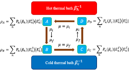
Figure 2: Schematic diagram of the quantum Otto cycle studied in this work. The thermodynamic cycle operats between a hot bath at temperature $\beta_{h}^{-1}$ and a cold bath at temperature $\beta_{c}^{-1}$. It consists of two adiabatic ($A\to B$ and $C\to D$) and two isochoric ($B\to C$ and $D\to A$) strokes. $\mu_{i}$ and $\mu_{f}$ are the chemical potential in the two isochoric strokes. $\rho_{\gamma}$ ($\gamma=A,B,C,D$) denotes the state of the working medium at each stage of the cycle. At stages $A$ and $C$ the working medium is in thermal equilibrium with the hot and cold baths, respectively.

For the long-range Kitaev chain with antiperiodic boundary conditions, the energy spectrum with respect to the different chemical potential $\mu$ for several values of $\alpha$ is plotted in panels (a)–(c) of Fig. 1. Clearly, regardless of $\alpha$, the energy gap is always close to zero at $\mu=1$. In contrast, the gap at $\mu=-1$ is increased with decreasing $\alpha$. In the thermodynamic limit $L\to\infty$, one can expect that the energy gap closes at $\mu=\pm 1$ for $\alpha>1$, while it closes only at $\mu=1$ when $\alpha<1$. The close of the energy gap in the spectrum corresponds to the transitions between different topological phases, which are characterized by different winding numbers. The winding number is defined as $w=(1/2\pi)\int_{-\pi}^{\pi}(\partial_{k}\theta_{k})dk$, with $\theta_{k}$ the Bogoliubov angle given by Eq. (5). Figure 1(d) shows the schematic phase diagram of the long-range Kitaev chain in the $\mu-\alpha$ plan. The topological phases with different winding numbers are discriminated by different color regions. Depending upon the values of $\mu$ and $\alpha$, distinct topological phases with $w=\pm 1/2,0,1$ are displayed in the model. It is worth mentioning that the effects of the topological phase transition on the work and efficiency of the quantum heat engine have been explored in Refs. Fadaie et al. (2018); Yunt et al. (2019). In our study we mainly focus on the influences of the long-range interactions on the performance of quantum heat engines. Moreover, in order to avoid the divergence in thermodynamic limit for $0\leq\alpha\leq 1$, we restrict our study to $\alpha>1$, as is done in other studies of long-range interacting systems Liu et al. (2019); Dutta and Dutta (2017).

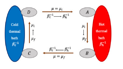
Figure 3: Graphic sketch of the quantum Stirling cycle operating between two thermal baths (hot and cold) at temperatures $\beta_{h}^{-1}$ and $\beta_{c}^{-1}$, respectively. The cycle has two isothermal ($A\to B$ and $C\to D$) and two isochemical ($B\to C$ and $D\to A$) potential processes. $\mu_{i}$ and $\mu_{f}$ are the values of the chemical potential in the two isochemical potential processes.

Expressions of the thermodynamic quantities

Considering the model is in an equilibrium state at temperature $\beta^{-1}$, here and henceforth we set $k_{B}=1$. The state of the model is, therefore, the Gibbs state $\rho=e^{-\beta H}/\mathcal{Z}$, where $\mathcal{Z}=\mathrm{tr}(e^{-\beta H})$ is the partition function. This, of course, assumes that the energy of the system is the only conserved quantity and the thermodynamics of the system is calculated by the standard Gibbs measure. From the diagonal form of the Hamiltonian in Eq. (6), the partition function can be written as

$$\mathcal{Z}=2^{L}\prod_{k>0}\cosh^{2}\left(\frac{\beta\varepsilon_{k}}{2}\right).$$ (8)

Then the internal energy $U$ and the free energy $F$ for the long-range Kitaev chain are respectively given by

$$U=\mathrm{tr}(\rho H)=-\frac{\partial\ln\mathcal{Z}}{\partial\beta}=-\sum_{k>0}\varepsilon_{k}\tanh\left(\frac{\beta\varepsilon_{k}}{2}\right),$$ (9)

$$F=-\frac{\ln\mathcal{Z}}{\beta}=-\frac{1}{\beta}\left[L\ln 2+\sum_{k>0}2\ln\cosh\left(\frac{\beta\varepsilon_{k}}{2}\right)\right].$$ (10)

With the density of state $\rho$, one can find the entropy $S=-\mathrm{Tr}[\rho\ln\rho]$ has the from

$$S=L\ln 2+\sum_{k>0}\left[2\ln\cosh\left(\frac{\beta\varepsilon_{k}}{2}\right)-\beta\varepsilon_{k}\tanh\left(\frac{\beta\varepsilon_{k}}{2}\right)\right].$$ (11)

Armed with these results, we turn to investigating the effects of the interacting range on the performance of the quantum heat engine.

III Thermodynamic cycles

In our study, we analyze the performance of a quantum heat engine with the long-range Kitaev chain in Eq. (II) as its working medium. We focus on two types of thermodynamic cycles, namely, the Otto cycle and Stirling cycle.

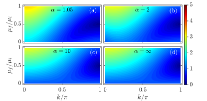
Figure 4: Quasiparticle energy $\varepsilon_{k}$ (7) as a function of $k$ (rescaled by $\pi$) and $\mu_{f}$ (rescaled by $\mu_{i}$) for different ranges of interactions: (a) $\alpha=1.05$, (b) $\alpha=2$, (c) $\alpha=10$, and (d) $\alpha=\infty$. Parameters are: $\hbar=k_{B}=1$, $J=\Delta=1$, $L=2000$, and $\mu_{i}=2$.

III.1 Quantum Otto cycle

As a widely used cycle in both theoretical and experimental studies of quantum heat engines, the quantum Otto cycle consists of two isochoric and two adiabatic strokes Henrich et al. (2007); Quan et al. (2007), see Fig. 2. In the isochoric branches, the working medium with fixed Hamiltonian is coupled to the hot and cold baths and thermalized with the baths. For the adiabatic strokes of the cycle, the working medium is detached from the hot and cold baths, and undergoes a unitary evolution by changing the control parameter in the Hamiltonian in an infinitely slow way so that the quantum adiabatic theorem holds. The details of the four strokes are described as follows.

(a) Adiabatic stroke $A\to B$ (expansion process). The working medium is initially in the thermal state $\rho_{A}=\sum_{n}P_{n}(\beta_{h})|E_{n}^{i}\rangle\langle E_{n}^{i}|$ at temperature $\beta_{h}^{-1}$ and Hamiltonian $H_{i}$, which gives by Eq. (II) with $\mu=\mu_{i}$. Here, $|E_{n}^{i}\rangle$ is the $n$th eigenstate of the Hamiltonian $H_{i}$ with corresponding eigenvalue $E_{n}^{i}$, and $P_{n}(\beta_{h})=e^{-\beta_{h}E_{n}^{i}}/\mathcal{Z}_{h}$ with $\mathcal{Z}_{h}=\sum_{n}e^{-\beta_{h}E_{n}^{i}}$. Then we decouple the working medium from the thermal bath and slowly vary the chemical potential from $\mu_{i}$ to $\mu_{f}$ ($\mu_{f}\leq\mu_{i}$) such that the quantum adiabatic theorem holds in this process. Hence, during the process the occupation probability of each eigenstate of the working medium remains the same; no heat is transferred. However, the change in the chemical potential $\mu$ results in the work being done in this process. At the end of the stroke, the working medium reaches the state $\rho_{B}=\sum_{n}P_{n}(\beta_{h})|E_{n}^{f}\rangle\langle E_{n}^{f}|$, where $\{|E_{n}^{f}\rangle\}$ are the eigenstates of $H_{f}$, which is the Hamiltonian (II) with $\mu=\mu_{f}$.

(b) Isochoric stroke $B\to C$ (cooling process). In this stroke, the chemical potential is fixed at $\mu=\mu_{f}$ and the working medium is brought in contact with the cold bath at temperature $\beta_{c}^{-1}$ until it attains the thermal equilibrium with the cold bath. The state of the working medium at the end of this process is, therefore, given by $\rho_{C}=\sum_{n}P_{n}(\beta_{c})|E_{n}^{f}\rangle\langle E_{n}^{f}|$, with $P_{n}(\beta_{c})=e^{-\beta_{c}E_{n}^{f}}/\mathcal{Z}_{c}$ and $\mathcal{Z}_{c}=\sum_{n}e^{-\beta_{c}E_{n}^{f}}$. Because the chemical potential is fixed, no work has been done in this process, and the heat $Q_{O}^{c}$ is ejected from the working medium to the cold bath.

(c) Adiabatic stroke $C\to D$ (compression process). The working medium is detached from the cold bath and the chemical potential is adiabatically driven back from $\mu_{f}$ to $\mu_{i}$. The occupation probability of each energy levels stays at the values $P_{n}(\beta_{c})$. The work is done in this process but no heat transfer. At the end of this stroke, the state of the working medium reads $\rho_{D}=\sum_{n}P_{n}(\beta_{c})|E_{n}^{i}\rangle\langle E_{n}^{i}|$.

(d) Isochoric stroke $D\to A$ (heating process). This is an isochoric heating process in which the working medium, with chemical potential $\mu=\mu_{i}$ and Hamiltonian $H=H_{i}$, is attached with the hot bath at temperature $\beta^{-1}_{h}$, relaxing to the thermal state $\rho_{A}$. In this process, the fixed chemical potential means that the energy levels are unchanged, no work is done. But the change in the occupation probability of each eigenstate causes the working medium to absorb heat $Q_{O}^{h}$ from the hot bath.

As no work is done in the two isochoric strokes of the cycle, the heat transfer between the working medium and the heat bath in the isochoric heating and cooling strokes is equal to the variation of internal energy during the processes. Therefore the heat $Q_{O}^{h}$ injected into the working medium in the heating stroke and heat $Q_{O}^{c}$ ejected in the cooling stroke are calculated as $Q_{O}^{h}=\mathrm{Tr}[H_{i}(\rho_{A}-\rho_{D})],Q_{O}^{c}=\mathrm{Tr}[H_{f}(\rho_{C}-\rho_{B})]$ Quan et al. (2007); Henrich et al. (2007); Thomas and Johal (2011). By using Eq. (9), one can explicitly write $Q_{O}^{h}$ and $Q_{O}^{c}$ as follows:

$$Q_{O}^{h} =\sum_{k>0}\varepsilon_{k}^{i}\left[\tanh\left(\frac{\beta_{c}\varepsilon_{k}^{f}}{2}\right)-\tanh\left(\frac{\beta_{h}\varepsilon_{k}^{i}}{2}\right)\right],$$ (12)

$$Q_{O}^{c} =\sum_{k>0}\varepsilon_{k}^{f}\left[\tanh\left(\frac{\beta_{h}\varepsilon_{k}^{i}}{2}\right)-\tanh\left(\frac{\beta_{c}\varepsilon_{k}^{f}}{2}\right)\right],$$ (13)

where $\varepsilon_{k}^{i}$ and $\varepsilon_{k}^{f}$ are given by Eq. (7), where $\mu$ is replaced by $\mu_{i}$ and $\mu_{f}$, respectively.

The work is done only in the quantum adiabatic strokes of the cycle. From the first law of thermodynamics, the amount of net work performed by the Otto cycle is given by

$$W_{O} =Q_{O}^{h}+Q_{O}^{c}$$

$$=\sum_{k>0}\left(\varepsilon_{k}^{i}-\varepsilon_{k}^{f}\right)\left[\tanh\left(\frac{\beta_{c}\varepsilon_{k}^{f}}{2}\right)-\tanh\left(\frac{\beta_{h}\varepsilon_{k}^{i}}{2}\right)\right].$$ (14)

Note that in order to make sure the cycle works as an engine, we must have $W_{O}>0$, $Q_{O}^{h}>-Q_{O}^{c}>0$. Then the efficiency of the engine is given by

$$\eta_{O}=\frac{W_{O}}{Q_{O}^{h}}.$$ (15)

It is known that the efficiency of the quantum Otto cycle is bounded by the Carnot efficiency $\eta_{c}=1-\beta_{h}/\beta_{c}$ Quan et al. (2007).

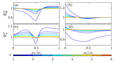
Figure 5: Left column: Work output ratio $\mathcal{R}_{W}^{O}$ (a) and the efficiency ratio $\mathcal{R}_{\eta}^{O}$ (c) of Otto cycle, see Eq. (23), as a function of $\mu_{f}/\mu_{i}$ for $\alpha\in[1.05,6]$ at $\beta_{c}=5$. Right column: $\mathcal{R}_{W}^{O}$ (b) and $\mathcal{R}_{\eta}^{O}$ (d) as a function of $\mu_{f}/\mu_{i}$ for $\alpha\in[1.05,6]$ at $\beta_{c}=0.05$. Other parameters are: $\hbar=k_{B}=1$, $\beta_{h}/\beta_{c}=0.2$, $\mu_{i}=2$, $J=\Delta=1$, and $L=2000$.

III.2 Quantum Stirling cycle

In this section we consider the quantum Stirling cycle, which has been used to explore the quantum criticality impacts on the performance of quantum heat engines Ma et al. (2017); Fadaie et al. (2018). The Stirling cycle is composed of two isothermal and two isochemical potential (i.e., fixed value of chemical potential) processes. As shown in Fig. 3, the details of the cycle are given as follows.

(a) Isothermal process ($A\to B$). In this process the working medium is kept contact with the hot bath at temperature $\beta_{h}^{-1}$. The chemical potential is changed from $\mu_{i}$ to $\mu_{f}$, and the amount of heat, denoted by $Q_{\mathrm{I}}$, absorbed by the working medium from the hot bath is $Q_{\mathrm{I}}=(S_{f}-S_{i})/\beta_{h}$, where $S_{i}$ ($S_{f}$) is the entropy of the working medium with $\mu=\mu_{i}$ ($\mu=\mu_{f}$) at temperature $\beta_{h}^{-1}$. From the expression of entropy in Eq. (11), $Q_{\mathrm{I}}$ can be calculated as

$$Q_{\mathrm{I}}= \sum_{k>0}\left\{\frac{2}{\beta_{h}}\left[\ln\cosh\left(\frac{\beta_{h}\varepsilon_{k}^{f}}{2}\right)-\ln\cosh\left(\frac{\beta_{h}\varepsilon_{k}^{i}}{2}\right)\right]\right.$$

$$\left.-\left[\varepsilon_{k}^{f}\tanh\left(\frac{\beta_{h}\varepsilon_{k}^{f}}{2}\right)-\varepsilon_{k}^{i}\tanh\left(\frac{\beta_{h}\varepsilon_{k}^{i}}{2}\right)\right]\right\}.$$ (16)

Here $\varepsilon_{k}^{i}$ ($\varepsilon_{k}^{f}$) is defined by Eq. (7) with $\mu=\mu_{i}$ ($\mu=\mu_{f}$).

(b) Isochemical potential process ($B\to C$): The chemical potential is fixed at $\mu=\mu_{f}$. The temperature of the working medium is decreased from $\beta_{h}^{-1}$ to $\beta_{c}^{-1}$. Because the chemical potential is fixed, the energy levels of the working medium remain invariant. Hence, no work is done during this process, but heat $Q_{\mathrm{II}}=U_{f}(\beta_{c})-U_{f}(\beta_{h})<0$ is released to the reservoir. Here, $U_{f}(\beta_{c})$ [$U_{f}(\beta_{h})]$ is the internal energy of the working medium at temperature $\beta_{c}^{-1}$ ($\beta_{h}^{-1}$) with $\mu=\mu_{f}$. By employing Eq. (9), $Q_{\mathrm{II}}$ can be expressed as

$$Q_{\mathrm{II}}=\sum_{k>0}\varepsilon_{k}^{f}\left[\tanh\left(\frac{\beta_{h}\varepsilon_{k}^{f}}{2}\right)-\tanh\left(\frac{\beta_{c}\varepsilon_{k}^{f}}{2}\right)\right].$$ (17)

(c) Isothermal process ($C\to D$): The working medium undergoes another isothermal process which restores the chemical potential to the value $\mu_{i}$ from $\mu_{f}$ while keeping the working medium in contact with the cold bath at temperature $\beta_{c}^{-1}$. In this process, the working medium ejects heat $Q_{\mathrm{III}}=(S_{i}-S_{f})/\beta_{c}<0$, which can be explicitly written as

$$Q_{\mathrm{III}}= \sum_{k>0}\left\{\frac{2}{\beta_{c}}\left[\ln\cosh\left(\frac{\beta_{c}\varepsilon_{k}^{i}}{2}\right)-\ln\cosh\left(\frac{\beta_{c}\varepsilon_{k}^{f}}{2}\right)\right]\right.$$

$$\left.-\left[\varepsilon_{k}^{i}\tanh\left(\frac{\beta_{c}\varepsilon_{k}^{i}}{2}\right)-\varepsilon_{k}^{f}\tanh\left(\frac{\beta_{c}\varepsilon_{k}^{f}}{2}\right)\right]\right\}.$$ (18)

(d) Isochemical potential process ($D\to A$): As the reverse of the process (II), the last process of the cycle is operated at fixed chemical potential $\mu_{i}$ and the temperature of the working medium is increased from $\beta_{c}^{-1}$ to $\beta_{h}^{-1}$. During this process, the heat absorbed by the working medium is given by $Q_{\mathrm{IV}}=U_{i}(\beta_{h})-U_{i}(\beta_{c})$, where $U_{i}(\beta_{h})$ [$U_{i}(\beta_{c})$] denotes the internal energy of the working medium at temperature $\beta_{h}^{-1}$ ($\beta_{c}^{-1}$) with $\mu=\mu_{i}$. Using Eq. (9), $Q_{\mathrm{IV}}$ takes the form

$$Q_{\mathrm{IV}}=\sum_{k>0}\varepsilon_{k}^{i}\left[\tanh\left(\frac{\beta_{c}\varepsilon_{k}^{i}}{2}\right)-\tanh\left(\frac{\beta_{h}\varepsilon_{k}^{i}}{2}\right)\right].$$ (19)

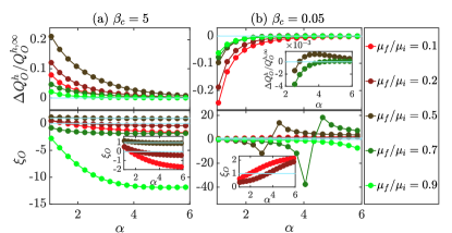
Figure 6: Column (a): $\Delta Q_{O}^{h}/Q_{O}^{h,\infty}$ (upper panel) and $\xi_{O}$ (bottom panel and zoomed-in inset) as a function of $\alpha$ for different values of $\mu_{f}/\mu_{i}$ at $\beta_{c}=5$. Column (b): The same as in column (a) applied to the high-temperature case with $\beta_{c}=0.05$. The solid horizontal lines in the upper panels and associated inset indicate $\Delta Q_{O}^{h}=0$. The horizontal lines in the bottom panels and associated insets indicate $\xi_{O}=1$ and $\xi_{O}=0$. The remaining parameters are: $\hbar=k_{B}=1$, $\mu_{i}=2$, $J=\Delta=1$, $\beta_{h}/\beta_{c}=0.2$, and $L=2000$. All quantities are dimensionless.

According to the first law of thermodynamics, the net work extracted by the quantum Stirling cycle is

$$W_{S} =Q_{\mathrm{I}}+Q_{\mathrm{II}}+Q_{\mathrm{III}}+Q_{\mathrm{IV}}$$

$$=\sum_{k>0}\left\{\frac{2}{\beta_{h}}\left[\ln\cosh\left(\frac{\beta_{h}\varepsilon_{k}^{f}}{2}\right)-\ln\cosh\left(\frac{\beta_{h}\varepsilon_{k}^{i}}{2}\right)\right]\right.$$

$$+\left.\frac{2}{\beta_{c}}\left[\ln\cosh\left(\frac{\beta_{c}\varepsilon_{k}^{i}}{2}\right)-\ln\cosh\left(\frac{\beta_{c}\varepsilon_{k}^{f}}{2}\right)\right]\right\}.$$ (20)

For each cycle, the amount of heat $Q_{S}^{h}$ absorbed by the working medium reads

$$Q_{S}^{h} =Q_{\mathrm{I}}+Q_{\mathrm{IV}}$$

$$=\sum_{k>0}\left\{\frac{2}{\beta_{h}}\left[\ln\cosh\left(\frac{\beta_{h}\varepsilon_{k}^{f}}{2}\right)-\ln\cosh\left(\frac{\beta_{h}\varepsilon_{k}^{i}}{2}\right)\right]\right.$$

$$+\left.\left[\varepsilon_{k}^{i}\tanh\left(\frac{\beta_{c}\varepsilon_{k}^{i}}{2}\right)-\varepsilon_{k}^{f}\tanh\left(\frac{\beta_{h}\varepsilon_{k}^{f}}{2}\right)\right]\right\}.$$ (21)

Therefore the efficiency of the heat engine reads

$$\eta_{S}=\frac{W_{S}}{Q_{S}^{h}}.$$ (22)

We stress that in order to extract work from the engine we should have $W_{S}>0$, as in the Otto cycle, and the efficiency $\eta_{S}$ is also limited by the Carnot efficiency $\eta_{c}$ Ma et al. (2017).

Based on the above results, in the next section we investigate the effects of the long-range interactions on the performance of a quantum heat engine which drives through the quantum Otto and Stirling cycles, respectively.

IV Results and discussions

In our numerical calculation, the chemical potential varies from the initial value $\mu_{i}=2$ to the final value $\mu_{f}$ with $0\leq\mu_{f}\leq 2$. To unveil the influences of the long-range interactions on the performance of the quantum engine, for both Otto and Stirling cycles we consider the following ratios:

$$\mathcal{R}^{\kappa}_{W}=\frac{W_{\kappa}}{W_{\kappa}^{\infty}},\ \mathcal{R}^{\kappa}_{\eta}=\frac{\eta_{\kappa}}{\eta_{\kappa}^{\infty}},$$ (23)

where $\kappa=O$ ($S$) corresponds to the Otto (Stirling) cycle, $W_{\kappa}$ ($\eta_{\kappa}$) is the work output (efficiency) with finite $\alpha$, while $W_{\kappa}^{\infty}$ ($\eta_{\kappa}^{\infty}$) represents its short-range (with $\alpha=\infty$) counterpart.

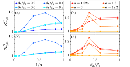
Figure 7: Left column: The maximum work output ratio $\mathcal{R}_{W,\mathrm{m}}^{O}$ (a) and the maximum efficiency ratio $\mathcal{R}_{\eta,\mathrm{m}}^{O}$ (c) of Otto cycle as a function of $\alpha$, with different curves in each panel representing different ratios of bath temperatures. Right column: $\mathcal{R}_{W,\mathrm{m}}^{O}$ (b) and $\mathcal{R}_{\eta,\mathrm{m}}^{O}$ (d) as a function of $\beta_{h}/\beta_{c}$ for different $\alpha$ (different colors). Parameters are $\hbar=k_{B}=1$, $\beta_{c}=5$, $J=\Delta=1$, and $L=2000$.

The ratios defined in Eq. (23) compare the net work output and efficiency of a long-range interacting heat engine with that of a short-range interacting heat engine. If $\mathcal{R}_{W}^{\kappa}=1$ and $\mathcal{R}_{\eta}^{\kappa}=1$, the long-range interacting heat engine has the same performance as its short-range counterpart. Conversely, having $\mathcal{R}_{W}^{\kappa}>1,\mathcal{R}_{\eta}^{\kappa}>1$ indicates that there is an enhancement in engine performance induced by the long-range interactions. Finally, $\mathcal{R}_{W}^{\kappa}<1,\mathcal{R}_{\eta}^{\kappa}<1$ mean that the quantum heat engine with short-range interacting working medium is more beneficial. In our following study, we will investigate the dependence of these ratios on the interacting range $\alpha$ for the Otto and Stirling cycles, respectively.

We separately consider the cases in which the quantum engine operating at low and high temperature with the ratio of bath inverse temperature $\beta_{h}/\beta_{c}$ is fixed. For the low-temperature case, we take the inverse temperature of the cold bath as $\beta_{c}=5$, while for the high-temperature case we chose $\beta_{c}=0.05$. As we have pointed out in Sec. II, we focus on the situation $\alpha>1$, where a transition between the long and short ranges occurs.

Before we present our results for a specific thermodynamic cycle, we first illustrate the notable differences in the behavior of quasiparticle energy $\varepsilon_{k}$ [cf. Eq. (7)] arising from the long-range interactions. Figure 4 depicts the quasiparticle energy as a function of momentum $k$ and $\mu_{f}$ for different $\alpha$. By comparing with the short-range interactions case [panel (d)], one can see that the long-range interactions have strong impacts on the behavior of quasiparticle energy. As the work output and efficiency of a heat engine involve the sum of quasiparticle energy, the differences in the quasiparticle energy from the interacting range allow us to expect that long-range interactions should affect the performance of the quantum engine.

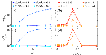
Figure 8: Same as Fig. 7 but for the high-temperature case with $\beta_{c}=0.05$.

IV.1 Results for quantum Otto cycle

By using the results outlined in Sec. III.1, we are able to calculate the work output $W_{O}$ and efficiency $\eta_{O}$ of the Otto cycle for different interacting ranges and cycle parameters. We first focus on the behavior of work output ratio $\mathcal{R}_{W}^{O}$ for several ranges of interactions.

In the first row of Fig. 5, we plot $\mathcal{R}_{W}^{O}$ as a function of $\mu_{f}/\mu_{i}$ for different values of $\alpha$ at $\beta_{c}=5$ [panel (a)] and $\beta_{c}=0.05$ [panel (b)]. We first notice that for some chemical potential regimes the value of $\mathcal{R}_{W}^{O}$ can be greater than $1$ and increases with decreasing $\alpha$. This means that the long-range interactions in the Kitaev chain can enhance the performance of the Otto engine. Specifically, for the engine operating at low temperature with $\beta_{c}=5$, the work output will get a significant enhancement with increasing (decreasing) the range of interactions ($\alpha$) when $\mu_{f}/\mu_{i}>0.5$, as shown in Fig. 5(a). On the contrary, the work output is enhanced by the long-range interactions in the region $\mu_{f}/\mu_{i}<0.5$ for the high temperature case with $\beta_{c}=0.05$, as evidenced by Fig. 5(b).

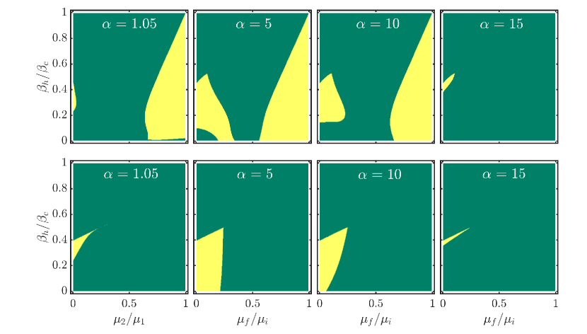
Figure 9: Enhancement regions of the Otto cycle in parameter space for different values of $\alpha$. Here the enhancement regions are identified as the regions with $\mathcal{R}_{W}^{O}>1$ and $\mathcal{R}_{\eta}^{O}>1$. The yellow regions indicate the enhancement regions in parameter space under which the performance of the heat engine is enhanced by long-range interactions. The upper panels are the results for the low-temperature case with $\beta_{c}=5$, and the bottom panels represent the high-temperature case with $\beta_{c}=0.05$. The remaining parameters are $\hbar=k_{B}=1$, $\mu_{i}=2$, $J=\Delta=1$, and $L=2000$.

We further see that $\mathcal{R}_{W}^{O}$ is minimized at around $\mu_{f}/\mu_{i}=0.5$, which corresponds to the critical point of the system. In particular, for the case of low temperature, $\mathcal{R}_{W}^{O}$ shows a remarkable decrease at long-range interactions. It is known that the work output takes its local minimal value at the critical point of the system Fadaie et al. (2018). The dramatic drop in $\mathcal{R}_{W}^{O}$ near $\mu_{f}/\mu_{i}=0.5$ implies that the negative impact of the phase transition on the extractable work can be enhanced by long-range interactions.

The efficiency ratio $\mathcal{R}_{\eta}^{O}$ for different ranges of interactions at low and high temperature cases are displayed in the second row of Fig. 5. As shown in Fig. 5(c), at low temperature with $\beta_{c}=5$, the efficiency for a long-range interacting engine is always superior to its short-range counterpart as long as $\mu_{f}/\mu_{i}\neq 0.5$. Around the critical point $\mu_{f}/\mu_{i}=0.5$, $\mathcal{R}_{\eta}^{O}$ also has a significant decrease for long-range interactions, indicating the enhanced negative impact on the efficiency at the critical point.

For the case of high temperature with $\beta_{c}=0.05$, as can be seen from Fig. 5(d), the enhancement in efficiency due to the long-range interactions occurs only for smaller $\mu_{f}/\mu_{i}$ when $\alpha\geq 1.2$. For $1<\alpha<1.2$, the long-range interactions show a universal negative impact on the efficiency of the engine. Moreover, we still see $\mathcal{R}_{\eta}^{O}$ is minimized around the critical point in the case of high temperature. We stress that the efficiency is always less than Carnot efficiency, regardless of interacting ranges and bath temperatures.

The features observed for $\mathcal{R}_{W}^{O}$ and $\mathcal{R}_{\eta}^{O}$ can be understood as follows. We first rewrite $\mathcal{R}_{W}^{O}$ and $\mathcal{R}_{\eta}^{O}$ as

$$\mathcal{R}_{W}^{O}=1-\xi_{O}\frac{\Delta Q_{O}^{h}}{Q_{O}^{h,\infty}},$$

$$\mathcal{R}_{\eta}^{O}=1-\frac{\Delta Q_{O}^{h}}{Q_{O}^{h,\infty}}\frac{\xi_{O}-1}{1-\Delta Q_{O}^{h}/Q_{O}^{h,\infty}},$$ (24)

where $\Delta Q_{O}^{h}=Q_{O}^{h,\infty}-Q_{O}^{h}$ is the absorbed heat differences between short- and long-range engines, and $\xi_{O}=\Delta W_{O}/(\eta_{O}^{\infty}\Delta Q_{O}^{h})$ with $\Delta W_{O}=W_{O}^{\infty}-W_{O}$. We thus show that the $\Delta Q_{O}^{h}/Q_{O}^{h,\infty}$ and $\xi_{O}$ act as the indicators of enhancement in engine performance. Figure 6 displays $\Delta Q_{O}^{h}/Q_{O}^{h,\infty}$ and $\xi_{O}$ versus $\alpha$ for several representative values of $\mu_{f}/\mu_{i}$ with $\beta_{c}=5$ [column (a)] and $\beta_{c}=0.05$ [column (b)].

At low temperature [column (a) in Fig. 6], as can be seen from the upper panel, $\Delta Q_{O}^{h}/Q_{O}^{h,\infty}$ is always greater than zero and decreases with increase in $\alpha$, irrespective of the value of $\mu_{f}/\mu_{i}$. On the other hand, for all ranges of interactions studied, the values of $\xi_{O}$ are less than zero in the region $\mu_{f}/\mu_{i}>0.5$. According to Eq. (IV.1), this makes both $\mathcal{R}_{W}^{O}$ and $\mathcal{R}_{\eta}^{O}$ greater than $1$ for $\mu_{f}/\mu_{i}>0.5$. For the case of $\mu_{f}/\mu_{i}<0.5$, we notice that $0<\xi_{O}<1$ when $\alpha<2$, while as $\alpha>2$, the value of $\xi_{O}$ becomes less than zero (see the inset in the bottom panel). This indicates that in the region $\mu_{f}/\mu_{i}<0.5$, $\mathcal{R}_{W}^{O}<1$ for the system with long-range interactions and increases with decreasing the range of interactions. However, as $\xi_{O}<1$ holds for any value of $\alpha$, $\mathcal{R}_{\eta}^{O}$ will always be greater than $1$ at $\mu_{f}/\mu_{i}<0.5$. At the critical point $\mu_{f}/\mu_{i}=0.5$, we find that $\Delta Q_{O}^{h}/Q_{O}^{h,\infty}$ is maximized, regardless of the values of $\alpha$. Meanwhile, the behavior of $\xi_{O}$ shows that $\xi_{O}>1$ at smaller $\alpha$ and it approximately equal to $1$ for $\alpha>2$. These two factors give rise to the remarkable decrease in $\mathcal{R}_{W}^{O}$ and $\mathcal{R}_{\eta}^{O}$ at $\mu_{f}/\mu_{i}=0.5$.

In column (b) of Fig. 6 we demonstrate the same analysis for the case of high temperature. For all the ranges of interactions studied, $\Delta Q_{O}^{h}/Q_{O}^{h,\infty}<0$ and $\xi_{O}>0$ at $\mu_{f}/\mu_{i}<0.5$. This leads to $\mathcal{R}_{W}^{O}>1$ for small values of the ratio $\mu_{f}/\mu_{i}$. In addition, as shown in the inset of the bottom panel, for $\mu_{f}/\mu_{i}<0.5$, at smaller $\alpha$ we have $\xi_{O}<1$, but for greater values of $\alpha$, we have $\xi_{O}>1$. This means that the efficiency ratio changes from $\mathcal{R}_{\eta}^{O}<1$ for long-range interactions to $\mathcal{R}_{\eta}^{O}>1$ as the range of interactions decreases in the region $\mu_{f}/\mu_{i}<0.5$. However, when $\mu_{f}/\mu_{i}\geq 0.5$, we see that regardless of the range of interactions, the second term $\xi_{O}\Delta Q_{O}^{h}/Q_{O}^{h,\infty}$ in $\mathcal{R}_{W}^{O}$ [cf. Eq. (IV.1)] is always greater than zero, despite that $\Delta Q_{O}^{h}/Q_{O}^{h,\infty}$ can vary from negative values to positive values (see the inset in the upper panel). As a consequence, the value of $\mathcal{R}_{W}^{O}$ is less than $1$ for greater values of $\mu_{f}/\mu_{i}$. Moreover, as $\Delta Q_{O}^{h}/Q_{O}^{h,\infty}<0(>0)$ is associated with $\xi_{O}<0(>1)$ at $\mu_{f}/\mu_{i}\geq 0.5$, the value of $\mathcal{R}_{\eta}^{O}$ is also less than $1$. Finally, in the high-temperature case, the maximal value of $|\Delta Q_{O}^{h}/Q_{O}^{h,\infty}|$ is still reached at the critical point, indicating $\mathcal{R}_{W}^{O}$ and $\mathcal{R}_{\eta}^{O}$ have a significant decrease at $\mu_{f}/\mu_{i}=0.5$.

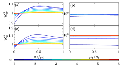
Figure 10: Work output ratio $\mathcal{R}_{W}^{S}$ of the Stirling cycle as a function of $\mu_{f}/\mu_{i}$ with $\beta_{c}=5$ (a) and $\beta_{c}=0.05$ (b) and the efficiency ratio $\mathcal{R}_{\eta}^{S}$ as a function of $\mu_{f}/\mu_{i}$ with $\beta_{c}=5$ (c) and $\beta_{c}=0.05$ (d) for $\alpha\in[1.05,6]$. The remaining parameters are $\hbar=k_{B}=1$, $\mu_{i}=2$, $\beta_{h}/\beta_{c}=0.2$, $J=\Delta=1$, and $L=2000$.

To gain further insight into the details of the long-range interaction impacts on the performance of the quantum engine, we plot $\mathcal{R}_{W,\mathrm{m}}^{O}$ and $\mathcal{R}_{\eta,\mathrm{m}}^{O}$, defined as the maximum in $\mathcal{R}_{W}^{O}$ and $\mathcal{R}_{\eta}^{O}$, versus $\alpha$ for different values of $\beta_{h}/\beta_{c}$ with $\beta_{c}=5$ in the left column of Fig. 7. On can immediately see a striking similarity between $\mathcal{R}_{W,\mathrm{m}}^{O}$ and $\mathcal{R}_{\eta,\mathrm{m}}^{O}$. Regardless of the value of $\beta_{h}/\beta_{c}$, both of them converge towards unity in the short-range limit $\alpha\to\infty$, as expected. However, at $\beta_{h}/\beta_{c}=0.4$, we see that $\mathcal{R}_{W,\mathrm{m}}^{O}$ and $\mathcal{R}_{\eta,\mathrm{m}}^{O}$ exhibit a remarkably different behavior as compared to the results obtained for other values of $\beta_{h}/\beta_{c}$. Specifically, at $\beta_{h}/\beta_{c}=0.4$, both $\mathcal{R}_{W,\mathrm{m}}^{O}$ and $\mathcal{R}_{\eta,\mathrm{m}}^{O}$ first experience a growth and then decrease to unity as $\alpha$ increases, whereas we observe a monotonous decrement in $\mathcal{R}_{W,\mathrm{m}}^{O}$ and $\mathcal{R}_{\eta,\mathrm{m}}^{O}$ with increase in $\alpha$ for $\beta_{h}/\beta_{c}\neq 0.4$. Moreover, the observed $\beta_{h}/\beta_{c}$ dependence in the behaviors of $\mathcal{R}_{W,\mathrm{m}}^{O}$ and $\mathcal{R}_{\eta,\mathrm{m}}^{O}$ imply that the bath temperatures can strongly influence the enhancing ability of long-range interactions. In the right column of Fig. 7, we show $\beta_{h}/\beta_{c}$ dependence of $\mathcal{R}_{W,\mathrm{m}}^{O}$ and $\mathcal{R}_{\eta,\mathrm{m}}^{O}$ for several values of $\alpha$. We see again the remarkable resemblance between $\mathcal{R}_{W,\mathrm{m}}^{O}$ and $\mathcal{R}_{\eta,\mathrm{m}}^{O}$ when $\alpha>1.025$. At $\alpha=1.025$, we can see that $\mathcal{R}_{W,\mathrm{m}}^{O}$ increases monotonously as $\beta_{h}/\beta_{c}$ increases, while $\mathcal{R}_{\eta,\mathrm{m}}^{O}$ shows a growth followed by a decrement with increase in $\beta_{h}/\beta_{c}$. The features in Fig. 7 indicate that for an Otto cycle operating at low temperature, there exists an optimal condition for which the maximum enhancement in the work output and efficiency induced by long-range interactions are reached at the same time. For the case considered here, it is approximately given by $\alpha\approx 1.5$, $\beta_{h}/\beta_{c}\approx 0.4$.

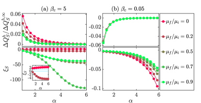
Figure 11: Column (a): $\Delta Q_{S}^{h}/Q_{S}^{h,\infty}$ (upper panel) and $\xi_{S}$ (bottom panel and zoomed-in inset) as a function of $\alpha$ for different values of $\mu_{f}/\mu_{i}$ at $\beta_{c}=5$. The solid horizontal lines in the inset indicate $\xi_{S}=0$ and $\xi_{S}=1$, respectively. Column (b): The same as in column (a) applied to the high-temperature case with $\beta_{c}=0.05$. The remaining parameters are $\hbar=k_{B}=1$, $\mu_{i}=2$, $\beta_{h}/\beta_{c}=0.2$, $J=\Delta=1$, and $L=2000$. All quantities are unitless.

For the high temperature case, the $\alpha$ and $\beta_{h}/\beta_{c}$ dependencies of $\mathcal{R}_{W,\mathrm{m}}^{O}$ and $\mathcal{R}_{\eta,\mathrm{m}}^{O}$ are shown in Fig. 8. As can be seen from the left column of Fig. 8, the behavior of $\mathcal{R}_{W,\mathrm{m}}^{O}$ is qualitatively similar to $\mathcal{R}_{\eta,\mathrm{m}}^{O}$. Namely, both of them are decreased with an increase in $\alpha$ and approaching unity as $\alpha\to\infty$, irrespective of the value of $\beta_{h}/\beta_{c}$. On the other hand, for different values of $\alpha$, the observed $\beta_{h}/\beta_{c}$ dependence of $\mathcal{R}_{W,\mathrm{m}}^{O}$ is also very similar to $\mathcal{R}_{\eta,\mathrm{m}}^{O}$, as evidenced by the right column in Fig. 8. The results in Fig. 8 further verify that the above-defined optimal condition also existed in the case of high temperature. The optimal condition for the case studied here is given by $\alpha=1.025$, $\beta_{h}/\beta_{c}=0.4$, different from the case of low temperature. By comparing Figs. 7 and 8, we further notice that there is a greater enhancement in engine performance at the high temperature.

It is also of interest to study how the regions of enhancement in parameter space evolve as the range of interactions is changed from the long-rang to short-range limit. In Fig. 9 we plot the regions where the enhancement is absent (dark green) or present (yellow) for several values of $\alpha$ with $\beta_{c}=5$ (upper row) and $\beta_{c}=0.05$ (bottom row). Here, in our study, the enhancement regions are the regions with $\mathcal{R}_{W}^{O}>1$ and $\mathcal{R}_{\eta}^{O}>1$. We see that for both the low- and high-temperature cases, the enhancement regions first undergo an expansion in parameter space and then shrink with increasing $\alpha$. One can expect that such regions will vanish as $\alpha\to\infty$. Here, it is worth mentioning that $\mathcal{R}_{W}^{O}$ and $\mathcal{R}_{\eta}^{O}$ decrease with increasing $\alpha$ and approach $1$ as $\alpha\to\infty$. The expansion of the enhancement regions is, therefore, associated with the reduction in the enhancing ability of the long-range interactions. We finally note that the size of the enhancement regions in the case of low temperature is always lager than the corresponding high-temperature case.

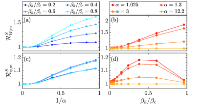
Figure 12: Left column: The maximum work output ratio $\mathcal{R}_{W,\mathrm{m}}^{S}$ (a) and the maximum efficiency ratio $\mathcal{R}_{\eta,\mathrm{m}}^{S}$ (c) of the Stirling cycle as a function of $\alpha$ for different values of $\beta_{h}/\beta_{c}$. Right column: $\mathcal{R}_{W,\mathrm{m}}^{S}$ (b) and $\mathcal{R}_{\eta,\mathrm{m}}^{S}$ (d) as a function of $\beta_{h}/\beta_{c}$ for several $\alpha$. The remaining parameters are $\hbar=k_{B}=1$, $\beta_{c}=5$, $J=\Delta=1$, and $L=2000$.

IV.2 Results for quantum Stirling cycle

We continue our study by exploring the long-range interaction effects on the performance of the quantum Stirling cycle. According to the results in Sec. III.2, we have calculated the work output ratio $\mathcal{R}_{W}^{S}$ and efficiency ratio $\mathcal{R}_{\eta}^{S}$ defined in Eq. (23) for a Stirling cycle with different ranges of interactions and cycle parameters; the results are shown in Fig. 10.

First, for the case of low temperature with $\beta_{c}=5$, both the work output and efficiency of the Stirling cycle are enhanced by the long-range interactions at greater $\mu_{f}/\mu_{i}$; see panels (a) and (c) in Fig. 10. Moreover, different from the results in the Otto cycle, we see that the maximal values of $\mathcal{R}_{W}^{S}$ and $\mathcal{R}_{\eta}^{S}$ are obtained near the critical point $\mu_{f}/\mu_{i}=0.5$, and increase with decreasing $\alpha$. Hence, for the Stirling cycle, the enhancement effect of long-range interactions can be boosted by the critical point. On the contrary, at high temperature with $\beta_{c}=0.05$, as can be seen from panels (b) and (d) in Fig. 10, we have $\mathcal{R}_{W}^{S}<1$ and $\mathcal{R}_{\eta}^{S}<1$ over the whole parameter region. Therefore, the long-range interactions are useless to improve the performance of the Stirling cycle if it is operating at high temperature.

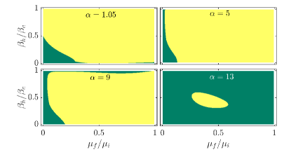
Figure 13: Regions of enhancement in the parameter space of a Stirling cycle for different values of $\alpha$. The enhancement regions are defined as the regions with $\mathcal{R}_{W}^{S}>1$ and $\mathcal{R}_{\eta}^{S}>1$. Yellow and dark green shaded domains indicate the regions with enhancement and no enhancement. The parameters are: $\hbar=k_{B}=1$, $\mu_{i}=2$, $\beta_{c}=5$, $\beta_{h}/\beta_{c}=0.2$, $J=\Delta=1$, and $L=2000$.

To understand the features observed in Fig. 10, as we have done for the case of the Otto cycle, we recast $\mathcal{R}_{W}^{S}$ and $\mathcal{R}_{\eta}^{S}$ as follows:

$$\mathcal{R}_{W}^{S}=1-\xi_{S}\frac{\Delta Q_{S}^{h}}{Q_{S}^{h,\infty}},$$

$$\mathcal{R}_{\eta}^{S}=1-\frac{\Delta Q_{S}^{h}}{Q_{S}^{h,\infty}}\frac{\xi_{S}-1}{1-\Delta Q_{S}^{h}/Q_{S}^{h,\infty}},$$ (25)

where $\Delta Q_{S}^{h}=Q_{S}^{h,\infty}-Q_{S}^{h}$ is the absorbed heat difference of the Stirling cycle, and $\xi_{S}=\Delta W_{S}/(\eta_{S}^{\infty}\Delta Q_{S}^{h})$ with $\Delta W_{S}=W_{S}^{\infty}-W_{S}$. Then, we consider the dependences of $\Delta Q_{S}^{h}/Q_{S}^{h,\infty}$ and $\xi_{S}$ on the range of interactions for different values of $\mu_{f}/\mu_{i}$. Column (a) of Fig. 11 shows $\Delta Q_{S}^{h}/Q_{S}^{h,\infty}$ (upper panel) and $\xi_{S}$ (bottom panel) versus $\alpha$ for a few representative values of $\mu_{f}/\mu_{i}$ at low temperature. Clearly, we always have $\Delta Q_{S}^{h}/Q_{S}^{h,\infty}>0$ for all ranges of interactions and values of $\mu_{f}/\mu_{i}$. Therefore there are negative values of $\xi_{S}$ at $\mu_{f}/\mu_{i}\geq 0.2$ (see the bottom panel), indicating $\mathcal{R}_{S}^{W}>1$ and $\mathcal{R}_{\eta}^{S}>1$. For the case of $\mu_{f}/\mu_{i}=0$, as can be seen from the inset in the bottom panel, we always have $\xi_{S}>1$, resulting in $\mathcal{R}_{W}^{S}<1$ and $\mathcal{R}_{\eta}^{S}<1$. In marked contrast to the low-temperature case, at high temperature with $\beta_{c}=0.05$ we find that $\Delta Q_{S}^{h}/Q_{S}^{h,\infty}<0$ and $\xi_{S}<0$, regardless of the values of $\alpha$ and $\mu_{f}/\mu_{i}$, as shown in column (b) of Fig. 11. We thus have $\mathcal{R}_{W}^{S}<1$ and $\mathcal{R}_{\eta}^{S}<1$, independent of $\alpha$ and $\mu_{f}/\mu_{i}$.

As we focus on the enhancement effect of the long-range interactions, we only consider the low-temperature case in the following studies of the Stirling cycle. Figure 12 depicts the maximum work output ratio $\mathcal{R}_{W,\mathrm{m}}^{S}$ and the maximum efficiency ratio $\mathcal{R}_{\eta,\mathrm{m}}^{S}$ in the Stirling cycle. We see that as $\alpha$ increases, $\mathcal{R}_{W,\mathrm{m}}^{S}$ and $\mathcal{R}^{S}_{\eta,\mathrm{m}}$ converge towards $1$ in a similar way; see panels (a) and (c) in Fig. 12. However, the dependence of $\mathcal{R}_{W,\mathrm{m}}^{S}$ on $\beta_{h}/\beta_{c}$ is prominent, different from the case of maximum efficiency ratio, as visible in panels (b) and (d) of Fig. 12. Specifically, $\mathcal{R}_{W,\mathrm{m}}^{S}$ increases monotonously with an increase in $\beta_{h}/\beta_{c}$, while the increment in $\mathcal{R}_{\eta,\mathrm{m}}^{S}$ at smaller $\beta_{h}/\beta_{c}$ is followed by a decrement at greater $\beta_{h}/\beta_{c}$. As a consequence, the optimal condition extracted from $\mathcal{R}_{W,\mathrm{m}}^{S}$ in Figs. 12(a) and 12(b) is inconsistent with that obtained from the results of $\mathcal{R}_{\eta,\mathrm{m}}^{S}$ [see Figs. 12(c) and 12(b)]. This disagreement means that the maximum enhancement in work output and efficiency cannot be achieved simultaneously by the long-range interactions in the Stirling cycle. This is in sharp contrast to the Otto cycle, where the work output ratio and efficiency ratio can be maximized under the same condition.

We finally investigate the evolution of enhancement regions in the parameter space of the Stirling cycle with decreasing the range of interactions. As in the Otto cycle, the enhancement regions in the Stirling cycle are still identified as the regions with $\mathcal{R}_{W}^{S}>1$ and $\mathcal{R}_{\eta}^{S}>1$. Figure 13 shows the enhancement regions of the Stirling cycle for several values of $\alpha$. We see that as $\alpha$ increases, the enhancement regions first experience an expansion and then shrink in the parameter space, similar to the case of the Otto cycle. As expected, the enhancement regions will disappear in the short-range limit $\alpha\to\infty$. Moreover, such as in the Otto cycle, due to the values of $\mathcal{R}_{W}^{S}$ and $\mathcal{R}_{\eta}^{S}$ decreasing with increasing $\alpha$, the expansion of the enhancement regions will associate with a larger reduction in the enhancing ability of the long-range interactions.

V Conclusions

In conclusion, we have examined how the long-range interactions in quantum many-body systems affect the performance of quantum heat engines. To this end, we have introduced a many-body quantum heat engine with a long-range Kitaev chain as its working medium. The integrability nature of the long-range interacting Kitaev chain allows us to study the performance of the heat engine through fully analytical results. We have demonstrated that the long-range interactions exhibit remarkable and nontrivial impacts on the performance of the quantum heat engine. We have considered quantum heat engine operators with different thermodynamic cycles–the Otto cycle and the Stirling cycle.

For the Otto cycle operating at low temperature, we found that in all studied figures of merit of engine performance, including net work output and efficiency, the long-range interactions enhance the engine performance for certain cycle parameter regimes. This enhancement effect still persists when the engine is working at high temperature. However, near the critical point of the system, the work output and efficiency decrease dramatically with increasing the range of interactions, irrespective of the bath temperatures. In the case of a Stirling cycle at low temperature, the long-range interactions exhibit a similar enhancement effect on the performance of the engine. However, different from the Otto cycle, in this case the long-range interactions lead to a maximum enhancement of the performance of the Stirling cycle around the critical point of the system. We found the universal negative impact of the long-range interactions when the Stirling cycle operated at high temperature.

For both cycles we investigated the possibility of long-range interactions leading to a maximum enhancement in work output and efficiency of the quantum heat engine at the same time. We found that in the Otto cycle the maximum enhancement in the performance of the engine can be achieved simultaneously by the long-range interactions, while this is not true in the case of the Stirling cycle. In addition, we also explored the dependencies of the enhancement regions in the cycle parameter space on the range of interactions and showed that with a decrease in range of interactions the enhancement regions first expand and then quickly shrink. Such regions finally vanish as $\alpha\to\infty$.

Our results evidence that the long-range interactions in many-body systems have strong effects on the performance of quantum heat engines. Therefore, our work provides an additional insight into how to improve engine performance in quantum many-body heat engines Jaramillo et al. (2016); Beau et al. (2016); Li et al. (2018); Chen et al. (2019); Yunger Halpern et al. (2019); Kloc et al. (2019); Hartmann et al. (2019); S. et al. (2020). Moreover, the experimental realization of one-dimensional long-range Kitaev chains in physical systems has been proposed in many studies Tong et al. (2013); Benito et al. (2014); Pientka et al. (2013, 2014); Giuliano et al. (2018). In particular, by using an experimental platform based on a superconductor in proximity to a two-dimensional electron gas with strong spin-orbit coupling Hell et al. (2017); Pientka et al. (2017), a very recent work has been demonstrated that long-range Kitaev chains can be obtained via planar Josephson junctions Liu et al. (2018). In this scheme, tuning of the range of interactions can be achieved by controlling the strength of the Zeeman field, whereas the tunable chemical potential is accomplished through the phase difference between two $s$-wave superconductors. On the other hand, several proposals for realizing quantum heat engines in superconducting devices have been discussed in a variety of works Campisi et al. (2015); Marchegiani et al. (2016). These facts lead us to believe that our results could be experimentally verified.

We expect the performance enhancement of quantum engines by long-range interactions still holds in other long-range interacting systems, such as long-range interacting spin systems. It will be interesting to systematically study how the range of interactions affect the engine performance in different long-range interacting systems. Another interesting extension of the present work is to analyze the role of the range of interactions in finite time cycles. By considering that long-range interacting spin systems have been realized in recent experiments Jurcevic et al. (2014); Richerme et al. (2014), we hope that our present results would be able to trigger more experimental efforts to investigate the effects of long-range interactions on the performance of quantum heat engines.