NLTE for APOGEE: Simultaneous Multi-Element NLTE Radiative Transfer.

Abstract

Context. Relaxing the assumption of Local Thermodynamic Equilibrium (LTE) in modelling stellar spectra is a necessary step to determine chemical abundances better than about 10 % in late-type stars.

Aims. In this paper we describe our efforts gearing up to perform multi-element (Na, Mg, K, and Ca) Non-LTE (NLTE) calculations that can be applied to the APOGEE survey.

Methods. The new version of TLUSTY  allows for the calculation of restricted NLTE in cool stars using pre-calculated opacity tables. We demonstrate that TLUSTY gives consistent results with MULTI, a well-tested code for NLTE in cool stars. We use TLUSTY to perform LTE and a series of NLTE calculations using all combinations of 1, 2, 3 and the 4 elements mentioned above simultaneously in NLTE.

Results. In this work we take into account how departures from LTE in one element can affect others through changes in the opacities of Na, Mg, K, and Ca. We find that atomic Mg, which provides strong UV opacity, and exhibits significant departures from LTE in the low-energy states, can impact the NLTE populations of Ca, leading to abundance corrections as large as 0.07 dex. The differences in the derived abundances between the single-element and the multi-element cases can exceed those between the single-element NLTE determinations and an LTE analysis, warning that this is not always a second-order effect. By means of detailed tests for three stars with reliable atmospheric parameters (Arcturus, Procyon and the Sun) we conclude that our NLTE calculations provide abundance corrections that can amount in the optical up to 0.1, 0.2 and 0.7 dex for Ca, Na and K, but LTE is a good approximation for Mg. In the H-band, NLTE corrections are much smaller, and always under to 0.1 dex. The derived NLTE abundances in the optical and in the IR are consistent. For all four elements, in all three stars, NLTE line profiles fit better the observations than the LTE counterparts.

Conclusions. The atomic elements in ionisation stages where over-ionisation is an important NLTE mechanism are likely affected by departures from LTE in Mg . Special care must be taken with the collisions adopted for high-lying levels when calculating NLTE profiles of lines in the H-band. The derived NLTE corrections in the optical and in the H-band differ, but the derived NLTE abundances are consistent between the two spectral regions.

1 Introduction

The determination of chemical abundances in stars relies on the comparison with physical models of stellar atmospheres involving a number of approximations. Among these, the assumption that the gas is in local thermodynamic equilibrium (LTE), i.e. finding the atomic populations using the Saha and Boltzmann equations from the local temperature and electron density, is known to be one, if not the main, factor limiting the determination of accurate abundances. One of the difficulties in relaxing the LTE assumption, performing Non-LTE (NLTE) calculations, is the need for detailed data on the radiative and collisional processes that affect the atoms of interest. Over the last decade, much progress has been made in this direction, and a substantial effort investment has been made to implement NLTE in the analysis of stellar spectra (Allende Prieto, 2016; Asplund, 2005).

Implementing NLTE is particularly hard for very large spectroscopic samples with high-resolution and wide spectral coverage, since it requires collecting all the necessary data for many ions and performing time-consuming calculations. Surveys such as GALAH have started to provide NLTE abundances for a few elements (Buder et al., 2018), and we are gearing up to do the same for APOGEE (Majewski et al., 2017). In this paper we address the important question of whether NLTE calculations can be performed for a chemical element at a time, or NLTE effects from one element affect others significantly.

In contrast to NLTE radiative transfer calculations for hot stars, where H and other other elements must be considered in NLTE in order to obtain reliable atmospheric structure and spectrum (Auer & Mihalas, 1969a, b, 1970), NLTE radiative transfer calculations in cool stars are performed using the trace element approach, where the effects of the NLTE populations on the atmospheric structure and background opacities are neglected. The justification for this approach lies in the argument that the abundance of the element under study, and the differences between the LTE and NLTE populations, are small enough that they do not affect other elements or the stellar atmospheric structure.

In the calculations described in this paper we do not allow the atmospheric structure to change, i.e., the temperature, electron and density distributions are kept fixed. In this case interactions between the NLTE populations for different elements in our calculations take place trough the opacity. In the specific case of Mg and Ca, the broad resonance lines of their first ions provide an important contribution to the opacities between $\sim$2 700 and 4 000 Å in solar-type stars, and NLTE populations of the excited levels of those ions can also affect the opacity ”seen” by other elements, and thus modify their NLTE populations. Elements with small contributions to the opacity will then have a negligible impact on other elements calculated simultaneously in NLTE.

Section 2 describes the model atoms and the reference observations we will be testing our models against. Section 3 provides an overview of the basics of our NLTE calculations. Section 4 compares calculations for a single element with two different NLTE codes: MULTI and TLUSTY. Section 5 describes our multi-element calculations and in Section 6 we confront them with observations. We focus on the most relevant results for the APOGEE survey in Section 7, and give our conclusions in section 8.

2 Model atoms and reference stars

For this work, we used 4 different atomic elements: Na i, Mg i & ii, K i and Ca i & ii. The atomic data were drawn from different sources. The Mg  and Ca  model atoms were basically the same as in Osorio et al. (2015, 2019) respectively. while the model atoms for Na  and K  were created from scratch for this work. Three reference stars with observational data of exceptional quality and well-determined stellar parameters were adopted: Procyon, the Sun and Arcturus, The observational data and the synthetic model atmospheres were the same as in Osorio et al. (2019). A description of these data will be given in § 2.4.

2.1 Mg and Ca

Energy levels were taken mostly from the NIST database (Ralchenko et al., 2014), line data were taken from VALD (Kupka et al., 2000; Ryabchikova et al., 2015) , NIST, and in the case of Ca i, from Yu & Derevianko (2018). Continuum data were taken from the TOPBASE database (Cunto & Mendoza, 1992). Hydrogen collisions (Belyaev et al., 2012; Barklem, 2016, 2017a) and electron collisions (Meléndez et al., 2007; Zatsarinny et al., 2019; Barklem et al., 2017) were included in the NLTE calculations, when no data were available, approximation formulas were used. Our Mg  model atoms have 96 levels of Mg i, 29 of Mg ii and the ground level of Mg iii. The Ca  atoms we used have 66 levels of Ca i, 24 of Ca ii and the ground level of Ca iii. A detailed description of the atomic data used for Mg  and Ca  is given in Osorio et al. (2015, 2019), respectively. There are only two differences between the Mg and Ca data from the works mentioned above and the present study: 1) given that Van der Waals broadening parameters accepted by TLUSTY is $\Gamma_{6}$, we have computed these parameters from the Anstee-Barklem-O’mara (ABO) theory (Barklem et al., 1998). 2) the photo-ionisation cross sections in this work where resonance averaged photo-ionisation cross sections (Allende Prieto et al., 2003) based on TOPBASE data, while the same data without smoothing were used for Mg and Ca in Osorio et al. (2015, 2019) respectively.

2.2 Na and K

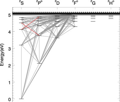
(a)

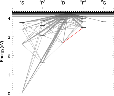
(b)

Figure 1: Grotrian diagram of Na  (upper panel) and K  (lower panel) model atoms used in this work. The red lines correspond to transitions in the $H$-band.

The final model atom of Na  has 42 levels of Na i and the ground level of Na ii, and a total of 190 radiative transitions. while for K  we used 31 levels of K i and the ground level of K ii and a total of 219 radiative transitions. Figure 1 shows the Grotrian diagram with the levels and the transitions of the K  and Na  model atoms used in this work.

2.2.1 Energy levels and radiative data

Energy levels for Na i  and K i were adopted from NIST. Fine structure components were ignored while the allowed angular momentum components lower than $l=6$ for a given principal quantum number $n$ were taken as separated levels up to $n=8$ for Na  and $n=6$ for K . $n$ super levels were included up to $n=20$ for Na  and K  in order to assure coupling between the highest level of the neutral species and the ground level of their first ion.

Photo-ionisation cross-sections of Na i were taken from the TOPBASE data base. K i photo-ionisation data were taken from Zatsarinny & Tayal (2010). When bound-free data were not available, photo-ionisation cross-sections were calculated using the hydrogenic formula implemented in TLUSTY (Hubeny & Lanz, 1995, for recent upgrades, detailed description and users’ manual, see Hubeny & Lanz (2017a, b, c)).

Oscillator strengths (f-values) come from various sources collected in the NIST and VALD data bases. TOPBASE (Cunto & Mendoza, 1992), provide the atomic data (f-values, photo-ionisation cross sections) from the Opacity Project calculations (Seaton, 1996). For Na , VALD has the experimental f-values provided by NIST so the Na  f-values from VALD have priority over NIST. For the rest of bound-bound transitions TOPBASE data were used when available. In the case of K , data from VALD come from Kurucz (2012) while data from NIST is mostly from Sansonetti (2008). When for the same transition, f-values from different sources differ, preference was given to NIST over VALD in this case. VALD also provides collisional broadening parameters from Kurucz (2012) and Barklem et al. (2000) where available. Line broadening data are taken from Barklem et al. (2000), via VALD, when available. Otherwise we adopted the formula from Unsöld (1955) with an enhancement factor of 2, as suggested by Mashonkina et al. (2000) in their Na NLTE studies on the Sun. Radiative bound-bound data for the most important transitions of Na  and K  (including those in the APOGEE window) are presented in Table 1.

Table 1: Data adopted for the NLTE Calculations for characteristic lines of Na  and K .

low (J)	Upp (J)	$\lambda$[Å]	loggf	log $\Gamma_{4}$	log $\Gamma_{6}$
Na i
3s(1/2)	3p(1/2)	5 895.9	-0.194	-5.64	-7.53*
3s(1/2)	3p(3/2)	5 889.9	0.108	-5.64	-7.53*
3p(3/2)	3d(1/2)	8 183.3	0.237	-5.38	-7.23*
3p(3/2)	3d(1/2)	8 194.8	0.492	-5.38	-7.23*
3p(1/2)	4d(1/2)	5 682.6	-0.706	-4.52	-6.85*
3p(3/2)	4d(3/2)	5 688.2	-0.452	-4.52	-6.85*
3p(1/2)	5s(1/2)	6 154.2	-1.547	-4.39	-6.99
3p(3/2)	5s(3/2)	6 160.7	-1.246	-4.39	-6.99
3p(1/2)	6s(1/2)	5 148.8	-2.044	-5.59	-6.81
3p(3/2)	7s(3/2)	4 751.8	-2.078	-5.63	-6.67
4s(1/2)	5p(3/2)	10 746.4	-1.294	-5.97	-6.91
4p(1/2)	6s(1/2)	16 373.9	-1.328	-4.23	-6.84
4p(3/2)	6s(1/2)	16 388.8	-1.027	-4.23	-6.84
5s(1/2)	8p(3/2)	16 393.9	-2.149	-3.14	-6.52
5s(1/2)	8p(1/2)	16 395.2	-2.456	-3.14	-6.52
K i
4p(1/2)	7s(1/2)	5 782.4	-1.909	-4.11	-6.79
4p(3/2)	7s(1/2)	5 801.8	-1.605	-4.11	-6.79
4p(1/2)	6s(1/2)	6 911.1	-1.409	-4.52	-6.91*
4p(3/2)	6s(1/2)	6 938.8	-1.252	-4.52	-6.90*
4s(1/2)	4p(3/2)	7 664.9	0.127	-5.64	-7.44*
4s(1/2)	4p(1/2)	7 699.0	-0.177	-5.64	-7.44*
4p(1/2)	5s(1/2)	12 432.3	-0.444	-5.06	-7.34*
4p(3/2)	5s(1/2)	12 522.2	-0.135	-5.06	-7.34*
3d(5/2)	4f(7/2)	15 163.1	0.617	-4.79	-6.82
3d(3/2)	4f(5/2)	15 168.4	0.494	-4.79	-6.96

2.2.2 Collisional data

Electron collisions. The formula from Park (1971), which is an empirical adjustment of the Born approximation applicable only to neutral alkali atoms, has shown to be a good approximation for NLTE calculations of Li and Na in cool stars when compared with more sophisticated data (Osorio et al., 2011; Lind et al., 2011). For Na , the convergent close coupling (CCC) calculations from Igenbergs et al. (2008) cover all transitions for the levels up to $4f$ and those where included in our model atom. Regarding K , very recent calculations from Reggiani et al. (2019) suggest that the Park formula tends to overestimate the K  collisional rates. They perform CCC and B-spline R-matrix (BSR) calculations (both agree extremely well) for electron collisional excitation between all levels up to $6d$; we decided to adopt their BSR data.

We filled the missing transitions of Na in Lind et al. (2011) and of K in Reggiani et al. (2019) with the Park formula. It covers all the transitions between levels up to n=7 for Na  and n=6 for K . For higher levels, it provides data for transitions between the 16 closest levels with n${}_{upper}\leq 20$. For the remaining transitions, the formula from Seaton (1962) was implemented.

Electron collisional ionisation was described via the hydrogenic approximation as presented in Cox (2000, Sect 3.6.1) for low-lying levels, and the formula from Vrinceanu (2005) for levels with principal quantum number $n\geq 5$ for Na  and $n\geq 6$ for K .

Hydrogen collisions. For collisional excitation of Na  and K  we adopted data from Barklem et al. (2012) and Barklem (2016, 2017a) respectively. Those works cover the transitions between all levels from the ground state up to 5p for Na  and 4f for K . For the missing one-electron transitions in these works, hydrogen collisional excitation was calculated using the code from Barklem (2017b) based on the free electron model of Kaulakys (1985, 1986).

Charge transfer processes like $\rm{A}+\rm{H}\leftrightarrow\rm{A}^{+}+\rm{H}^{-}$ were calculated by Barklem et al. (2012) and Barklem (2016, 2017a) for Na  and K  respectively and are included in this work.

Figure 2 shows the rate coefficients obtained at 5 000 K for the different collisional processes described above for the Na  and K  atoms. It is important to remember that the rate coefficients are an estimation of the efficiency of the transition, and the actual rate of a transition is obtained multiplied multiplying by the population of the projectile. For solar metallicities the population of hydrogen is around four orders of magnitude larger than the population of free electrons, and therefore even if the rate coefficients for electron collisional excitation is one or two orders of magnitude stronger than their hydrogen counterpart, the contribution to the total collisional excitation rate from hydrogen collisions can be more important than the contribution from electron collisions. At lower metallicities, fewer free electrons are available, weakening even more their contribution to the total collisional rate and thus making the hydrogen contribution even more important.

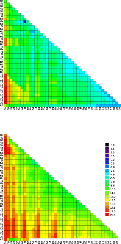
(a)

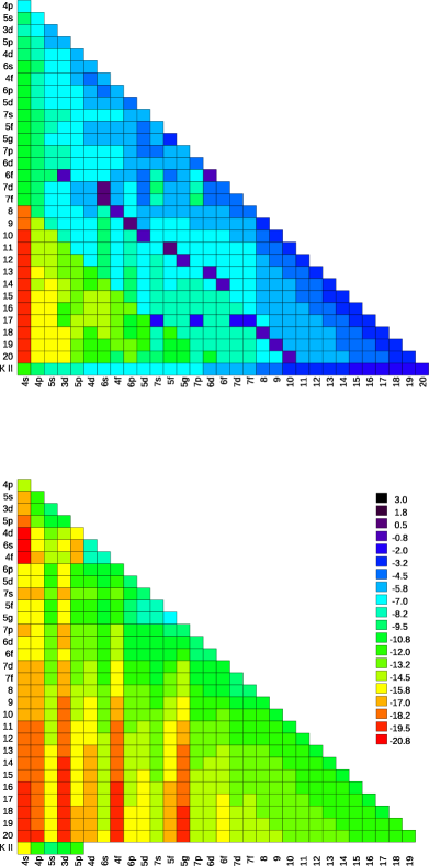
(b)

Figure 2: Rate coefficients of the electron related collisions (excitation and ionisation, top ) and hydrogen related collisions (excitation and charge-exchange, bottom) for Na  (left) and K  (right). Initial levels of the transitions are labelled in rows and final levels are labelled in columns. The arrows point towards the transition that separates the hydrogen collisional excitation data from Barklem et al. and the data calculated using the formula from Kaulakys (1985). The colour scale at the left is for the Na  rates and the colour scale at the right is for the K  rates.

2.3 The APOGEE spectral window

NLTE effects are different for different lines, and when the atomic lines to be observed are from transitions involving higher levels, having high quality collisional data for the low lying levels (which are the most populated) is important. However, one also must pay special attention to the collisional data for transitions associated with the lines of interest. For that reason, the study of the $H$-band (where most of the atomic transitions are between high excitation levels) requires the model atoms of the elements under study to have enough high-lying levels and the collisional data for transitions involving those levels to be as good as possible. Unfortunately, modern calculations of collisional excitation and ionisation usually do not cover such transitions.

We have built our model atoms with those concerns in mind. The levels used in the final model atom are such that the lines in the $H$-band do not involve transitions between super levels, required to keep the size of the model atom manageable, and at the same time have a realistic coupling with the continuum (Mashonkina, 2010; Asplund, 2005). Most of the collisional (de-) excitation data for the transitions in the $H$-band, and the collisional ionisation data for levels involved in those transitions, are outside the cover of modern, detailed, quantum mechanical calculations. Recent studies (and some not-too recent but not commonly used) give us better alternatives to the old, traditional approximations methods. The above considerations demonstrate that we put considerable effort in the adoption of the best data available for transitions involving high-lying levels, as it is the case for many of the lines in the $H$-band.

2.4 Reference stars

We decided to use the Sun, Arcturus and Procyon for the comparison between observations and our synthetic spectra. The observational data used in this work are the same as the ones described in Osorio et al. (2019). Here, we can mention that our selection was based on the excellent quality of the data and the reliability of the atmospheric parameters, together with the wide wavelength coverage of the observations.

For Procyon, we used the observations from PEPSI (Strassmeier et al., 2018). Its wavelength coverage is (3 800 - 9 100 Å) at R$\sim 220\,000$. The solar observations we used were the 2005 version of the flux atlas from Kurucz et al. (1984), it covers from 30̇00 to 10 000 Å, with a full width half maximum reducing power R$\sim 400\,000$. For Arcturus we adopted the atlas from Hinkle et al. (2000) that spans from 3 727 to 9 300 Å and has R$\sim 150\,000$. A more detailed description of the observations and a comparison with other atlases can be found in Osorio et al. (2019). The atmospheric parameters adopted are given in Table 2. For more details regarding the observational data please refer to Osorio et al. (2019).

Table 2: Parameters of the model atmospheres used for the construction of the synthetic spectra.

Name	$T_{\mathrm{eff}}$[K]	$\log\,g$ [cm s-2]	[Fe/H]	vmic[km s-1]
Procyon†	$6\,530$	$4.00$	+0.0	2.00
Sun††	$5\,772$	$4.44$	+0.0	1.10
Arcturus†††	$4\,247$	$1.59$	$-$0.5	1.63

3 Computations

There are two sets of computations done in this work: in the first one we used the results of the well-established NLTE radiative transfer code for cool stars MULTI (Carlsson, 1986, 1992), and compare its results with the last version of TLUSTY (Hubeny & Lanz, 1995, 2017a, 2017b, 2017c) that now allows for the calculation of NLTE populations in cool stellar atmospheres. Given that TLUSTY was created for the study of early-type stars and accretion discs, it allows for the treatment of multiple species in NLTE at the same time; a property long known to be necessary for NLTE studies in hot stars (Auer & Mihalas, 1969a). We obtained Mg and Ca LTE/NLTE populations with the two codes using the same input atomic data and a configuration as similar as possible to each other. The results and analysis of these calculations are given in §4.

The second set of computations are performed exclusively with TLUSTY (to calculate the LTE/NLTE populations) and SYNSPEC (to calculate the detailed spectra). We compare observations against the results of two different NLTE calculations: the traditional (for cool stars) trace-element, single-species NLTE calculation, referred to as NLTE-s, and calculations where multiple species are treated in NLTE simultaneously, still within the trace-element framework, referred to as NLTE-m. We used Arcturus, the Sun and Procyon to calculate the LTE, NLTE-s, and NLTE-m populations and spectra of Na, Mg, K and Ca on these stars. From §5 on, this paper is dedicated to the second set of computations.

The NLTE-m calculations are a better approximation than the NLTE-s ones from the physical point of view: the effects of the NLTE radiation of one atomic species on the NLTE populations of other species is included in the NLTE-m and ignored in the NLTE-s calculations. The relevance of such effects in cool stars is studied for the first time in this work (see §5.1).

In order to obtain the NLTE populations we ran TLUSTY v.207 in the opacity table mode. The opacity tables were constructed using SYNSPEC v.53. After experimentation with different numbers of wavelengths, temperatures and densities, the adopted table for the second set of calculations has 100 000 wavelength points equally distributed in a logarithmic scale from 900 to 100 000 Å; 10 temperature grid points and 10 density grid points. The element abundances used in the the opacity tables are the appropriate for each star’s metallicity. In each NLTE calculation, the opacity table used excludes the contribution from the elements treated in NLTE.

The detailed synthetic spectra (in LTE and NLTE) were calculated using the same code as the opacity tables SYNSPEC v.53, adopting the same atomic and molecular line-list as in Mészáros et al. (2012) but with $\log gf$ and broadening parameters of the Na i, Mg i & ii, K i and Ca i & ii lines replaced by the ones used in the NLTE calculations done with TLUSTY.

The stellar model atmospheres are the same as in Osorio et al. (2019): Kurucz model atmospheres computed with ATLAS9 (Kurucz, 1993), using the setup described in Mészáros et al. (2012).

4 Comparison between TLUSTY and MULTI

The last updates of TLUSTY bring the possibility to use the code for NLTE calculations for a subset of species, while the rest of atomic, as well as molecular, species are treated through pre-calculated opacity tables. We can thus compare with other NLTE radiative transfer codes used in the study of cool stars.

Our first goal was to reproduce the results obtained in previous works, more precisely the solar departure coefficients obtained for Mg (Osorio et al., 2015) and Ca (Osorio et al., 2019). In both cases the calculations were performed with the NLTE radiative transfer code MULTI (Carlsson, 1986) version 2.3; and now we repeat the calculations with TLUSTY. The results of such comparison are shown in this section.

The same solar model atmosphere used in Osorio et al. (2019) is adopted here for both Mg and Ca. The input data for Mg and Ca used in both MULTI and TLUSTY were adapted for each code and this adaptation led to the differences described in §4.2, 4.3 and 4.4.

4.1 Background opacity

In this work we use the term background opacity to refer to all the sources of opacity that do not involve the elements under study. In TLUSTY, those are stored in pre-calculated opacity tables. In MULTI, the continuous opacities are calculated on-the-fly, while only line opacities are stored in a read-in file (line-opacity table).

For MULTI, we used a line-opacity table based on the background opacities presented in Gustafsson et al. (2008) re-sampled to 10 300 frequency points between 900 and 200 000 Å. The bound-free (b-f) and free-free (f-f) contribution from the most important atomic elements and also the b-f and f-f contribution from several molecules are calculated by the code.

Unlike previous versions, the latest version of TLUSTY allows the use of opacity tables. These tables include also the bound-bound (b-b) contribution from atoms and some molecules. In order to make the comparison easier, the opacity tables used in TLUSTY for this test have the same number of frequency points and wavelength coverage than those adopted for the MULTIcalculations. The atoms and molecules that contribute to the background opacities are listed in Table 3. A sample of the background opacities used for the Mg NLTE calculations in MULTI and TLUSTY is presented in Fig. 3.

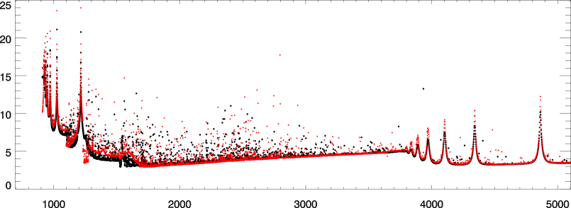
(a)

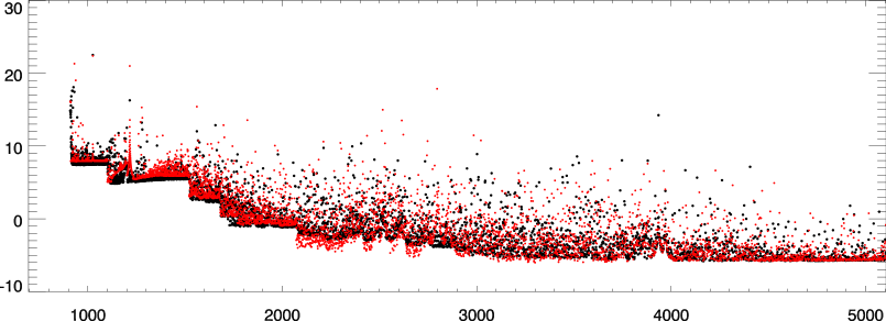
(b)

Figure 3: Sample of the background opacities from the opacity tables in the UV region used in the NLTE calculation of Mg (i.e., removing the contribution of Mg .) by MULTI (red) and TLUSTY (black) at two different points of the solar atmosphere.

Table 3: Components of the background opacities used for the comparison calculations between MULTI^∗ and TLUSTY.

Species	Process
	MULTI		TLUSTY
H -	bf, ff		bf, ff
H i	bb, bf, ff		bb, bf∗∗, ff
He i	bb, bf, ff		bb, bf, ff
He -	ff		bf, ff
C i & ii	bb, bf		bb, bf, ff
C -	ff
N i & ii	bb, bf		bb
N -	ff
O i & ii	bb, bf		bb, bf, ff
O -	ff
Na i & ii	bb		bb, bf, ff
Mg i†	bb, bf, ff		bb, bf, ff
Mg ii†	bb, bf		bb, bf, ff
Al i & ii	bb		bb, bf, ff
Si i	bb, bf, ff		bb, bf, ff
Si ii	bb, bf		bb, bf, ff
K i	bb		bb, bf, ff
Ca i & ii†† bb	bb, bf		bb, bf, ff
Fe i & ii	bb, bf		bb, bf, ff
All other metals	bb, ff		bb
H ${}^{+}_{2}$	ff		ff
H ${}^{-}_{2}$	ff
CH & bf		bb, bf
OH & bf		bb, bf
CO & bf		bb
Other diatomic molecules†††	bb		bb
H    Rayleigh Scattering	yes		yes
He Rayleigh Scattering	yes		yes
H 2 Rayleigh Scattering	yes		yes
e- (Thomson) Scattering	yes		yes

4.2 Photo-ionisation

The source of the data for Mg and Ca is the TOPBASE database (Cunto & Mendoza, 1992). For the MULTI calculations, the data were used directly with the exclusion of some values. A maximum of 500 points per b-f transition (starting from threshold) were used. If, for a given level, the cross section extended to energies higher than 13.6 eV (corresponding to 911 Å), those data points were removed, since the lowest wavelength in the line-opacity table used by MULTI is 900 Å. This applies to all photo-ionisation cross sections, except the one of the ground level of Mg ii because its threshold is at 14.3 eV (870 Å, see Fig. 4) and according to the above criteria, the whole cross section for this level would have been removed in the MULTI calculations. Having the b-f taken directly makes it possible to have the resonances present in the data fully resolved for photon energies near the threshold.

For TLUSTY, the original TOPBASE data were smoothed and re-sampled using the resonance averaged photo-ionisation cross sections method presented by Bautista et al. (1998). This smoothing is physically justified given the uncertain in the atomic structure calculations, but it also brings a benefit due to the reduction in the number of frequencies required to describe the cross-sections. For these calculations, we used the full wavelength range provided by the sources for all the b-f transitions. Figure 4 shows the photo-ionisation data used for two levels of Mg i in the TLUSTY (symbols in black) and MULTI (red lines) codes.

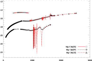
(a)

Figure 4: Photo-ionisation cross section data used in the MULTI (red lines) and TLUSTY (black symbols) calculations for two b-f transitions of Mg i and the one from the ground level of Mg ii. The red lines are the values taken from the TOPBASE database with the cross sections bellow 911 Å removed (except for the Mg ii b-f transition). The symbols are the resonance averaged photo-ionisation cross sections of the TOPBASE data (see Allende Prieto et al., 2003). The b-f cross section of the Mg ii 3s(2S) and the Mg i 3p(3P) levels are vertically shifted 4 and 2 log units respectively in order to ease visualisation.

4.3 Van der Waals broadening

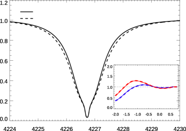
(a)

Figure 5: Comparison between MULTI NLTE solar line profile and departure coefficients (inner figure) of the levels involved for the Ca i transition 4p¹P - 4s¹S (4227 Å); when the Van der Waals broadening is treated using the ABO theory (solid lines) and when the formulation from Unsöld (1955), with a $\Gamma_{6}$ value derived from the ABO theory, is used (dashed lines).

When available, MULTI uses the ABO theory directly by having the Van der Walls broadening input data in the ”$\sigma.\alpha$” format. TLUSTY, on the other hand, uses the Van der Waals broadening coefficient $\Gamma_{6}$ at 10 000 K. When available, the values adopted for TLUSTY are the equivalent $\Gamma_{6}$ at 10 000 K obtained from the ABO theory. This difference in the treatment of the spectral lines does not affect the derived NLTE populations, but it affects the line profiles. We have compared two MULTI calculations: one using the ABO theory and the other treating van der Waals damping with the Unsöld method (Unsöld, 1955) with an$\Gamma_{6}$ at T=10 000 K derived from the ABO theory, and found no differences in the NLTE populations, although the wings of line profiles are clearly different (see Fig. 5). Therefore, the differences between the line profiles of MULTI and TLUSTY/SYNSPEC for lines with ABO format data lie in the line-profile calculations between MULTI and SYNSPEC, and not in the NLTE populations derived by MULTI and TLUSTY. This is easy to understand because possible departures form LTE a driven by radiative rates, which in turn are dominated by the line cores.

4.4 Collisional data

MULTI requires upward rate coefficients for transitions resulting in ionisation and downward rate coefficients for transitions resulting in excitation, while TLUSTY demands upward collisional rate coefficients in all cases. We used detailed balance relations in order to convert upward $\leftrightarrow$ downward rate coefficients (see Hubeny & Mihalas, 2014, §9.3).

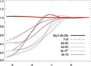
(a)

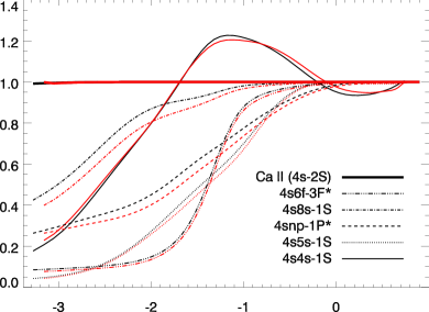
(b)

Figure 6: Departure coefficients for some levels of Mg i (upper panel) and Ca i (lower panel) obtained with TLUSTY (red) and MULTI (black) for the same solar model atmosphere and the same atomic data. The grey vertical lines denote the depths at $\tau_{ross}=0.01$ (left) and $\tau_{ross}=1.0$ (right).

4.5 Results of the comparison

The most direct comparison between these two codes is done by comparing the NLTE populations through the departure $b$ coefficients as function of the column mass. Traditionally, departure coefficients as shown as a function of optical depth $\tau$, but given that $\tau$ depends more on the background opacities (which is not exactly the same in TLUSTY and MULTI) than the column mass, and because the calculations in both codes are performed in the column mass scale, a more direct comparison between the two codes can be made using column mass as abscissae. Figure 6 compares the obtained departure coefficients of some levels of Mg  and Ca  against column mass for a solar model. The behaviour is very similar for the two codes (see top panel of Fig. 6). The small discrepancies are due mainly to the differences in the background opacities. Figure 6 gives us confidence on the ability of the new version of TLUSTY to perform NLTE calculations in late-type stars.

Our experiments show that certain level of detail in the background opacities is required for calculating reliable NLTE populations. It is also important to ensure that the adopted background opacities cover the wavelengths associated to the most important b-b and b-f transitions of the species computed in NLTE. A more detailed comparison between TLUSTY and other NLTE-trace-element radiative transfer codes will be presented in a future paper.

5 Multi-element NLTE radiative transfer

In what follows we will label as NLTE-s the traditional single-element NLTE calculations (i.e. where only one atomic element was calculated in NLTE while all the other elements were kept in LTE) and NLTE-m to the simultaneous multi-element NLTE calculations.

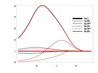
(a)

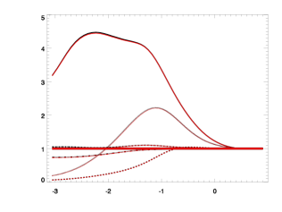
(b)

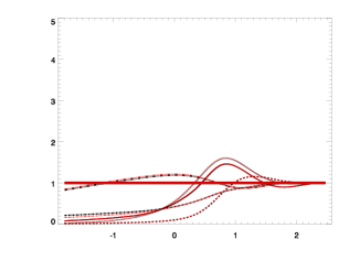
(c)

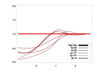
(d)

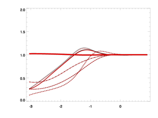
(e)

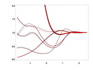
(f)

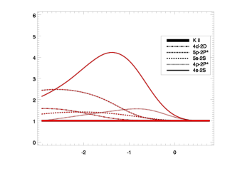
(g)

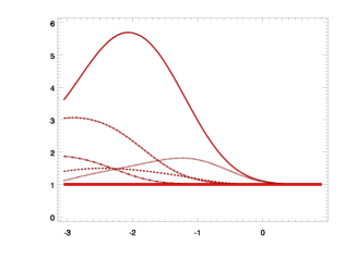
(h)

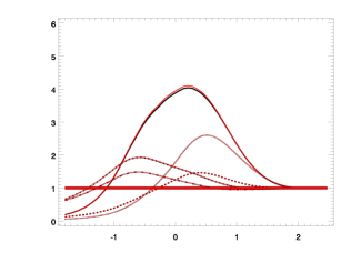
(i)

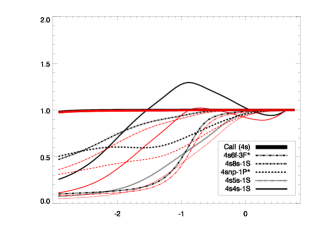
(j)

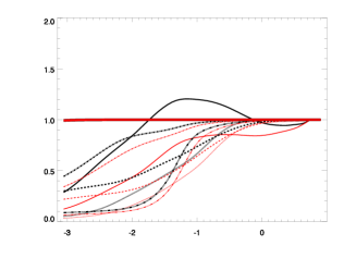
(k)

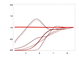
(l)

Figure 7: Departure coefficients for some levels of Na ,  Mg ,  K  and Ca  obtained calculated in single-element mode (NLTE-s, in red) and in multiple-elements mode (NLTE-m, in black) for Procyon, the Sun and Arcturus. For each star, the same element abundances were used in all the LTE, NLTE-s and NLTE-m calculations.The fact that the $b$ coefficient for the Mg ii ground state increases toward the surface (due to NLTE effects in the Mg ii h & k lines) in Arcturus, but stays closely to 1 for the other two stars, follows from Mg ii being the dominant stage of ionisation, and its ground state the most populated state, for Sun and Procyon, but not for the cooler star Arcturus. The two grey vertical lines in each figure mark the depths in the atmospheres where $\tau_{ross}$=0.01 (left) and 1.0 (right)

We performed NLTE-s calculations for Na ,  Mg ,  K  and Ca . We also performed NLTE-m calculations with all possible combination of two, three and the four elements in NLTE. As a result we found that departures from LTE in Mg  is affecting mainly the Ca  populations but does not have significant effects on Na  or K . Ca  has a marginal effect on Mg , especially in Arcturus, but in this star NLTE effects in Mg  have a diminished influence on the NLTE Ca  populations. Na  and K  are not affecting the populations of each other, Mg  or Ca  in any of the stars investigated in this work.

We emphasise that all the calculations described have been performed with exactly the same atomic data: the opacity tables used for the different NLTE-s and NLTE-m calculations are constructed exactly in the same fashion with the exact same b-b and b-f data, only removing the contribution to the opacity of the elements to be calculated in NLTE. The model atoms of Mg i & ii and Ca i & ii for MULTI have the same radiative and collisional sources than the ones used for TLUSTY (the differences in the data implemented in the two codes are described in § 4). The same Na i, Mg i & ii, K i and Ca i & ii model atoms where used in all the NLTE calculations in TLUSTYand SYNSPEC. Thus, the differences found in the NLTE-s and NLTE-m populations and spectra are due only to inter-element NLTE effects.

Given that in all the calculations we keep fixed the atmospheric structure i.e., we are still within the trace-element approach framework, the influence of one NLTE element on the others enters trough its contribution to the opacity. A comparison of the NLTE departure coefficients $b$ between the NLTE-s and NLTE-m cases can give us information on the importance of inter-element NLTE effects (see below).

5.1 Inter-element NLTE effects

Our experiments show that the Ca  NLTE populations are sensitive to Mg  NLTE opacities, but the Mg  NLTE populations are not affected by Ca  NLTE opacities significantly. This opens the question of how much the effect of Fe NLTE opacities will affect the NLTE effects of other elements considering that Fe is the metal that contribute the most to background opacities at solar metallicities, in particular in the UV region. We now proceed to interpret the behaviour of NLTE-m with respect to NLTE-sin the stars and atomic elements studied in this work.

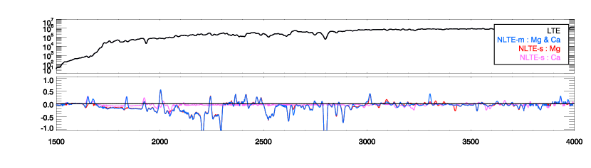
(a)

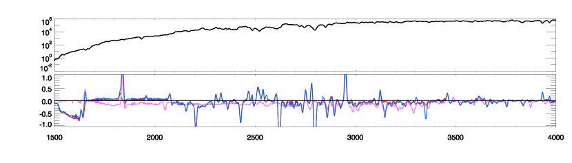
(b)

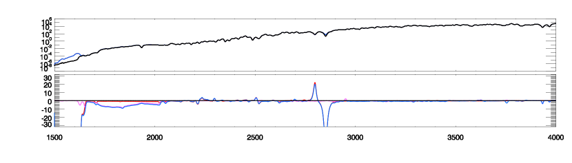
(c)

Figure 8: UV fluxes obtained for Procyon (top), the Sun (middle) and Arcturus (bottom) calculated in LTE (black), NLTE-m (red) NLTE-s:Mg (pink) and NLTE-s:Ca (blue). For each star, the Eddington flux (upper panel) and the % difference between the LTE and the NLTE fluxes (lower panel) are plotted. The units of the Eddington flux $H_{\lambda}$ are erg cm^-2s^-1Å^-1.

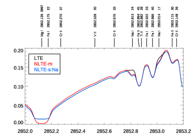
(a)

Figure 9: LTE (black), NLTE-m(red) and NLTE-s:Na (blue) normalised synthetic fluxes of Procyon around the red wing of the 2852 Å Mg i line. The atomic species of some lines are marked together with its LTE equivalent width in mÅ.

5.1.1 Procyon

In the case of Procyon the interplay between Mg  and Ca  leads to an increase of the NLTE flux in the $\sim$2 000-2 300 Å region, which is the location of the photo-ionisation threshold of the ground level of Ca i (2 028 Å). Thus, the resulting background UV opacity seen by Ca  is different between the NLTE-s:Ca and the NLTE-m calculations. Photon loss competes with over-ionisation, but at column-mass $\sim-1$ the overpopulation of the Mg i lower levels in NLTE with respect to LTE reduces the UV flux in those layers giving advantage to photo loses of the resonance Ca i lines ($\sim$2 500 Å and 4 226.7 Å) which results in an increase of the population of the lowest levels of Ca  in NLTE-m with respect to NLTE-s:Ca (i.e., when Mg  is treated in LTE). In contrast, Mg  seems to be affected very little by Ca  and its NLTE populations are almost identical in the NLTE-s and NLTE-m calculations. Regarding the alkali elements; given that the main NLTE mechanism driving the statistical balance of Na  and K  is photon-suction, these elements are unaffected by the changes in the UV flux due to the Mg  NLTE populations. As we mentioned at the introduction of this subsection, the 3s(²S) and 5p(²P_1/2, 3/2) are the levels involved in the the 2852 Å Na  lines. Their departure coefficients change due to differences in the background opacity given that these lines are in the red wings of the 2852 Å Mg i line, whose formation in NLTE is not the same as in LTE.

5.1.2 Sun

As in the case of Procyon, the UV flux in the NLTE-m calculations is very similar to the NLTE-s:Mg calculations, so again Ca  is much more sensitive to Mg  than Mg  to Ca . The main difference in departure coefficients between NLTE-s:Ca and NLTE-m results are on the ground level of Ca i because a similar process to the one occurring in Procyon takes also place in the Sun, and in this case it is enhanced due to the broader lines that favour photon losses. The UV synthetic spectra show that the flux of the NLTE-s:Mg and NLTE-m are very similar (middle panel of Fig.8) and thus the departure coefficients of Mg  in the two cases are almost identical. Na  and K  have NLTE effects driven by photo-suction making their departure coefficients of the NLTE-s and NLTE-m calculations almost identical.

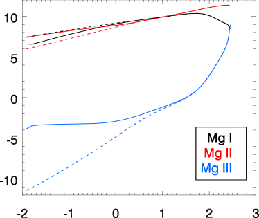
(a)

Figure 10: Mg  number densities of different ionisation stages in Arcturus. The solid lines represent the NLTE populations while the dashed lines represent the LTE populations.

5.1.3 Arcturus

Mg i is not a minority species anymore in the atmosphere of Arcturus; in fact, at column-mass $\lesssim 1$ the population of Mg i is larger than the population of Mg ii, as illustrated in Fig. 10. Since there is not a Mg ii reservoir in Arcturus any more, photo-ionisation of the 3p(1P^∗) level is not efficient compared with the photon pumping that occurs in the 3p(1P)-3s(1S) Mg i line at 2 850 Å, making this level to have $b>1$ along the atmosphere (see Mg in Arcturus panel in Fig. 7).

As seen in Fig. 8, the NLTE-m UV fluxes are now more influenced by Ca  than by Mg  in some regions (like the 1 700 - 2 000 Å ). But the UV flux in Arcturus is three to four orders of magnitude weaker than in the Sun, thus the absolute changes in the UV fluxes due to the NLTE populations of Ca  and Mg  are not large enough to affect the NLTE-m populations of the four atomic elements significantly with respect to their NLTE-s populations. On the other hand, due to the lower gravity of Arcturus, metallic lines broaden, so lines with different NLTE / LTE behaviour in the wings (mostly resonance lines) will also affect a larger part of the spectrum than in case of dwarfs. This explains why the departure $b$ coefficient of the ground level of K  has an small but noticeable NLTE-m/NLTE-s difference in Arcturus and no difference in the Sun and Procyon.

Ca i, on the other hand, is still a minority species in Arcturus and thus UV over-ionisation still dominates, but since the UV is much weaker than in the other two stars, the effects of NLTE Mg  opacities on the NLTE Ca  populations is not as strong as in the solar and Procyon cases (see Fig. 7).

5.2 Physics of the inter-element effects

Na  and K  are not affected by any of the other elements. We note though, that the Na i levels 3s(²S) and 5p(²P) have slightly different departure $b$ coefficients between the NLTE-s and NLTE-m calculations, in particular for Procyon. The transition between those levels produces the 2 852.8 and 2 853.0 Å lines, which lie in the red wing of the Mg i 2 852 Å line. This is an illustration of how the NLTE opacities of some elements can affect the statistical balance of other elements: the background opacity at around 2 853  Å is dominated by the red wing of the Mg i 2 852 line, which has different strength along the stellar atmosphere when Mg  is treated in NLTE and in LTE (see Fig. 9). The differences observed between the red (NLTE-s) and black lines (NLTE-m) in Fig. 7 are the result of the combination of the overlap between b-b and b-f transitions of the different elements treated in NLTE, like the one just mentioned.

Given that the main NLTE mechanism affecting the Ca  and Mg  populations is UV over-ionisation, the differences between the NLTE-s and NLTE-m populations for both Ca  and Mg  come mostly from their effects on the radiation field of that region. Figure 8 helps to understand the differences between the departure coefficients $b$ shown in Fig. 7. The figure shows three panels (one for each star) with the absolute flux obtained in LTE, NLTE-m, and NLTE-s for Mg  and Ca  at the top and the percentage difference between the LTE flux and the three NLTE fluxes (single and multi element) at the bottom of each panel. Broad lines with wings affected by NLTE will affect lines of other elements with lines formed the wings because their background opacity will have a contribution of the NLTE wings. For the Sun and hotter stars, the UV flux is strong enough to affect species sensitive to over-ionisation in NLTE-m if there are other species in the calculations that affect the continuum fluxes due to NLTE effects. Our results show also that, NLTE effects on broad lines will result in different background opacities perceived by lines of other elements in the same region, potentially affecting the NLTE results of those other elements.

The fundamental effect of NLTE calculations is the redistribution of the population of different levels in the different ions of a given element, with respect to LTE. As a consequence for an element X, spectral lines and the continuum contribution is different in LTE and NLTE for an atmosphere with the same X abundance. That is the reason why even though the derived LTE and NLTE Mg  solar abundance is the same, the derived NLTE-s and NLTE-m abundances of Ca  are different. Figure 9 illustrate this; the Mg  abundance used in the three profiles shown is the same (A(Mg)=7.42 dex) and the LTE and NLTE-s:Na calculations provide the same profile of the broad 2852 Å Mg i line, the NLTE core and wings of this line differs in the NLTE-m Calculations since Mg  is now in NLTE with the same A(Mg ). The reason for the different profiles in LTE and NLTE is due to the redistribution of the population of the levels involving that transition (3p ¹P - 3s ¹S) that leads to a deeper core and weaker wings of the Mg  NLTE profile with respect to the Mg  LTE line profile.

6 Comparison with observations

Finally we derived Na , Mg , K  and Ca  abundances for Procyon, the Sun and Arcturus in LTE, NLTE-s and NLTE-m. The derived abundances and macro-turbulent velocities are presented in Table 4.

Table 4: Na , Mg , K  and Ca  abundances derived for the LTE, NLTE-s and NLTE-m calculations. Macro-turbulent velocity was also a free parameter in each calculation. The second column shows the number of points used to perform the best fit calculation.

Star		LTE			NLTE-s			NLTE-m
	N	A(X)	Vmac	$\chi^{2}$	A(X)	Vmac	$\chi^{2}$	A(X)	Vmac	$\chi^{2}$
Na
Procyon	935	6.36$\pm$0.09	2.87$\pm$1.44	0.92	6.14$\pm$0.05	6.68$\pm$0.85	0.25	6.13$\pm$0.05	6.69$\pm$0.86	0.25
Sun	2358	6.29$\pm$0.05	1.45$\pm$4.19	8.09	6.15$\pm$0.04	1.25$\pm$1.28	4.35	6.15$\pm$0.04	1.25$\pm$1.29	4.35
Arcturus	501	5.91$\pm$0.06	2.18$\pm$2.30	0.65	5.80$\pm$0.05	3.82$\pm$1.33	0.62	5.80$\pm$0.05	3.81$\pm$1.32	0.62
Mg
Procyon	2504	7.42$\pm$0.06	6.52$\pm$1.77	1.14	7.42$\pm$0.05	7.10$\pm$1.45	1.03	7.42$\pm$0.05	7.12$\pm$1.46	1.02
Sun	2729	7.56$\pm$0.02	2.32$\pm$2.28	1.86	7.56$\pm$0.02	3.36$\pm$1.55	1.40	7.56$\pm$0.02	3.38$\pm$1.55	1.40
Arcturus	1192	7.40$\pm$0.05	3.93$\pm$1.68	3.26	7.39$\pm$0.05	5.13$\pm$1.19	3.02	7.39$\pm$0.05	5.16$\pm$1.20	3.03
K
Procyon	120	5.71$\pm$3.06	2.32$\pm$1.56	0.06	5.05$\pm$0.04	5.60$\pm$0.26	0.01	5.05$\pm$0.04	5.60$\pm$0.26	0.01
Sun	182	5.36$\pm$0.07	0.99$\pm$1.03	0.04	5.09$\pm$0.04	1.30$\pm$1.10	0.01	5.09$\pm$0.04	1.30$\pm$1.10	0.01
Arcturus	182	4.98$\pm$0.05	3.95$\pm$0.30	0.02	4.54$\pm$0.04	5.25$\pm$0.20	0.02	4.55$\pm$0.05	5.23$\pm$0.20	0.02
Ca
Procyon	1410	6.17$\pm$0.07	3.68$\pm$1.12	2.78	6.13$\pm$0.06	5.01$\pm$0.81	2.23	6.10$\pm$0.06	4.95$\pm$0.74	2.27
Sun	6116	6.35$\pm$0.05	0.77$\pm$1.77	5.92	6.37$\pm$0.05	0.71$\pm$1.76	4.76	6.30$\pm$0.04	0.69$\pm$1.57	3.93
Arcturus	2026	5.97$\pm$0.08	3.28$\pm$1.36	7.88	5.99$\pm$0.08	3.60$\pm$1.20	8.81	5.98$\pm$0.08	3.61$\pm$1.10	8.80

We used the all-lines method described in Osorio et al. (2019), where all the lines of the spectrum were analysed simultaneously; therefore a single abundance and macro-turbulent velocity was used for all the lines of a given element simultaneously. In order to determine the error associated with the derived abundances and macro-turbulent velocities, we used the method described in section 5 of Piskunov & Valenti (2017) where the model errors are prioritised. For all the three stars and the four elements studied in this work, the residuals ($\chi^{2}$) of the best fit in NLTE are reduced relative to the LTE analysis, except for Ca  in Arcturus (we found the same anomaly in Osorio et al.). The $\chi^{2}$ of the NLTE-m calculations is either lower or the same as the $\chi^{2}$ of NLTE-s calculation. The case of Ca  in the Sun is particularly interesting: while its NLTE-s abundance correction is marginally positive (0.02), the NLTE-m abundance correction is negative (-0.05) and the NLTE-m abundance becomes in excellent agreement with the meteoritic value. A more detailed description is given below.

The closest comparison of our results and previous works are for Na Lind et al. (2011), for Mg Osorio et al. (2015), for K Reggiani et al. (2019) and for Ca Osorio et al. (2019). The LTE / NLTE-s results are generally in very good agreement with those studies considering the differences in methodology (equivalent with vs line profile fitting, line-by-line abundance determination vs all-lines at once, etc) and the input data used (different model atmospheres, background opacities, synthetic spectra calculations, radiative transfer codes, etc.)

6.1 Na

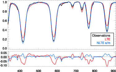
(a)

Figure 11: Top. Selected lines of Na  observed in Procyon (black) and the best fit for the LTE (red) and NLTE(blue) calculations with the parameters in derived in Table 4. Bottom. Difference between observations and the synthetic spectrum in LTE (red) and in NLTE (blue).

Lind et al. (2011) used the MULTI code to calculate LTE and NLTE-s equivalent widths in order to derive Na  abundance corrections for a grid of MARCS model atmospheres. Using their Figure 4, their abundance corrections for Procyon, the Sun and Arcturus are $\sim-0.15,-0.1$ and $-0.2$ respectively while our corrections are $-0.22(9)$, $-0.14(5)$ and $-0.11(5)$ for the three stars. As expected from the departure coefficients in Fig. 7 we find the derived NLTE-s to be the same as the NLTE-m abundances. Figure 11 shows selected lines of Na  in a comparison between observations of Procyon and synthetic spectra in LTE and NLTE. since the NLTE-s and NLTE-m synthetic spectra are indistinguishable, only one of those were plotted. The residuals between observations and the best fit of the synthetic spectra is reduced in NLTE with respect to LTE. We see that for Procyon the best fit in NLTE is 73% better than the best fit in LTE, while for the Sun and Arcturus is 46% and only 5% better respectively.

Our derived solar abundance becomes slightly lower than the value found in CI carbonateous chondrites, after scaling through several well-determined refractory elements (Asplund 2009; Lodders 2019).

6.2 Mg

Osorio et al. (2015) also used the MULTI code for the determination of LTE and NLTE-s Mg  abundances. There is excellent agreement between our absolute LTE and NLTE-s abundances. The NLTE best fit are 10%, 24% and 7% better than the LTE best fit for Procyon, the Sun and Arcturus respectively. As in the case of Na , The effects of the other elements calculated in NLTE are negligible and therefore the NLTE-s and NLTE-m results for Mg  are almost identical.

In this case our derived solar abundance is in better agreement with the meteoritic value, solving a 2$\sigma$ inconsistency shown in previous determinations (Asplund 2009).

6.3 K

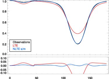
(a)

Figure 12: Top. lines of K  Used in the solar observations (black) compared with the best fit of the LTE (red) and NLTE(blue) calculations with the parameters in derived in Table 4. Bottom. Difference between observations and the synthetic spectrum in LTE (red) and in NLTE (blue).

Reggiani et al. (2019) presented LTE and NLTE abundances for the Sun, Procyon and other stars by fitting the synthetic equivalent widths with the observed ones. The NLTE abundance derived for the Sun is in excellent agreement with ours. In the case of Procyon although the abundance correction is the same (0.68 by Reggiani et al. and 0.66 by us) our LTE and NLTE abundances are higher by 0.19 dex. In Arcturus the LTE and NLTE residuals of the best fit are same: we found an abundance correction of 0.44 dex.

6.4 Ca

The most interesting case is Ca , whose NLTE populations are affected the most by the NLTE populations of the other elements, specifically by Mg . Osorio et al. (2019) presents NLTE-s abundance corrections of Ca  for the three stars studied in this work. In order to make a cleaner comparison, we use the same masks as the ones used in the all-lines calculation in Osorio et al. (2019).

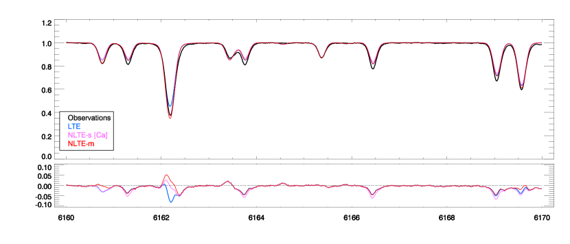
(a)

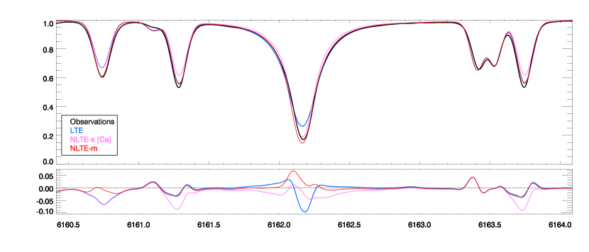
(b)

(c)

Figure 13: Comparison between synthetic spectra and observations of the section around 6162 Å for Procyon (top), the Sun (middle) and Arcturus (bottom) where several Ca  lines can be observed. The black lines represent the observations; blue, pink and red are the synthetic spectra in LTE, NLTE-s[Ca] and NLTE-m respectively. Bellow each spectra the residuals (synthetic-observed) are plotted. The Ca  abundance and V_mac adopted for the LTE, NLTE-s [Ca] and NLTE-m synthetic spectra are [A(Ca), V_mac(Km/s)] = [6.10, 5.1] for Procyon; [6.30, 1.0] for the Sun and [5.99, 3.6] for Arcturus.

For Procyon, Osorio et al. found an abundance correction of $\Delta_{nlte,s}(Ca)=-0.08$ dex while in this work we found $\Delta_{nlte,s}(Ca)=-0.05$ dex although our new LTE Ca  abundance is higher than in Osorio et al.. A possible explanation of the discrepancy is that MULTI calculates line profiles only of the element under study, while SYNSPEC computes synthetic spectra including the contribution from several atomic and molecular species. The effects in Procyon of having a more realistic synthetic spectrum is probably affecting more the derived abundances than in the Sun or in Arcturus. A similar phenomenon happens with K  in Procyon when compared with Reggiani et al. (2019), which also used MULTI in the calculation of the synthetic spectral lines. Our multi-element calculation decreases the derived NLTE-m abundance by 0.03 dex with respect to the NLTE-s results. The top panel of Fig. 13 shows the region around 6165 Å where there are several lines of Ca . It is clear that the core of the 6162 Å line is the weakest in LTE (blue line), then in NLTE-s the core of this line match the observations quite well and the NLTE-m calculations strengthen the core a bit more. If only the 6162 Å line is considered, the fit with observations is better in NLTE-s than in NLTE-m, but by checking the other lines in the window, we note that the other NLTE-s Ca  lines have weaker cores than the LTE profiles and the observations. The NLTE-m spectra have similar line profiles to the LTE for four of the Ca  lines (6161.4, 6163.7, 6166.5 and 6169.1). The 6169.6 Å line has a NLTE-m profile that match better the observations than the LTE and NLTE-s cases. We found that our NLTE-s best fit is 20% and our NLTE-m best fit is 18% better than the LTE best fit.

For the Sun, Osorio et al. (2019) derived an LTE Ca  abundance in agreement to ours, but we found a negligible abundance correction of 0.02 dex while the NLTE-m results show a correction of $-0.05$ dex. The central panel in Fig. 13 shows solar observations and the synthetic spectra in the region around 6162 Å where three Ca  lines are clearly visible. There is also a Na  which has a NLTE line profile in the NLTE-m spectra. The NLTE calculations show that while the core of the 6162 Å line matches better the observations in the NLTE-s and NLTE-m cases than in the LTE one, the wings of the NLTE-s and the other two Ca  lines seen in the figure, suggest that the NLTE-s abundance must increase in order to fit the observations (as the results in Table 4 show). The LTE spectrum is unable to reproduce the core and the wings of the 6162 Å line. While the 6161.3 and 6163.7 Ca  lines are reproduced better in LTE than in NLTE-s. The NLTE-m 6161.3 and 6163.7 Å lines are similar to the LTE lines and with the same abundance the core and the profile of the 6162 Å can be reproduced. The results of this sort of balance shows that our NLTE-s best fit is 20% better than the best fit in LTE and our NLTE-m best fit is 34% better than the best fit in LTE. We should also point out that the NLTE-m Ca  abundance we found is in excellent agreement with the meteoritic value.

Like the other atomic elements studied in this work, Ca  in Arcturus seems to be unaffected by NLTE multi-element effects. The LTE and NLTE-s abundances found by Osorio et al. (2019) agree with ours and the small NLTE corrections are in the same direction ($-0.02$ in this work and $-0.01$  dex in Osorio et al.). As in the work from Osorio et al., the NLTE-s best fit is worse than the LTE best fit (32% in that work and 12% in this work). Will the addition of iron in NLTE-m calculations improve the situation of Ca  in NLTE for Arcturus?, is the NLTE ionisation balance of the important electron donors affecting the total electron populations and therefore the atmospheric structure in Arcturus in a sensible manner? Further investigations will answer those questions.

7 The APOGEE spectral window

The only difference between the analysis of the observations of the Sun and Arcturus in the APOGEE window, and the previous comparison in the optical are the b-b data adopted for SYNSPEC: We adopted the ASPCAP atomic line-list (Shetrone et al., 2015) formatted for SYNSPEC. The molecular b-b data use isotopic ratios suited for the Sun and Arcturus.

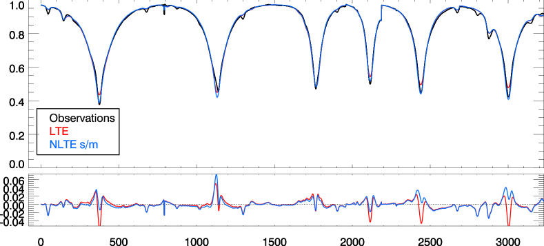
(a)

Figure 14: Comparison between synthetic spectra and centre of disc solar intensity observations of Mg lines in the APOGEE window. The black lines represent the observations; red and blue are the synthetic spectra in LTE and NLTE respectively. Bellow each spectra the residuals (synthetic-observed) are plotted. The Mg  abundance adopted for both synthetic spectra is A(Mg) = 7.55 dex. The label of each line represent the wavelength (in Å).

The solar observations in the $H$-band we adopt correspond to the centre of disc intensity spectrum from Livingston & Wallace (1991). For Na , K  and Ca  there are no significant NLTE effects in the line profiles and therefore the derived abundances in LTE and NLTE are the same. There are only two useful lines of Na  in the $H$-band solar spectrum. The 15992 Å line can be reproduced with A(Na)=6.12 dex, in good agreement with the NLTE Na  solar abundance we derived in the optical. The Na  16388.8 Å line is weaker than the observations using the same abundance, but there are issues to determine the continuum location around this line: it lies in the blue wing of an H-Brackett line ([n_l,n_u]=[4,12] at 1.6398 Å) and has Fe, Ni and Ti blends. The Mg  abundance found using the spectra in the APOGEE region is A(Mg)=7.55 dex, in excellent agreement with our derived abundance from the optical transitions. Like in the optical, we found that the Mg  abundances that correspond to the best fittings in NLTE and LTE are the same, but as seen in Fig. 14 the LTE line profile is unable to reproduce the core of the strong Mg  lines. The observed K  lines in the $H$-band are insensitive to NLTE effects. The derived abundance in the sun is A(K)=5.05 dex, in good agreement as well with our NLTE results for the optical lines. The derived abundance of Ca  found from the 5 lines deemed as useful in the $H$-band is A(Ca)=6.30 dex, in excellent agreement with our NLTE results for the optical. As mentioned before, the LTE and NLTE line profiles for the transitions observed in the $H$-band do not differ significantly, and therefore the derived abundance is the same.

In the case of Arcturus we adopted the observations from Hinkle et al. (1995). For Na , the 15992 Å line has an strong blend with two CN lines and the other visible line (16389 Å) is rather weak but has NLTE effects thus the derived abundances are A(Na_nlte)=5.82 and A(Na_lte)=5.87 dex; both results consistent with our results in the optical. For Mg , abundances of the best fit in LTE and NLTE are A(Mg)=7.55 and 7.40 dex; like in the sun, the core of the strong lines can not be reproduced in LTE. K  has two relatively strong lines at 15170 Å. We found that there are no significant NLTE effects for these two lines and the derived abundance is A(K)=4.80 dex, an intermediate value between the LTE and the NLTE abundances we found in the optical. There are some changes in the Ca  line profiles observed in Arcturus. The derived abundances were A(Ca_nlte)=5.96 and A(Ca_lte)=6.00 dex, both in good agreement with the derived abundance from optical transitions. However, in this case our best fit in NLTE is 12% better than the best fit in LTE. Figure 15 shows the results of the best fit under LTE and NLTE compared with the observations for the selected Ca  lines. The redistribution of the Ca  populations in NLTE shows that for some lines core of the NLTE profile is deeper than the core of the LTE one, while for other lines the opposite is true. Since the NLTE profile is closer to the observations, the line by line analysis will present higher dispersion in the abundances derived in LTE than in NLTE.

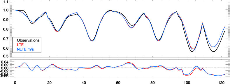
(a)

Figure 15: Comparison of Ca  lines in the apogee window between synthetic spectra and the observations of Arcturus. The black lines represent the observations; red and blue are the best fit synthetic spectra in LTE and NLTE respectively. The lower panel shows the residuals (synthetic-observed).

Regarding the Mg i triplet in the $H$-band, we should stress that the impact of the inability of the LTE calculations to match the observed cores is minimised when the abundance determination is performed fitting line profiles at high resolution, as we are doing here. The cores of the lines span only a few frequencies, the rest of the line profile is reproduced well, and an abundance increase to improve the fitting in the core will necessarily ruin the match in the wings of the line profile. Therefore the best-fitting abundance is fairly insensitive to the NLTE changes in the line core. If the analysis is carried out fitting line profiles at lower resolution, or using equivalent widths, the NLTE abundance corrections will be enhanced. This implies that the abundance corrections expected for these lines in the APOGEE spectra will be significantly augmented compared to our estimates derived for very high-resolution data. We used the NLTE line profile of the 15 748 Å Mg i line as a test case; in both stars the the NLTE cores are stronger than the LTE ones, but in the Sun this line has broad wings and in Arcturus its wings are narrow. We fixed the NLTE abundance and determined the LTE value that minimises the residuals between the two profiles. This experiment was performed at different spectral resolutions, by performing a Gaussian convolution with increasing FWHM in both LTE and NLTE spectra. As seen in Table 5, we find that at increasing resolution the LTE and NLTE profiles become more similar and at the same time the abundance correction increases.

Table 5: NLTE abundance corrections at different resolutions for our test case: The Mg i 15 748 Åline in the Sun and Arcturus

	Sun		Arcturus
FWHM [Å]	$\Delta$A(Mg)	RMSLTE-NLTE	$\Delta$A(Mg)	RMSLTE-NLTE
0.00	-0.02	7.25e-04	-0.04	1.02e-03
0.25	-0.03	1.92e-04	-0.09	6.71e-04
0.50	-0.04	1.12e-04	-0.12	3.14e-04
0.75	-0.05	6.96e-05	-0.14	1.47e-04
1.00	-0.05	4.49e-05	-0.14	7.49e-05
1.50	-0.05	2.23e-05	-0.14	1.92e-05

7.1 Other NLTE work in the APOGEE window

Other NLTE studies in the $H$-band spectra for the atoms studied in this work are the ones from Zhang et al. (2017) for Mg  and Zhou et al. (2019) for Ca .

In Zhang et al. (2017), they adopted for the Sun A(Mg)=7.53 dex and calibrated the oscillator strength of the 15750 Å lines in order to fit the observations. Their figure 2 does not show a deeper NLTE core compared with the LTE line profile, a feature we see in our synthetic spectra (see Fig. 14). We believe the reason for this particular discrepancy is due to the collisional data adopted for the high-lying levels. Hydrogen collisional excitation were ignored for the high-lying levels of Mg i while we used the formula from Kaulakys (1986). Electron collisional ionisation were taken from Seaton (1962), while we used the formula from (Vrinceanu, 2005) and electron collisional excitation for the high-lying levels were taken from van Regemorter (1962), while we used the BSR results of Barklem et al. (2017). The derived NLTE populations of the high-lying levels depend directly on the collisional rates that involve those levels. They also derived LTE and NLTE abundances for Arcturus and found an abundance correction of $\Delta$A(Mg)${}_{nlte-lte}=-0.03$ dex which is consistent with our results.

The work on Ca  presented in Zhou et al. (2019) study both, the optical and the $H$-band spectra. The derived LTE abundances agree with ours for the Sun, but for Arcturus they are $\sim$0.1 dex lower than ours. The reason for this discrepancy can be due to differences in the abundance adopted and the radiative data (they used astrophysical f-values by setting the solar A(Ca)=6.31 dex while we adopted f-values based on Yu & Derevianko 2018, see Table 6).

Table 6: log(gf) values adopted for the Ca i lines visible in the H-band in Zhou et al. (2019) and in this work (taken from Yu & Derevianko, 2018).

$\lambda$ (Å)	Zhou et al. (2019)	This work
16 136.823	$-0.525$	$-0.973$
16 150.763	$-0.215$	$-0.369$
16 155.236	$-0.685$	$-0.624$
16 157.364	$-0.165$	$-0.411$
16 197.075	$0.098$	$-0.016$

For Arcturus they found in the optical an abundance correction of 0.01 dex, which is in excellent agreement with our NLTE-s results. For the $H$-band, Zhou et al. found no abundance correction for Arcturus, while we found -0.04 dex. We think this discrepancy is again due to differences in the collisional data adopted for the high-lying levels. In this work, hydrogen collisional excitation for the high-lying levels of Ca i were ignored, while we used the formula from Kaulakys (1986). For electron collisional ionisation Zhou et al. used the formula from Seaton (1962), while we adopted the formula from Vrinceanu (2005); finally, electron collisional data involving the levels producing the Ca i lines visible in the H-band are from Seaton (1962), while we used an extension of the data presented in Zatsarinny et al. (2019).

8 Conclusions

Traditional (1D and 3D) NLTE calculations in cool stars adopt the trace-element approximation, where all the atmospheric parameters are kept fixed while the populations of a single atomic element are allowed to change. With the aim of removing such approximation, we performed for the first time NLTE radiative transfer calculations in cool stars including several atomic elements simultaneously, still within the trace-element approximation but including the inter-element effects through the background opacities.

Atomic elements in ionisation stages where over-ionisation is an important NLTE mechanism are most likely affected by Mg  NLTE effects. For late-type stars around solar temperature and hotter, there is enough change in the UV flux due to Mg -NLTE effects that it can affect the statistical balance of Ca , but not K  or Na .

Due to the sensitivity of the NLTE results for a particular radiative transition on the collisional data of the levels associated to that transition, special care must be taken when performing NLTE calculations of spectral lines involving high-lying level, for which usually accurate collisional data are missing.

As found in previous studies (Osorio et al., 2019), the best fit for Ca in Arcturus in LTE is better than the best fit for Ca in NLTE-s[Ca] and NLTE-m. Perhaps the calcium NLTE populations in Arcturus are sensitive to other elements than the ones studied here – iron is the obvious candidate. Future calculations expanding the elements to calculate in the NLTE-m mode will help to clarify this issue.

Observations at lower resolution will cause derived LTE abundances to increase due to the inability of the LTE line profiles to match the cores of strong lines (like the Mg i triplet in the $H$-band).

The derived NLTE abundance corrections in the optical and in the H-band differ, but the NLTE abundances derived are consistent between the two spectral regions.

The goal of this effort is to update the synthetic spectral library that will be used by ASPCAP in DR17 which will include inter-element NLTE effects for Na , Mg , K  and Ca  in the analysis of APOGEE spectra.

This work demonstrates that in cool stars inter-element NLTE effects (via background opacities) can have an impact on the derived abundances of the same order as ”traditional” NLTE effects. We expect the inter-element NLTE effects to increase with temperature (due to increased radiative fluxes) and higher surface gravities (due to wider lines). This an step towards full NLTE stellar atmospheric modelling of cool stars. Our next step in this line will be to include more elements that contribute opacity in the next NLTE-m calculations and study its effects on the NLTE results derived for other species.

In Section 4 of Asplund (2005), the author points out the lack of studies regarding the effects of NLTE and 3D on the structure of cool stars, and the possible implications on parameters determined via stellar spectra e.g. $T_{\mathrm{eff}}$ and $\log\,g$ derived from ionisation balance / line broadening. More recently, Asplund et al. (2009, Section 2) points out that even though we have had great progress in the quality and quantity of available atomic data we still require to go beyond LTE in order to attain the desired %1 level of precision in derived solar abundances that are fundamental for the whole astrophysics community. Works regarding the effects of the trace element approach on the NLTE results in cool stars is still an area to explore and this is our first effort on this front.