Non-reciprocal phase transitions

Abstract

Out of equilibrium, the lack of reciprocity is the rule rather than the exception. Non-reciprocal interactions occur, for instance, in networks of neurons Dayan and Abbott (2001); Amir et al. (2016); Krakauer et al. (2017); Montbrió and Pazó (2018); Parisi (1986); Derrida et al. (1987); Sompolinsky and Kanter (1986), directional growth of interfaces Cross and Hohenberg (1993), and synthetic active materials Marchetti et al. (2013); Kotwal et al. (2019); Bricard et al. (2013); Palacci et al. (2013); Geyer et al. (2018); Bain and Bartolo (2019); van Zuiden et al. (2016); Dayan and Abbott (2001); Caussin et al. (2014). While wave propagation in non-reciprocal media has recently been under intense study Fleury et al. (2014); Estep et al. (2014); Coulais et al. (2017); Miri and Alù (2019); Scheibner et al. (2020a); Ghatak et al. (2019); Lee and Thomale (2019); Helbig et al. (2020); Lin et al. (2011); Schindler et al. (2011); Weidemann et al. (2020); Hofmann et al. (2019); Brandenbourger et al. (2019); Bender (2007); Ramos et al. (2020), less is known about the consequences of non-reciprocity on the collective behavior of many-body systems. Here, we show that non-reciprocity leads to time-dependent phases where spontaneously broken symmetries are dynamically restored. The resulting phase transitions are controlled by spectral singularities called exceptional points Kato (1984). We describe the emergence of these phases using insights from bifurcation theory Golubitsky and Stewart (2002); Crawford and Knobloch (1991) and non-Hermitian quantum mechanics Hatano and Nelson (1996); Bender and Boettcher (1998). Our approach captures non-reciprocal generalizations of three archetypal classes of self-organization out of equilibrium: synchronization, flocking and pattern formation. Collective phenomena in these non-reciprocal systems range from active time-(quasi)crystals to exceptional-point enforced pattern-formation and hysteresis. Our work paves the way towards a general theory of critical phenomena in non-reciprocal matter.

Non-reciprocity naturally arises in nonequilibrium many-body systems Nagy et al. (2010); Morin et al. (2015); Ginelli et al. (2015); Yllanes et al. (2017); Durve et al. (2018); Barberis and Peruani (2016); Lavergne et al. (2019); Bonilla and Trenado (2019); Costanzo (2019); Dadhichi et al. (2020); Agudo-Canalejo and Golestanian (2019); Lahiri and Ramaswamy (1997); Lahiri et al. (2000); Chajwa et al. (2020); Gupta et al. (2020); Soto and Golestanian (2014); Ivlev et al. (2015); Kryuchkov et al. (2018); Saha et al. (2019); Maitra et al. (2020); Uchida and Golestanian (2010); Hanai et al. (2019); Hanai and Littlewood (2020); Metelmann and Clerk (2015) ranging from inhibitory and excitatory neurons Dayan and Abbott (2001); Amir et al. (2016); Krakauer et al. (2017); Montbrió and Pazó (2018); Parisi (1986); Derrida et al. (1987); Sompolinsky and Kanter (1986) to conformist and contrarian members of social groups Hong and Strogatz (2011a, b); Pluchino et al. (2005). Our goal is to explore how non-reciprocity affects phase transitions. To do so, we consider multiple species or fields (interacting non-reciprocally with one another) modeled by a vector order parameter $\vec{v}_{a}(t,\vec{x})$ for each species $a$. These can encode, for instance, the average velocities of self-propelled particles, the average phases of coupled oscillators such as biological clocks or firing neurons, or the amplitude and position of a periodic pattern (Fig. 1a-d). The order parameters $\vec{v}_{a}(t,\vec{x})$ could either be distinct fields, or different harmonics of the same physical field such as in directional interface growth experiments Malomed and Tribelsky (1984); Coullet et al. (1989); Flesselles et al. (1991); Pan and de Bruyn (1994), see Fig. 1e-f.

All of these systems are described by the evolution equation

$$\partial_{t}\vec{v}_{a}=\mathbb{A}_{ab}\,\vec{v}_{b}+\mathbb{B}_{abcd}\,({\vec{v}_{b}\cdot\vec{v}_{c}})\,\vec{v}_{d}+\mathcal{O}(\nabla)$$ (1)

where summation over repeated indices is implied. Equation (1) is (up to third order in $\vec{v}_{a}$) the most general dynamical system invariant under rotations. In flocking, rotational symmetry naturally arises from the isotropy of space, while in synchronization and pattern formation it emerges from the underlying time or space translation invariance. Different symmetries or other representations of rotations can be similarly enforced Golubitsky and Stewart (2002) leading to variants of Eq. (1), see Methods and SI Sec. VIII. The quantities $\mathbb{A}_{ab}$ and $\mathbb{B}_{abcd}$ are arrays of parameters that couple the different species of fields. As we shall see, they are also matrices operating on the vectors $\vec{v}_{a}$ that reduce to the identity for full rotation symmetry, but have more complicated forms when parity (mirror reflection) is broken.

While our ultimate goal is to model spatially extended systems, we have temporarily omitted in Eq. (1) terms with spatial derivatives and only retained nonlinearities essential to discuss transitions between distinct non-equilibrium steady-states. Here, we allow the macroscopic coefficients to be asymmetric, e.g. $\mathbb{A}_{ab}\neq\mathbb{A}_{ba}$. In the Landau theory of equilibrium phase transitions, these coefficients would be fully symmetric because the dynamics of the order parameter $\partial_{t}\vec{v}_{a}=-\partial_{\vec{v}_{a}}F$ is derived from a free energy $F$. Removing this symmetry constraint allows to extend the theory of critical phenomena Hohenberg and Halperin (1977) to fields with non-reciprocal interactions.

Dynamical systems described by Eq. (1) arise in various forms of non-reciprocal matter. Consider, for instance, a collection of coupled oscillators described by the Kuramoto model Kuramoto (1984); Acebrón et al. (2005)

$$\partial_{t}\theta_{m}=\omega_{m}+\sum_{n}J_{mn}\sin(\theta_{n}-\theta_{m})+\eta(t).$$ (2)

The metronome or neuron labeled by $m$ in Eq. (2) ticks or fires when its phase $\theta_{m}(t)$ crosses a fixed value (say zero). The oscillator $m$ has a natural frequency $\omega_{m}$ and is coupled to the other oscillators by $J_{mn}$. In the Kuramoto model, the oscillators are typically all coupled and the random noise $\eta(t)$ is usually ignored. Equation (2) with $\omega_{m}=0$ and with random noise also captures the Vicsek model of flocking Vicsek et al. (1995); Toner and Tu (1995), provided that the oscillators are replaced by self-propelled particles moving at constant speed $v_{0}$ in the plane in the direction $\theta_{m}$. Their positions $\vec{r}_{m}$ then follow the equation

$$\partial_{t}\vec{r}_{m}=v_{0}\,\begin{pmatrix}\cos\theta_{m}\\ \sin\theta_{m}\end{pmatrix}.$$ (3)

The couplings $J_{mn}$ are short-ranged and depend on $\vec{r}_{m}$. In both models, the agent $m$ tries to align (be in phase) with the agent $n$ when $J_{mn}$ is positive, and to antialign with it when $J_{mn}$ is negative.

Above a critical coupling, both models exhibit a phase transition from incoherent motion (incoherent oscillations) to flocking (synchronization) heralded by a non-vanishing order parameter $\vec{v}_{a}$ (Fig. 1a,c). We show in the Methods and SI Sec. I that coarse-graining these microscopic models leads to an evolution equation of the form of Eq. (1), with the addition of rotationally invariant terms with spatial derivatives [see Eqs. (11) and (30)]. As expected, the coefficients of the order parameter equations become asymmetric when the interaction is non-reciprocal (i.e., when $J_{mn}\neq J_{nm}$), see also Refs. Daido (1992); Sakaguchi and Kuramoto (1986); Pal et al. (2017); Hong and Strogatz (2011a, b); Martens et al. (2009); Bonilla et al. (1998); Uchida and Golestanian (2010); Hong and Strogatz (2012); Ott and Antonsen (2008); Abrams et al. (2008); Pikovsky and Rosenblum (2008); Choe et al. (2016); Gallego et al. (2017); Bonilla and Trenado (2019); O’Keeffe et al. (2017); Levis et al. (2019); Das et al. (2002, 2004); Matheny et al. (2019) for situations in which this can occur. Equation (1), viewed as an amplitude equation, also describes non-reciprocal pattern formation far from equilibrium Cross and Hohenberg (1993) (Fig. 1e). For example, the non-reciprocal Swift-Hohenberg model Swift and Hohenberg (1977)

$$\partial_{t}u_{a}=r_{ab}u_{b}-(1+\nabla^{2})^{2}u_{a}-gu_{a}^{3}$$ (4)

with $r_{ab}\neq r_{ba}$ reduces to Eq. (1) by letting $u_{a}(x)=A_{a}(x)\text{e}^{\text{i}kx}+\text{c.c.}$, where $k$ is a wavevector and the complex amplitude is decomposed as $A_{a}\equiv v_{a}^{x}+\text{i}v_{a}^{y}$ (see Methods).

Let us start with only two species A and B and consider models where parity is not explicitly broken. When the inter-species interactions are reciprocal, we find (besides a disordered phase) two static phases where the order parameters $\vec{v}_{A}$ and $\vec{v}_{B}$ (red and blue arrows in Fig. 1g-i) are either aligned or antialigned, in analogy with (anti)ferromagnetism. When the inter-species interactions are non-reciprocal, the macroscopic coefficients in Eq. (1) can become asymmetric and we find a time-dependent chiral phase with no equilibrium analogue that emerges between the static phases (Fig. 1g-h). In this intermediate chiral phase, parity is spontaneously broken: $\vec{v}_{A}$ and $\vec{v}_{B}$ rotate either clockwise or counterclockwise at a constant speed $\Omega_{\text{ss}}$, while keeping a fixed relative angle. We stress that this rotation of the order parameters is different from the precession of spins in a magnetic field, that can be simply captured with a Hamiltonian.

Figure 1a-f illustrates the aligned and chiral phases in synchronization, flocking and pattern formation. Panels e-f show a manifestation of the aligned to chiral transition in viscous fingering experiments Pan and de Bruyn (1994); Rabaud et al. (1990); Cummins et al. (1993); Bellon et al. (1998), see Methods for a detailed treatment. We have identified additional examples in naturally occurring phenomena ranging from directional solidification of liquid-crystals Simon et al. (1988); Flesselles et al. (1991); Melo and Oswald (1990); Oswald et al. (1987) and growth of lamellar eutectics Faivre et al. (1989); Faivre and Mergy (1992); Kassner and Misbah (1990); Ginibre et al. (1997) to overflowing fountains Counillon et al. (1997); Brunet et al. (2001). Unlike the examples in panels a-d where two species are present, here the non-reciprocal (asymmetric) couplings in the amplitude equations occur between two different harmonics $A$ and $B$ of the same physical field, see Methods.

Intuitively, the chiral phase is caused by the frustration experienced by species with opposite goals. For concreteness, consider two populations of agents $A$ and $B$ where $A$ want to align with $B$ but $B$ want to antialign with $A$. As the agents are never satisfied, they start running in circles. This dynamical frustration results macroscopically in a constant “chase and runaway” motion of the order parameters ${\vec{v}}_{a}$: this is the chiral phase.

Less intuitively, but crucially, the chiral phase hinges on a subtle interplay between noise and many-body effects. Let us first consider an exactly solvable example: the Kuramoto model in Eq. (2) with noise set to zero and identical frequencies within each species. In this case, the dynamics of the two populations can be mapped to a system with only two agents (SI Sec. VI). Unless the interaction is precisely non-reciprocal (i.e., $J_{AB}\equiv-J_{BA}$), this system always converges to a static phase as the two effective agents will eventually align or antialign when one catches up with the other (SI Sec. V). However, the presence of microscopic noise or frequency disorder in Eq. (2) constantly resets and restarts the chase and runaway motion of A/B pairs. In a many-body system, the noise-activated motions of individual agents become macroscopically correlated through their interactions and the chiral motion is stabilized. We verified this numerically by computing the standard deviations of the order parameters in the chiral phase that decrease as $1/\sqrt{N}$ with the number of agents $N$, see SI Fig. S6. While not exactly solvable, the flocking model exhibits the same phenomenon; noise enlarges the size of the region in which time-dependent phases exist (compare Fig. 2b and Fig. 2c). This is reminiscent of so-called order-by-disorder transitions in frustrated many-body systems Villain et al. (1980); Daido (1992).

To elucidate the many-body character of the aligned to chiral transitions, it is instructive to contrast them to analogous phenomena occurring for only two coupled nonlinear ring-resonators in PT-symmetric lasers Hassan et al. (2015); Miri and Alù (2019); Liertzer et al. (2012); Lumer et al. (2013) (see SI Sec. IX). In this case, the state of the system randomly switches between clockwise and counterclockwise under the effect of noise Hassan et al. (2015), destroying the chiral phase. This noise-activated process would also occur in any of the systems we consider if too few constituents (e.g. agents or resonators) were present. We can model it by adding a hydrodynamic noise to the right-hand side of Eq. (1), see SI Sec. VII. The average time $\tau$ between successive chirality flips follows an Arrhenius law $\tau=\tau_{0}\exp(\Delta/\sigma^{2})$ where $\Delta$ is the height of the effective barrier between the clockwise and counterclockwise states, $\sigma$ is the standard deviation of the hydrodynamic noise, and $\tau_{0}$ is a constant determined from microscopics. When a large number $N$ of constituents is considered, the central limit theorem suggests that $\sigma\sim\sigma_{0}/\sqrt{N}$ ($\sigma_{0}$ is the strength of the noise acting on a single element), consistent with our numerical observations (see SI Secs. V-VII). As a result, the time $\tau$ between chirality flips grows exponentially with $N$: the chiral phase is salvaged by many-body effects. In optics, this scenario could be realized by implementing non-reciprocal couplings Miri and Alù (2019) in photonic networks of many coupled lasers Nixon et al. (2013); Pal et al. (2017); Mahler et al. (2020); Parto et al. (2020); Ramos et al. (2020); Honari-Latifpour and Miri (2020a, b); Acebrón et al. (2005).

Unlike the familiar paramagnet to ferromagnet transition, the aligned to chiral transition (and the chiral phase itself) cannot occur in thermodynamic equilibrium. Here, we develop a general approach to describe this class of time-dependent phases and transitions unique to non-reciprocal matter. Our starting point is a general principle that applies both in and out of equilibrium: phases of a many-body system can be identified from the steady-states of the corresponding dynamical system (such as Eq. (1)). Phase transitions then occur when one steady-state becomes unstable, i.e. when perturbations around it are no longer damped. We therefore linearize Eq. (1), by separating the order parameters $\vec{V}\equiv(\vec{v}_{A},\vec{v}_{B},\dots)$ into steady-state components $\vec{V}_{\text{ss}}$ and fluctuations $\delta\vec{V}$ around them. We obtain the equation

$$\partial_{t}\delta\vec{V}=L\;\delta\vec{V}.$$ (5)

Crucial to our approach is the following fact: non-reciprocity implies that the linear operator $L$ can be non-Hermitian. Consider first a conservative system deriving from a free energy $F$. In this case, we would have $L_{ab}=-\partial_{\vec{v}_{b}}\partial_{\vec{v}_{a}}F=L_{ba}$. This implies that $L$ would be Hermitian, i.e. $L_{ab}=L_{ba}$, as it is real valued. In contrast, a non-reciprocal system cannot be described by a free energy. As a result, $L$ can be and generally is non-Hermitian, i.e. $L_{ab}\neq L_{ba}$.

The linear operator $L$ determines the nature of phase transitions in non-reciprocal matter through the dynamics of fluctuations. The $2M$ eigenvectors of $L\equiv L(\vec{V}_{\text{ss}})$ (for $M$ species) describe the time evolution of fluctuations around the steady-state. They do not have to be orthogonal because $L$ is not Hermitian. The corresponding eigenvalues $s_{i}=\sigma_{i}+\text{i}\omega_{i}$ can be decomposed in growth rates $\sigma_{i}$ and frequencies $\omega_{i}$ where $i=1,\dots,2M$. Here, one of the eigenmodes of $L$ always has a vanishing eigenvalue $s=0$, because it corresponds to a global rotation of the $\vec{v}_{a}$ (i.e., the Goldstone mode of broken rotation invariance), green line in Fig. 1h. In the static (anti)aligned phase, the other modes are always damped ($\sigma_{i}<0$). The aligned-to-chiral phase transitions occur when the damped mode with the growth rate $\sigma_{i}$ closest to zero (orange line in Fig. 1h) coalesces with the Goldstone mode (green line) at special points labeled in red.

This coalescence of two eigenmodes is known as an exceptional point (EP) Kato (1984). In addition to having the same eigenvalues (that crucially vanish in our case), the two eigenmodes become parallel at the exceptional point Hanai and Littlewood (2020). In a many-body system, such a mode coalescence defines a class of phase transitions that we dub exceptional transitions. As an illustration, imagine a ball constantly kicked by noise at the bottom of a potential shaped as a Mexican hat. In this simplified picture, the ball represents the order parameter of a many-body system. In a reciprocal system, the ball rolls back to the bottom when perturbed in the uphill direction. In a non-reciprocal system, there are non-conservative forces in addition to the potential energy landscape, that lead to transverse responses. When you kick the ball in the uphill direction, it also moves perpendicular to it along the bottom of the potential, but not vice-versa. This non-reciprocal response is described mathematically by the non-orthogonality of the eigenmodes of $L$. At the exceptional point, the ball moves along the bottom of the potential irrespective of whether it is kicked along or perpendicular to it. This corresponds to the coalescence between the Goldstone mode and the damped mode with growth rate $\sigma$ closest to zero. After the exceptional transition, the ball starts running along the bottom of the potential by itself, at a speed set by the now positive growth rate $\sigma$ (Fig. 1h).

More generally, exceptional transitions can be viewed as the dynamical restoration of a spontaneously broken continuous symmetry: the Goldstone mode is actuated by the noise, and after the transition the system runs along the manifold of degenerate ground states. Figure 1i provides an almost mechanical picture of how non-reciprocal interactions lead to an exceptional point and to the onset of the chiral phase. From the point of view of non-Hermitian quantum mechanics Hatano and Nelson (1996); Bender and Boettcher (1998), these transitions are manifestations of the spontaneous PT symmetry breaking (see Methods). From the point of view of dynamical systems, they are instances of Bogdanov-Takens bifurcations Kuznetsov (2004), with the peculiarity that one of the modes involved is a Goldstone mode (see Methods).

As a concrete example, let us consider the continuum theory of non-reciprocal flocking [Methods Eq. (11)]. Analogous treatments of synchronization and pattern formation are detailed in Methods. Figure 2a-c shows the key result of our analysis based on Eq. (11): the phase diagrams as a function of the reciprocal and non-reciprocal parts of the rescaled inter-species interactions $j_{\pm}=[j_{AB}\pm j_{BA}]/2$ respectively (see SI Sec. II). These phase diagrams exhibit a disordered phase (gray), an aligned phase (blue), an antialigned phase (red), and a chiral phase (purple, see also Fig. 2d). In the SI Sec. III, we prove that these phases are linearly stable against velocity fluctuations in the hydrodynamic theory over large ranges of parameters. This theory further predicts that the phase boundary between the chiral phase and the (anti)aligned phase is marked by exceptional points (red lines in Fig. 2c).

The chiral phase is not the only time-dependent phase induced by non-reciprocity. We have also identified a swap phase (green region in Fig. 2b-c), where $\vec{v}_{A}$ and $\vec{v}_{B}$ oscillate between two values along a fixed direction. In contrast with the chiral phase where a continuous symmetry is restored on average, the swap phase dynamically restores a discrete symmetry through the loss of time-translation invariance. We also predict and observe a mixed chiral+swap phase, where both swap and chiral motions occur at the same time (dark green region). The dynamical nature of these phases is illustrated in Fig. 2d-e and SI Movie 2. All these phases break time translation invariance, in a way reminiscent of time crystals Shapere and Wilczek (2012); Wilczek (2012); Khemani et al. (2019); Yao and Nayak (2018); Prigogine and Lefever (1968); Winfree (2001) and quasicrystals Giergiel et al. (2018); Autti et al. (2018), see Fig. 2f-g. The existence of all the phases found in non-reciprocal flocking follows from general symmetry principles Golubitsky and Stewart (2002). Hence, they transcend specific models. We also observe them in our non-reciprocal synchronization (Extended Data Fig. 4) and pattern formation models (Extended Data Fig. 7), see Methods.

We now show that exceptional transitions must necessarily be accompanied by pattern-forming instabilities when the non-reciprocally interacting constituents are moving, i.e. when there is a steady-state flow $\vec{v}_{\text{ss}}$. Figure 3a shows that pattern formation occurs around the critical lines marking the mean-field phase transition (bright red and blue regions). This phenomenon can be captured by the following model

$$\partial_{t}\,\delta\vec{V}=\big{[}L_{\text{EP}}+M(\vec{v}_{\text{ss}}\cdot\nabla)+D\,\nabla^{2}\big{]}\delta\vec{V}.$$ (6)

Equation (6) is a minimal extension of Eq. (5) valid near the exceptional transition where $L_{\text{EP}}$ is the singular matrix accounting for the presence of the exceptional point. It contains an additional convective term in the linearized matrix form $M(\vec{v}_{\text{ss}}\cdot\nabla)$ that mixes the two species $A$ and $B$ as well as a diffusive term $D\,\nabla^{2}$. Since the eigenvalues of a perturbed exceptional point typically diverge as a square root of the perturbation Kato (1984), the momentum space complex growth rate behaves as $s_{\pm}(k)\simeq\pm\text{i}\sqrt{\text{i}v_{\text{ss}}\,k}$ at small wavevector $k$, and as $-D\,k^{2}$ at large $k$. This leads to a positive maximum in the growth rate, corresponding to a linear instability at finite momentum (Fig. 3b-c).

Figure 3d-f and SI Movie 4 provide glimpses into the non-linear regime of pattern formation in which vortices and antivortices continuously unbind and annihilate. The density of topological defects is different in $\vec{v}_{A}$ and $\vec{v}_{B}$ because each density decreases with the self-propulsion speed of the respective species (Fig. 3d-e). While the system does not coarsen towards an ordered state, there is a clear precursor of the chiral phase within its chaotic dynamics: the angular distribution of the order parameters plotted in Fig. 3f is approximately periodic.

We have seen that parity is spontaneously broken in the chiral phase. It is also natural to consider systems in which parity is explicitly broken. Concrete examples include: (i) the Kuramoto model Eq. (2) with nonvanishing natural frequencies (ii) the Vicsek model Eqs. (2–3) with external torques or (iii) the Swift-Hohenberg model Eq. (4) with broken up-down ($u\to-u$) symmetry. All these systems still fit in the framework of Eq. (1), provided that the matrices $\mathbb{A}^{\mu\nu}_{ab}$ and $\mathbb{B}^{\mu\nu}_{abcd}$ acting on $\vec{v}_{a}^{\,\nu}(t,x)$ are appropriately chosen ($\mu$ and $\nu$ denote the vector components). By imposing the rotational symmetry constraint, we can fully determine the form of these matrices: $\mathbb{A}_{ab}^{\mu\nu}=\alpha_{ab}\,\delta^{\mu\nu}+{\alpha}^{\star}_{ab}\,\epsilon^{\mu\nu}$ and $\mathbb{B}_{abcd}^{\mu\nu}=\beta_{abcd}\delta^{\mu\nu}+{\beta}^{\star}_{abcd}\,\epsilon^{\mu\nu}$. Here, $\delta^{\mu\nu}$ is the identity and $\epsilon^{\mu\nu}$ is an antisymmetric matrix that rotates the vectors by $90\mathrm{°}$. Using this decomposition, we can distinguish (I) parity symmetric systems in which $\alpha^{\star}$ and $\beta^{\star}$ vanish and (II) systems in which parity is explicitly broken, in which $\alpha^{\star}$ and $\beta^{\star}$ can be nonzero. The classes I and II correspond to the symmetry groups of general rotations $O(2)$ and proper rotations $SO(2)$, respectively.

In the language of non-Hermitian quantum mechanics Bender and Boettcher (1998); Mostafazadeh (2002a); Miri and Alù (2019), class I systems exhibit PT-symmetry, which may be spontaneously broken in the chiral phase. In this case, reaching an exceptional transition requires tuning only one parameter (the transitions have codimension one, see e.g. Fig. 2 where they are lines in a 2D phase diagram). In class II, on the other hand, PT symmetry is explicitly broken: as a result, the equivalent of the aligned and antialigned phases become time-dependent, and reaching an exceptional point requires tuning two parameters (the exceptional points have codimension two, see e.g. Extended Data Fig. 6 and Fig. 4 where they are isolated points in 2D).

In the Methods, we present a detailed analysis of the non-reciprocal Kuramoto model (2) with non-vanishing $\omega_{m}$ that explicitly breaks parity. The combination of non-reciprocity and explicit PT-symmetry breaking leads to hysteresis and discontinuous transitions between (i) regions where the clockwise and counterclockwise states coexist and (ii) regions where only one state exists (Extended Data Fig. 6). These results reveal a remarkable similarity between non-reciprocal synchronization and driven Bose-Einstein condensates Hanai et al. (2019); Hanai and Littlewood (2020).

We conclude with a visual procedure to extend our approach to other systems (Figure 4). The key ingredients are (i) macroscopic non-reciprocity (manifested in the asymmetry of macroscopic coefficients) and (ii) a spontaneously broken continuous symmetry. Although we have focused mostly on systems with circular symmetry $O(2)$, exceptional transitions could occur for any continuous group, see SI Sec. VIII for an extension to spherical symmetry $O(3)$ relevant to three-dimensional vector order parameters such as in 3D flocks. Our analysis was illustrated with vector order parameters whose evolution is not the expression of a conservation law. This paradigmatic case is known as “model A” in the Hohenberg-Halperin classification of dynamical critical phenomena Hohenberg and Halperin (1977) but the same approach applies also to other order parameters and classes, see Ref. Scheibner et al. (2020a) for a non-reciprocal active elasticity that conserves linear momentum and Refs. You et al. (2020); Saha et al. (2020) for non-reciprocal models of phase separation that conserve mass (both illustrate “model B” in Ref. Hohenberg and Halperin (1977)).

Our work lays the foundation for a general theory of critical phenomena in non-reciprocal matter from driven quantum condensates to biological and artificial neural networks. These systems are marked by the interplay between the non-reciprocal enhancement of the fluctuations and the rigidity bestowed by many-body effects. Our field-theoretical approach inspired by non-Hermitian quantum mechanics captures these effects and builds new bridges between many-body physics and bifurcation theory.

Acknowledgments. We thank Andrea Alù, Denis Bartolo, Demetrios Christodoulides, Aashish Clerk, Alexander Edelman, Alexey Galda, Ming Han, Kabir Husain, Tsampikos Kottos, Zhiyue Lu, M. Cristina Marchetti, Mohammad-Ali Miri, Benjamin Roussel, Colin Scheibner, David Schuster, Jonathan Simon, and Benny van Zuiden. MF acknowledges support from a MRSEC-funded Kadanoff-Rice fellowship (DMR-2011854) and the Simons foundation. RH was supported by a Grand-in-Aid for JSPS fellows (Grant No. 17J01238). VV was supported by the Complex Dynamics and Systems Program of the Army Research Office under grant no. W911NF-19-1-0268 and the Simons foundation. This work was partially supported by the University of Chicago Materials Research Science and Engineering Center, which is funded by National Science Foundation under award number DMR-2011854. This work was completed in part with resources provided by the University of Chicago’s Research Computing Center. Some of us benefited from participation in the KITP program on Symmetry, Thermodynamics and Topology in Active Matter supported by grant no. NSF PHY-1748958.

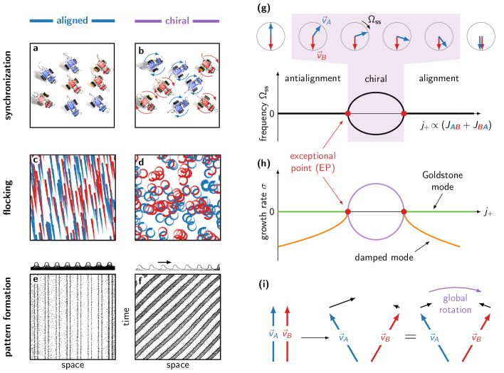
Fig. 1: Exceptional transitions from non-reciprocity and continuous symmetries. Non-reciprocal interactions between two species $A$ and $B$ ($J_{AB}\neq J_{BA}$) induce a phase transition from static alignment to a chiral motion that spontaneously breaks parity. (a-b) Non-reciprocal synchronization. The oscillators represented by robots (programmed as non-reciprocal spins) spontaneously rotate either clockwise or counterclockwise, despite having no average natural frequency, i.e. $\omega_{m}=0$ in Eq. (2). (See SI Movie 3 for a demonstration.) (c-d) Non-reciprocal flocking. The oscillators are replaced by self-propelled particles. They run in circles, either clockwise or counterclockwise, despite the absence of any external torque. See Fig. 2 for details and SI Movie 1 for movies of the simulations. (e-f) Non-reciprocal pattern formation. A one-dimensional pattern starts traveling, either to the left or to the right, see Methods for details. The figure represents an experimental observation of viscous fingering at an oil-air interface adapted with permission from Ref. Pan and de Bruyn (1994) (Copyright 1994 by the American Physical Society). In this case, the species correspond to different harmonics of the same field. (g) Schematic bifurcation diagram of the exceptional transition showing the frequency of the steady-state $\Omega_{\text{ss}}$. Between the static phases with alignment and antialignment (in which $\Omega_{\text{ss}}=0$), we find an intermediate chiral phase that spontaneously breaks parity. Two equivalent steady-states (clockwise and counterclockwise, corresponding to opposite values of $\Omega_{\text{ss}}$) are present in this time-dependent phase, which can be seen as a manifestation of spontaneous PT-symmetry breaking. The chiral phase continuously interpolates between the antialigned and aligned phases, both through $|\Omega_{\text{ss}}|$ and through the angle between the order parameters $\vec{v}_{A}$ and $\vec{v}_{B}$. (h) The transition between (anti)aligned and chiral phases occurs through the coalescence of a damped mode (orange) and a Goldstone mode (green) at an exceptional point (EP, marked by a red circle). (i) Non-reciprocity leads to an exceptional point. In a reciprocal system, rotating the order parameter $\vec{v}_{A}$ has the same effect on $\vec{v}_{B}$ as rotating $\vec{v}_{B}$ would have on $\vec{v}_{A}$. By definition, this is not the case in non-reciprocal systems. Hence, a purely antisymmetric perturbation (for which the velocities $\vec{v}_{A}$ and $\vec{v}_{B}$ are rotated by equal amounts in opposite directions) does not generate a purely antisymmetric response: $\vec{v}_{A}$ is rotated back by a greater amount than $\vec{v}_{B}$ (black arrows in middle panel). This response is equivalent to pushing back $\vec{v}_{A}$ and $\vec{v}_{B}$ towards each other by equal amounts (black arrows in right panel), plus applying a global rotation (purple arrow). The purely symmetric perturbation (solid-body rotation) is a Goldstone mode, so it does not generate any response. As the non-reciprocal coupling increases, it reaches a critical value where all perturbations result in a global rotation of $\vec{v}_{A}$ and $\vec{v}_{B}$. This corresponds to an exceptional point and marks the onset of the chiral phase.

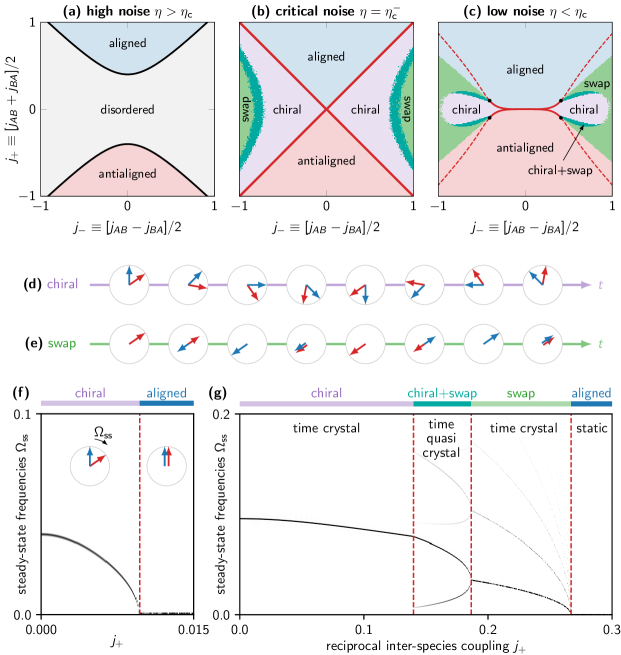
Fig. 2: Many-body exceptional points and active time (quasi)crystals. (a-c) Slices of the phase diagram of the non-reciprocal flocking model Eq. (11) for different values of the noise strength $\eta$. The parameters $j_{ab}$ (entering $\alpha_{ab}$ and $\beta_{abcd}$ in Eq. (1)) are coarse-grained versions of the microscopic couplings $J_{ab}$. The red (resp. black) lines correspond to the analytically-determined phase transition lines from the (anti)aligned phase to the chiral (resp. disordered) phase. The red lines correspond to lines of exceptional points. In (b) and (c), the analytical prediction for the (anti)aligned/chiral transition is in excellent agreement with the numerical phase diagram up to tetracritical points marked by black dots where new phases emerge (see SI Sec. II). (d) Schematic representation of one period of the chiral phase: $\vec{v}_{A}$ and $\vec{v}_{B}$ rotate in block at a constant angular velocity $\Omega_{\text{ss}}$, see SI Movie 2. (e) Schematic representation of one period of the swap phase: $\vec{v}_{A}$ and $\vec{v}_{B}$ oscillate along a fixed direction, see SI Movie 2. (f,g) Plot of the frequencies present in the steady-state solution as a function of $j_{+}$, (f) for $j_{-}=$-0.6$$ and (g) for $j_{-}=$-0.25$$. In the chiral phase, a single frequency is present in the spectrum (at each point), which corresponds to the solid-body rotation. In the swap phase, a single frequency accompanied by harmonics are present. In contrast, in the mixed chiral/swap phase, two independent frequencies are present (with their harmonics). These frequencies are not harmonics of each other, leading to a quasiperiodic phase. The aligned phase is static ($\Omega_{\text{ss}}=0$). Similar plots would be observed with the antialigned phase. In (g), a direct transition between aligned and chiral phases is observed. The phase diagrams are determined by solving Methods Eq. (11) numerically from random initial conditions, with $\rho_{A}=\rho_{B}=$1$$, $j_{AA}=j_{BB}=$1$$, and (a) $\eta/\eta_{\text{c}}=$1.5$$, (b) $\eta/\eta_{\text{c}}=$0.99$$, (c) $\eta/\eta_{\text{c}}=$0.5$$. The parameters in (f,g) are the same as in (c).

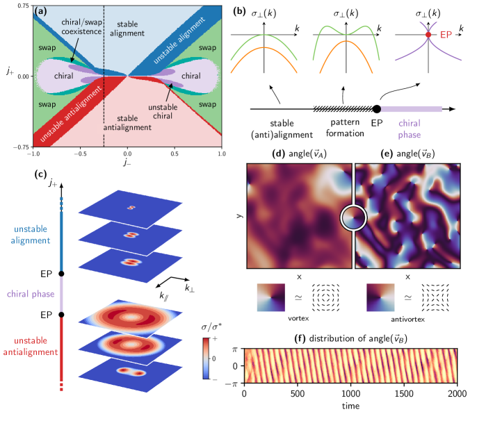
Fig. 3: Stability of spatially extended systems: exceptional-point enforced pattern formation. The combination of convective terms with exceptional point at the (anti)aligned to chiral transitions gives rise to pattern formation near the transition lines. (a) Numerical phase diagram including the linear stability analysis of the (anti)aligned and chiral phases in the non-reciprocal Toner-Tu model (the stability of the swap and chiral+swap phases is not analyzed). (b) Mechanism of exceptional transition and of exceptional-point enforced pattern formation. The coalescence of the Goldstone mode with a damped mode lead to instabilities at finite momentum. The growth rate of transverse perturbations $\sigma_{\bot}(k)$ becomes positive, and has a maximum $\sigma^{*}$ at a finite wavevector $k^{*}$. (c) Plot of the normalized growth rate $\sigma(k)/\sigma^{*}$ as a function of wavevector, for different values of $j_{+}$ at fixed $j_{-}$ [along the dashed line in (a)]. (c-f) Fully non-linear simulation of the pattern formation in the unstable aligned regime. We show snapshots of the angle with a fixed direction (d-e) of the order parameters $\vec{v}_{A}$ and $\vec{v}_{B}$ (see SI Movie 4 of the time evolution). Note the existence of numerous topological defects (vortices and antivortices) in the order parameters. In (f), we show the evolution in time of the histogram of the angle between $\vec{v}_{A}$ and a fixed direction (the corresponding plot for $\vec{v}_{B}$ has identical features). An approximate periodicity emerges amidst the spatio-temporal chaos, ushering in the chiral phase. We have used the same parameters as in Fig. 2 with $\eta/\eta_{\text{c}}=$0.5$$. In (a-b), $v^{0}_{A}=$0.06$$ and $v^{0}_{B}=$0.01$$. The simulations in (c-g) are performed on a $2L\times 2L$ box with periodic boundary conditions, and $L=$0.32$$, $j_{+}=$0.1$$, $j_{-}=$0.2$$, $v^{0}_{A}=$0.06$$ and $v^{0}_{B}=$0.01$$ (see Methods for details on the simulation).

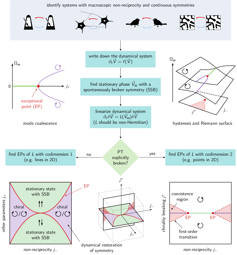
Fig. 4: A visual procedure to identify and analyze exceptional transitions. We start by identifying a system with (i) non-reciprocal interactions between two or more components and (ii) a continuous symmetry that can be spontaneously broken. A dynamical system describes the evolution of the relevant order parameter $V$ (an effective hydrodynamic theory), obtained either purely by symmetry considerations, or from more microscopic considerations. We then look for a time-independent (stationary) steady-state $V_{\text{ss}}$ in which a continuous symmetry is spontaneously broken (SSB, green regions). The dynamical system is then linearized above this time-independent steady-state. Because of the spontaneously broken symmetry, the corresponding linear operator (Jacobian matrix) $L(V)$ always has a vanishing eigenvalue. The exceptional points (EP, red points and continuous red lines) of $L(V)$ with zero eigenvalue correspond to exceptional transitions. The parameters of the system are separated in two classes: (I) those who do not explicitly break parity, collectively labeled by $j$, and (II) those who explicitly break parity, labeled by $j^{\star}$. We further split the parameter set $j$ into two subclasses, (a) $j_{-}$ for parameters encoding the non-reciprocity and (b) $j_{+}$ for the others. When $j^{\star}=0$ (left panel), the EP have codimension 1 (they form lines in a 2D parameter space). At the exceptional transition, the Goldstone mode collides with a damped mode. This leads to a spontaneous dynamical restoration of symmetry (at the price of losing time-translation invariance) in which the Goldstone mode is actuated by the fluctuations. In the corresponding chiral phase (in purple), the space of equivalent steady-states (corresponding to the broken symmetry) is traveled in a direction (clockwise or counterclockwise) chosen at random. When $j^{\star}\neq 0$, this mechanism competes with an explicit rotation of the order parameter set by $j^{\star}$. This leads to extended regions (in light red) starting at the EP (red point, now of codimension 2) in which the (counter)clockwise states coexist, marked by first-order transitions and accompanied by hysteresis: the complex frequencies of the (stable) equilibrium states are organized on a Riemann surface (see Extended Data Fig. 6 for a numerically computed version in the non-reciprocal Kuramoto model).

METHODS

I Non-reciprocity out of equilibrium

In this section, we discuss the relations between non-reciprocity, the non-Hermitian (non-normal) character of the Jacobian of a dynamical system, which allows it to exhibit an exceptional point, and the non-equilibrium character of the system.

A dynamical system

$$\partial_{t}X=f(X)$$ (7)

is said to be conservative when it derives from some potential $F$ (e.g., a free-energy), such that $f_{a}(X)=\partial_{X_{a}}F$. (Here, we assume that $X$ is real.) The Jacobian of the dynamical system is defined as the real matrix $L_{ab}=\partial_{X_{b}}f_{a}$. When the dynamical system is conservative, $L_{ab}=-\partial_{X_{b}}\partial_{X_{a}}F=L_{ba}$ is symmetric, and hence it is a normal operator. When the dynamical system is not conservative, it is possible to have $L_{ab}\neq L_{ba}$, i.e. $L$ is not symmetric. This is our operative definition of non-reciprocity. In the language of quantum mechanics, we would say that the operator is non-Hermitian (because it could be complex-valued). The key point is that $L$ is not a normal operator (a matrix $N$ is normal when it is unitarily diagonalizable; equivalently, $N^{\dagger}N=NN^{\dagger}$, see Ref. Trefethen and Embree (2005)). Deviations from normality allow the eigenvectors of $L$ not to be orthogonal, leading to a variety of physical consequences related to an enhanced sensitivity to fluctuations, in hydrodynamics Trefethen et al. (1993); Grossmann (2000); Chomaz (2005); Schmid (2007); Chajwa et al. (2020), (general and neural) networks Murphy and Miller (2009); Hennequin et al. (2012); Amir et al. (2016); Asllani and Carletti (2018); Asllani et al. (2018); Baggio et al. (2020); Nicolaou et al. (2020), ecological systems Neubert and Caswell (1997); Nelson and Shnerb (1998); Neubert et al. (2004); Townley et al. (2007); Ridolfi et al. (2011); Biancalani et al. (2017), photonics Miri and Alù (2019); Feng et al. (2017), and quantum systems Ashida et al. (2020); Hatano and Nelson (1996); Bender and Boettcher (1998); Hanai and Littlewood (2020); Ashida et al. (2017); Tripathi et al. (2016); Bernier et al. (2014); Aharonyan and Torre (2019). In particular, the presence of exceptional points requires a non-normal operator.

Note that the notion of normality depends on the choice of the scalar product and the associated norm (this is also true for symmetry and Hermiticity). Equivalently, these notions are not invariant under a generic invertible change of basis. Depending on the context, a certain scalar product might be selected by physical considerations (such as the presence of noise, see below). For example, consider the one-dimensional harmonic oscillator described by the linear system

$$\partial_{t}\begin{pmatrix}x\\ p\end{pmatrix}=\begin{pmatrix}0&1/m\\ -k&0\end{pmatrix}\begin{pmatrix}x\\ p\end{pmatrix}$$ (8)

in which $x$ is the position and $p$ the linear momentum of a particle of mass $m$ in a harmonic well with stiffness $k$. The matrix in Eq. (8) is not normal with respect to the standard scalar product on $\mathbb{R}^{2}$, but it is normal with respect to the scalar product associated with the energy (defined such that $\lVert(x,p)\rVert^{2}=kx^{2}/2+p^{2}/2m$). In contrast, the notions of spontaneously/explicitly/not-broken generalized PT-symmetry (see section IX Generalized PT symmetry and dynamical systems) and the presence of an exceptional point are independent of the choice of the basis.

Non-reciprocity is also related to the breaking of detailed balance (i.e., microscopic reversibility). The notion of detailed balance deals with stochastic processes, hence we have to consider a stochastic dynamical system $\partial_{t}X=f(X)+\eta(t)$, where $\eta(t)$ is a noise. This can either represent a microscopic system or a fluctuating hydrodynamic equation. Assuming that the noise is scalar, detailed balance implies (i.e., requires) that $\partial_{X_{a}}f_{b}=\partial_{X_{b}}f_{a}$ (i.e. $L_{ab}=L_{ba}$). (See SI Sec. IV and references therein. When the noise is not scalar, this equality is weighted by the corresponding diffusion constants.)

The concepts of “non-conservative dynamical systems” and “non-conserved order parameters” discussed in the main text are completely unrelated. (Their names are borrowed from conservative forces and conserved quantities.) Following the classification of Ref. Hohenberg and Halperin (1977), we talk about a conserved order parameter (“model B” in Ref. Hohenberg and Halperin (1977)) when its dynamics is the expression of a conservation law (e.g., conservation of mass). When this is not the case, we say that the order parameter is not conserved (“model A” in Ref. Hohenberg and Halperin (1977)). In parallel, a dynamical system is conservative when it derives from a potential, as discussed in the previous paragraph.

Let us now discuss connections between the notions discussed above and more general notions of non-reciprocity. Broadly, non-reciprocity occurs when $A$ does not have the same effect on $B$ than $B$ has on $A$. This can often lead to a non-conservative dynamical system as defined above, but the connection is not systematic.

Newton’s third law Newton (1687) states that the force $f_{ij}$ that an object $i$ exerts on an object $j$ is exactly opposite to the force $f_{ji}$ than $j$ exerts on $i$ (i.e., $f_{ij}=-f_{ji}$). This symmetry between action and reaction can be violated when the interaction between the objects is mediated by an non-equilibrium environment. Such non-reciprocal interactions can arise in various contexts: particles in fluids Ermak and McCammon (1978); Leonardo et al. (2008); Lahiri and Ramaswamy (1997); Lahiri et al. (2000); Chajwa et al. (2020), non-equilibrium plasma Ivlev et al. (2015); Kryuchkov et al. (2018), chemically and biologically active matter Soto and Golestanian (2014); Agudo-Canalejo and Golestanian (2019); Saha et al. (2019); Uchida and Golestanian (2010), optical matter Dholakia and Zemánek (2010); Yifat et al. (2018); Peterson et al. (2019), etc. The symmetry between action and reaction has no particular reason to occur in complex systems in which the interactions summarize the decisions of agents/algorithms: it is explicitly violated in active matter Morin et al. (2015); Ginelli et al. (2015); Bonilla and Trenado (2019); Dadhichi et al. (2020); Yllanes et al. (2017), e.g. for biological reasons such as a limited vision cone Durve et al. (2018); Costanzo (2019) or hierarchical relationships Nagy et al. (2010), as well as in systems with synthetic physical interactions Soto and Golestanian (2014); Ivlev et al. (2015); Kryuchkov et al. (2018); Saha et al. (2019); Scheibner et al. (2020a) or programmable robotic interactions Coulais et al. (2017); Brandenbourger et al. (2019); Ghatak et al. (2019); Rosa and Ruzzene (2020); Chen et al. (2020). The non-equilibrium character of such non-conservative forces leads to diverse but crucial consequences on the behavior of the corresponding systems Ivlev et al. (2015); Dadhichi et al. (2020); Tasaki (2020); Fodor et al. (2016); Loos and Klapp (2020); Loos et al. (2019).

In condensed matter, in particular in the context of topological insulators, non-symmetric tight-binding Hamiltonians $H\neq H^{T}$ with non-symmetric hopping terms (leading to non-Hermitian Hamiltonians in momentum space) are called non-reciprocal, see Refs. Malzard et al. (2015); Lee and Thomale (2019); Helbig et al. (2020); Lee et al. (2020); Okuma et al. (2020); Lee et al. (2019); Zhang et al. (2020); Okuma et al. (2020); Hatano and Nelson (1996); Nelson and Shnerb (1998). In an elastic network, the Hamiltonian is replaced by a dynamical matrix $D$ such that the force $F_{i}^{\mu}$ on the particle $i$ is $F_{i}^{\mu}=-D_{ij}^{\mu\nu}u_{j}^{\nu}$ (with $u_{j}^{\nu}$ the displacement of the particle $j$ with respect to its equilibrium position). The overdamped dynamics of such a system is ruled by an equation of the form $\gamma\partial_{t}u_{i}^{\mu}=D_{ij}^{\mu\nu}u_{j}^{\nu}$. In this case, the symmetry of the dynamical matrix indeed corresponds to reciprocity as we have defined in the first paragraph, and is associated with a non-conservative dynamical system. Non-reciprocity ($D\neq D^{T}$) can occur through a violation of Newton’s third law by which $D_{ij}\neq D_{ji}$ (see e.g. Ref. Brandenbourger et al. (2019)), or through “odd springs” with transverse responses by which $D^{\mu\nu}\neq D^{\nu\mu}$ (see Ref. Scheibner et al. (2020a)). In both cases, some degree of activity is required (energy is not conserved), and the noisy overdamped dynamics again exhibits broken detailed balance.

At the level of responses, reciprocity is captured by various notions that share many similarities, such as Maxwell–Betti reciprocity in elasticity and acoustics Achenbach (2004); Nassar et al. (2020), Lorentz reciprocity in optics Potton (2004); Caloz et al. (2018)). Similar relations appear also in fluid dynamics Masoud and Stone (2019), etc. For instance, the non-reciprocal elastic networks (with $D\neq D^{T}$) in Refs. Scheibner et al. (2020a, b); Zhou and Zhang (2020); Chen et al. (2020); Brandenbourger et al. (2019) violate Maxwell–Betti reciprocity. A similar notion exists in non-equilibrium thermodynamics: Onsager reciprocal relations are the statement that the matrix of response coefficients $L$ relating thermodynamic fluxes $J_{i}$ and forces $\mathcal{F}_{k}$ through $J_{i}=L_{ik}\mathcal{F}_{k}$ is symmetric (more precisely, the Onsager-Casimir relations state that $L_{ik}(B)=\epsilon_{i}\epsilon_{k}L_{ki}(-B)$ where $\epsilon_{i}=\pm 1$ depending on whether the quantity $i$ is even/odd with respect to time-reversal, and where $B$ represents all external time-reversal breaking fields such as magnetic fields and rotations) Groot and Mazur (1962). This relation is also a consequence of microscopic reversibility. Depending on the system, $L$ contains the diffusion coefficients, electric conductivities, viscosities, etc. For example, Hall conductivity and odd viscosity Groot and Mazur (1962); Avron (1998); Banerjee et al. (2017); Souslov et al. (2019); Soni et al. (2019); Han et al. (2020) are instances of antisymmetric components, that require broken detailed balance.

II Demonstration with programmable robots

We demonstrate the effect of non-reciprocal interactions using programmable robots evolving according to a modified version of Eq. (2). The main differences are that (i) the evolution is discrete in time, (ii) the term $\sin(\theta_{n}-\theta_{m})$ is replaced by $\text{sign}\sin(\theta_{n}-\theta_{m})$ and (iii) we do not add artificial noise. Hence, Eq. (2) is replaced by

$$\theta_{m}(t+T_{\text{mv}})=\sum_{n}[J_{mn}\,T_{\text{mv}}]\,\text{sign}\sin(\theta_{n}(t)-\theta_{m}(t))$$ (9)

In practice, additional differences such as delays and noises are also present due to imperfections in the implementation. This motivates the lack of artificial noise. We use two programmable robots (GoPiGo3, Dexter Industries). Each robot is connected to a magnetic sensor (Bosh BNO055 packaged in Dexter Industries IMU Sensor) as a compass to measure its absolute orientation. The magnetic sensor is attached to the body of the robot at a distance from the motors to reduce electromagnetic interferences. Each robot communicates its respective orientation to the other via Wi-Fi every $T_{\text{ms}}=$0.1\text{\,}\mathrm{s}$$. The communication is implemented through a central server, which allows to easily record the angles of each robot as a function of time (see Fig. 1c). Every $T_{\text{mv}}=$0.5\text{\,}\mathrm{s}$$, each robot computes the left hand side of the modified Eq. (2) described above, and actuates its two motors with opposite angular velocities for a given time in order to perform a rotation of $\pm\theta_{0}$ where $\theta_{0}=$$$, depending on the result of the computation. The change in angle is not instantaneous, because the rotation speed of the motors cannot be arbitrarily large. (Orientation measurements and communication are not instantaneous either, but they are much faster.) Hence, we have chosen to make new decisions only at discrete times. Performing rotations with very small angles (lower than $\simeq$$$) is not effective; this is compensated by the replacement of $\sin(\theta_{n}-\theta_{m})$ by $\text{sign}\sin(\theta_{n}-\theta_{m})$ to avoid the presence of arbitrarily small angle increments. The robots and the server are implemented in Python, using the GoPiGo3 Python package (version 1.2.0) to control the robots, the DI_Sensors package (version 1.0.0) to access the magnetometer data and ZeroMQ (version 4.3.2) as a messaging library.

We show an example of behavior in SI Movie 3, in which we observe a rotation of the two populations. This behavior is reproducible, but not in a systematic way: depending on the initial conditions, the robots can also quickly align (or antialign). We observed chiral motions over relatively long time; however, the robots have a tendency to eventually align as a result of imperfections (not shown in the movie; this can be qualitatively understood from the analysis of SI Sec. V and VI).

The movie was modified in postproduction to color half of the robots in blue, partially hide imperfections in the substrate, and enhance the color balance.

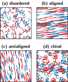
Methods Fig. 1: Snapshots of simulations of the Vicsek model. See text for a description and for the parameters used.

III Molecular dynamics simulations of the Vicsek model

We perform simple molecular dynamics simulations of a moderately large number of active agents following Eqs. (2–3) in order to visually demonstrate the disordered, flocking, antiflocking, and chiral behaviours, as shown in Extended Data Fig. 1 and SI Movie 1.

We simulate $N$ agents following Eqs. (2–3) discretized using the Euler–Maruyama scheme with a timestep $\delta t$, with a ratio $N_{A}/N_{B}$ between populations A and B, in a $L\times L$ box with periodic boundary conditions, for a duration $T_{\text{sim}}$. We choose the couplings in Eq. (2) to be $J_{mn}=J_{s(m)s(n)}H[\lVert r_{i}-r_{j}\rVert-R_{0}]$ where $s(m)$ represents the species of particle $m$ ($A$ or $B$) and $H$ is the Heaviside step function. We set $N=$512$$, $N_{A}/N_{B}=$1$$, $v_{0}=$0.5$$ $R_{0}=$2$$, $L=8$, $T_{\text{sim}}/\delta t=$8000$$ with $\delta t=$0.01$$. Figure 2a-d and SI Movie 1 show simulations exhibiting (a) disordered, (b) flocking, (c) antiflocking and (d) chiral behaviors. For these simulations, the noise is (a) $\eta=$200\text{\times}{10}^{-2}$$ and (b,c,d) $\eta=$2\text{\times}{10}^{-2}$$ and the coupling matrices $(J_{AA},J_{AB};J_{BA},J_{BB})$ are (a) $$1\text{\times}{10}^{-4}$\times(1,1;1,1)$; (b) $(1,1;1,1)$; (c) $(1,-1;-1,1)$; (d) $$0.39$\times(1,-0.25;0.25,1)$.

IV Hydrodynamic theory for non-reciprocal flocking

We have derived hydrodynamic equations for the densities $\rho_{a}(t,r)$ and polarizations $\vec{P}_{a}(t,r)$ (or equivalently the velocities $\vec{v}_{a}(t,r)$; in the main text, we denote the polarization fields by $\vec{v}_{a}(t,r)$ for simplicity) of an arbitrary number of populations from Eqs. (2–3). Our derivation, presented in the SI Sec. I, follows the methods described in Refs. Dean (1996); Bertin et al. (2006, 2009); Farrell et al. (2012); Yllanes et al. (2017); Marchetti et al. (2013); Chaté and Mahault (2019). The set of hydrodynamic equations obtained generalize the Toner-Tu equations Toner and Tu (1995, 1998) to several populations with non-reciprocal interactions, and are the basis of the analysis in the main text.

Our results for two populations also generalize the situation considered in Ref. Yllanes et al. (2017), which considers aligners A (standard Vicsek-like self-propelling particles) and dissenters B that do not align at all with anyone (neither A or B), but with which the population A aligns. With our notations, this corresponds to $j_{AA},j_{AB}>0$ but $j_{BB}=j_{BA}=0$.

Several methods of deriving continuum hydrodynamic equations from microscopics were applied to active matter, going from (i) approaches based on the Fokker–Planck (Smoluchowski) equation for the hydrodynamic variables Dean (1996); Farrell et al. (2012); Marchetti et al. (2013), to (ii) kinetic theory approaches based on the Boltzmann equation Bertin et al. (2006, 2009); Peshkov et al. (2014), or (iii) directly from the Chapman-Kolmogorov equation Ihle (2011) (in increasing order of complexity). Although coarse-graining microscopic models provides invaluable qualitative insights on the behaviour of the system, even current state-of-the-art coarse-graining procedures only provide a qualitative agreement, at best semi-quantitative, with the microscopic starting point Chaté and Mahault (2019); Mahault et al. (2019). With this in mind, we use the easiest coarse-graining method (i) along with several simplifying approximations (see SI Sec. I). This procedure has the benefit of simplicity and allows to highlight the key features of a non-reciprocal multi-component fluid. However, the correspondence between the resulting hydrodynamic equations and the microscopic model is only qualitative, in the sense that the values of the coefficients might be inaccurate.

Here, we write the hydrodynamic equations for two populations $a=A,B$. We refer to SI Sec. I for the general case of an arbitrary number of populations and its derivation from the microscopic equations.

The continuity equation reads

$$\partial_{t}\rho_{a}+v_{0}^{a}\operatorname{div}(\vec{P}_{a})=0.$$ (10)

while the equation of motion for the polarizations reads

$$\begin{split}\partial_{t}\vec{P}_{A}=\left[j_{AA}\rho_{A}-\eta-\frac{1}{2\eta}\lVert j_{AA}\vec{P}_{A}+j_{AB}\vec{P}_{B}\rVert^{2}\right]\vec{P}_{A}+j_{AB}\rho_{A}\vec{P}_{B}\\ -\frac{v_{0}^{A}}{2}\nabla\rho_{A}+D_{A}\nabla^{2}\vec{P}_{A}\\ +\lambda_{AA}\left[5/2\nabla(\vec{P}_{A}\cdot\vec{P}_{A})-3(\vec{P}_{A}\cdot\nabla)\vec{P}_{A}-5\vec{P}_{A}\operatorname{div}(\vec{P}_{A})\right]\\ +\lambda_{AB}\left[(\vec{P}_{B}\cdot\nabla)\vec{P}_{A}-2(\vec{P}_{A}\cdot\nabla)\vec{P}_{B}-2\vec{P}_{B}\operatorname{div}(\vec{P}_{A})+(\vec{P}_{B}^{*}\cdot\nabla)\vec{P}_{A}^{*}+2(\vec{P}_{A}^{*}\cdot\nabla)\vec{P}_{B}^{*}+2\vec{P}_{B}^{*}\operatorname{div}(\vec{P}_{A}^{*})\right]\end{split}$$ (11)

Here, $j_{ab}=\frac{R_{0}^{2}}{2}\,J_{ab}$ where $R_{0}$ is a characteristic length scale. The equation for $B$ is obtained by exchanging the indices. In this equation, the notation $\vec{U}^{*}$ denotes the 2D vector $\vec{U}=(U_{x},U_{y})$ rotated by 90 in the clockwise direction, namely $\vec{U}^{*}=(U_{y},-U_{x})$. The polarizations denoted by $\vec{P}_{A}$ and $\vec{P}_{B}$ here and in the SI are called $\vec{v}_{A}$ and $\vec{v}_{B}$ in the main text. The hydrodynamic parameters in Eq. (11) are related to the microscopic parameters, see SI Sec. I. When considering uniform fields, Eq. (11) reduces to

$$\partial_{t}\begin{pmatrix}\vec{P}_{A}\\ \vec{P}_{B}\end{pmatrix}=\begin{pmatrix}\alpha_{A}[\vec{P}_{A},\vec{P}_{B}]&\ j_{AB}\rho_{A}\\ j_{BA}\rho_{B}&\alpha_{B}[\vec{P}_{A},\vec{P}_{B}]\end{pmatrix}\begin{pmatrix}\vec{P}_{A}\\ \vec{P}_{B}\end{pmatrix}$$ (12)

where

$$\alpha_{A}=j_{AA}\rho_{A}-\eta-\frac{1}{2\eta}\lVert j_{AA}\vec{P}_{A}+j_{AB}\vec{P}_{B}\rVert^{2}.$$ (13)

Again, the equation for $B$ is obtained by exchanging the indices. This equation is used to construct the phase diagrams of Fig. 2, see SI Sec. II. We find (a) a disordered regime where the order parameter vanishes, (b) a flocking regime where the order parameters are parallel, (c) an antiflocking regime where the order parameters are antiparellel (sharing some similarities with Refs. Oza and Dunkel (2016); Suzuki et al. (2015); Nishiguchi et al. (2017)), (d) a periodic chiral regime where the order parameter have circular trajectories (sharing similarities with chiral active matter Tsai et al. (2005); Liebchen and Levis (2017); Banerjee et al. (2017); Souslov et al. (2019); Soni et al. (2019); Han et al. (2020)), (e) a periodic swap regime where the order parameter oscillate along a fixed direction, (f) a quasiperiodic chiral+swap regime in which the order parameter oscillates along a rotating direction. Equation (11) is then linearized above the uniform solution of Eq. (12) to obtain the stability diagram of Fig. 3 (see SI Sec. III for details on the computations).

V Simulations of the continuum equations in exceptional point induced pattern formation

To explore the pattern formation beyond linear stability, we directly solve the hydrodynamic equation (11) under periodic boundary conditions using the open-source pseudospectral solver Dedalus Burns et al. (2020). For simplicity, we focus on Eq. (11) only and assume that the fluctuations of the densities $\rho_{a}$ are high-frequency modes that can be ignored and integrated out and set $\rho_{a}\approx\text{const.}$, but we do not enforce the incompressibility constraint $\operatorname{div}(\vec{v}_{a})=0$ that would arise from Eq. (10) in a system where mass is conserved. In the SI Sec. XI, we show that pattern formation also occurs when the incompressibility constraint $\operatorname{div}(\vec{v}_{a})=0$ is enforced, both through a linear stability analysis and simulations of the non-linear hydrodynamic equations. The simulations in Fig. 3(c-g) are performed on a box of size $2L\times 2L$ with $L=$0.32$$. Each dimension is discretized with $N={2^{6}}$ modes. A random initial condition (in space, with the value at each point drawn independently from a uniform distribution on $[-1,1]$) is evolved in time with the time-stepper SBDF2 (second-order semi-implicit backwards differentiation formula) implemented in Dedalus Burns et al. (2020); Wang and Ruuth (2008) with a constant time step $\delta t=$0.01$$ for a total time $T_{\text{sim}}\approx$2000$$.

VI Phase transitions and bifurcations

In this section, we first review standard relations between phase transitions and bifurcations of dynamical systems. We then discuss our results from the point of view of bifurcation theory Arnold (1988); Kuznetsov (2004); Golubitsky and Schaeffer (1985); Golubitsky et al. (1988); Golubitsky and Stewart (2002); Chossat and Lauterbach (2000). The exceptional transitions analysed in the main text are closely related to Bogdanov-Takens bifurcations Bogdanov (1981a, b); Takens (1974); Kuznetsov (2004). At first sight, a striking difference is present: the Bogdanov-Takens (BT) bifurcation has codimension two (i.e., two parameters have to be adjusted to get to the bifurcation), while the exceptional transitions in our work have codimension one (i.e., a single parameter has to be adjusted; hence, we observe transition lines in a 2D phase diagram). We argue that this apparent tension is solved because the Goldstone theorem effectively reduces the codimension of BT bifurcations from phases with a spontaneously broken continuous symmetry.

VI.1 Phase transitions and dynamical systems

Equilibrium phase transitions are usually described in terms of a free energy. The minimum of the free energy corresponds to the current phase, and a phase transition occurs when it ceases to be a global minimum, or a minimum at all. Although this landscape picture is static, it relies on an underlying dynamics that shepherds the system into the global minimum in a way or another Landau and Khalatnikov (1954); Hohenberg and Halperin (1977); Cross and Hohenberg (1993). For instance, it arises naturally when one considers a Ginzburg-Landau-Wilson Hamiltonian obtained from renormalizing a microscopic Hamiltonian Wilson (1974); Hohenberg and Krekhov (2015) instead of a phenomenological Ginzburg-Landau free energy.

The most simple dynamics is relaxational. In this case, the dynamical system that describes the time evolution of the order parameter $\phi$ near its equilibrium value reads Landau and Khalatnikov (1954); Hove (1954); Hohenberg and Halperin (1977); Cross and Hohenberg (1993); Hohenberg and Krekhov (2015)

$$\frac{\partial\phi}{\partial t}=-\frac{\delta F}{\delta\phi}$$ (14)

for a system described by the Ginzburg-Landau free energy $F[\phi]$. Phase transitions can be seen as bifurcations of this dynamical system Laguës and Lesne (2003); Muñoz (2018); Sornette (2000).

Let us immediately note that this point of view naturally encompasses out-of-equilibrium systems, for they have an equivalent of equation (14) even when they are not described by a free energy (and more generally, when they do not possess a Lyapunov function). For instance, this occurs in non-equilibrium pattern formation Cross and Hohenberg (1993); Saarloos (1994); Aranson and Kramer (2002); Hohenberg and Krekhov (2015) (we refer to (Cross and Hohenberg, 1993, III.A.5) for a discussion on the difference between bifurcations and thermodynamic phase transitions; here, we will use liberally the term “phase transition” to describe both situations).

As an example, consider the paramagnet/ferromagnet transition of the Ising model, for which the Ginzburg-Landau free energy density reads $f(\phi)=(a/2)\phi^{2}+(b/4)\phi^{4}+(c/2)(\nabla\phi)^{2}$. This free energy describes any real-valued scalar order parameter $\phi$ with inversion symmetry $\phi\to-\phi$, which also include other systems such as incompressible symmetric binary mixtures Barrat and Hansen (2003). Applying equation (14) gives

$$\partial_{t}\phi=-a\phi-b\phi^{3}+c\Delta\phi.$$ (15)

For uniform order parameters, the Laplacian $\Delta\phi$ vanishes and we recognize the normal form of a supercritical pitchfork bifurcation, up to rescaling of the parameters. It is instructive to analyze the stability of the equilibrium solutions $\phi_{0}=0$ and $\phi_{\pm}\equiv\sqrt{-a/b}$ of this dynamical system by linearizing (14) around equilibria $\phi_{\text{ss}}$ and computing a Fourier transform to momentum space. Writing $\phi=\phi_{\text{ss}}+\delta\phi$, we find

$$\frac{\partial\delta\phi}{\partial t}=\left[-a-3b\phi_{\text{ss}}^{2}+c\nabla^{2}\right]\delta\phi+\mathcal{O}(\delta\phi^{2}).$$ (16)

In momentum space (where $k$ is the momentum),

$$\frac{\partial\delta\phi}{\partial t}=-\left[a+3b\phi_{\text{ss}}^{2}+ck^{2}\right]\delta\phi.$$ (17)

Hence, the growth rates of the Fourier modes $\delta\phi(k)$ of the perturbation are $\sigma_{0}=-a-ck^{2}$ for the trivial equilibrium $\phi=0$, and $\sigma_{\pm}=2a-ck^{2}$ for the two non-trivial equilibria (when they exist).

At the transition, the growth rate of the long-wavelength perturbations (i.e., at $k=0$) vanishes (in the ordered phase, it is negative, meaning that the perturbations are damped). In the language of high-energy physics, a massive (i.e, gapped) mode becomes massless (i.e., gapless). This is a standard mechanism for phase transitions: global fluctuations (i.e., with arbitrarily large wavelength) becomes less and less damped in time, until the transition where they are not damped anymore.

VI.2 Relations with bifurcation theory

In the main text, we show that the phase transition between the aligned phase (or antialigned) and the chiral phase are marked by the presence of an exceptional point (EP) in the linearized dynamical system (hence, we refer to these as exceptional transitions). From the point of view of bifurcation theory, this is a Bogdanov-Takens (BT) bifurcation Bogdanov (1981a, b); Takens (1974), precisely characterized by the occurrence of an exceptional point (equivalently, a Jordan block of size two), see Ref. Kuznetsov (2004). A direct computation of the linearized operator at a typical point in the exceptional transition line (in red in Fig. 2b-c) confirms that its (real) eigenvalues satisfy $\lambda_{1}=\lambda_{2}=0<\lambda_{3}<\lambda_{4}$ (in this section, we order eigenvalues by decreasing real part, so $\lambda_{1}$ is the most unstable), see also SI Sec. II for an analytical proof on the occurrence of EPs. However, the BT bifurcation has codimension two (i.e., two parameters have to be adjusted to get to the bifurcation), so BT bifurcations are typically points in a two-dimensional parameter space. In contrast, the exceptional transitions in our work have codimension one (i.e., a single parameter has to be adjusted), and we observe transition lines in the two-dimensional phase diagram Fig. 2b-c. We note that the phase diagram in Fig. 2b-c is not fine-tuned (besides the $O(2)$ symmetry of the dynamical system): the existence of transition lines persists even if we perturb the dynamical system, see below.

To solve this puzzle, let us analyze the bifurcation conditions that characterize the BT bifurcation, and how they usually lead to a codimension two. The codimension of subspaces with equal eigenvalues is a nontrivial problem, see Refs. von Neumann and Wigner (1929); Arnol’d (1972); Arnold (1995); Seyranian et al. (2005). The BT transition occurs at an equilibrium point where the Jacobian has a vanishing eigenvalue of algebraic multiplicity two $\lambda_{1}=\lambda_{2}=0$. Such a degeneracy can occur in two ways: at an exceptional point (EP) where the eigenvectors become collinear, or at a diabolic point (DP, also known as Dirac point) where the eigenvectors stay linearly independent. DPs have a considerably higher codimension that EPs (so they can essentially be ignored), see Extended Data Fig. 2; they do not correspond to the BT bifurcation (see e.g. Refs. Julien (1994); Renardy et al. (1999) for the corresponding codimension 4 bifurcation). For real matrices, the codimension of EPs is one; combined with the condition that the degenerate eigenvalues must vanish, this gives a codimension two to the BT bifurcation.

The reason why the codimension is different here lies in symmetry. A direct inspection shows that the dynamical system Eq. (11) is invariant under the group $O(2)$ of orthogonal transformations (acting diagonally, i.e. on all populations at the same time). We first note that the phase transitions in Fig. 2b-c are not Takens-Bogdanov bifurcations with $O(2)$ symmetry in the sense of Ref. Guckenheimer (1986); Dangelmayr and Knobloch (1987), because the stable eigenvalues $0<\lambda_{3}\neq\lambda_{4}$ are generally different. This is because we are considering the departure from a (time-independent) ordered phase that spontaneously breaks the $O(2)$ symmetry (such as the aligned phase), not from a fully symmetric steady-state (such as the disordered phase). (This could be analyzed as a secondary bifurcation through mode interactions Golubitsky and Schaeffer (1985); Golubitsky et al. (1988); Golubitsky and Stewart (2002) or with the formalism of Refs. Krupa (1990); Field (1980).) A crucial consequence of the spontaneous breaking of a continuous symmetry is the appearance of modes with vanishing frequency and growth rate at large wavelength called Nambu-Goldstone modes. This property is known as the Goldstone theorem, see Refs. Nambu (1960); Goldstone (1961); Goldstone et al. (1962); Hidaka (2013); Watanabe (2020); Watanabe and Murayama (2012); Nielsen and Chadha (1976), and we note that it applies to dynamical systems (not only Hamiltonian systems), see Refs. Leroy (1992); Minami and Hidaka (2018); Hongo et al. (2019); Watanabe (2020). Because of the Goldstone theorem, one eigenvalue $\lambda_{1}=0$ always vanishes in the static phases with a spontaneously broken continuous symmetry (such as the aligned and antialigned phases). In this situation, the codimension of the BT transition is simply the codimension of EPs, which is one. (More precisely, it is the codimension of EPs in the space of matrices with at least one zero eigenvalue.) To summarize, the existence of a Goldstone mode associated with a spontaneously broken continuous symmetry effectively reduces the codimension of BT bifurcations by one, leading to lines of BT bifurcations from the phase with broken symmetry in a two-dimensional phase diagram,

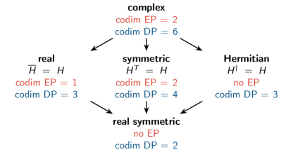
Methods Fig. 2: Codimensions of eigenvalue degeneracies. This graph gives the codimension (codim) of two-fold degeneracies of eigenvalues in different matrix spaces, see Ref. Seyranian et al. (2005). These degeneracies can be exceptional points (EP) or diabolic points (DP, also known as Dirac points). An identical graph can be drawn by replacing “real symmetric” with “purely imaginary symmetric”, “Hermitian” with “anti-Hermitian” and “real” with “imaginary”.

If the existence of Bogdanov-Takens lines is indeed due to the $O(2)$ symmetry through the Goldstone theorem, BT lines should persist under any (small) perturbation that preserves the $O(2)$ symmetry of the dynamical system. A full analysis using the methods of equivariant bifurcation theory is outside of the scope of this work; instead, we now provide numerical evidences that support our hypothesis. To do so, we consider the dynamical system

$$\partial_{t}\vec{P}_{a}=\alpha_{ab}\vec{P}_{b}+\beta_{abcd}\braket{\vec{P}_{b},\vec{P}_{c}}\vec{P}_{d}$$ (18)

which includes all $O(2)$-symmetric terms up to order three in $\vec{P}_{a}$ (see e.g. Ref Dangelmayr and Knobloch (1987); we can choose $\beta_{abcd}=\beta_{acbd}$ by symmetry of the Euclidean scalar product, so there are a total of $n^{2}+n\times n(n+1)/2\times n$ parameters in this dynamical system for $n$ populations [$16$ for $n=$2$$], two of which might be removed by rescalings). We start from values of the parameters corresponding to the dynamical system Eq. (11), and add (small) perturbations, see Extended Data Fig. 3. The figure shows that lines of exceptional points marking (anti)aligned/chiral transitions persist under a (small enough) generic $O(2)$-preserving perturbation. This strongly suggests that this phenomenon is not the result of a fine-tuning of some parameters not accounted for in our particular model.

Our argument assumes that time-independent steady-states form a submanifold of codimension zero. This is not always the case. For instance, this is not true when the symmetry group is reduced to $SO(2)$ (instead of $O(2)$). Correspondingly, the codimension of the BT bifurcation becomes higher (we find codimension 2 points in the systems analyzed in the main text, but not all possible terms are considered). Physically, this is because there are parameters (e.g., external torques) that drive the Goldstone mode in a given direction (we interpret this as an explicit PT-symmetry breaking).

In the main text, we have described the appearance of time-dependent phases as a dynamical restoration of (part of) the spontaneously broken symmetries. The main idea is that a continuous group of symmetries $G$ that is spontaneously broken to a subgroup $H\subset G$. A time-independent steady-state can be represented by a point in $G/H$ (the “manifold of degenerate ground states”), while a limit cycle corresponds to a loop $\mathcal{C}$ in $G/H$ (we assume that the motion can be made harmonic, e.g. by a nonlinear change of variables and a reparameterization of time; in the instances of the chiral phase analyzed in the main text, the motion is already harmonic and hence the loop is traveled at constant velocity). With this picture in mind, the class I defined in the main text corresponds to situations in which some operation in $H$ exchanges clockwise and counterclockwise motions on $\mathcal{C}$ (like parity does in the case of $O(2)$), while class II corresponds to situations in which there is no such operation. In class II, there is a predefined sense of rotation on the loop $\mathcal{C}$ (corresponding to an explicitly broken PT symmetry), while there is not in class I (in which the onset of a rotation either clockwise or counterclockwise along $\mathcal{C}$ would be a manifestation of a spontaneous PT symmetry breaking).

The partial restoration of spontaneously broken symmetries through the appearance of time-dependent phases also occurs for discrete groups (though not through an exceptional point). For instance, the swap phase corresponds to a $\mathbb{Z}_{2}$ symmetry. Near the transition, the order parameters approach square functions corresponding to discrete jumps between the two states related by the broken $\mathbb{Z}_{2}$ symmetry (orthogonal to the common direction of the order parameters in the (anti)aligned phase), leading to the rich harmonic content in Fig. 2g. In contrast, the continuous $SO(2)$ symmetry restored by the chiral phase corresponds to a harmonic motion (i.e., there is a fundamental frequency without higher harmonics), by which the continuous manifold of degenerate ground state is continuously traveled, with all points equivalent.

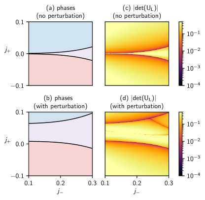
Methods Fig. 3: Effect of generic symmetry-preserving perturbations. We compare (a,c) a portion of the phase diagram from Fig. 2 to (b,d) the same portion of the phase diagram, after a generic $O(2)$-symmetric perturbation. We plot (a,b) the phase diagrams and (c,d) the absolute value of the determinant of the matrix $U_{L}$ of eigenvectors of $L(k=0)$. The vanishing of the determinant in (c,d) marks exceptional points (EPs). The phase boundaries are modified, but the topology of the diagram is not modified by small perturbations, and lines of EPs still mark the transition between (anti)aligned and chiral phases. Direct inspection of the spectrum of $L$ shows that the EPs indeed correspond to the coalescence of the two most unstable eigenvalues $\lambda_{1}$ and $\lambda_{2}$. We also note the existence of additional lines of EPs inside the chiral phase in the perturbed case. These are not the subject of the present analysis. We have used the same parameters as in figure 2 with $\eta/\eta_{\text{c}}=$0.5$$. For the perturbed case (b,d), the deviations $\Delta p$ of the parameters $p$ from the unperturbed case are $\Delta\beta_{AAAA}$ = $-0.015$, $\Delta\beta_{AABA}$ = $-0.035$, $\Delta\beta_{ABBA}$ = $-0.045$, $\Delta\beta_{BAAB}$ = $-0.025$, $\Delta\beta_{BABB}$ = $-0.045$, $\Delta\beta_{BBBB}$ = $-0.065$, $\Delta\beta_{AAAB}$ = $-0.01$, $\Delta\beta_{AABB}$ = $-0.03$, $\Delta\beta_{ABAB}$ = $-0.05$, $\Delta\beta_{ABBB}$ = $-0.07$, $\Delta\beta_{BAAA}$ = $-0.02$, $\Delta\beta_{BABA}$ = $-0.04$, $\Delta\beta_{BBAA}$ = $-0.06$, $\Delta\beta_{BBBA}$ = $-0.08$, $\Delta{j}_{AA}$ = $0.05$, $\Delta{j}_{BB}$ = $0.01$, $\Delta\rho_{A}$ = $-0.05$, $\Delta\rho_{B}$ = $0.04$.

VII Non-reciprocal Kuramoto model

In this section, we provide details on the analysis of the non-reciprocal Kuramoto model Kuramoto (1984); Acebrón et al. (2005); Sakaguchi and Kuramoto (1986); Daido (1992, 1987); Omata et al. (1988); Hong and Strogatz (2011a, b); Martens et al. (2009); Bonilla et al. (1998); Uchida and Golestanian (2010); Hong and Strogatz (2012); Ott and Antonsen (2008); Abrams et al. (2008); Pikovsky and Rosenblum (2008); Martens et al. (2016); Choe et al. (2016); Gallego et al. (2017). Depending on whether the system is in class I or in class II (PT-symmetric or not), we find codimension 2 or codimension 1 exceptional points around which the phase diagram is organized. In class I, the exceptional line (in a 2D phase diagram) separate static (aligned or antialigned) phases from a chiral phase where parity (equivalent here to PT-symmetry) is spontaneously broken. In class II, an exceptional point structures the phase diagram: the stable steady-states are organized on a truncated version of the Riemann surface of the square root. This leads to discontinuous transitions marked by hysteresis between regions where two stable states coexist and regions where only one state exists, in a similar manner to driven-dissipative quantum fluids Hanai et al. (2019); Hanai and Littlewood (2020). We first present analytic self-consistency arguments where the existence of static or harmonic steady-state is assumed. We then resort to numerical simulations of a reduced dynamical system to confirm our analytic predictions and explore the full phase diagram, including non-harmonic time-dependent phases.

VII.1 General considerations

We start from Eq. (2) of the main text. Following the standard Kuramoto model, we consider globally coupled (all-to-all) oscillators, and neglected the noise $\eta(t)\equiv 0$. The oscillators are separated into two communities $A$ and $B$, and the dynamics of the oscillators separated into two populations reads

$$\partial_{t}\theta_{m}^{a}=\omega_{m}^{a}+\sum_{b}\sum_{n=1}^{N_{b}}J_{ab}\sin(\theta_{n}^{b}-\theta_{m}^{a})$$ (19)

where $a,b=A,B$ represent the two species (or communities), and where we neglected the noise for simplicity. Hence, the coupling constants $J_{mn}$ can be $J_{AA}$, $J_{AB}$, $J_{BA}$, $J_{BB}$ depending on which populations $m$ and $n$ belong to. The distribution of the natural frequencies $\omega^{a}_{m}$ in different groups may be different in general. The conventional Kuramoto model Kuramoto (1984); Acebrón et al. (2005) is recovered by setting the coupling strength to be identical, i.e. $J_{AA}=J_{AB}=J_{BA}=J_{BB}$.

Note that the similarity between Fig. 4 and the Fig. 2 of the main text can already be anticipated from the equations of motion. The Kuramoto model with the Vicsek model are very similar besides the obvious differences summarized in Table 1, when all the oscillators are identical (i.e., they have the same natural frequencies $\omega_{m}^{A}=\omega_{m}^{B}\equiv\omega_{0}$), as the common frequency $\omega_{0}$ can be absorbed by a transformation of the degrees of freedom (where the oscillators are observed in a rotating frame). As a result, we can expect similar phases as those found in Fig. 2 (such as the flocking and chiral phases) to arise. Indeed, from numerical simulation the dynamics using the methods introduced in the next section, we indeed find a surprisingly similar phase diagram to the flocking model (Fig. 4). In terms of synchronization, the disordered phase corresponds to a desynchronized phase, while the flocking, antiflocking, and chiral phases all correspond to synchronized oscillators, respectively in phase, completely out of phase, and with an arbitrary phase delay. They are respectively named incoherent state, coherent state, $\pi$-state, and traveling wave state in Refs. Hong and Strogatz (2011a); Choe et al. (2016), see also Table 1.

VII.2 Self-consistency equation for the steady-states

Following Kuramoto Kuramoto (1984), we introduce an order parameter that characterizes synchronization for each species

$$z_{a}(t)\equiv r_{a}(t)\text{e}^{\text{i}\phi_{a}(t)}=\frac{1}{N_{a}}\sum_{m=1}^{N_{a}}\text{e}^{\text{i}\theta_{m}^{a}(t)}$$ (20)

which becomes finite when the oscillators synchronize. Here, $r_{a}\geq 0$ and $\phi_{a}$ respectively characterize the phase coherence and the average phase of the component $a$.

Introducing $j_{ab}=J_{ab}N_{b}$ and

$$R_{a}\text{e}^{\text{i}\alpha_{a}}=\sum_{b}j_{ab}z_{b}$$ (21)

allows to express Eq. (19) as

$$\partial_{t}\theta_{m}^{a}=\omega_{m}^{a}+R_{a}\sin(\alpha_{a}-\theta_{m}^{a}).$$ (22)

In order to obtain a continuum equation for a large number of oscillators $N_{a}\to\infty$, we introduce the distribution of natural frequencies $g_{a}(\omega)=\frac{1}{N_{a}}\sum_{m=1}^{N_{a}}\delta(\omega-\omega_{m}^{a})$ and the density of angles $\rho_{a}(\theta;\omega,t)=\delta(\theta-\theta_{a}(\omega,t))$ where $\theta_{a}(\omega,t)$ is a solution of Eq. (22) in which $\omega_{m}^{a}$ is replaced by $\omega$ and $\theta^{a}_{m}$ by $\theta_{a}(\omega)$, with an initial condition specified by $\rho_{a}(\theta;\omega,t=0)$. The order parameter then becomes

$$z_{a}(t)=\int_{-\infty}^{\infty}d\omega\int_{-\pi}^{\pi}\text{d}\theta\text{e}^{\text{i}\theta}g_{a}(\omega)\rho_{a}(\theta;\omega,t)$$ (23)

This equation provides a self-consistency condition for the order parameter.

We focus on steady-states of the form

$$z_{a}(t)=z_{a}\text{e}^{\text{i}\Omega t}\quad\text{with}\quad z_{a}=r_{a}\text{e}^{\phi_{a}^{0}}.$$ (24)

Those must satisfy the self-consistency equation Acebrón et al. (2005)

$$z_{a}=R_{a}e^{i\alpha_{a}}F_{a}[z_{A},z_{B}],$$ (25)

where we have introduced the functions

$$\begin{split}&F_{a}[z_{A},z_{B}]=\int_{-\pi/2}^{\pi/2}\text{d}\theta\cos\theta\,\text{e}^{\text{i}\theta}g_{a}(R_{a}\sin\theta+\Omega)\\ &+\int_{-\pi}^{\pi}\text{d}\theta\int_{|x|>1}\text{d}x\,\text{e}^{\text{i}\theta}g_{a}(R_{a}x+\Omega)\frac{\sqrt{x^{2}-1}}{|x-\sin\theta|}.\end{split}$$ (26)

The first (second) term in Eq. (LABEL:Fa) is the contribution from the synchronized (unsynchronized) oscillators. Using Eq. (21), this condition can be written in the form,

$$\hat{M}[z_{A},z_{B},\Omega]\begin{pmatrix}z_{A}\\ z_{B}\end{pmatrix}=0,$$ (27)

with

$$\hat{M}[z_{A},z_{B},\Omega]=\begin{pmatrix}F_{A}^{-1}-j_{AA}&-j_{AB}\\ -j_{BA}&F_{B}^{-1}-j_{BB}\end{pmatrix}.$$ (28)

The structure of Eq. (27) is similar to Eq. (12) (obtained for non-reciprocal flocking), in the sense that the steady state condition is controlled by a nonlinear non-Hermitian $2\times 2$ matrix. This is more easily illustrated in the particular case in which $g_{A}(\omega)=g_{B}(\omega)$ is a symmetric distribution centered at $\omega_{0}$. When $|z_{a}|$ is small, we can expand $F_{a}^{-1}=\eta+\beta R_{a}^{2}+\text{i}\zeta\Omega+\mathcal{O}(\Omega^{2},\Omega R_{a},R_{a}^{2})$ where $\eta$, $\beta$, $\zeta$ are real numbers and set $\omega_{0}=0$ without loss of generality. We then find

$$\text{i}\Omega\zeta\begin{pmatrix}z_{A}\\ z_{B}\end{pmatrix}=\begin{pmatrix}\tilde{\alpha}_{A}[z_{A},z_{B}]&\!\!j_{AB}\\ j_{BA}\!\!&\tilde{\alpha}_{B}[z_{A},z_{B}]\end{pmatrix}\begin{pmatrix}z_{A}\\ z_{B}\end{pmatrix}$$ (29)

where $\tilde{\alpha}_{a}=-\eta+j_{aa}-\beta R_{a}^{2}$. This equation has a remarkable resemblance to Eq. (12) (with $\partial_{t}\to\text{i}\Omega$). This suggests that in this particular case, the transition from the phase corresponding to the flocking/antiflocking phase ($\Omega=0$) to one corresponding to the chiral phase ($\Omega\neq 0$) takes place at an exceptional point of $\hat{M}$.

However, an important difference arises in the general case where $g_{A}(\omega)\neq g_{B}(\omega)$: as the (generalized) PT symmetry is explicitly broken by the presence of natural frequencies, the matrix $\hat{M}$ in Eq. (27) is complex-valued, in contrast with the matrix in Eq. (12) that is real-valued. As a consequence, exceptional points should occur at points in a two-dimensional parameter space, rather than along lines such as in Figs. 2b-c (i.e., their codimension is two; see also the discussion in the section VI Phase transitions and bifurcations). This is consistent with the occurrence of Bogdanov-Takens points in generalized Kuramoto models Choe et al. (2016); Gallego et al. (2017); Pazó and Montbrió (2009); Pietras et al. (2018); Martens et al. (2016); Bonilla et al. (1998), in which hysteresis can be present Pazó and Montbrió (2009); Pietras et al. (2018). This situation is similar to the case of quantum fluids analyzed in Refs. Hanai et al. (2019); Hanai and Littlewood (2020), where a first-order-like phase transition associated with a jump in physical quantities may arise with an exceptional point marking the endpoint of the phase boundary. To further investigate it, we now analyze the mean-field dynamics of the non-reciprocal Kuramoto model.

VII.3 Mean-field dynamics in the Ott-Antonsen manifold

The dynamics of the generalized Kuramoto model in Eq. (2) can exactly be captured by a small number of coupled differential equations in the limit of a large number of oscillators, see Refs. Ott and Antonsen (2008, 2009); Watanabe and Strogatz (1993, 1994); Marvel et al. (2009); Pikovsky and Rosenblum (2011, 2008); Hong and Strogatz (2011a, b, 2012); Tyulkina et al. (2018); Montbrió et al. (2015) and the review Ref. Bick et al. (2020). In SI Sec. VI, we have demonstrated that this mean-field dynamics is quantitatively consistent with direct simulation of microscopic model Eq. (2).

Through this mean-field reduction, the evolution of the complex order parameter $z_{a}(t)$ for each community $a$ is described by Ott and Antonsen (2008)

$$\partial_{t}z_{a}=(\text{i}\omega_{a}-\Delta_{a})z_{a}+\frac{1}{2}\sum_{b}j_{ab}\left[z_{b}-z_{a}^{2}\,\overline{z_{b}}\right].$$ (30)

where $\overline{z_{b}}$ is the complex conjugate of $z_{b}$. We assumed that the natural frequencies of the oscillators in the community $a$ follow a Lorentzian distribution $g_{a}(\omega)=\pi^{-1}\,[(\omega-\omega_{a})^{2}+\Delta_{a}^{2}]^{-1}$. The term $\text{i}\omega_{a}z_{a}$ in Eq. (30) explicitly breaks the mirror symmetry $z_{a}\to\overline{z_{a}}$ (and hence, breaks parity), but is invariant under rotations $z_{a}\to\text{e}^{\text{i}\theta}z_{a}$.

When $\omega_{a}=0$ for all the communities, the system has a full $O(2)$ symmetry, and one observes phases with spontaneously broken parity. In this paragraph, we focus on this situation. To mirror the analysis in the main text, we define $j_{\pm}=[j_{AB}\pm j_{BA}]/2$ and determine a numerical phase diagram of the system in the $(j_{-},j_{+})$ plane, see Extended Data Fig. 4. This phase diagram shares several qualitative features with the flocking phase diagram in Fig. 2 in the main text. In particular, we find that the phase boundaries between the (anti)synchronized state (labeled coherent and $\pi$-state in Extended Data Fig. 4) and the chiral state (labeled traveling wave in Extended Data Fig. 4) are marked by exceptional points in the Jacobian $L$ of the dynamical system Eq. (30). Writing the right-hand side of Eq. (30) as $f_{a}(z_{b})$, the $4\times 4$ Jacobian matrix $L$ has blocks

$$L_{ab}=\begin{pmatrix}{\partial f_{b}}/{\partial z_{a}}&{\partial f_{b}}/{\partial\overline{z_{a}}}\\ {\partial\overline{f_{b}}}/{\partial z_{a}}&{\partial\overline{f_{b}}}/{\partial\overline{z_{a}}}\\ \end{pmatrix}$$ (31)

for $a,b=A,B$, where the derivatives are evaluated at the steady-state. A direct numerical evaluation of this matrix shows that the two most unstable eigenvalues indeed coalesce (i.e., form an exceptional point) at the transition, see Extended Data Fig. 5 for an example.

To analyze the situation with explicitly broken PT symmetry (class II), we introduce a finite detuning $\Delta\omega=\omega_{A}-\omega_{B}$ between the natural frequencies of the two communities (we keep $\omega_{A}+\omega_{B}=0$ for simplicity). The numerical simulation of Eq.(30) show that there are regions of the phase diagram in which two states (clockwise and counterclockwise) coexist, as well as regions in which a single state is present. This can be understood as the result between the spontaneous PT-symmetry breaking at $\Delta\omega=0$ (in which the two states are equivalent, and mapped to each other by PT symmetry) and the detuning that explicitly breaks PT symmetry. At the boundary between these regions, the properties of the steady-states (such as their frequency $\Omega_{\text{ss}}\equiv\Omega$) change in a discontinuous way (like in a first-order phase transition). This is illustrated in Extended Data Fig. 6. In Extended Data Fig. 6a, we show the manifold of stable steady-states obtained from numerical simulations, which is a truncated version of the Riemann surface of the square root characteristic of exceptional points. There is coexistence between two states (blue and red dots) in the red region in parameter space. In Extended Data Fig. 6b, we show hysteresis curved corresponding to slices of the manifold represented Extended Data Fig. 6a.

This behavior shares some features with the dynamical encircling of an exceptional point in a linear system Doppler et al. (2016); Dembowski et al. (2004); Milburn et al. (2015); Mailybaev et al. (2005). However, a crucial difference is that here, we are dealing with the steady-state (i.e., many-body phase) of the system, which is possible only because of the non-linearity (similar situations occur in Refs. Hanai et al. (2019); Galda and Vinokur (2016, 2019); Kepesidis et al. (2016); Graefe et al. (2010); Cartarius et al. (2008); Gutöhrlein et al. (2013); Strack and Vitelli (2013)). In addition, the breakdown of the adiabatic theorem plays a crucial role in the situations analyzed in Refs. Doppler et al. (2016); Dembowski et al. (2004); Milburn et al. (2015); Mailybaev et al. (2005), but it is not the case in the first-order-like transitions and hysteretic behavior described here. In particular, the hysteresis observed in Extended Data Fig. 6 does not depend on the speed at which the parameters are changed ($\Delta\omega$ in Extended Data Fig. 6b), provided that the change is slow enough (so that the system is always in a steady-state). The hysteresis curve is then independent of the arbitrarily small rate of change. This is in sharp contrast with the situations analyzed in Refs. Doppler et al. (2016); Dembowski et al. (2004); Milburn et al. (2015); Mailybaev et al. (2005), ruled by a linear dynamical system, in which the most unstable state (i.e., the one with the largest positive growth rate) always eventually dominates given enough time: in this situation, there is no hysteresis in the limit of an arbitrarily small rate of change.

flocking	synchronization
active agents	oscillators
typically short-range	typically all-to-all
external torque	natural frequency
self-propulsion	n/a
disordered	incoherent
flocking	coherent
antiflocking	$\pi$-state
chiral	traveling wave state (TW)
swap	periodic synchronization (PS)
swap+chiral	PS+TW

Methods Table 1: A flocking-synchronization Rosetta stone. We compare the ingredients in the generalized Vicsek (flocking) and Kuramoto (synchronization) models, as well as some of their states. For synchronization, we mostly followed the nomenclature of Refs. Acebrón et al. (2005); Hong and Strogatz (2011a, b, 2012); Hong (2014); Kemeth et al. (2016); Choe et al. (2016). The literature is not entirely consistent in the choice of names and definitions of the states; our definitions are summarized in Table 2.

state	$r_{a}$	$\phi_{B}-\phi_{A}$
incoherent	$0$	n/a
coherent	constant $\neq 0$	$0$
$\pi$-state	constant $\neq 0$	$\pi$
traveling wave state	constant $\neq 0$	constant $\neq 0,\pi$
periodic synchronization	time-dependent	constant
PS+TW	time-dependent	time-dependent

Methods Table 2: Definition of the states. The complex order parameters $z_{a}=r_{a}\text{e}^{\text{i}\phi}$ are decomposed in amplitude $r_{a}=|z_{a}|$ and phase $\text{e}^{\text{i}\phi_{a}}=z_{a}/|z_{a}|$. The label “PS+TW” corresponds to “periodic synchronization + traveling wave”. Here, we make the following choices: (i) the system is observed in the lab frame (not in the rotating frame); (ii) we do not distinguish fully coherent states ($r=1$) from partially coherent ones ($0\neq r<1$), both are called “coherent”.

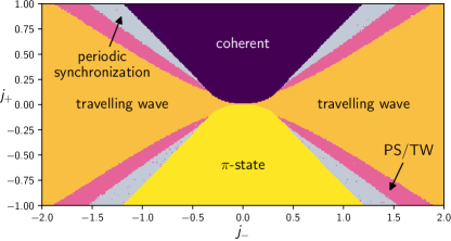
Methods Fig. 4: Phase diagram of the PT-symmetric non-reciprocal Kuramoto model. The states are defined in Table 2. We have set $j_{AA}=j_{BB}=$1$$, $\Delta_{A}=\Delta_{B}=$0.25$$ and $\omega_{A}=\omega_{B}=$0$$.

Methods Fig. 5: Exceptional point in the spectrum of the Jacobian in the Kuramoto model. The two most unstable eigenvalues $\lambda_{i}=\sigma_{i}+\text{i}\omega_{i}$ of $L$ coalesce at $j_{+}\approx$0.007$$. This value coincides with the transition from traveling waves (TW) to coherent states, marked by a red dashed line. Note that this coalescence occurs at $\lambda=0$ (not at finite frequency and/or growth rate). The corresponding eigenvectors become collinear (this can be verified, for instance, by computing the determinant of the matrix of eigenvectors, that vanishes at the EP). The imaginary parts $\omega_{i}$ (not shown) are all zero. We used the same parameters as in Extended Data Fig. 4 with $j_{-}=$0.1$$. A similar behavior is observed for neighboring values of $j_{-}$.

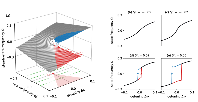
Methods Fig. 6: Hysteresis in the chiral Kuramoto model. When chirality is explicitly broken, exceptional points have codimension two, i.e. they are typically points in a two-dimensional parameter space. We plot the frequency $\Omega$ of the steady-state of the Kuramoto model with explicitly broken PT symmetry as a function of the difference $\Delta\omega=\omega_{A}-\omega_{B}$ between the two communities (also called detuning) and the deviation $\delta j_{-}=j_{-}-j_{-}^{\text{EP}}$ of the non-reciprocal part $j_{-}$ of the coupling between the communities from its value $j_{-}^{\text{EP}}$ at the exceptional point. The system exhibits a region where two possible steady-states with different properties coexist (the two steady-states are the continuation of the clockwise and counterclockwise chiral phases present in the PT-symmetric case $\Delta\omega=0$). This region (red triangle) starts at the EP (red point) and its size increases with the amount of non-reciprocity (here $j_{-}^{\text{EP}}\simeq$0.2915$>0$). The system exhibits hysteresis in the coexistence region (red points). In (b-e), we show slices at fixed $\delta j_{-}$ (marked by blue dotted lines in (a). After the EP, there is hysteresis/first-order (discontinuous) behavior. In (d), the hysteresis curve bends outwards near the transition. This is due to the oscillation of the norm of the order parameter (that we refer to swap or periodic synchronization elsewhere) for large enough $\delta j_{-}$. This additional complication does not occur for moderate values of $\delta j_{-}$, such as in (c). The solution of the dynamical system Eq. (30) were computed along lines at fixed $\delta j_{-}$, starting at large $|\delta\omega|$ (in a region without phase coexistence) from a random initial condition. The solution (after convergence) was used as an initial value for the next point in the line with fixed $\delta j_{-}$. This procedure was carried out two times, starting from positive and negative large $|\delta\omega|$. We have set $j_{+}=$0.08$$, $j_{AA}=j_{BB}=$1$$, $\Delta_{A}=\Delta_{B}=$0.25$$, $\omega_{A}=-\omega_{B}=\Delta\omega/2$.

VIII Non-reciprocal pattern-forming instabilities

In this section, we apply our general strategy to pattern-forming instabilities within the formalism of amplitude equations Cross and Hohenberg (1993); Saarloos (1994); Aranson and Kramer (2002); Hoyle (2006); Cross and Greenside (2009); Meron (2015). These describe a variety of physical systems ranging from fluid convection and lasers to ecological and chemical reaction-diffusion systems.

To clear any misunderstanding, let us warn the reader: this section is not about the exceptional-point enforced pattern formation in Fig. 3! Instead, we consider a toy model of pattern formation with two fields that are coupled in a non-reciprocal way. Here, the pattern formation is the spontaneous symmetry breaking (the Euclidean group $E(d)$ of isometries of space is broken by the appearance of the pattern).

In addition to the formalism of amplitude equations which allows for a direct parallel with the discussion in the main text, we perform direct simulations of two coupled copies of the Swift-Hohenberg equation Swift and Hohenberg (1977), a simple model of pattern formation.

We then review a slightly more complicated situation, in which a single field is present, but two Fourier modes with non-reciprocal couplings are relevant (the non-reciprocity occurs between the harmonics), in which patterns with spontaneously broken parity also occur Malomed and Tribelsky (1984); Coullet and Fauve (1985); Brachet et al. (1987); Douady et al. (1989); Coullet et al. (1989); Coullet and Iooss (1990); Fauve et al. (1991) (see also Refs. Knobloch et al. (1995); Armbruster et al. (1988); Proctor and Jones (1988); Dangelmayr et al. (1997)). This situation has several experimental realizations in directional solidification of liquid crystals Simon et al. (1988); Flesselles et al. (1991); Melo and Oswald (1990); Oswald et al. (1987), directional solidification of lamellar eutectics Faivre et al. (1989); Faivre and Mergy (1992); Kassner and Misbah (1990); Ginibre et al. (1997), directional viscous fingering Rabaud et al. (1990); Cummins et al. (1993); Pan and de Bruyn (1994); Bellon et al. (1998), and in overflowing fountains Counillon et al. (1997); Brunet et al. (2001). We show that in this situation too, the transition is marked by an exceptional point where the Goldstone mode of the spontaneously broken translation symmetry coalesces with a damped mode.

Without any attempt at completeness, we also refer to Refs. Knobloch and Proctor (1981); Cross and Kim (1988); Cross (1986); Coullet and Spiegel (1983); Cross (1988); Brand et al. (1983, 1984); Guckenheimer (1984); Moses and Steinberg (1986); Walden et al. (1985); Coullet et al. (1985); Bensimon et al. (1989); Knobloch and Moore (1990); Schöpf and Zimmermann (1993) on binary convection and to Refs. Bressloff et al. (2001, 2002); Cho and Kim (2004); Schnabel et al. (2008); Butler et al. (2011); Curtu and Ermentrout (2004); Adini et al. (1997); Hensch and Fagiolini (2005) on the visual cortex, and to Refs. Chossat and Iooss (1994); Riecke and Paap (1992); Tennakoon et al. (1996); Mutabazi and Andereck (1995); Bot et al. (1998); Wiener and McAlister (1992); Andereck et al. (1986); Altmeyer and Hoffmann (2010); Pinter et al. (2006) on Taylor-Couette/Dean flows.

VIII.1 Coupled amplitude equations

Let us first consider the one-dimensional Ginzburg-Landau/amplitude equation

$$\partial_{t}A=\epsilon A-g|A|^{2}A+D\partial_{x}^{2}A$$ (32)

where $A$ is a complex amplitude. This equation describes, for instance, rolls in Rayleigh-Bénard convection. The physical field $u$ (such as velocity or temperature) reads $u(t,x)=A(t,x)\text{e}^{\text{i}(q_{\text{c}}x-\omega t)}+\text{c.c.}$, where $q_{\text{c}}$ is the wavenumber of the convection rolls, and $A(t,x)$ is a slowly varying envelope. The apparition of a pattern is marked by $A\neq 0$, and corresponds to the spontaneous breaking of translation symmetry. The amplitude equation (32) satisfies translation symmetry by which $A\to A\text{e}^{\text{i}\phi}$, corresponding to a translation of the pattern by a distance $\phi/q_{\text{c}}$ in the $x$ direction; as well as inversion symmetry $x\to-x$ by which $A\to\overline{A}$ (overbar is complex conjugation). The reflection does not commute with the translations, so overall we do not have the direct product of these groups, but instead the semidirect product $U(1)\rtimes Z_{2}\simeq O(2)$. This symmetry prohibits terms such as $A^{2}$ in the right-hand side of Eq. (32), and guarantees that the coefficients are real.

Let us now introduce non-reciprocity: to do so, we consider two coupled amplitudes $A_{1}$ and $A_{2}$ (describing two different coupled fields), and write the most general equation of motion compatible with the symmetry, up to third order (like in Eq. (32)). The only terms allowed are first order terms, as well as third order terms of the form $(\overline{A_{b}}A_{c}+\overline{A_{c}}A_{b})A_{d}$, in both cases with real coefficients. Hence, our amplitude equation reads

$$\partial_{t}A_{a}=\epsilon_{ab}A_{b}-g_{abcd}(\overline{A_{b}}A_{c}+\overline{A_{c}}A_{b})A_{d}+D_{ab}\partial_{x}^{2}A_{b}$$ (33)

where all the coefficients are real. In the following, we will focus on spatially uniform fields and ignore the diffusive term in Eq. (33). In hindsight, we recognize Eq. (18) upon representing the complex amplitude $A_{a}$ as a two-dimensional $P_{a}=(\text{Re}A_{a},\text{Im}A_{a})$, owing to the fact that the symmetry groups are isomorphic. We note, however, that the physical interpretation of the symmetries are quite different in both case. Having identified Eq. (33) with Eq. (18) (in the uniform case), we can immediately predict that all the phases described in the main text should appear in the current context. Our last task is then to provide a physical interpretation for each of them:

1. disordered: there is no pattern, the amplitude decays to zero

2. aligned: a pattern is present (and spontaneously breaks translational invariance, leading to a Goldstone mode often known as phase diffusion), here, the patterns for both fields are superimposed (they are in-phase)

3. antialigned: same as flocking, except that the maxima of a field now coincide with the minima of the other (they are completely out-of-phase)

4. chiral: the patterns move along $x$ (with a spontaneously chosen direction and at constant velocity), and they are partially out-of-phase (neither in-phase nor completely out-of-phase)

5. swap: the amplitude of the patterns oscillates (usually not sinusoidally)

6. chiral/swap: the patterns move along $x$ while their amplitudes fluctuate.

VIII.2 Coupled Swift-Hohenberg equations

To further support our claims and illustrate the phases described above, we consider two coupled Swift-Hohenberg equations (4) Swift and Hohenberg (1977) describing the dynamics of the real fields $u_{a}(t,x)$, with $a=1,2$ (we also define $r_{\pm}=[r_{12}\pm r_{21}]/2$). An explicit version of the amplitude equations (33) (obtained from symmetry considerations) could be derived from Eq. (4), following e.g. Ref. Saarloos (1994). Instead, we solve Eq. (4) numerically on a one-dimensional domain of size $2L$ with periodic boundary conditions using the open-source pseudospectral solver Dedalus Burns et al. (2020), starting from random initial conditions. The results confirm our predictions based on the coupled amplitude equations (33). In Extended Data Fig. 7, we show snapshots of the numerical results, in which all the phases described above appear. In this case, Eq. (4) have the full Euclidean group $E(1)$ as a symmetry group, that is broken by pattern formation. (The $O(2)$ symmetry of Eq. (33) pertains to the amplitude equation description, in which additional knowledge about the pattern is taken into account.)

VIII.3 Discussion

As we have emphasized in the introduction of this section, the pattern formation appears at different levels here compared to the main text. Here, pattern formation (as a spontaneous breaking of the Euclidean symmetry) is our starting point; we couple two pattern-forming systems in a non-reciprocal way, and observe exceptional transitions as a consequence. In particular, there is no convective term in the amplitude equation (32). Only diffusive terms are present. This is in contrast with the situation presented in Fig. 3 in the main text, where the interplay between convective terms and exceptional transitions is the origin of pattern-forming instabilities. Besides, we emphasize that we did not assume non-reciprocal cross-diffusion, in contrast with Refs. You et al. (2020); Saha et al. (2020) (another difference with these references is that we consider a non-conserved order parameter in the language of Ref. Hohenberg and Halperin (1977)). Our analysis focuses on the mean-field transitions, and our conclusions remain valid as long as the growth rates are negative at finite $k$ (this is in particular the case where $D_{ab}=D\delta_{ab}$, so the growth rates are of the form $\sigma_{i}(k)=\sigma_{i}(0)-Dk^{2}$; but this is especially not guaranteed when $D_{ab}$ is not symmetric).

We also mention that upon lifting the constraint put upon Eq. (33) by reflection symmetry, one is left with an $U(1)$-equivariant system with explicitly broken PT symmetry, as Eq. (33) becomes a complex Ginzburg-Landau equation, in which we expect the analysis of the section VII Non-reciprocal Kuramoto model to hold.

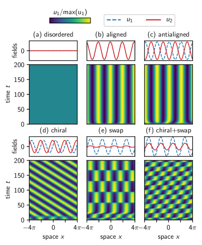
Methods Fig. 7: Non-reciprocal pattern formation We show a space-time density plot of the field $u_{1}(x,t)$ in different phases, as well as snapshots of the fields $u_{1}(x,t)$ and $u_{2}(x,t)$ at time $t=$200$$. We observe (a) a disordered phase where both field vanish, (b) an aligned phase where both patterns are static and in phase, (c) an antialigned phase where the patterns are static and completely out-of-phase, (d) a chiral phase where the patterns move at constant velocity, either to the left or to the right, and in which the fields have a finite phase difference, usually neither zero nor $\pi$, (e) a swap phase where the patterns essentially jump by a phase $\pi$ every period and (f) a mix of the chiral and swap behaviors (as in the chiral phase (d), there is a spontaneously broken symmetry between left and right movers). The fields are obtained by direct numerical simulation of the coupled Swift-Hohenberg equations on a one-dimensional domain of size $2L$ with periodic boundary conditions, starting from random initial conditions. The simulations are performed using the open-source pseudospectral solver Dedalus Burns et al. (2020). We have used $g=$0.25$$ in all cases. In (a) $r_{11}=r_{22}=$-0.5$$ and $r_{+}=r_{-}=$0.00$$. In the other cases (b-f), we have set $r_{11}=r_{22}=$0.5$$ and (b) $r_{+}=$0.50$$, $r_{-}=$0.00$$ (c) $r_{+}=$-0.50$$, $r_{-}=$0.00$$ (d) $r_{+}=$0.00$$, $r_{-}=$0.25$$ (e) $r_{+}=$0.87$$, $r_{-}=$1.00$$ (f) $r_{+}=$0.85$$, $r_{-}=$1.00$$.

VIII.4 Directional interface growth

Following Refs. Malomed and Tribelsky (1984); Douady et al. (1989); Coullet et al. (1989); Coullet and Iooss (1990); Fauve et al. (1991), we now consider a single scalar field decomposed as

$$u(t,x)=A_{1}(t,x)\text{e}^{\text{i}(q_{\text{c}}x-\omega t)}+A_{2}(t,x)\text{e}^{\text{i}(2q_{\text{c}}x-\omega t)}+\text{c.c.}$$ (34)

As in the previous case, the transition and reflection symmetry of the underlying system endows the amplitude equation with $O(2)$ symmetry. However, note that while $A_{1}$ transforms as $A_{1}\to A_{1}\text{e}^{\text{i}\theta}$ when the field $u$ is translated in space, $A_{2}$ transforms as $A_{2}\to A_{2}\text{e}^{2\text{i}\theta}$. This is a different representation of the $SO(2)$ group compared to the previous paragraph. (The $\mathbb{Z}_{2}$ part is unchanged, and still corresponds to $A_{1}\to\overline{A_{1}}$ and $A_{2}\to\overline{A_{2}}$.) Because the representation is different, the general form of the amplitude is different, and reads Malomed and Tribelsky (1984); Douady et al. (1989); Coullet et al. (1989); Coullet and Iooss (1990); Fauve et al. (1991)

$$\begin{split}\partial_{t}A_{1}&=\mu_{1}A_{1}-\overline{A_{1}}A_{2}-\alpha|A_{1}|^{2}A_{1}-\beta|A_{2}|^{2}A_{1}\\ \partial_{t}A_{2}&=\mu_{2}A_{2}+\epsilon A_{1}^{2}-\gamma|A_{1}|^{2}A_{2}-\delta|A_{2}|^{2}A_{2}\end{split}$$ (35)

The coefficients $\alpha$, $\beta$, $\gamma$ and $\delta$ are usually assumed to be positive to ensure stability, and the coefficient of $\overline{A_{1}}A_{2}$ is set to $-1$ by rescaling. The non-reciprocity is then captured by the coefficient $\epsilon$ being positive, which is necessary for the apparition of traveling patterns Douady et al. (1989). As the amplitudes $A_{1}=r_{1}\text{e}^{\text{i}\phi_{1}}$ and $A_{2}=r_{2}\text{e}^{\text{i}\phi_{2}}$ correspond to different Fourier components, the relevant phase difference between them is $\Delta\phi=2\phi_{1}-\phi_{2}$.

In Extended Data Fig. 8, we show the spectrum of the operator $L$ obtained by linearizing (35) around its steady-state (see Eq. (31) for the definition of $L$, with the replacement $z_{a}\to A_{a}$). At the transition between a static solution (representing a static pattern) and a traveling wave solution (representing a traveling pattern), we observe the coalescence of the Goldstone mode with a damped mode at an exceptional point (red circle in the figure). We also note that the presence of exceptional points away from zero in the spectrum of $L$ does not mark a phase transition (bifurcation).

Methods Fig. 8: Exceptional point in directional interface growth. The spectrum of the Jacobian $L$ corresponding to Eq. (35) exhibits an exceptional point at the transition between static patterns and traveling patterns with spontaneous parity breaking (i.e., the patterns travel with equal probability to the left or to the right). The two most unstable eigenvalues $\lambda_{i}=\sigma_{i}+\text{i}\omega_{i}$ of $L$ coalesce at $\mu_{1}\approx$0.064$$ (red circle). This value coincides with the transition from a constant solution to traveling waves (TW), marked by a red dashed line. The coalescence occurs at $\lambda=0$ (not at finite frequency and/or growth rate), and the corresponding eigenvectors become collinear. Note that another exceptional point occurs near $\mu_{1}\approx$0.014$$ (green circle), but with a strictly negative growth rate: this does not correspond to a bifurcation. We also show the dephasing $\Delta\phi=2\phi_{1}-\phi_{2}$ between the amplitudes, which undergoes a pitchfork bifurcation; the direction of motion of the pattern is set by $\Delta\phi$. We have set $\alpha=\beta=\gamma=\delta=$1$$, $\epsilon=$1$$ and $\mu_{2}=$-0.1$$.

IX Generalized PT symmetry and dynamical systems

In this section, we show how the transition from the aligned (or antialigned) phase to the chiral phase can be seen as a spontaneous PT-symmetry breaking.

Let us first review (generalized) PT-symmetry in the context of linear operators. We refer the reader to Ref. Mostafazadeh (2002a, b, c); Bender et al. (2002); Bender and Mannheim (2010); Mostafazadeh (2015) for details and proofs, and for a translation of the same concepts in the language of pseudo-Hermitian operators. Consider an antiunitary operator $X$ (i.e., there is a linear operator $M_{X}$ such that $X\psi=M_{X}\overline{\psi}$) such as $X^{2}=\text{Id}$ (where Id is the identity matrix). The operator $X$ can be seen as a generalization of the product $PT$ of parity $P$ and time-reversal $T$ (as it has the same properties), and is therefore called a (generalized) PT symmetry. This generalized PT symmetry might have nothing to do with the physical parity and time-reversal operations: only the relevant algebraic structure is kept. As $X^{2}=\text{Id}$, it is always possible to find a basis in which the antiunitary $X$ is represented by complex conjugation alone, by a reduction to Wigner normal form Weigert (2003); Wigner (1960).

Following Ref. Mostafazadeh (2015), we say that a complex square matrix $H$ is $X$-symmetric when $[H,X]=0$. The $X$-symmetry is called exact (or unbroken) when in addition, there is a complete set of eigenvectors $\psi_{n}$ of $H$ satisfying $X\psi_{n}=\psi_{n}$. Else, it is called inexact (or spontaneously broken). It can be shown that the spectrum of $H$ is real if and only if there is an antiunitary $X$ such as $H$ has an exact $X$-symmetry. In contrast with the case where PT symmetry is spontaneously broken ($H$ has an inexact $X$-symmetry), we say that PT symmetry is explicitly broken when $H$ is not $X$-symmetric.

In a non-linear dynamical system $\partial_{t}\psi=f(\psi)$, the condition of PT-symmetry reads $Xf(\psi)=f(X\psi)$, see e.g. Ref. Konotop et al. (2016).

Consider a harmonic solution of the form $\psi(t)=\text{e}^{st}\psi_{0}$ where $s=\sigma+\text{i}\Omega$ is a complex growth rate (we are mostly interested in the case where $s=\text{i}\Omega$ is purely imaginary). It satisfies $\partial_{t}\psi(t)=s\psi(t)$ (whether the system is PT-symmetric or not; this crucial property hinges on the fact that the motion is harmonic, and that (at least the relevant part of) the order parameter is written as a complex number, see Refs. Golubitsky and Stewart (1985); Marques et al. (2013); Haragus and Iooss (2011)). Further assuming that $f$ is $U(1)$-equivariant (with $f(\text{e}^{\text{i}\theta}\psi)=\text{e}^{\text{i}\theta}f(\psi)$), we find $f(\psi(t))=\text{e}^{st}f(\psi_{0})$, leading to $s\psi_{0}=f(\psi_{0})$. Using PT-symmetry, we deduce $\overline{s}X\psi_{0}=Xf(\psi_{0})=f(X\psi_{0})$. Hence, $X\psi_{0}=\psi_{0}$ implies that $s$ is real. Conversely, given a solution $\psi_{0}$ with a complex growth rate $s\not\in\mathbb{R}$ that is not purely real, we find that $X\psi_{0}$ is another solution with complex growth rate $\overline{s}$. (When $f(\psi)=H(\psi)\psi$ where $H(\text{e}^{\text{i}\theta}\psi)=H(\psi)$ is $U(1)$-invariant, the properties above can be reformulated in terms of the non-linear eigenvalue problem $s\psi_{0}=H(\psi_{0})\psi_{0}$, in which the analogy with standard PT-symmetry is more obvious. This is however not required.)

The procedure described above can be carried out for the systems in the main text, provided that we consider the complex order parameters $z_{a}=v_{a}^{x}+\text{i}v_{a}^{y}$. In this representation, a $SO(2)\simeq U(1)$ rotation corresponds to the multiplication by a phase $z_{a}\to\text{e}^{\text{i}\theta}z_{a}$ while mirror symmetry corresponds to complex conjugation $z_{a}\to\overline{z_{a}}$. Hence, systems in both class I and II correspond to $U(1)$-equivariant dynamical systems. Besides, systems in class I are PT-symmetric (with $X$ being complex conjugation), while systems in class II are not PT-symmetric (the parameters in $\alpha^{*}$ and $\beta^{*}$ explicitly break PT-symmetry). Note that here, the physical parity (mirror symmetry) corresponds to the PT-symmetry.

The same strategy should allow for multiple frequencies, provided that they correspond to independent components of the order parameter, by generalizing the equation $f(\psi_{0})=s\psi_{0}$ to $f(\psi_{0})=\text{diag}(s_{1},s_{2},\dots)\psi_{0}$. As an example, consider the case of directional interface growth presented in the section VIII Non-reciprocal pattern-forming instabilities. The two complex amplitudes $A_{1}$ and $A_{2}$ do not transform in the same way under $U(1)$ (because they correspond to different wavevectors). Hence, harmonic solutions now satisfy $f(\psi_{0})=\text{diag}(s_{1},s_{2})\psi_{0}$ where $\psi_{0}=(A_{1},A_{2})$ and $s_{a}=\sigma_{a}+\text{i}\Omega_{a}$ are the corresponding complex growth rates. With this change, the parity-breaking transition from static patterns to traveling patterns can again be seen as a spontaneous PT-symmetry breaking. Similarly, in the $O(3)$-symmetric system discussed in the SI Sec. VIII, one would need to decompose the 3D vectors $\vec{v}_{a}$ into in-plane and out-of-plane components.

X List of supplementary movies

1. See Methods section III Molecular dynamics simulations of the Vicsek model.

2. Evolution of the order parameter in the time-dependent phases (chiral, swap, chiral+swap) computed from the dynamical system Eq. (1).

3. See Methods section II Demonstration with programmable robots.

4. This shows the pattern formation at fixed density when the incompressibility constraint is not enforced. See Methods section V Simulations of the continuum equations in exceptional point induced pattern formation.

5. This shows the pattern formation with the incompressibility constraint enforced. See SI Sec. XI.

SUPPLEMENTARY INFORMATION

In this Supplemental Information (SI), we provide details of the various analyses performed in this work. It is organized as follows: In Secs. I–III, we analyze a non-reciprocal flocking model. Section I (page I) provides details of the coarse-graining procedure of a microsopic model of non-reciprocally interacting self-propelled particles (Eq. (2) in the main text), to derive hydrodynamic equations. Sections II (page II) and III (page III) analyze the mean-field theory of the derived hydrodynamics and their excitation spectrum. Key features such as an exceptional transition from a (anti)flocking to time-dependent chiral phase, as well as the exceptional-point enforced pattern formation, are explicitly shown to arise analytically.

In Sec. IV (page IV), we point out that the non-reciprocity directly implies the breaking of detailed balance.

In Sec. V (page V), we show analytically that the time-dependent chiral phase is absent for the case of two (partially) non-reciprocal agents, hence demonstrating that the many-body character of non-reciprocal matter is a key ingredient of time-dependent phases.

In Sec. VI (page VI), we provide details of non-reciprocal synchronization. We show how the mean-field dynamics performed in Methods reproduces direct simulation of microscopic model. We give numerical evidences that the interplay between noise (or disorder) and many-body interaction are responsible for the emergence of time-dependent ordered phases, reminiscent of an ordered-to-disordered transition in frustrated many-body systems.

In Sec. VII (page VII), we show that noise can destroy the chiral phase by randomly flipping the chirality over time, but that this process is exponentially suppressed by many-body effects when the number of agents increases.

In Sec. VIII (page VIII), we perform an analysis on a non-reciprocal O(3)-symmetric system, providing another example of an exceptional transition.

In Sec. IX (page IX), we discuss an example of single-body exceptional transition in laser physics and its destabilisation by the noise.

In Sec. X (page X), we discuss systems with multiple populations.

Finally, in Sec. XI (page XI), we analyze the effect of the incompressibility condition on pattern formation in the non-linear dynamics of the fluid.

I Microscopic and hydrodynamic descriptions of non-reciprocal multi-components active fluids

In this section, we describe a microscopic model of active self-propelled particles inspired by the Vicsek model Vicsek et al. (1995), in which several populations of aligning self-propelled particles interact. The coupling between individuals belonging to different populations is not necessarily reciprocal. This model is defined by Eq. (S1). Using the methods described in references Dean (1996); Bertin et al. (2006, 2009); Farrell et al. (2012); Yllanes et al. (2017) and summarized in the reviews Marchetti et al. (2013); Chaté and Mahault (2019), we perform a coarse-graining of this microscopic model to obtain a set of hydrodynamic equations generalizing the Toner-Tu equations Toner and Tu (1995, 1998), which is the basis of the analysis in the main text. The main results are Eq. (S42) and Eq. (S51), which are respectively the hydrodynamic equations for the densities of the active particles and for their polarization fields. These equations describe an arbitrary number of species. In the main text, we focus on the case of two species described by Eq. (S62). In this SI, we denote the polarization field $\vec{P}^{a}$, which is called $\vec{v}_{a}$ in the main text.

Several methods of deriving continuum hydrodynamic equations from microscopics have been applied to active matter, going from (i) approaches based on the Fokker–Planck (Smoluchowski) equation for the hydrodynamic variables Dean (1996); Farrell et al. (2012); Marchetti et al. (2013), to (ii) kinetic theory approaches based on the Boltzmann equation Bertin et al. (2006, 2009); Peshkov et al. (2014), or (iii) directly from the Chapman-Kolmogorov equation Ihle (2011) (in increasing order of complexity). Although coarse-graining microscopic models provides invaluable qualitative insights on the behaviour of the system, even current state-of-the-art coarse-graining procedures only provide a qualitative agreement, at best semi-quantitative, with the microscopic starting point Chaté and Mahault (2019); Mahault et al. (2019). With this in mind, we use the easiest coarse-graining method (i) along with several simplifying approximations (see section I.2). This procedure has the benefit of simplicity and allows to highlight the key features of a non-reciprocal multi-component fluid. However, the correspondence between the resulting hydrodynamic equations and the microscopic model is only qualitative, in the sense that the values of the coefficients might be approximate.

I.1 Microscopic particle-based model

Let us consider $N_{\text{pop}}$ populations $a=1,\dots,N_{\text{pop}}$ of $N_{a}$ active particles moving in a plane. Each particle is described by a position $r_{i}^{a}$ and an angle $\theta_{i}^{a}$, with $i=1,\dots,N_{a}$. The dynamics of the population is described by the set of equations

$$\dot{r}_{i}^{a}(t) =v_{0}^{a}\hat{n}[\theta_{i}^{a}(t)]$$ (S1a)

$$\dot{\theta}_{i}^{a}(t) =\eta_{i}^{a}(t)+\sum_{b}\sum_{j=1}^{N_{b}}J_{ij}^{ab}\sin[\theta_{j}^{b}(t)-\theta_{i}^{a}(t)]$$ (S1b)

where we have defined

$$\hat{n}(\theta)=\begin{pmatrix}\cos(\theta)\\ \sin(\theta)\end{pmatrix}$$ (S2)

and where $\eta_{i}^{a}(t)$ are Gaussian white noises with $\braket{\eta_{i}^{a}(t)}=0$ and

$$\braket{\eta_{i}^{a}(t)\eta_{j}^{b}(t^{\prime})}=2\eta\delta_{ij}\delta^{a,b}\delta(t-t^{\prime}).$$ (S3)

(This means that $\eta_{i}^{a}(t)$ scales as $\sqrt{\eta}$, contrary to what the notation might suggest.) We set

$$J_{ij}^{ab}=J^{ab}H(R_{0}-\lVert r-r^{\prime}\rVert).$$ (S4)

where $H$ is the Heaviside step function. In the derivation of the hydrodynamic model, we will simplify the analysis by replacing the Heaviside step functions by Dirac distributions.

I.2 Coarse-graining of the microscopic model to hydrodynamic equations

It will be convenient to write the equations of motion of section I.1 in a slightly more general form as

$$\dot{r}_{i}^{a} =A^{a}_{r}(r_{i}^{a},\theta_{i}^{a})+\sum_{b}\sum_{j=1}^{N_{b}}B^{ab}_{r}(r_{i}^{a},\theta_{i}^{a},r_{j}^{b},\theta_{j}^{b})$$ (S5a)

$$\dot{\theta}_{i}^{a} =A^{a}_{\theta}(r_{i}^{a},\theta_{i}^{a})+\sum_{b}\sum_{j=1}^{N_{b}}B^{ab}_{\theta}(r_{i}^{a},\theta_{i}^{a},r_{j}^{b},\theta_{j}^{b})+\eta_{i}^{a}(t).$$ (S5b)

For our equations (S1), we have

$$A^{a}_{r}(r,\theta)=v_{0}^{a}n(\theta)\qquad\text{and}\qquad A^{a}_{\theta}(r,\theta)=0$$ (S6)

while

$$B^{ab}_{r}(r,\theta,r^{\prime},\theta^{\prime})=0\qquad\text{and}\qquad B^{ab}_{\theta}(r,\theta,r^{\prime},\theta^{\prime})=J^{ab}H(R_{0}-\lVert r_{i}-r_{j}\rVert)\sin(\theta^{\prime}-\theta).$$ (S7)

In order to obtain hydrodynamic equations, we first define the (stochastic) single-particle distributions

$$c^{a}(r,\theta,t)=\frac{1}{N_{a}}\sum_{i=1}^{N_{a}}\delta(r-r_{i}^{a}(t))\delta(\theta-\theta_{i}^{a}(t)).$$ (S8)

They are the sum of the individual densities

$$c_{i}^{a}(r,\theta,t)=\delta(r-r_{i}^{a}(t))\;\delta(\theta-\theta_{i}^{a}(t)).$$ (S9)

We follow the procedure of Ref. Dean (1996) to obtain a Langevin equation for this quantity. To do so, let us first compute the time derivative of the individual densities

$$\frac{\partial}{\partial t}\left[c_{i}^{a}(r,\theta,t)\right]=\frac{\partial}{\partial t}\left[\delta(r-r_{i}^{a}(t))\right]\delta(\theta-\theta_{i}^{a}(t))+\delta(r-r_{i}^{a}(t))\frac{\partial}{\partial t}\left[\delta(\theta-\theta_{i}^{a}(t))\right]$$ (S10)

so using Itô lemma,

$$\begin{split}\frac{\partial}{\partial t}\left[c_{i}^{a}(r,\theta,t)\right]=&[-(\nabla_{r}\delta)(r-r_{i}^{a}(t))\cdot\dot{r}_{i}^{a}(t)]\;\delta(\theta-\theta_{i}^{a}(t))\\ +\;&\delta(r-r_{i}^{a}(t))\;[-(\nabla_{\theta}\delta)(\theta-\theta_{i}^{a}(t))\cdot\dot{\theta}_{i}^{a}(t)+\eta(\nabla_{\theta}^{2}\delta)(\theta-\theta_{i}^{a}(t))].\end{split}$$ (S11)

There is no diffusive term in the position equation, because there is no noise in the corresponding equation of motion (S1a).

Let us now consider an arbitrary function $(r,\theta)\mapsto f(r,\theta)$. We indeed have

$$f(r_{i}^{a}(t),\theta_{i}^{a}(t))=\int\text{d}r\text{d}\theta\,c_{i}^{a}(r,\theta,t)f(r,\theta).$$ (S12)

Hence,

$$\frac{\text{d}}{\text{d}t}\left[f(r_{i}^{a}(t),\theta_{i}^{a}(t))\right]=\int\text{d}r\text{d}\theta\,\frac{\partial}{\partial t}\left[c_{i}^{a}(r,\theta,t)\right]f(r,\theta)$$ (S13)

so we also have

$$\begin{split}\frac{\text{d}}{\text{d}t}\left[f(r_{i}^{a}(t),\theta_{i}^{a}(t))\right]=\int\text{d}r\text{d}\theta\,&[-(\nabla_{r}\delta)(r-r_{i}^{a}(t))\cdot\dot{r}_{i}^{a}(t)]\;\delta(\theta-\theta_{i}^{a}(t))\\ +\;&\delta(r-r_{i}^{a}(t))\;[-(\nabla_{\theta}\delta)(\theta-\theta_{i}^{a}(t))\cdot\dot{\theta}_{i}^{a}(t)+\eta(\nabla_{\theta}^{2}\delta)(\theta-\theta_{i}^{a}(t))]f(r,\theta).\end{split}$$ (S14)

By integration by part and replacing the Dirac distributions with $c_{i}^{a}(r,\theta,t)$, we obtain

$$\frac{\text{d}}{\text{d}t}\left[f(r_{i}^{a}(t),\theta_{i}^{a}(t))\right]=\int\text{d}r\text{d}\theta\,\left[(\nabla_{r}f)\cdot\dot{r}_{i}^{a}(t)+(\nabla_{\theta}f)(r,\theta)\cdot\dot{\theta}_{i}^{a}(t)+\eta(\nabla_{\theta}^{2}f)(r,\theta)\right]c_{i}^{a}(r,\theta,t).$$ (S15)

Replacing the time derivatives with their values given by the equations of motion (S5) yields

$$\begin{split}\frac{\text{d}}{\text{d}t}\left[f(r_{i}^{a}(t),\theta_{i}^{a}(t))\right]=\int\text{d}r\text{d}\theta\,(\nabla_{r}f)\cdot\left(A^{a}_{r}(r_{i}^{a},\theta_{i}^{a})+\sum_{b}\sum_{j=1}^{N_{b}}B^{ab}_{r}(r_{i}^{a},\theta_{i}^{a},r_{j}^{b},\theta_{j}^{b})\right)c_{i}^{a}(r,\theta,t)\\ +(\nabla_{\theta}f)(r,\theta)\cdot\left(A^{a}_{\theta}(r_{i}^{a},\theta_{i}^{a})+\sum_{b}\sum_{j=1}^{N_{b}}B^{ab}_{\theta}(r_{i}^{a},\theta_{i}^{a},r_{j}^{b},\theta_{j}^{b})+\eta_{i}^{a}(t)\right)c_{i}^{a}(r,\theta,t)\\ +\eta(\nabla_{\theta}^{2}f)(r,\theta)c_{i}^{a}(r,\theta,t).\end{split}$$ (S16)

After integration by parts,

$$\begin{split}\frac{\text{d}}{\text{d}t}\left[f(r_{i}^{a}(t),\theta_{i}^{a}(t))\right]=\int\text{d}r\text{d}\theta\,f(r,\theta)\Bigg{(}-\nabla_{r}\cdot\left[\left(A^{a}_{r}(r_{i}^{a},\theta_{i}^{a})+\sum_{b}\sum_{j=1}^{N_{b}}B^{ab}_{r}(r_{i}^{a},\theta_{i}^{a},r_{j}^{b},\theta_{j}^{b})\right)c_{i}^{a}(r,\theta,t)\right]\\ -\nabla_{\theta}\cdot\left[\left(A^{a}_{\theta}(r_{i}^{a},\theta_{i}^{a})+\sum_{b}\sum_{j=1}^{N_{b}}B^{ab}_{\theta}(r_{i}^{a},\theta_{i}^{a},r_{j}^{b},\theta_{j}^{b})\right)c_{i}^{a}(r,\theta,t)\right]\\ -\nabla_{\theta}\cdot\left[\eta_{i}^{a}(t)c_{i}^{a}(r,\theta,t)\right]+\eta\nabla_{\theta}^{2}c_{i}^{a}(r,\theta,t)\Bigg{)}.\end{split}$$ (S17)

Comparing with (S13), we obtain

$$\begin{split}\frac{\partial}{\partial t}\left[c_{i}^{a}(r,\theta,t)\right]=-\nabla_{r}\cdot\left[\left(A^{a}_{r}(r_{i}^{a},\theta_{i}^{a})+\sum_{b}\sum_{j=1}^{N_{b}}B^{ab}_{r}(r_{i}^{a},\theta_{i}^{a},r_{j}^{b},\theta_{j}^{b})\right)c_{i}^{a}(r,\theta,t)\right]\\ -\nabla_{\theta}\cdot\left[\left(A^{a}_{\theta}(r_{i}^{a},\theta_{i}^{a})+\sum_{b}\sum_{j=1}^{N_{b}}B^{ab}_{\theta}(r_{i}^{a},\theta_{i}^{a},r_{j}^{b},\theta_{j}^{b})\right)c_{i}^{a}(r,\theta,t)\right]\\ -\nabla_{\theta}\cdot\left[\eta_{i}^{a}(t)c_{i}^{a}(r,\theta,t)\right]+\eta\nabla_{\theta}^{2}c_{i}^{a}(r,\theta,t)\end{split}$$ (S18)

Summing over $i=1,\dots,N_{a}$ and replacing $r_{i}^{a}\to r$ and $\theta_{i}^{a}\to\theta$ as allowed by the Dirac distributions gives

$$\begin{split}\frac{\partial}{\partial t}\left[c^{a}(r,\theta,t)\right]=-\nabla_{r}\cdot\left[\left(A^{a}_{r}(r,\theta)+\sum_{b}\sum_{j=1}^{N_{b}}B^{ab}_{r}(r,\theta,r_{j}^{b},\theta_{j}^{b})\right)c^{a}(r,\theta,t)\right]\\ -\nabla_{\theta}\cdot\left[\left(A^{a}_{\theta}(r,\theta)+\sum_{b}\sum_{j=1}^{N_{b}}B^{ab}_{\theta}(r,\theta,r_{j}^{b},\theta_{j}^{b})\right)c^{a}(r,\theta,t)\right]\\ -\nabla_{\theta}\cdot\left[\sum_{i}\eta_{i}^{a}(t)c_{i}^{a}(r,\theta,t)\right]+\eta\nabla_{\theta}^{2}c^{a}(r,\theta,t)\end{split}$$ (S19)

Using again that for an arbitrary function $f$

$$\int\text{d}r^{\prime}\text{d}\theta^{\prime}f(r^{\prime},\theta^{\prime},z)c_{j}^{b}(r^{\prime},\theta^{\prime})=f(r_{j}^{b},\theta_{j}^{b},z)$$ (S20)

$$\begin{split}\frac{\partial}{\partial t}\left[c^{a}(r,\theta,t)\right]=-\nabla_{r}\cdot\left[\left(A^{a}_{r}(r,\theta)+\sum_{b}\int\text{d}r^{\prime}\text{d}\theta^{\prime}B^{ab}_{r}(r,\theta,r^{\prime},\theta^{\prime})c^{b}(r^{\prime},\theta^{\prime},t)\right)c^{a}(r,\theta,t)\right]\\ -\nabla_{\theta}\cdot\left[\left(A^{a}_{\theta}(r,\theta)+\sum_{b}\int\text{d}r^{\prime}\text{d}\theta^{\prime}B^{ab}_{\theta}(r,\theta,r^{\prime},\theta^{\prime})c^{b}(r^{\prime},\theta^{\prime},t)\right)c^{a}(r,\theta,t)\right]\\ -\nabla_{\theta}\cdot\left[\sum_{i}\eta_{i}^{a}(t)c_{i}^{a}(r,\theta,t)\right]+\eta\nabla_{\theta}^{2}c^{a}(r,\theta,t).\end{split}$$ (S21)

The random contribution can then be handled to obtain a Markovian stochastic equation of motion following Ref. Dean (1996). This derivation suggests that noise $\eta(t)$ entering the equation of motion $\frac{\partial}{\partial t}\left[c^{a}(r,\theta,t)\right]=\text{(deterministic part)}+\eta(t)$ (i) is multiplicative in the density and (ii) has a correlation function of the form $\braket{\eta(t,r)\eta(0,0)}\propto\delta(t)\nabla^{2}\delta(r)$, similar to fluids at thermal equilibrium (like model A in Ref. Forster et al. (1976, 1977)). In the Toner-Tu model Toner and Tu (1995, 1998); Toner (2012), this correlation function is usually assumed to be (i) not multiplicative in the density and (ii) with a correlation function of the form $\braket{\eta(t,r)\eta(0,0)}\propto\delta(t)\delta(r)$ (without Laplacian); in Ref. Chen et al. (2016), it is argued that this form is chosen because of the lack of linear momentum conservation. We refer to Refs. Bertin et al. (2013); Marchetti et al. (2013); Mahault et al. (2019) for discussions.

Its noise-averaged version (where we use the same symbols for simplicity) is obtained by removing the noise and reads

$$\begin{split}\frac{\partial}{\partial t}\left[c^{a}(r,\theta,t)\right]=-\nabla_{r}\cdot\left[\left(A^{a}_{r}(r,\theta)+\sum_{b}\int\text{d}r^{\prime}\text{d}\theta^{\prime}B^{ab}_{r}(r,\theta,r^{\prime},\theta^{\prime})c^{b}(r^{\prime},\theta^{\prime},t)\right)c^{a}(r,\theta,t)\right]\\ -\nabla_{\theta}\cdot\left[\left(A^{a}_{\theta}(r,\theta)+\sum_{b}\int\text{d}r^{\prime}\text{d}\theta^{\prime}B^{ab}_{\theta}(r,\theta,r^{\prime},\theta^{\prime})c^{b}(r^{\prime},\theta^{\prime},t)\right)c^{a}(r,\theta,t)\right]\\ +\eta\nabla_{\theta}^{2}c^{a}(r,\theta,t).\end{split}$$ (S22)

We now replace the $A$ and $B$’s with equations (S6) and (S7) to get

$$\begin{split}\frac{\partial}{\partial t}\left[c^{a}(r,\theta,t)\right]=&-\nabla_{r}\cdot\left[v_{0}^{a}n(\theta)c^{a}(r,\theta,t)\right]\\ &-\nabla_{\theta}\cdot\left[\sum_{b}\int\text{d}r^{\prime}\text{d}\theta^{\prime}J^{ab}H(R_{0}-\lVert r-r^{\prime}\rVert)\sin(\theta^{\prime}-\theta)c^{a}(r,\theta,t)c^{b}(r^{\prime},\theta^{\prime},t)\right]\\ &+\eta\nabla_{\theta}^{2}c^{a}(r,\theta,t).\end{split}$$ (S23)

that can be reorganized as

$$\begin{split}(\partial_{t}+v_{0}^{a}n(\theta)\cdot\nabla_{r})c^{a}(r,\theta,t)=\eta\nabla_{\theta}^{2}c^{a}(r,\theta,t)\\ -\sum_{b}J^{ab}\nabla_{\theta}\cdot\left[\int\text{d}r^{\prime}\text{d}\theta^{\prime}H(R_{0}-\lVert r-r^{\prime}\rVert)\sin(\theta^{\prime}-\theta)c^{a}(r,\theta,t)c^{b}(r^{\prime},\theta^{\prime},t)\right].\end{split}$$ (S24)

To simplify this equation, we replace $H(R_{0}-\lVert r-r^{\prime}\rVert)$ by $2\pi R_{0}^{2}\delta(r-r^{\prime})$, see e.g. Refs. Marchetti et al. (2013); Yllanes et al. (2017) (the $2\pi$ is here to simplify notations later), so that we obtain

$$\begin{split}(\partial_{t}+v_{0}^{a}n(\theta)\cdot\nabla_{r})c^{a}(r,\theta,t)=\eta\nabla_{\theta}^{2}c^{a}(r,\theta,t)-\sum_{b}2\pi R_{0}^{2}J^{ab}\nabla_{\theta}\cdot\left[\int\text{d}\theta^{\prime}\sin(\theta^{\prime}-\theta)c^{a}(r,\theta,t)c^{b}(r,\theta^{\prime},t)\right].\end{split}$$ (S25)

Let us now define the angular moments

$$f_{n}^{a}(r,t)=\int\text{d}\theta\;\text{e}^{\text{i}n\theta}c^{a}(r,\theta,t).$$ (S26)

so that

$$c^{a}(r,\theta,t)=\frac{1}{2\pi}\sum_{n}\text{e}^{-\text{i}n\theta}f_{n}^{a}(r,t)$$ (S27)

Note that by reality

$$f_{-n}^{a}(r,t)=\overline{f_{n}^{a}(r,t)}$$ (S28)

where the overline represents complex conjugation.

We also define

$$\partial_{z}=\partial_{x}-\text{i}\partial_{y}\qquad\text{and}\qquad\partial_{\bar{z}}=\partial_{x}+\text{i}\partial_{y}.$$ (S29)

Then

$$n(\theta)\cdot\nabla_{r}=\cos(\theta)\partial_{x}+\sin(\theta)\partial_{y}=\frac{1}{2}\left[\text{e}^{-\text{i}\theta}\partial_{z}+\text{e}^{\text{i}\theta}\partial_{\bar{z}}\right].$$ (S30)

Using the expansion (S27) into the equation (S25), we get

$$\begin{split}\sum_{n}\text{e}^{-\text{i}n\theta}\partial_{t}f_{n}^{a}(r,t)+\frac{v_{0}^{a}}{2}\sum_{n}\text{e}^{-\text{i}n\theta}\text{e}^{-\text{i}\theta}\partial_{z}f_{n}^{a}(r,t)+\frac{v_{0}^{a}}{2}\sum_{n}\text{e}^{-\text{i}n\theta}\text{e}^{\text{i}\theta}\partial_{\bar{z}}f_{n}^{a}(r,t)=\eta\sum_{n}\nabla_{\theta}^{2}\text{e}^{-\text{i}n\theta}f_{n}^{a}(r,t)\\ -\sum_{b}R_{0}^{2}J^{ab}\nabla_{\theta}\cdot\left[\int\text{d}\theta^{\prime}\frac{1}{2\text{i}}\left[\text{e}^{\text{i}(\theta^{\prime}-\theta)}-\text{e}^{-\text{i}(\theta^{\prime}-\theta)}\right]\sum_{n}\text{e}^{-\text{i}n\theta}f_{n}^{a}(r,t)\sum_{n}^{\prime}\text{e}^{-\text{i}n^{\prime}\theta^{\prime}}f_{n^{\prime}}^{b}(r,t)\right].\end{split}$$ (S31)

i.e.

$$\begin{split}\sum_{n}\text{e}^{-\text{i}n\theta}\partial_{t}f_{n}^{a}(r,t)+\frac{v_{0}^{a}}{2}\sum_{n}\text{e}^{-\text{i}(n+1)\theta}\partial_{z}f_{n}^{a}(r,t)+\frac{v_{0}^{a}}{2}\sum_{n}\text{e}^{-\text{i}(n-1)\theta}\partial_{\bar{z}}f_{n}^{a}(r,t)=\eta\sum_{n}(-\text{i}n)^{2}\text{e}^{-\text{i}n\theta}f_{n}^{a}(r,t)\\ -\sum_{b}R_{0}^{2}J^{ab}\nabla_{\theta}\cdot\left[\int\text{d}\theta^{\prime}\frac{1}{2\text{i}}\left[\sum_{n,n^{\prime}}\text{e}^{-\text{i}(n+1)\theta}\text{e}^{-\text{i}(n^{\prime}-1)\theta^{\prime}}f_{n}^{a}(r,t)f_{n^{\prime}}^{b}(r,t)-\sum_{n,n^{\prime}}\text{e}^{-\text{i}(n-1)\theta}\text{e}^{-\text{i}(n^{\prime}+1)\theta^{\prime}}f_{n}^{a}(r,t)f_{n^{\prime}}^{b}(r,t)\right]\right].\end{split}$$ (S32)

After reindexation,

$$\begin{split}\sum_{n}\text{e}^{-\text{i}n\theta}\partial_{t}f_{n}^{a}(r,t)+\frac{v_{0}^{a}}{2}\sum_{n}\text{e}^{-\text{i}n\theta}\partial_{z}f_{n-1}^{a}(r,t)+\frac{v_{0}^{a}}{2}\sum_{n}\text{e}^{-\text{i}n\theta}\partial_{\bar{z}}f_{n+1}^{a}(r,t)=\eta\sum_{n}(-\text{i}n)^{2}\text{e}^{-\text{i}n\theta}f_{n}^{a}(r,t)\\ -\sum_{b}R_{0}^{2}J^{ab}\nabla_{\theta}\cdot\left[\int\text{d}\theta^{\prime}\frac{1}{2\text{i}}\left[\sum_{n,n^{\prime}}\text{e}^{-\text{i}n\theta}\text{e}^{-\text{i}n^{\prime}\theta^{\prime}}f_{n-1}^{a}(r,t)f_{n^{\prime}+1}^{b}(r,t)-\sum_{n,n^{\prime}}\text{e}^{-\text{i}n\theta}\text{e}^{-\text{i}n^{\prime}\theta^{\prime}}f_{n+1}^{a}(r,t)f_{n^{\prime}-1}^{b}(r,t)\right]\right].\end{split}$$ (S33)

Integrating over $\theta^{\prime}$ gives $\delta_{n^{\prime},0}$ which removes the corresponding sum, and after applying the last derivative we obtain

$$\begin{split}\sum_{n}\text{e}^{-\text{i}n\theta}\partial_{t}f_{n}^{a}(r,t)+\frac{v_{0}^{a}}{2}\sum_{n}\text{e}^{-\text{i}n\theta}\partial_{z}f_{n-1}^{a}(r,t)+\frac{v_{0}^{a}}{2}\sum_{n}\text{e}^{-\text{i}n\theta}\partial_{\bar{z}}f_{n+1}^{a}(r,t)=\eta\sum_{n}(-\text{i}n)^{2}\text{e}^{-\text{i}n\theta}f_{n}^{a}(r,t)\\ -\sum_{b}R_{0}^{2}J^{ab}\left[\frac{1}{2\text{i}}\sum_{n}(-\text{i}n)\text{e}^{-\text{i}n\theta}\left[f_{n-1}^{a}(r,t)f_{1}^{b}(r,t)-f_{n+1}^{a}(r,t)f_{-1}^{b}(r,t)\right]\right].\end{split}$$ (S34)

Finally, division by $\sum_{n}\text{e}^{-\text{i}n\theta}$ produces

$$\begin{split}\partial_{t}f_{n}^{a}(r,t)+\frac{v_{0}^{a}}{2}\partial_{z}f_{n-1}^{a}(r,t)+\frac{v_{0}^{a}}{2}\partial_{\bar{z}}f_{n+1}^{a}(r,t)=\eta(-\text{i}n)^{2}f_{n}^{a}(r,t)\\ -\sum_{b}R_{0}^{2}J^{ab}\frac{1}{2\text{i}}(-\text{i}n)\left[f_{n-1}^{a}(r,t)f_{1}^{b}(r,t)-f_{n+1}^{a}(r,t)f_{-1}^{b}(r,t)\right]\end{split}$$ (S35)

and

$$\begin{split}\partial_{t}f_{n}^{a}(r,t)+\frac{v_{0}^{a}}{2}\left[\partial_{z}f_{n-1}^{a}(r,t)+\partial_{\bar{z}}f_{n+1}^{a}(r,t)\right]=-\eta n^{2}f_{n}^{a}(r,t)\\ +\sum_{b}\frac{R_{0}^{2}J^{ab}}{2}n\;\left[f_{n-1}^{a}(r,t)f_{1}^{b}(r,t)-f_{n+1}^{a}(r,t)f_{-1}^{b}(r,t)\right]\end{split}$$ (S36)

Hence, using the expansion (S27) into the equation (S25) finally yields

$$\partial_{t}f_{n}^{a}+\frac{v_{0}^{a}}{2}\left(\partial_{z}f_{n-1}^{a}+\partial_{\bar{z}}f_{n+1}^{a}\right)=-n^{2}\eta f_{n}^{a}+\frac{1}{2}\sum_{b}J_{ab}R_{0}^{2}n\left[f_{n-1}^{a}f_{1}^{b}-f_{n+1}^{a}f_{-1}^{b}\right].$$ (S37)

For $n=0,1,2$ we get

$$\partial_{t}f_{0}^{a}+\frac{v_{0}^{a}}{2}\left(\partial_{z}\overline{f_{1}^{a}}+\partial_{\bar{z}}f_{1}^{a}\right) =0$$ (S38a)

$$\partial_{t}f_{1}^{a}+\frac{v_{0}^{a}}{2}\left(\partial_{z}f_{0}^{a}+\partial_{\bar{z}}f_{2}^{a}\right) =-\eta f_{1}^{a}+\frac{1}{2}\sum_{b}J_{ab}R_{0}^{2}\left[f_{0}^{a}f_{1}^{b}-f_{2}^{a}\overline{f_{1}^{b}}\right]$$ (S38b)

$$\partial_{t}f_{2}^{a}+\frac{v_{0}^{a}}{2}\left(\partial_{z}f_{1}^{a}+\partial_{\bar{z}}f_{3}^{a}\right) =-4\eta f_{2}^{a}+\sum_{b}J_{ab}R_{0}^{2}\left[f_{1}^{a}f_{1}^{b}-f_{3}^{a}\overline{f_{1}^{b}}\right]$$ (S38c)

Following Bertin et al. (2006, 2009); Marchetti et al. (2013); Chaté and Mahault (2019), we close the hierarchy of moment equations by considering the last equation with the assumptions $f_{3}^{a}=0$ and $\partial_{t}f_{2}^{a}=0$, giving

$$f_{2}^{a}=\frac{1}{4\eta}\left[-\frac{v_{0}^{a}}{2}\left(\partial_{z}f_{1}^{a}\right)+\sum_{b}J_{ab}R_{0}^{2}f_{1}^{a}f_{1}^{b}\right]$$ (S39)

The replacement (S39) used in equation (S38b) gives

$$\begin{split}\partial_{t}f_{1}^{a}+\frac{v_{0}^{a}}{2}\partial_{z}f_{0}^{a}-\frac{(v_{0}^{a})^{2}}{16\eta}(\partial_{\bar{z}}\partial_{z}f_{1}^{a})+\sum_{b}\frac{J_{ab}R_{0}^{2}v_{0}^{a}}{8\eta}\partial_{\bar{z}}(f_{1}^{a}f_{1}^{b})\\ =-\eta f_{1}^{a}+\sum_{b}\frac{J_{ab}R_{0}^{2}}{2}f_{0}^{a}f_{1}^{b}+\sum_{b}\frac{J_{ab}R_{0}^{2}v_{0}^{a}}{16\eta}\overline{f_{1}^{b}}(\partial_{z}f_{1}^{a})-\sum_{b,c}\frac{J_{ab}J_{ac}R_{0}^{4}}{8\eta}f_{1}^{a}\overline{f_{1}^{b}}f_{1}^{c}\end{split}$$ (S40)

We identify the density $\rho_{a}$ and polarization $\vec{P}^{a}=(P^{a}_{x},P^{a}_{y})^{\mathsf{T}}$ as

$$f_{0}^{a}=\rho^{a}\qquad\text{and}\qquad f_{1}^{a}=P_{x}^{a}-\text{i}P_{y}^{a}.$$ (S41)

We note that the polarization $\vec{P}_{a}$ is called $\vec{v}_{a}$ in the main text.

Equation (S38a) gives

$$\partial_{t}\rho^{a}+v_{0}^{a}\operatorname{div}(\vec{P}^{a})=0.$$ (S42)

Neglecting spatial derivative terms $\partial_{z}$ and $\partial_{\bar{z}}$ for now, equation (S40) yields

$$\begin{split}\partial_{t}\begin{pmatrix}P_{x}^{a}\\ P_{y}^{a}\end{pmatrix}=&-\eta\begin{pmatrix}P_{x}^{a}\\ P_{y}^{a}\end{pmatrix}+\sum_{b}\frac{J_{ab}R_{0}^{2}}{2}\rho^{a}\begin{pmatrix}P_{x}^{b}\\ P_{y}^{b}\end{pmatrix}\\ &-\frac{R_{0}^{4}}{8\eta}\sum_{b,c}J_{ab}J_{ac}\begin{pmatrix}P_{x}^{a}P_{x}^{b}P_{x}^{c}+P_{y}^{a}P_{y}^{b}P_{x}^{c}-P_{y}^{a}P_{x}^{b}P_{y}^{c}+P_{x}^{a}P_{y}^{b}P_{y}^{c}\\ P_{y}^{a}P_{y}^{b}P_{y}^{c}+P_{x}^{a}P_{x}^{b}P_{y}^{c}-P_{x}^{a}P_{y}^{b}P_{x}^{c}+P_{y}^{a}P_{x}^{b}P_{x}^{c}\end{pmatrix}+\mathcal{O}(\nabla)\end{split}$$ (S43)

Let us define the notation $(\vec{x}^{*})_{\mu}=\epsilon_{\mu\nu}(\vec{x})_{\nu}$ where $\epsilon_{\mu\nu}$ is the Levi-Civita symbol so we can rewrite the sum in the last term in Eq. (S43) as $\vec{P}^{a}\braket{\vec{P}^{b},\vec{P}^{c}}+\vec{P}^{a*}\braket{\vec{P}^{b*},\vec{P}^{c}}$ where $\braket{\cdot,\cdot}$ is the standard Euclidean scalar product and write

$$\partial_{t}\vec{P}^{a}=-\eta\vec{P}^{a}+\sum_{b}\frac{J_{ab}R_{0}^{2}}{2}\rho^{a}\vec{P}^{b}-\frac{R_{0}^{4}}{8\eta}\sum_{b,c}J_{ab}J_{ac}\left[\vec{P}^{a}\braket{\vec{P}^{b},\vec{P}^{c}}+\vec{P}^{a*}\braket{\vec{P}^{b*},\vec{P}^{c}}\right]+\mathcal{O}(\nabla).$$ (S44)

As $\braket{\vec{P}^{*},\vec{Q}}=-\braket{\vec{P},\vec{Q}^{*}}$, the term $\braket{\vec{P}^{b*},\vec{P}^{c}}$ is antisymmetric in the exchange $b\leftrightarrow c$ while $J_{ab}J_{ac}$ is symmetric, so after the sum is applied this term is removed and we get

$$\partial_{t}\vec{P}^{a}=-\eta\vec{P}^{a}+\sum_{b}\frac{J_{ab}R_{0}^{2}}{2}\rho^{a}\vec{P}^{b}-\frac{R_{0}^{4}}{8\eta}\sum_{b,c}\vec{P}^{a}\braket{J_{ab}\vec{P}^{b},J_{ac}\vec{P}^{c}}+\mathcal{O}(\nabla).$$ (S45)

We now explore the gradient contributions to $\partial_{t}f_{1}^{a}$, namely

$$\begin{split}-\frac{v_{0}^{a}}{2}\partial_{z}f_{0}^{a}+\frac{(v_{0}^{a})^{2}}{16\eta}(\partial_{\bar{z}}\partial_{z}f_{1}^{a})+\sum_{b}\frac{J_{ab}R_{0}^{2}v_{0}^{a}}{16\eta}\left[\overline{f_{1}^{b}}(\partial_{z}f_{1}^{a})-2\partial_{\bar{z}}(f_{1}^{a}f_{1}^{b})\right].\end{split}$$ (S46)

The simple terms are

$$\partial_{z}f_{0}^{a} \to\vec{\operatorname{grad}}\rho^{a}$$ (S47)

$$(\partial_{\bar{z}}\partial_{z}f_{1}^{a}) \to\nabla^{2}\vec{P}^{a}.$$ (S48)

The last term is a mess, but the following should hold

$$\overline{f_{1}^{b}}(\partial_{z}f_{1}^{a}) \to(\vec{P}^{b}\cdot\vec{\operatorname{grad}})\vec{P}^{a}+(\vec{P}^{b*}\cdot\vec{\operatorname{grad}})\vec{P}^{a*}$$ (S49)

$$\partial_{\bar{z}}(f_{1}^{a}f_{1}^{b}) \to(\vec{P}^{a}\cdot\vec{\operatorname{grad}})\vec{P}^{b}+\vec{P}^{b}\operatorname{div}(\vec{P}^{a})-(\vec{P}^{a*}\cdot\vec{\operatorname{grad}})\vec{P}^{b*}-\vec{P}^{b*}\operatorname{div}(\vec{P}^{a*})$$ (S50)

where the $\operatorname{grad}$ are written in letters for clarity, but will soon be replaced by $\nabla$.

Hence, the hydrodynamic equation finally reads

$$\begin{split}\partial_{t}\vec{P}^{a}=-\eta\vec{P}^{a}+\sum_{b}j_{ab}\rho^{a}\vec{P}^{b}-\frac{1}{2\eta}\sum_{b,c}\vec{P}^{a}(j_{ab}\vec{P}^{b}\cdot j_{ac}\vec{P}^{c})-\frac{v_{0}^{a}}{2}\nabla\rho^{a}+D_{a}\nabla^{2}\vec{P}^{a}\\ +\sum_{b}\lambda_{ab}\left[(\vec{P}^{b}\cdot\nabla)\vec{P}^{a}+(\vec{P}^{b*}\cdot\nabla)\vec{P}^{a*}-2\left[(\vec{P}^{a}\cdot\nabla)\vec{P}^{b}+\vec{P}^{b}\operatorname{div}(\vec{P}^{a})-(\vec{P}^{a*}\cdot\nabla)\vec{P}^{b*}-\vec{P}^{b*}\operatorname{div}(\vec{P}^{a*})\right]\right].\end{split}$$ (S51)

where we have defined

$$j_{ab}=\frac{R_{0}^{2}}{2}\,J_{ab}\qquad D_{a}=\frac{(v_{0}^{a})^{2}}{16\eta}\qquad\lambda_{ab}=\frac{v_{0}^{a}j_{ab}}{8\eta}$$ (S52)

In the stability analysis of section III, we will set $\lambda_{ab}=v_{0}^{a}v_{0}^{b}$. We refer the reader to Ref. Marchetti et al. (2013) for a discussion on this point in the case of a single population.

We also note that the relations between the numerous terms in Eq. (S51) are merely a consequence of the particular derivation used here. In generic non-reciprocal binary fluids, these terms might have unrelated coefficients. Nonetheless, we will focus on Eq. (S62) for simplicity.

In some cases (such as when there is only one kind of active particle), Eq. (S51) will be simplified by using the following identities for two vectors fields $u$ and $v$

$$(u^{*}\cdot\nabla)v^{*}+(v^{*}\cdot\nabla)u^{*}=\operatorname{grad}(u\cdot v)-u\operatorname{div}(v)-v\operatorname{div}(u)$$ (S53a)

$$u^{*}\operatorname{div}(v^{*})+v^{*}\operatorname{div}(u^{*})=\operatorname{grad}(u\cdot v)-(u\cdot\nabla)v-(v\cdot\nabla)u.$$ (S53b)

They can also be written into a more symmetric but less useful way as

$$\operatorname{grad}(u\cdot v) =(u^{*}\cdot\nabla)v^{*}+(v^{*}\cdot\nabla)u^{*}+u\operatorname{div}(v)+v\operatorname{div}(u)$$ (S54a)

$$\operatorname{grad}(u\cdot v) =(u\cdot\nabla)v+(v\cdot\nabla)u+u^{*}\operatorname{div}(v^{*})+v^{*}\operatorname{div}(u^{*}).$$ (S54b)

I.2.1 Hydrodynamic equations for a single population

In this subsection, we first specialize equation (S51) to the case of a single population to recover the standard Toner-Tu equations.

Starting from (S51), we use $\vec{P}^{*}\cdot\vec{P}=0$ and the identity

$$(\vec{P}^{*}\cdot\nabla)\vec{P}^{*}+2\left[(\vec{P}^{*}\cdot\nabla)\vec{P}^{*}+\vec{P}^{*}(\nabla\cdot\vec{P}^{*})\right]=5\nabla(\vec{P}^{2}/2)-3\vec{P}(\nabla\cdot\vec{P})-2(\vec{P}\cdot\nabla)\vec{P}.$$ (S55)

obtained from (S53) to get

$$\begin{split}\partial_{t}\vec{P}+\lambda_{1}(\vec{P}\cdot\nabla)\vec{P}+\lambda_{2}\vec{P}\operatorname{div}(\vec{P})+\lambda_{3}\nabla(\vec{P}^{2})=-\left[\alpha(\rho)+\beta\;\lVert\vec{P}\rVert^{2}\right]\vec{P}-\frac{v_{0}}{2}\nabla\rho+D\nabla^{2}\vec{P}\end{split}$$ (S56)

where

$$\alpha(\rho)=\eta-j\rho\qquad\beta=\frac{j^{2}}{2\eta}\qquad D=\frac{(v_{0})^{2}}{16\eta}\qquad\lambda_{0}=\frac{jv_{0}}{8\eta}\qquad j=\frac{JR_{0}^{2}}{2}$$ (S57)

and $\lambda_{1}=3\lambda_{0}$, $\lambda_{2}=5\lambda_{0}$, $\lambda_{3}=-5/2\lambda_{0}$.

I.2.2 Hydrodynamic equations for two population

We now specialize to the case where there are only two populations $a,b,c=A,B$ (here the capital letters $A$ and $B$ refer to the two populations and are not abstract indices), which is the situation analyzed in the main text.

A special case of this situation was derived and analyzed in Ref. Yllanes et al. (2017), with which our results agree.

We set $a=A$ for simplicity, and remove all spatial derivatives. In this case, the hideous sum in equation (S43) reads

$$J_{AA}J_{AA}\begin{pmatrix}P_{x}^{A}P_{x}^{A}P_{x}^{A}+P_{y}^{A}P_{y}^{A}P_{x}^{A}\\ P_{y}^{A}P_{y}^{A}P_{y}^{A}+P_{x}^{A}P_{x}^{A}P_{y}^{A}\end{pmatrix}+2J_{AA}J_{AB}\begin{pmatrix}P_{x}^{A}P_{x}^{A}P_{x}^{B}+P_{x}^{A}P_{y}^{A}P_{y}^{B}\\ P_{y}^{A}P_{y}^{A}P_{y}^{B}+P_{y}^{A}P_{x}^{A}P_{x}^{B}\end{pmatrix}+J_{AB}J_{AB}\begin{pmatrix}P_{x}^{A}P_{x}^{B}P_{x}^{B}+P_{x}^{A}P_{y}^{B}P_{y}^{B}\\ P_{y}^{A}P_{y}^{B}P_{y}^{B}+P_{y}^{A}P_{x}^{B}P_{x}^{B}\end{pmatrix}$$ (S58)

Factoring out the polarization, one recognizes

$$\left[J_{AA}J_{AA}\lVert\vec{P}^{A}\rVert^{2}+2J_{AA}J_{AB}\braket{\vec{P}^{A},\vec{P}^{B}}+J_{AB}J_{AB}\lVert\vec{P}^{B}\rVert^{2}\right]\begin{pmatrix}P_{x}^{A}\\ P_{y}^{A}\end{pmatrix}$$ (S59)

i.e. (all quantities are real)

$$\left[\lVert J_{AA}\vec{P}^{A}\rVert^{2}+2\braket{J_{AA}\vec{P}^{A},J_{AB}\vec{P}^{B}}+\lVert J_{AB}\vec{P}^{B}\rVert^{2}\right]\vec{P}^{A}=\lVert J_{AA}\vec{P}^{A}+J_{AB}\vec{P}^{B}\rVert^{2}\;\vec{P}^{A}$$ (S60)

Using again $j_{ab}=(R_{0}^{2}/2)J_{ab}$, we obtain

$$\partial_{t}\vec{P}^{A}=-\eta\vec{P}^{A}+j_{AA}\rho^{A}\vec{P}^{A}+j_{AB}\rho^{A}\vec{P}^{B}-\frac{1}{2\eta}\lVert j_{AA}\vec{P}^{A}+j_{AB}\vec{P}^{B}\rVert^{2}\;\vec{P}^{A}+\mathcal{O}(\nabla)$$ (S61)

and a similar equation for $\vec{P}^{B}$ is obtained by permuting the indices.

Including the gradient terms, (S51) becomes for $a=A$

$$\begin{split}\partial_{t}\vec{P}^{A}=\left[j_{AA}\rho^{A}-\eta-\frac{1}{2\eta}\lVert j_{AA}P^{A}+j_{AB}\vec{P}^{B}\rVert^{2}\right]\vec{P}^{A}+j_{AB}\rho^{A}\vec{P}^{B}\\ -\frac{v_{0}^{A}}{2}\nabla\rho^{A}+D_{A}\nabla^{2}\vec{P}^{A}\\ +\lambda_{AA}\left[5/2\nabla(\vec{P}^{A}\cdot\vec{P}^{A})-3(\vec{P}^{A}\cdot\nabla)\vec{P}^{A}-5\vec{P}^{A}\operatorname{div}(\vec{P}^{A})\right]\\ +\lambda_{AB}\left[(\vec{P}^{B}\cdot\nabla)\vec{P}^{A}-2(\vec{P}^{A}\cdot\nabla)\vec{P}^{B}-2\vec{P}^{B}\operatorname{div}(\vec{P}^{A})+(\vec{P}^{B*}\cdot\nabla)\vec{P}^{A*}+2(\vec{P}^{A*}\cdot\nabla)\vec{P}^{B*}+2\vec{P}^{B*}\operatorname{div}(\vec{P}^{A*})\right]\end{split}$$ (S62)

where we already have used equation (S55) to simplify the $AA$ terms, and where we have defined

$$j_{ab}=\frac{R_{0}^{2}}{2}\,J_{ab}\qquad D_{a}=\frac{(v_{0}^{a})^{2}}{16\eta}\qquad\lambda_{ab}=\frac{v_{0}^{a}j_{ab}}{8\eta}$$ (S63)

In the stability analysis of section III, we will set $\lambda_{ab}=v_{0}^{a}v_{0}^{b}$, see discussion above.

The equation for $a=B$ is obtained in the same way.

II Mean-field phase diagram in the steady state

In this section, to grasp the influence of non-reciprocal interaction to the many-body state, we perform a mean-field approximation to the hydrodynamic theory derived in section I, thereby neglecting the gradient terms in Eq. (S62):

$$\partial_{t}\begin{pmatrix}\vec{P}^{A}\\ \vec{P}^{B}\\ \end{pmatrix}=-\hat{W}[\vec{P}^{A},\vec{P}^{B}]\begin{pmatrix}\vec{P}^{A}\\ \vec{P}^{B}\\ \end{pmatrix}$$ (S64)

where

$$\hat{W}[\vec{P}^{A},\vec{P}^{B}]=\begin{pmatrix}W^{AA}[\vec{P}^{A},\vec{P}^{B}]&W^{AB}\\ W^{BA}&W^{BB}[\vec{P}^{A},\vec{P}^{B}]\end{pmatrix}=\begin{pmatrix}\eta-j_{AA}\rho^{A}+\frac{1}{2\eta}\big{\lVert}\vec{Q}^{A}(t)\big{\rVert}^{2}&-j_{AB}\rho^{A}\\ -j_{BA}\rho^{B}&\eta-j_{BB}\rho^{B}+\frac{1}{2\eta}\big{\lVert}\vec{Q}^{B}(t)\big{\rVert}^{2}\end{pmatrix}$$ (S65)

and

$$\vec{Q}^{A}(t)=j_{AA}\vec{P}^{A}(t)+j_{AB}\vec{P}^{B}(t),$$ (S66a)

$$\vec{Q}^{B}(t)=j_{BA}\vec{P}^{A}(t)+j_{BB}\vec{P}^{B}(t).$$ (S66b)

The matrix $\hat{W}$ is in general non-Hermitian, i.e. $\hat{W}\neq\hat{W}^{\dagger}$. We are especially interested in cases where the non-reciprocal interaction is pronounced enough that the inter-species couplings have opposite signs ($j_{AB}j_{BA}<0$). In such a situation, there are no configuration that can make both species satisfied. This situation shares conceptual similarities with the geometrical frustration present in systems ranging from (spin) glasses Wannier (1950); Toulouse (1977); Vannimenus and Toulouse (1977); Sherrington and Kirkpatrick (1975); Edwards and Anderson (1975); Binder and Young (1986); Nisoli et al. (2013) to ice, liquid crystals and colloidal systems Sadoc and Mosseri (1999); Turner et al. (2010); Ortiz-Ambriz et al. (2019), which occurs when the interactions between different entities, such as spins or atoms, have competing effects (like for three spins with antiferromagnetic couplings on the vertices on a triangle). The dynamical frustration present here has a different origin: instead of coming from multiple competing interactions, it arises from each individual non-reciprocal interaction. It gives rise to a time-dependent phase where the direction of flocking continuously changes over time, see Fig. S1a. We call this the “chiral phase”.

In this section, we first give an analytic argument that illustrates how a spontaneous symmetry breaking from a flocking or anti-flocking phase (similar to the antiferromagnetic phase) to the chiral phase may occur by increasing the non-reciprocity of the coupling strength. We show that this phase transition is marked by a so-called exceptional points Kato (1984) of the matrix $\hat{W}$, which are the points where two of the eigenvectors of $\hat{W}$ coalesce, and discuss its relation to PT symmetry breaking. This mechanism, unique to out-of-equilibrium systems, originates from the non-Hermitian structure of the matrix $\hat{W}$ that controls the dynamics. As such, it is a generic feature of non-reciprocal fluids, as we have illustrated from a general theory in the main text. Using the relation between the phase transition and the exceptional points of $\hat{W}$, we determine the phase boundaries in terms of the microscopic coupling strength $j_{ab}$ and compare them with numerics. We also show how chiral phase interpolates the flocking and the antiflocking phase (see Fig. S1b).

In addition, we also find from direct numerical simulations of the mean-field equation (Eq. (S64)) that another time-dependent phase appears in the phase diagram, which we call the "swap phase", see Fig. S1c and SI Movie 2. The swap phase exhibits a time oscillation in the amplitude of the macroscopic polarization (in contrast to the chiral phase exhibiting oscillations in their direction of the orientation), which is again triggered by the dynamical frustration. Further, we find an interesting regime where these two oscillations coexist with different frequencies, which its time dependence of the polarization field, as a result, becomes quasiperiodic, see Figs. 2f and 2g in the main text and SI Movie 2. Discussions on the origin of these phases from the point of view of fluctuation modes are provided in section III.

We note that the mean-field approximation employed in this section assumes that the system reaches a uniform state. This is not always true; we discuss finite momentum instabilities and pattern formation Cross and Hohenberg (1993) in section. III.

II.1 Emergence of the chiral phase by PT symmetry breaking

Before attempting to directly solve the full nonlinear equation (S64), here we provide an argument based on the non-Hermiticity and the symmetry of the matrix $\hat{W}$, that explains how a spontaneous breaking of time translation symmetry may emerge in this system. In particular, we show that, in addition to the uniform flocking and the antiflocking phase, the chiral phase, where the direction of the orientation continuously changes over time, can emerge as a steady state solution as a result of the non-Hermitian nature of the matrix $\hat{W}$ (see also Fig. S1). We also discuss its relation to the spontaneous PT symmetry breaking (with a generalized PT operator), often discussed in the context of open quantum mechanics Bender and Boettcher (1998); Bender (2007); Konotop et al. (2016); Mostafazadeh (2002a); Bender et al. (2002). Since the details of the $\vec{P}^{A}(t),\vec{P}^{B}(t)$ dependence on the matrix $\hat{W}$ is essentially irrelevant to this discussion, the emergence of the chiral phase is a generic feature of non-reciprocally interacting fluids, as we have shown by the general formalism presented in the main text.

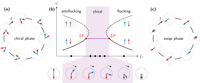
Methods Fig. S1: Bifurcation and phases. (a) Temporal diagram of the chiral phase. (b) Schematic bifurcation diagram of the system along a line at fixed $j_{-}$, for different values of $j_{+}$. (c) Temporal diagram of the swap phase. In the chiral phase (panel a), both populations rotate in the same direction, with the same angular velocity. The direction of rotation is chosen at random. The angle $\Delta\phi^{AB}$ between the velocities of the two populations continuously interpolates between the flocking (where it vanishes) and antiflocking phases (where it is maximal, i.e. equal to $180\mathrm{°}$) along a line connecting them (panel b). In the swap phase (panel c), the velocities oscillate along a fixed direction.

II.1.1 Flocking and antiflocking phase

Let us first look for the conventional, time-independent solutions, by assuming that the polarization eventually converges to a constant, i.e., $\vec{P}^{A(B)}(t)=\vec{P}^{A(B)}_{0}={\rm const.}$ Although, at a glance, it seems possible for the relative angle between $\vec{P}^{A}_{0}$ and $\vec{P}^{B}_{0}$ to take any value, we shall see in the following that it is only possible to be parallel or antiparallel to each other under this assumption, which we call the flocking and antiflocking phase, respectively.

In the time-independent steady state, the mean-field equation (S64) gives

$${\bf 0} = \hat{W}_{0}\left(\begin{array}[]{c}\vec{P}^{A}_{0}\\ \vec{P}^{B}_{0}\end{array}\right)=\left(\begin{array}[]{cc}W^{AA}_{0}&W^{AB}_{0}\\ W^{BA}_{0}&W^{BB}_{0}\end{array}\right)\left(\begin{array}[]{c}\vec{P}^{A}_{0}\\ \vec{P}^{B}_{0}\end{array}\right)$$ (S73)

$$= \left(\begin{array}[]{cc}\eta-j_{AA}\rho^{A}+\frac{1}{2\eta}\big{\lVert}\vec{Q}^{A}_{0}\big{\rVert}^{2}&-j_{AB}\rho^{A}\\ -j_{BA}\rho^{B}&\eta-j_{BB}\rho^{B}+\frac{1}{2\eta}\big{\lVert}\vec{Q}^{B}_{0}\big{\rVert}^{2}\end{array}\right)\left(\begin{array}[]{c}\vec{P}^{A}_{0}\\ \vec{P}^{B}_{0}\end{array}\right),$$ (S78)

with

$$\vec{Q}^{A}_{0}=j_{AA}\vec{P}^{A}_{0}+j_{AB}\vec{P}^{B}_{0},$$ (S79a)

$$\vec{Q}^{B}_{0}=j_{BA}\vec{P}^{A}_{0}+j_{BB}\vec{P}^{B}_{0}.$$ (S79b)

Diagonalizing this matrix $\hat{W}_{0}$ in Eq. (S78) gives

$${\bf 0}=\left(\begin{array}[]{cc}\Gamma_{-}&0\\ 0&\Gamma_{+}\end{array}\right)\left(\begin{array}[]{c}\vec{P}^{-}_{0}\\ \vec{P}^{+}_{0}\end{array}\right).$$ (S84)

Here, the eigenvalues $\Gamma_{\pm}$ roughly correspond to the decay rate of the eigenmodes, where their explicit expressions are given by

$$\Gamma_{\pm} = \frac{1}{2}[W^{AA}_{0}+W^{BB}_{0}\pm\sqrt{\Lambda_{0}}],$$ (S85)

$$\Lambda_{0} = (W^{AA}_{0}-W^{BB}_{0})^{2}+4W^{AB}_{0}W^{BA}_{0},$$ (S86)

with the corresponding eigenmodes,

$${\bf u_{-}}=\left(\begin{array}[]{c}\frac{\sqrt{\Lambda_{0}}-(W^{AA}_{0}-W^{BB}_{0})}{2}\\ -W^{BA}_{0}\end{array}\right),$$ (S87c)

$${\bf u_{+}}=\left(\begin{array}[]{c}W^{AB}_{0}\\ \frac{\sqrt{\Lambda_{0}}-(W^{AA}_{0}-W^{BB}_{0})}{2}\end{array}\right).$$ (S87f)

The order parameter of the flocking phase is transformed accordingly into

$$\left(\begin{array}[]{c}\vec{P}^{-}_{0}\\ \vec{P}^{+}_{0}\end{array}\right)=\hat{U}_{0}\left(\begin{array}[]{c}\vec{P}^{A}_{0}\\ \vec{P}^{B}_{0}\end{array}\right)=\frac{1}{{\rm det}\hat{U}_{0}^{-1}}\left(\begin{array}[]{cc}\frac{\sqrt{\Lambda_{0}}-(W^{AA}_{0}-W^{BB}_{0})}{2}&-W_{0}^{AB}\\ W^{BA}_{0}&\frac{\sqrt{\Lambda_{0}}-(W^{AA}_{0}-W^{BB}_{0})}{2}\end{array}\right)\left(\begin{array}[]{c}\vec{P}^{A}_{0}\\ \vec{P}^{B}_{0}\end{array}\right),$$ (S96)

where $\hat{U}_{0}^{-1}=(\bf u_{-},\bf u_{+})$, or inversely,

$$\left(\begin{array}[]{c}\vec{P}^{A}_{0}\\ \vec{P}^{B}_{0}\end{array}\right)=\left(\begin{array}[]{cc}[U_{0}^{-1}]^{A-}&[U_{0}^{-1}]^{A+}\\ {}[U_{0}^{-1}]^{B-}&[U_{0}^{-1}]^{B+}\end{array}\right)\left(\begin{array}[]{c}\vec{P}^{-}_{0}\\ \vec{P}^{+}_{0}\end{array}\right)=\left(\begin{array}[]{cc}\frac{\sqrt{\Lambda_{0}}-(W^{AA}_{0}-W^{BB}_{0})}{2}&W^{AB}_{0}\\ -W^{BA}_{0}&\frac{\sqrt{\Lambda_{0}}-(W^{AA}_{0}-W^{BB}_{0})}{2}\end{array}\right)\left(\begin{array}[]{c}\vec{P}^{-}_{0}\\ \vec{P}^{+}_{0}\end{array}\right).$$ (S107)

It can be shown from Eq. (S84) that in addition to a trivial solution $\vec{P}^{-}_{0}=\vec{P}^{+}_{0}=0$ that corresponds to a disordered phase, nontrivial solutions with $(\vec{P}_{0}^{-},\vec{P}_{0}^{+})^{\mathsf{T}}\neq 0$ can always be classified into two types Hanai et al. (2019): solutions that satisfy $(\vec{P}^{-}_{0}\neq 0,\vec{P}^{+}_{0}=0)$ and $(\vec{P}^{-}_{0}=0,\vec{P}^{+}_{0}\neq 0)$, which we call "$-$" and "$+$" solutions, respectively. This is readily seen as follows. Let us assume that $\vec{P}^{-(+)}_{0}\neq 0$. Then, it is necessary for the eigenvalue $\Gamma_{-(+)}$ to vanish in order to satisfy the first (second) line of Eq. (S84). In such case, since the eigenvalue of "$+(-)$" is finite $\Gamma_{+(-)}\neq 0$ as long as $\Gamma_{-}\neq\Gamma_{+}$, $\vec{P}^{+(-)}_{0}$ necessarily vanishes because of the second (first) line of Eq. (S84). Thus, $\vec{P}^{-}_{0}$ and $\vec{P}^{+}_{0}$ cannot be nonzero simultaneously, letting us classify the solutions into two types.

The above property has a direct consequence that the polarization field of $A$ and $B$ agents can only be either parallel or antiparallel in the uniform steady state, which we call the flocking and antiflocking phase, respectively. For example, for the "$-$" solution, polarization fields are given by

$$\vec{P}_{0}^{A} = [U_{0}^{-1}]^{A-}\vec{P}_{0}^{-}=\frac{\sqrt{\Lambda_{0}}-(W^{AA}_{0}-W^{BB}_{0})}{2}\vec{P}_{0}^{-},$$ (S108)

$$\vec{P}_{0}^{B} = [U_{0}^{-1}]^{B-}\vec{P}_{0}^{-}=-W^{BA}_{0}\vec{P}_{0}^{-},$$ (S109)

explicitly showing that $\vec{P}^{A}_{0}$ and $\vec{P}^{B}_{0}$ are either parallel or antiparallel to each other, depending on the relative sign between $[U_{0}^{-1}]^{A-}$ and $[U_{0}^{-1}]^{B-}$.

As mentioned earlier, the eigenvalues $\Gamma_{\pm}$ roughly corresponds to the decay rate of the corresponding modes. The condition $\Gamma_{-(+)}=0$ for the "$-(+)$" solution can be regarded as the defining property of a steady state. Assuming $\Lambda_{0}>0$ (that assures $\Gamma_{\pm}$ to be real), the "$-(+)$" solution is likely to be (un)stable since $0<\Gamma_{+}(\Gamma_{-}<0)$, implying a positive (negative) decay rate of the "$+(-)$" mode, where we have used the relation $\Gamma_{-}<\Gamma_{+}$. This strongly suggest that the "$-$" solution is the solution that would be realized. Indeed, as shown in section III.2.2 from a stability analysis, it can proven that "$+$" solution is always unstable, limiting the possible stable solution to the "$-$" solution.

It is important to emphasize that, for the flocking or antiflocking phase to be realized, it is necessary for $\Lambda_{0}$ to be positive since it requires $\sqrt{\Lambda_{0}}$ to be real such that the state can satisfy the relation $\Gamma_{-}=0$ ($\Gamma_{+}=0$) for "$-(+)$" solution. This condition is assured to be satisfied when the sign of the inter-species coupling is the same, i.e., $j_{AB}j_{BA}>0$ (or equivalently $W^{AB}_{0}W^{BA}_{0}>0$), which includes the reciprocal case, since the first term of Eq. (S86), $(W^{AA}_{0}-W^{BB}_{0})^{2}$, is non-negative.

However, when the inter-species couplings have opposite sign (i.e. $j_{AB}j_{BA}<0$ or $W^{AB}_{0}W^{BA}_{0}<0$), $\Lambda_{0}$ may become negative, hence the eigenvalues can turn imaginary implying the existence of a phase transition to a time-oscillating phase. As we show in the following section, the system indeed exhibits a phase transition to an phase where the direction of the orientation continuously oscillates in time, which we call the chiral phase. The phase transition is driven by the non-Hermitian nature of the matrix $\hat{W}$, which can be seen from the observation that the phase transition point, $\Lambda_{0}=0$ is the point where the two eigenvectors $\bm{u}_{\pm}$ (see Eq. (S87)) coalesce; This is the so-called exceptional point Kato (1984). We will further show in section II.1.3 that this transition can be regarded as a spontaneous PT symmetry breaking discussed in the field of non-Hermitian quantum mechanics.

II.1.2 Chiral phase

Below, we look for solutions with an oscillating polarization field, described by the ansatz,

$$\vec{P}^{A}(t)=R^{A}\left(\begin{array}[]{c}\cos(\Omega t+\phi^{A})\\ \sin(\Omega t+\phi^{A})\end{array}\right),$$ (S110c)

$$\vec{P}^{B}(t)=R^{B}\left(\begin{array}[]{c}\cos(\Omega t+\phi^{B})\\ \sin(\Omega t+\phi^{B})\end{array}\right),$$ (S110f)

with $\Omega$ being the frequency of the oscillation and $R^{A},R^{B}(>0)$ the amplitude of the polarization fields of $A$ and $B$ species, respectively. This solution exhibits a "chiral" motion, in the sense that the direction of the orientation continuously evolves in time (while the amplitude of the polarization remains fixed) implying a collective chiral motion of agents, which is exactly what is observed in our microscopic Vicsek model simulation (Fig. 2d in the main text and SI Movie 1).

We note that, for solutions of the form (S110), the $O(2)$ symmetry of the mean-field system assures that $\hat{W}=\hat{W}_{0}$ does not depend on time. This can be directly checked from the observation that the amplitudes of the vectors $\vec{Q}^{A}(t),\vec{Q}^{B}(t)$ given by Eq. (S66) which shows that the magnitude of the nonlinearity in $W^{AA}_{0}$ and $W^{BB}_{0}$ are time-independent.

We show below that the ansatz (S110) satisfies,

$$\Omega = \Omega_{\pm}=\pm\frac{1}{2}\sqrt{|\Lambda_{0}|},$$ (S111)

$$\Delta\phi^{AB} = \phi^{A}-\phi^{B}=\begin{cases}\arccos\left[+\sqrt{\left|\frac{W_{0}^{2}}{W^{AB}_{0}W^{BA}_{0}}\right|}\right]=\arccos\left[+\sqrt{\left|1-\frac{|\Lambda_{0}|}{|W^{AB}_{0}W^{BA}_{0}|}\right|}\right]&(W_{0}W_{0}^{AB}<0)\\ \arccos\left[-\sqrt{\left|\frac{W_{0}^{2}}{W^{AB}_{0}W^{BA}_{0}}\right|}\right]=\arccos\left[-\sqrt{\left|1-\frac{|\Lambda_{0}|}{|W^{AB}_{0}W^{BA}_{0}|}\right|}\right]&(W_{0}W_{0}^{AB}>0)\end{cases}$$ (S112)

with

$$W^{AA}_{0}=-W^{BB}_{0}\equiv W_{0},\qquad R^{B}=\sqrt{\left|\frac{W_{0}^{BA}}{W_{0}^{AB}}\right|}R^{A},$$ (S113)

and importantly, $\Lambda_{0}<0$. The last condition is satisfied only if $W^{AB}_{0}W^{BA}_{0}<0$, i.e. non-reciprocal coupling with opposite signs.

Two comments are in order. Firstly, the fact that we find two solutions, $\Omega=\Omega_{+}>0$ and $\Omega=\Omega_{-}<0$, indicates the occurrence of a spontaneous chiral ($Z_{2}$) symmetry breaking to a left and right-handed phase, respectively. Secondly, the exceptional point $\Lambda_{0}=0$ with $W_{0}>0(<0)$ is a continuous transition point to the (anti)flocking phase, with $\Delta\phi^{AB}=0(=\pi)$. Noting that $W_{0}$ may switch its sign inside the chiral phase, this implies that the chiral flocking phase lies in between the flocking and antiflocking phase (See Fig. S1b.), which is indeed the case (see also Figs. 2f and g).

The mean-field equation (S64) we wish to solve with the ansatz (S110) takes the form

$$-\Omega R^{A}\sin(\Omega t+\phi^{A}) =-W^{AA}_{0}R^{A}\cos(\Omega t+\phi^{A})-W^{AB}_{0}R^{B}\cos(\Omega t+\phi^{B}),$$ (S114)

$$\Omega R^{A}\cos(\Omega t+\phi^{A}) =-W^{AA}_{0}R^{A}\sin(\Omega t+\phi^{A})-W^{AB}_{0}R^{B}\sin(\Omega t+\phi^{B}),$$ (S115)

$$-\Omega R^{B}\sin(\Omega t+\phi^{B}) =-W^{BA}_{0}R^{A}\cos(\Omega t+\phi^{A})-W^{BB}_{0}R^{B}\cos(\Omega t+\phi^{B}),$$ (S116)

$$\Omega R^{B}\cos(\Omega t+\phi^{B}) =-W^{BA}_{0}R^{A}\sin(\Omega t+\phi^{A})-W^{BB}_{0}R^{B}\sin(\Omega t+\phi^{B}).$$ (S117)

Note that Eqs. (S114) and (S115) (Eqs. (S116) and (S117)) are equivalent. These can be factorized as

$$\tilde{R}^{a}\cos(\Omega t+\tilde{\phi}^{a}) =0,$$ (S118)

$$\tilde{R}^{a}\sin(\Omega t+\tilde{\phi}^{a}) =0,$$ (S119)

where $a=A,B$,

$$(\tilde{R}^{A})^{2} =(-W^{AA}_{0}R^{A}\cos\phi^{A}-W^{AB}_{0}R^{B}\cos\phi^{B}+\Omega R^{A}\sin\phi^{A})^{2}+(W^{AA}_{0}R^{A}\sin\phi^{A}+W^{AB}_{0}R^{B}\sin\phi^{B}+\Omega R^{A}\cos\phi^{A})^{2}$$

$$(\tilde{R}^{B})^{2} =(-W^{BA}_{0}R^{A}\cos\phi^{A}-W^{BB}_{0}R^{B}\cos\phi^{B}+\Omega R^{B}\sin\phi^{B})^{2}+(W^{BA}_{0}R^{A}\sin\phi^{A}+W^{BB}_{0}R^{B}\sin\phi^{B}+\Omega R^{B}\cos\phi^{B})^{2}$$

and $\tilde{\phi}^{A},\tilde{\phi}^{B}$ are real constant numbers determined from the parameters $W_{0}^{ab},R^{a},\phi^{a}$. Equations (S118) and (S119) are satisfied at arbitrary $t$ when $\tilde{R}^{A}=\tilde{R}^{B}=0$.

Let us first determine $\Omega$ by solving $\tilde{R}^{A}=0$. This gives,

$$\Omega = \frac{R^{B}}{R^{A}}W^{AB}_{0}\sin\Delta\phi^{AB}\pm i(W^{AA}_{0}+W^{AB}_{0}\frac{R^{B}}{R^{A}}\cos\Delta\phi^{AB}).$$ (S120)

Since we require the frequency $\Omega$ to be real, we demand the imaginary part of Eq. (S120) to vanish,

$$\Delta\phi^{AB}=\arccos\Big{[}-\frac{W^{AA}_{0}}{W^{AB}_{0}}\frac{R^{A}}{R^{B}}\Big{]}.$$ (S121)

Plugging this back into Eq. (S120), we get

$$\Omega = \Omega_{\pm}=\frac{R^{B}}{R^{A}}W^{AB}_{0}\sin\Delta\phi^{AB}=\pm\frac{R^{B}}{R^{A}}W^{AB}_{0}\sqrt{1-\left(\frac{R^{A}}{R^{B}}\frac{W^{AA}_{0}}{W^{AB}_{0}}\right)^{2}}.$$ (S122)

We can similarly compute for $\Omega$ and $\Delta\phi^{AB}$ by solving $\tilde{R}^{B}=0$, where we get

$$\Delta\phi^{AB} = \arccos\Big{[}-\frac{W^{BB}_{0}}{W^{BA}_{0}}\frac{R^{B}}{R^{A}}\Big{]},$$ (S123)

$$\Omega = \Omega_{\pm}=-\frac{R^{A}}{R^{B}}W^{BA}_{0}\sin\Delta\phi^{AB}=\mp\frac{R^{A}}{R^{B}}W^{BA}_{0}\sqrt{1-\left(\frac{R^{B}}{R^{A}}\frac{W^{BB}_{0}}{W^{BA}_{0}}\right)^{2}}.$$ (S124)

The solution sets given by Eqs. (S121), (S122) and by Eqs. (S123), (S124) should be identical. Noting that $W^{AB}_{0}W^{BA}_{0}<0$ and thus $\Omega_{\pm}$ in Eqs. (S122) and (S124) have the same sign, we get the relation

$$\frac{W^{AA}_{0}}{W^{AB}_{0}}\frac{R^{A}}{R^{B}} = \frac{W^{BB}_{0}}{W^{BA}_{0}}\frac{R^{B}}{R^{A}},$$ (S125)

$$\frac{R^{B}}{R^{A}}W^{AB}_{0}\sqrt{1-\left(\frac{R^{A}}{R^{B}}\frac{W^{AA}_{0}}{W^{AB}_{0}}\right)^{2}} = -\frac{R^{A}}{R^{B}}W^{BA}_{0}\sqrt{1-\left(\frac{R^{B}}{R^{A}}\frac{W^{BB}_{0}}{W^{BA}_{0}}\right)^{2}}.$$ (S126)

Solving the above yields,

$$W^{AA}_{0} = -W^{BB}_{0}\equiv W_{0},$$ (S127)

$$R^{A} = \sqrt{-\frac{W^{AB}_{0}}{W^{BA}_{0}}}R^{B}=\sqrt{\left|\frac{W^{AB}_{0}}{W^{BA}_{0}}\right|}R^{B},$$ (S128)

giving,

$$\Omega_{\pm} = \pm\sqrt{|W^{AB}_{0}W^{BA}_{0}|-W_{0}^{2}}=\pm\frac{\sqrt{|\Lambda_{0}|}}{2},$$ (S129)

and

$$\Delta\phi^{AB} = \arccos\left[\sqrt{\frac{W_{0}^{2}}{|W^{AB}_{0}W^{BA}_{0}|}}\right],$$ (S130)

for $W_{0}W_{0}^{AB}<0$, and for $W_{0}W_{0}^{AB}>0$,

$$\Delta\phi^{AB} = \arccos\left[-\sqrt{\frac{W_{0}^{2}}{|W^{AB}_{0}W^{BA}_{0}|}}\right].$$ (S131)

Hence, we arrive at the relations (S110)-(S112).

II.1.3 The (anti)flocking to chiral phase transition as spontaneous PT symmetry breaking

In this subsection, we show that our system is PT symmetric (in the sense defined below) and the (anti)flocking-to-chiral phase transition can be regarded as an instance of spontaneous PT symmetry breaking, often discussed in the context of non-Hermitian quantum mechanics Bender and Boettcher (1998); Bender (2007); Konotop et al. (2016); Mostafazadeh (2002a, b, c); Bender et al. (2002); Mostafazadeh (2015); Bender and Mannheim (2010). In the following, we consider the operations executed by the operators ${\mathcal{P}}$ and ${\mathcal{T}}$, which are the generalized parity and time-reversal operator, respectively (i.e., they are not necessarily related to the physical parity and time-reversal operations). Here, ${\mathcal{P}}$ is defined to be a generic Hermitian and unitary operator and ${\mathcal{T}}$ is a generic antiunitary operator, expressible as $K$ times a unitary matrix (where $K$ is a complex conjugation) that satisfy

$${\mathcal{P}}^{2}={\mathcal{T}}^{2}=1,\qquad[{\mathcal{P}},{\mathcal{T}}]=0,$$ (S132)

as would the conventional parity and time-reversal operators.

The system is said to be PT symmetric if we can find a ${\mathcal{P}}{\mathcal{T}}$ operator that commutes with the matrix $\hat{W}_{0}$ that controls the dynamics:

$$[{\mathcal{P}}{\mathcal{T}},\hat{W}_{0}]=0.$$ (S133)

The PT symmetry of a PT symmetric system is said to be unbroken if any eigenstate of the matrix $\hat{W}_{0}$ is simultaneously an eigenstate of the ${\mathcal{P}}{\mathcal{T}}$ operator. Otherwise, the PT symmetry is said to be spontaneously broken Konotop et al. (2016).

We argue below that (i) our system is PT symmetric, (ii) the (anti)flocking phase is a PT unbroken phase, and (iii) the chiral phase is a PT broken phase. Hence, the (anti)flocking-to-chiral phase transition is an instance of spontaneous PT symmetry breaking.

Our system is PT symmetric since we can find operators ${\mathcal{P}}$ and ${\mathcal{T}}$ that satisfy Eq. (S133). To see this explicitly, following Ref. Mostafazadeh (2002a), we express the matrix $\hat{W}_{0}$ and the operators ${\mathcal{P}}$ and ${\mathcal{T}}$ in terms of Pauli matrices,

$$\hat{W}_{0} = w_{0}^{0}\bm{1}+\bm{w}_{0}\cdot\bm{\sigma}$$ (S134)

$${\mathcal{P}} = p^{0}\bm{1}+\bm{p}\cdot\bm{\sigma},$$ (S135)

$${\mathcal{T}} = K\sigma_{2}(t^{0}\bm{1}+\bm{t}\cdot\bm{\sigma}),$$ (S136)

where $\bm{\sigma}=(\sigma_{1},\sigma_{2},\sigma_{3})^{\mathsf{T}}$ is a vector composed of Pauli matrices. From their definitions introduced above, the vectors $\bm{p}$ and $\bm{t}$ need to be real with

$$p^{0}=t^{0}=0,\bm{p}\cdot\bm{p}=\bm{t}\cdot\bm{t}=1,\bm{p}\cdot\bm{t}=0.$$ (S137)

Further decomposing the vector $\bm{w}_{0}$ into real and imaginary part as $\bm{w}_{0}=\bm{w}_{0}^{R}+i\bm{w}_{0}^{I}$, we find Mostafazadeh (2002a)

$${\mathcal{P}}{\mathcal{T}}\hat{W}_{0}({\mathcal{P}}{\mathcal{T}})^{-1}-\hat{W}_{0}=2\bm{\sigma}\cdot\bm{F}-2i\bm{\sigma}\cdot\bm{G}$$ (S138)

where

$$\bm{F} = (\bm{w}_{0}^{R}\cdot\bm{p})\bm{p}+(\bm{w}_{0}^{R}\cdot\bm{t})\bm{t}-\bm{w}_{0}^{R},$$ (S139)

$$\bm{G} = (\bm{w}_{0}^{I}\cdot\bm{p})\bm{p}+(\bm{w}_{0}^{I}\cdot\bm{t})\bm{t}.$$ (S140)

The existence of $\bm{p}$ and $\bm{t}$ that makes the right-hand side of Eq. (S138) vanish means that the system is PT symmetric.

We can indeed find such $\bm{p}$ and $\bm{t}$ for our system, by using the property that $\hat{W}_{0}$ is a real matrix that restrict $w_{0}^{0}$ to be real and the real vectors $\bm{w}_{0}^{R},\bm{w}_{0}^{I}$ to take the form $\bm{w}_{0}^{R}=(w_{0}^{1},0,w_{0}^{3})^{\mathsf{T}}$ and $\bm{w}_{0}^{I}=(0,w_{0}^{2},0)^{\mathsf{T}}$. Thus,

$$\bm{w}_{0}^{R}\cdot\bm{w}_{0}^{I}=0.$$ (S141)

By choosing

$$\bm{p}=\frac{\bm{w}_{0}^{R}}{|\bm{w}_{0}^{R}|},$$ (S142)

since $\bm{p}\cdot\bm{t}=0$, we get $\bm{w}_{0}^{R}\cdot\bm{t}=0$. Plugging these into Eq. (S139) yields $\bm{F}=0$. Further, since $\bm{p}\propto\bm{w}_{0}^{R}$, Eq. (S141) gives

$$\bm{p}\cdot\bm{w}_{0}^{I}=0,$$ (S143)

leading to $\bm{G}=(\bm{w}_{0}^{I}\cdot\bm{t})\bm{t}$. Since $\bm{w}_{0}^{I}$ and $\bm{t}$ are in a plane orthogonal to $\bm{p}$, we can always find $\bm{t}$ that are also orthogonal to $\bm{w}_{0}^{I}$. Choosing such a vector $\bm{t}$, i.e.,

$$\bm{t}=\frac{\bm{w}_{0}^{R}\times\bm{w}_{0}^{I}}{|\bm{w}_{0}^{R}\times\bm{w}_{0}^{I}|},$$ (S144)

we get $\bm{G}=0$ and therefore the right-hand side of Eq. (S138) vanishes. Thus, our system is PT symmetric.

Now we argue that the flocking and antiflocking phases are in a PT unbroken phase while the chiral phase is in a PT broken phase. In a PT symmetric system, the eigenstates $\bm{u}_{\pm}$, defined as states that satisfies

$$\hat{W}_{0}\bm{u}_{\pm}=\Gamma_{\pm}\bm{u}_{\pm},$$ (S145)

also satisfies

$$\hat{W}_{0}({\mathcal{P}}{\mathcal{T}}\bm{u}_{\pm})=\Gamma_{\pm}^{*}({\mathcal{P}}{\mathcal{T}}\bm{u}_{\pm}),$$ (S146)

showing that ${\mathcal{P}}{\mathcal{T}}\bm{u}_{\pm}$ is also an eigenstate of this system. Here, we have operated ${\mathcal{P}}{\mathcal{T}}$ from the left and used Eq. (S133).

In a PT unbroken phase, since ${\mathcal{P}}{\mathcal{T}}\bm{u}_{\pm}\propto\bm{u}_{\pm}$ and thus satisfies

$$\hat{W}_{0}\bm{u}_{\pm}=\Gamma_{\pm}^{*}\bm{u}_{\pm},$$ (S147)

the eigenvalues of PT unbroken phase is real ($\Gamma_{\pm}=\Gamma_{\pm}^{*}$). On the other hand, in a PT broken phase, ${\mathcal{P}}{\mathcal{T}}\bm{u}_{+(-)}$ is a distinct vector from $\bm{u}_{+(-)}$. Thus, the eigenstate with the eigenvalue $\Gamma_{+(-)}^{*}$ is a different state from that with $\Gamma_{+(-)}$. Since there are at most two eigenvalues in our two component system, the two eigenvalues are complex conjugate of each other,

$$\Gamma_{+}=\Gamma_{-}^{*}.$$ (S148)

While the flocking and antiflocking phase corresponds to real eigenvalues, the chiral phase corresponds to complex eigenvalues that are complex conjugate of each other, resulting in an oscillation in time. Hence, the former is in a PT unbroken phase while the latter is in a PT broken phase, marking the phase transition point as a PT symmetry breaking point.

II.2 Mean-field phase diagram

So far, we have observed how the flocking/antiflocking phase may be destabilized into a chiral phase, without paying too much attention to the concrete form of the matrix $\hat{W}_{0}$. Here, we directly compute analytically the mean-field equation (S64) to show that the flocking, antiflocking, and the chiral phase predicted from the above analysis indeed arise. We determine the phase diagram in terms of the microscopic coupling strengths $j_{ab}(a,b=A,B)$.

Below, we parameterize

$$j_{\pm} = \frac{1}{2}(j_{AB}\pm j_{BA}),$$ (S149)

for our convenience, where $j_{+}$ and $j_{-}$ characterize the reciprocal and non-reciprocal component of the coupling, respectively.

II.2.1 Ordered-to-disordered phase transition

Firstly, we analyze the ordered-to-disordered phase transition point within mean-field approximation. Starting from the ordered phase (i.e. flocking and antiflocking phase), the order parameter $\vec{P}_{0}^{a}$ approaches zero as moving towards the phase boundary. Thus, the ordered-to-disordered phase transition point should satisfy,

$${\rm det}\hat{W}_{0}(\vec{P}^{A}_{0}\rightarrow 0,\vec{P}^{B}_{0}\rightarrow 0)=\Gamma_{-}(\vec{P}^{A}_{0}\rightarrow 0,\vec{P}^{B}_{0}\rightarrow 0)\Gamma_{+}(\vec{P}^{A}_{0}\rightarrow 0,\vec{P}^{B}_{0}\rightarrow 0)=0.$$ (S150)

This can be solved analytically with the result (For simplicity, we assume below $\rho^{A}=\rho^{B}=\rho$.),

$$j_{+}^{c}=\pm\frac{\sqrt{\eta^{2}-\eta(j_{AA}+j_{BB})\rho+(j_{AA}j_{BB}+j_{-}^{2})\rho^{2}}}{\rho}.$$ (S151)

Note that, as discussed earlier, the ordered phase should be described as the stable "$-$" solution and not the unstable "$+$" solution. While the "$-$" solution satisfies $\Gamma_{-}=0,\Gamma_{+}>0$, the "$+$" solution satisfies $\Gamma_{-}<0,\Gamma_{+}=0$. Thus, the sign of the average $(\Gamma_{+}+\Gamma_{-})/2$ indicates which type the obtained solution is. Since

$$\Gamma_{\pm}(\vec{P}^{A}_{0}\rightarrow 0,\vec{P}^{B}_{0}\rightarrow 0)=-\frac{1}{2}[(j_{AA}+j_{BB})\rho-2\eta\pm\sqrt{\Lambda_{0}}],$$ (S152)

the average of the two eigenvalues are given by

$$\frac{\Gamma_{+}+\Gamma_{-}}{2}=-\frac{1}{2}\big{[}(j_{AA}+j_{BB})\rho-2\eta\big{]}.$$ (S153)

Thus, Eq. (S151) is valid only when

$$\eta>(j_{AA}+j_{BB})\rho$$ (S154)

is satisfied such that it describes the destabilization towards the stable "$-$" solution. We have drawn this ordered-to-disordered phase boundary in Fig. 2a in the main text (black line), giving an excellent agreement with the numerical result.

II.2.2 Exceptional point

We next determine the exceptional point that marks the exceptional transition point from the (anti)flocking to a chiral phase for a given parameter set $(\rho^{A},\rho^{B},j_{AA},j_{BB})$. At the transition point, the following relations are satisfied:

$$\Gamma_{-} = \bar{W}_{0}-\frac{\sqrt{\Lambda}_{0}}{2}=0,$$ (S155)

$$\Lambda_{0} = (\Delta W_{0})^{2}+4W_{0}^{AB}W_{0}^{BA}=0,$$ (S156)

$$R^{A} = \left|\frac{\sqrt{\Lambda}_{0}-\Delta W_{0}}{2W_{0}^{BA}}\right|R^{B},$$ (S157)

where $R^{a}=\big{\lVert}\vec{P}^{a}_{0}\big{\rVert}(>0)$,

$$\bar{W}_{0} = \frac{W_{0}^{AA}+W_{0}^{BB}}{2}=-\frac{1}{2}\big{[}(j_{AA}+j_{BB})\rho-2\eta-\frac{1}{2\eta}(\big{\lVert}\vec{Q}^{A}_{0}\big{\rVert}^{2}+\big{\lVert}\vec{Q}^{B}_{0}\big{\rVert}^{2})\big{]},$$ (S158)

$$\Delta W_{0} = \frac{W_{0}^{AA}-W_{0}^{BB}}{2}=-\frac{1}{2}\big{[}(j_{AA}-j_{BB})\rho-2\eta-\frac{1}{2\eta}(\big{\lVert}\vec{Q}^{A}_{0}\big{\rVert}^{2}-\big{\lVert}\vec{Q}^{B}_{0}\big{\rVert}^{2})\big{]},$$ (S159)

with

$$\big{\lVert}\vec{Q}^{A}_{0}\big{\rVert}^{2} = \big{\lVert}j_{AA}\vec{P}_{0}^{A}+j_{AB}\vec{P}_{0}^{B}\big{\rVert}^{2},$$ (S160)

$$\big{\lVert}\vec{Q}^{B}_{0}\big{\rVert}^{2} = \big{\lVert}j_{BA}\vec{P}_{0}^{A}+j_{BB}\vec{P}_{0}^{B}\big{\rVert}^{2}.$$ (S161)

Here, Eq. (S155) is the steady state condition, Eq. (S156) is condition for the exceptional point, and Eq. (S157) is derived from Eqs. (S108) and (S109). Eq. (S156) shows that non-reciprocal interaction with $W_{0}^{AB}W_{0}^{BA}<0$ (hence $j_{AB}j_{BA}<0$) is necessary for the chiral flocking phase to appear. Below, we assume without loss of generality that the interaction are non-reciprocal with opposite sign, i.e. $j_{AB}j_{BA},W_{0}^{AB}W_{0}^{BA}<0$.

From Eqs. (S155) and (S156),

$$\Delta W_{0}=\pm 2\sqrt{|W_{0}^{AB}W_{0}^{BA}|}.$$ (S162)

Plugging this into Eq. (S157), we get

$$R_{B}=\sqrt{\left|\frac{W_{0}^{BA}}{W_{0}^{AB}}\right|}R_{A}=\sqrt{\left|\frac{j_{BA}\rho^{B}}{j_{AB}\rho^{A}}\right|}R_{A}.$$ (S163)

For the flocking phase,

$$\big{\lVert}\vec{Q}^{A}_{0}\big{\rVert}^{2} = (j_{AA}R_{A}+j_{AB}R_{B})^{2},$$ (S164)

$$\big{\lVert}\vec{Q}^{B}_{0}\big{\rVert}^{2} = (j_{BA}R_{A}+j_{BB}R_{B})^{2},$$ (S165)

while for the antiflocking phase,

$$\big{\lVert}\vec{Q}^{A}_{0}\big{\rVert}^{2} = (j_{AA}R_{A}-j_{AB}R_{B})^{2},$$ (S166)

$$\big{\lVert}\vec{Q}^{B}_{0}\big{\rVert}^{2} = (j_{BA}R_{A}-j_{BB}R_{B})^{2}.$$ (S167)

We solve the coupled equations

$$\bar{W}_{0} = 0,$$ (S168)

Eq. (S162), and Eq. (S163) for $R_{A},R_{B}$ and the critical value $j_{+}^{EP}$ for a given $j_{-}$.

We can solve the above equations analytically in the case $j_{AA}=j_{BB}(\equiv j)$, as we perform in the following. We only consider here the flocking-to-chiral phase transition point, as the antiflocking-chiral transition point can be computed in a similar way. Using Eq. (S163) to eliminate $R_{B}$, Eq. (S162) yields the relation

$$R_{A}^{2}=\frac{4\eta j_{AB}\sqrt{-j_{AB}j_{BA}}\rho}{2jj_{AB}(j_{AB}-j_{BA})\sqrt{-j_{BA}/j_{AB}}+j^{2}(j_{AB}+j_{BA})-j_{AB}j_{BA}(j_{AB}+j_{BA})}.$$ (S169)

We substitute this to Eq. (S168) to get,

$$\begin{split}(j^{2}+j_{AB}j_{BA})\big{[}j(j_{AB}+j_{BA})+\sqrt{-j_{AB}j_{BA}}(j_{AB}-j_{BA})\big{]}\rho\\ =\big{[}(j^{2}-j_{AB}j_{BA})(j_{AB}+j_{BA})+2j\sqrt{-j_{AB}j_{BA}}(j_{AB}-j_{BA})\big{]}\eta.\end{split}$$ (S170)

This can be rewritten in terms of $j_{\pm}$ introduced in Eq. (S149),

$$(j^{2}+j_{+}^{2}-j_{-}^{2})(jj_{+}+j_{-}\sqrt{j_{-}^{2}-j_{+}^{2}})\rho=(2jj_{-}\sqrt{j_{-}^{2}-j_{+}^{2}}+j_{+})(jj_{+}+j_{-}\sqrt{j_{-}^{2}-j_{+}^{2}})\eta,$$ (S171)

which can be organized into a cubic equation in terms of $j_{+}^{2}$ as,

$$aj_{+}^{6}+bj_{+}^{4}+cj_{+}^{2}+d=0$$ (S172)

with

$$a = (\eta+j\rho)^{2}+j_{-}^{2}\rho^{2},$$ (S173)

$$b = 2j^{4}\rho^{2}-2\eta^{2}(j^{2}-j_{-}^{2})-8\eta jj_{-}^{2}-3j_{-}^{4}\rho^{2},$$ (S174)

$$c = \eta^{2}j^{4}+6\eta^{2}j^{2}j_{-}^{2}+\eta^{2}j_{-}^{4}-2\eta j^{5}\rho-4\eta j^{3}j_{-}^{2}\rho+10\eta jj_{-}^{4}\rho+j^{6}\rho^{2}-j^{4}j_{-}^{2}\rho^{2}-3j^{2}j_{-}^{4}\rho^{2}+3j_{-}^{6}\rho^{2},$$ (S175)

$$d = j_{-}^{4}[-4\eta^{2}j^{2}(1+j\rho)-j^{4}\rho^{2}-4\eta j\rho j_{-}^{2}+2j^{2}\rho^{2}j_{-}^{2}-\rho^{2}j_{-}^{4}].$$ (S176)

This can be solved exactly using Cardano’s formula. Its real solution is plotted as a red line in Figs. 2b and 2c in the main text, giving an excellent agreement with the (anti)flocking/chiral phase transition lines obtained numerically.

III Excitation spectrum and stability analysis

In this section, we provide a linear analysis on the fluctuations around the mean-field solution obtained in section II to study the properties of excitations, the stability of the phases described above, as well as the nature of the phase transitions between them. We confirm that there is a wide range of parameters where the flocking, antiflocking, and chiral phases are stable, as summarized in the phase diagram in Fig. 3a in the main text.

We show from this analysis that the chiral phase emerges by the coalescence of the collective eigenmodes in the transverse channel, which is a fundamentally different mechanism from the conventional phase transition scenarios Hanai and Littlewood (2020). We further show that the emergence of the swap phase can be understood as the instability of the flocking/antiflocking phase against the global longitudinal fluctuations. Based on these results, we argue that it leads to the appearance of chiral-swap mixed phase exhibiting quasiperiodic oscillation in time, and explain the occurrence of tetracritical points with reduced codimension in the phase diagram. We also describe how the combination of exceptional points and the convective terms enforces the occurrence of the pattern-forming instabilities at the (anti)flocking-to-chiral phase transition.

III.1 General considerations

We assume the existence of a homogeneous solution $\psi(t)=(\rho_{a}(t),P_{a}(t))_{a}$ to the equation (S51), which therfore also satisfies the mean-field Eq. (S64). This equation is of the form

$$\partial_{t}\psi(t,r)=f(\psi(t,r),\nabla\psi(t,r),\dots)$$ (S177)

The linear stability and the fate of small excitations (e.g. waves) on top of the steady-state are ruled by the linearized equation of motion for small perturbations $\delta\psi=\psi-\psi_{\text{ss}}$ on top of a steady-state $\psi_{\text{ss}}$. At first order in $\delta\psi$, the perturbations are described by the equation

$$\partial_{t}\delta\psi(t,r)=f(\psi(t,r),\nabla\psi(t,r),\dots)-f(\psi_{\text{ss}}(t),\nabla\psi_{\text{ss}}(t)\equiv 0,\dots)\simeq\hat{\mathcal{L}}(t)\delta\psi(t,r)+\mathcal{O}(\delta\psi^{2})$$ (S178)

where $\hat{\mathcal{L}}(t)$ is a linear (differential) operator, that may depend on time through the steady-state $\psi_{\text{ss}}(t)$. As this operator is linear, we use the Fourier transform to block-diagonalize the differential operators in momentum space, where we are left with a family of linear equations of the form

$$\partial_{t}\delta\psi(t,k)=\mathcal{L}(t,k)\delta\psi(t,k)$$ (S179)

where $\mathcal{L}(t,k)$ are finite matrices. In terms of the perturbations $\delta P^{a}_{\mu}$ and $\delta\rho^{a}$ of the polarization fields and density fields,

$$\partial_{t}\delta P^{a}_{\mu} =[\mathcal{L}_{PP}]^{ab}_{\mu\nu}\delta P^{b}_{\nu}+[\mathcal{L}_{P\rho}]^{ab}_{\mu}\delta\rho^{b}$$ (S180a)

$$\partial_{t}\delta\rho^{a} =[\mathcal{L}_{\rho\rho}]^{ab}\delta\rho^{b}+[\mathcal{L}_{\rho P}]^{ab}_{\nu}\delta P^{b}_{\nu}.$$ (S180b)

Hence, the matrix elements of $\mathcal{L}$ are

$$\begin{split}[\mathcal{L}_{PP}]^{ab}_{\mu\nu}=-D_{\theta}\delta_{ab}\delta_{\mu\nu}+j_{ab}\rho^{a}\delta_{\mu\nu}-\frac{1}{2D_{\theta}}\sum_{c,d,\rho}j_{ac}j_{ad}P^{c}_{\rho}P^{d}_{\rho}\delta_{ab}\delta_{\mu\nu}-\frac{1}{D_{\theta}}\sum_{c}j_{ab}j_{ac}P^{a}_{\mu}P^{c}_{\nu}\\ +D_{a}(-k^{2})\delta_{ab}\delta_{\mu\nu}\\ +\sum_{c}\lambda_{ac}\Big{[}-\text{i}k_{\rho}P^{c}_{\rho}\delta_{ab}\delta_{\mu\nu}+3\text{i}k_{\mu}P^{c}_{\nu}\delta_{ab}-3P^{c}_{\mu}\text{i}k_{\nu}\delta_{ab}\Big{]}\\ +\lambda_{ab}\Big{[}-2P^{a}_{\mu}\text{i}k_{\nu}+2\text{i}k_{\mu}P^{a}_{\nu}-2P^{a}_{\rho}\text{i}k_{\rho}\delta_{\mu\nu}\Big{]}\end{split}$$ (S181)

and

$$[\mathcal{L}_{P\rho}]^{ab}_{\mu} =\left[(\sum_{c}j_{ac}P^{c})-\frac{v_{0}^{a}}{2}\text{i}k\right]\delta_{ab}$$ (S182)

$$[\mathcal{L}_{\rho P}]^{ab}_{\mu} =-\delta_{ab}v_{0}^{b}\text{i}k_{\mu}$$ (S183)

$$[\mathcal{L}_{\rho\rho}]^{ab} =0.$$ (S184)

In the following, we neglect density fluctuations, setting $\delta\rho_{a}=0$. Hence, we will only consider the stability of the polarization channel described by $\hat{L}=\mathcal{L}_{PP}$. This can happen, for instance, when the system is incompressible (see Refs. Chen et al. (2015, 2018) for an analysis of the consequences in the Toner-Tu model for a single population). Here, we do not impose the divergence constraint $\operatorname{div}(\vec{v}_{a})=0$ that would usually arise from the continuity equation by integrating out high-frequency density fluctuations; instead, we assume that the continuity equation includes appropriate source terms so that density fluctuations can be traced out without producing constraints on the velocities. We refer to section XI for a discussion of the situation in which the incompressibility constraint is imposed.

III.2 Stability of the flocking/antiflocking phase

We start with the stability analysis on the flocking and the antiflocking phase. In these phases, the steady state solutions can be written as

$$\vec{P}^{a}_{0}=P^{a}_{0}\;\vec{e}_{\sslash}.$$ (S185)

for $a=A,B$, where $P_{0}^{a}$ are real numbers and $\vec{e}_{\sslash}$ is a unit vector pointing at the flocking direction. Crucially $\vec{e}_{\sslash}$ is the same for $a=A$ and $a=B$. With this notation, $P^{A}_{0}P^{B}_{0}>0\,(<0)$ corresponds to the (anti)flocking phase. It is convenient to decompose the fluctuations into longitudinal ($\sslash$) and transverse ($\perp$) components,

$$\delta\vec{P}^{a}(\bm{r},t)=\vec{e}_{\sslash}\delta P^{a}_{\sslash}(\bm{r},t)+\vec{e}_{\perp}\delta P^{a}_{\perp}(\bm{r},t)=P^{a}_{0}\big{[}\vec{e}_{\sslash}\delta n^{a}(\bm{r},t)+\vec{e}_{\perp}\delta\phi^{a}(\bm{r},t)\big{]},$$ (S186)

where $\vec{e}_{\perp}$ is a unit vector perpendicular to the flocking direction $\vec{e}_{\sslash}$. In this way, $\delta n^{a}$ represents longitudinal fluctuations normalized by $P_{0}^{a}$, and $\delta\phi^{a}$ is the angle describing the deviation from the flocking direction.

The relevant part of the linearized version (S179) of the coupled Toner-Tu equations (S62) then reads, in Fourier space,

$$\hat{L}(\bm{k})d\vec{y}(\bm{k})=s(\bm{k})d\vec{y}(\bm{k}),$$ (S187)

where $\bm{k}=k_{\sslash}\vec{e}_{\sslash}+k_{\perp}\vec{e}_{\perp}$, $\hat{L}=\mathcal{L}_{PP}$ as defined in (S181),

$$d\vec{y}(\bm{k})=\left(\begin{array}[]{c}\delta\phi^{A}(\bm{k})\\ \delta\phi^{B}(\bm{k})\\ \delta n^{A}(\bm{k})\\ \delta n^{B}(\bm{k})\end{array}\right),$$ (S192)

and $\omega(\bm{k})$ is the dispersion relation of a collective mode. We decompose the 4x4 matrix $\hat{L}(\bm{k})$ controlling the linear excitations of the system as the block matrix

$$\hat{L}(\bm{k})=\left(\begin{array}[]{cc}\hat{L}_{\perp\perp}(\bm{k})&\hat{L}_{\perp\sslash}(\bm{k})\\ \hat{L}_{\sslash\perp}(\bm{k})&\hat{L}_{\sslash\sslash}(\bm{k})\end{array}\right),$$ (S195)

where the blocks correspond to the transverse and longitudinal channels (blocks on the diagonal) and their coupling (off-diagonal). They have the explicit form

$$\hat{L}_{\perp\perp}(\bm{k}) =-\left(\begin{array}[]{cc}W^{AA}_{0}&\frac{W^{AB}_{0}P^{B}_{0}}{P^{A}_{0}}\\ \frac{W^{BA}_{0}P^{A}_{0}}{P^{B}_{0}}&W^{BB}_{0}\end{array}\right)-i\hat{\lambda}^{\perp\perp}k_{\sslash}-\left(\begin{array}[]{cc}D_{0}^{A}&0\\ 0&D_{0}^{B}\end{array}\right)\bm{k}^{2},$$ (S196e)

$$\hat{L}_{\perp\sslash}(\bm{k}) =i\hat{\lambda}^{\perp\sslash}k_{\perp},$$ (S196f)

$$\hat{L}_{\sslash\perp}(\bm{k}) =-i\hat{\lambda}^{\sslash\perp}k_{\perp},$$ (S196g)

$$\hat{L}_{\sslash\sslash}(\bm{k}) =-\left(\begin{array}[]{cc}W^{AA}_{0}&\frac{W^{AB}_{0}P^{B}_{0}}{P^{A}_{0}}\\ \frac{W^{BA}_{0}P^{A}_{0}}{P^{B}_{0}}&W^{BB}_{0}\end{array}\right)-\left(\begin{array}[]{cc}\frac{j^{AA}}{\eta}P_{0}^{A}{Q}^{A}_{0}&\frac{j^{AB}}{\eta}P_{0}^{B}{Q}^{A}_{0}\\ \frac{j^{BA}}{\eta}P_{0}^{A}{Q}^{B}_{0}&\frac{j^{BB}}{\eta}P_{0}^{B}{Q}^{B}_{0}\end{array}\right)-i\hat{\lambda}^{\sslash\sslash}k_{\sslash}-\left(\begin{array}[]{cc}D_{0}^{A}&0\\ 0&D_{0}^{B}\end{array}\right)\bm{k}^{2},$$ (S196n)

where

$${Q}^{A}_{0}=j_{AA}P^{A}_{0}+j_{AB}P^{B}_{0},$$ (S197a)

$${Q}^{B}_{0}=j_{BA}P^{A}_{0}+j_{BB}P^{B}_{0},$$ (S197b)

and $\hat{\lambda}^{\perp\perp},\hat{\lambda}^{\perp\sslash},\hat{\lambda}^{\sslash\perp}$, and $\hat{\lambda}^{\sslash\sslash}$ are 2$\times$2 real matrices that originate from the convective terms, given by

$$\hat{\lambda}^{\perp\perp}=\hat{\lambda}^{\sslash\sslash} = \begin{pmatrix}3P^{A}_{0}\lambda_{AA}+P^{B}_{0}\lambda_{AB}&2P^{B}_{0}\lambda_{AB}\\ 2P^{A}_{0}\lambda_{BA}&P^{A}_{0}\lambda_{BA}+3P^{B}_{0}\lambda_{BB}\end{pmatrix},$$ (S198)

$$\hat{\lambda}^{\perp\sslash}=\hat{\lambda}^{\sslash\perp} = \begin{pmatrix}5P^{A}_{0}\lambda_{AA}+3P^{B}_{0}\lambda_{AB}&2P^{B}_{0}\lambda_{AB}\\ 2P^{A}_{0}\lambda_{BA}&3P^{A}_{0}\lambda_{BA}+5P^{B}_{0}\lambda_{BB}\end{pmatrix}.$$ (S199)

We use

$$D_{a}=\frac{(v_{0}^{a})^{2}}{16\eta}\qquad\lambda_{ab}=v_{0}^{a}v_{0}^{b}$$ (S200)

in our analysis (see section I for further discussion on this point).

III.2.1 Computation of the stability regions of the phase diagram

We determine the regions of stability of the (anti)flocking phases (Fig. 3a of the main text) by first solving numerically the mean-field dynamical system in Eq. (S64) to obtain the quantities $R_{a}=\lVert\vec{P}_{a}\rVert$ ($a=A,B$) and $\Delta\phi^{AB}=\text{angle}(\vec{P}_{A},\vec{P}_{B})$. This allows to identify the phase, and to obtain the matrix $\hat{L}(k)$ using Eq. (S181). The eigenvalues $s_{\alpha}(k)=\sigma_{\alpha}(k)+\text{i}\omega_{\alpha}(k)$ of this matrix give the growth rates $\sigma_{\alpha}(k)$ and the frequencies $\omega_{\alpha}(k)$ of the perturbations. Because of the existence of a Goldstone mode, the largest growth rate is pinned to $\sigma=0$ at $k=0$. To evaluate the stability of the phase, we determine whether $k=0$ is a local maximum by computing the sign of the eigenvalues of the Hessian matrix of $\sigma(k)$ at $k=0$, which is obtained by discretizing the second derivatives in momentum space. The result is presented in Fig. 3a of the main text. We have verified manually (by directly computing the growth rates as a function of $k$) that for a large range of parameters, an instability is present only if $k=0$ is not a local minimum. However, this hypothesis might fail in particular cases. This shortcoming will be addressed in future works by determining the stability regions directly from the full momentum dependent growth rates. The largest growth rates as a function of the wavevector in Fig. 4b are directly obtained by diagonalizing $\hat{L}(k)$ at each point.

III.2.2 Goldstone’s theorem and destabilization towards the chiral phase

Since the flocking and antiflocking phase are spontaneous symmetry broken phases, Goldstone’s theorem assures that at least one gapless eigenmode (i.e. the Goldstone mode) exists Altland and Simons (2010). This can be shown explicitly as follows. Using the steady state mean-field equation (S78), or

$$W^{AA}_{0} = -\frac{W^{AB}_{0}P^{B}_{0}}{P^{A}_{0}}=\frac{j^{AB}\rho^{A}P^{B}_{0}}{P^{A}_{0}},$$ (S201)

$$W^{BB}_{0} = -\frac{W^{BA}_{0}P^{A}_{0}}{P^{B}_{0}}=\frac{j^{BA}\rho^{B}P^{A}_{0}}{P^{B}_{0}},$$ (S202)

the transverse-transverse block of the dynamical matrix $\hat{L}$ at $\bm{k}=0$ can be simplified to

$$\hat{L}_{\perp\perp}(\bm{k}={\bf 0})=-\left(\begin{array}[]{cc}W^{AA}_{0}&-W^{AA}_{0}\\ -W^{BB}_{0}&W^{BB}_{0}\end{array}\right).$$ (S205)

Then, it is readily shown, by noting that the transverse and the longitudinal fluctuations decouple at $\bm{k}={\bf 0}$ since $\hat{L}_{\perp\sslash}(\bm{k}={\bf 0})=L_{\sslash\perp}(\bm{k}={\bf 0})=0$, that the vector

$$d\vec{y}(\bm{k}={\bf 0})=\left(\begin{array}[]{c}\delta\phi^{A}({\bf 0})\\ \delta\phi^{B}({\bf 0})\\ \delta n^{A}({\bf 0})\\ \delta n^{B}({\bf 0})\end{array}\right)=\left(\begin{array}[]{c}1\\ 1\\ 0\\ 0\end{array}\right),$$ (S214)

which corresponds to the global in-phase rotation of the direction of the flocks, is a gapless mode:

$$s(\bm{k}={\bf 0})=0.$$ (S215)

We also find another eigenmode

$$d\vec{y}(\bm{k}={\bf 0})=\left(\begin{array}[]{c}\delta\phi^{A}({\bf 0})\\ \delta\phi^{B}({\bf 0})\\ \delta n^{A}({\bf 0})\\ \delta n^{B}({\bf 0})\end{array}\right)=\left(\begin{array}[]{c}1\\ -W_{0}^{BB}/W_{0}^{AA}\\ 0\\ 0\end{array}\right),$$ (S224)

associated with a gapped spectrum

$$s(\bm{k}={\bf 0})=-(W_{0}^{AA}+W_{0}^{BB})=\sigma_{\perp\perp},$$ (S225)

where $\sigma_{\perp\perp}$ is a growth rate of this mode. Since the "$-$" solution satisfies (note that $\Lambda_{0}>0$ in the flocking and antiflocking phase)

$$0=\Gamma_{-}=\frac{1}{2}(-\sigma_{\perp\perp}-\sqrt{\Lambda_{0}}),$$ (S226)

we get

$$\sigma_{\perp\perp}=-\sqrt{\Lambda_{0}}<0,$$ (S227)

meaning that that the "$-$" solution is stable, at least against the global transverse fluctuations involving a change in the relative flocking angle between the two species. In contrast, the "$+$" solution that satisfies,

$$0=\Gamma_{+}=\frac{1}{2}(-\sigma_{\perp\perp}+\sqrt{\Lambda_{0}}),$$ (S228)

gives a positive growth rate of the mode,

$$\sigma_{\perp\perp}=\sqrt{\Lambda_{0}}>0,$$ (S229)

thus is always unstable. This tells us that the only possible stable solution of the flocking and antiflocking phase is the "$-$" solution.

We remark that the decay rate (at $\bm{k}=0$) of the two collective transverse modes obtained here, i.e. $\gamma_{\perp\perp}=-\sigma_{\perp\perp}=0$ for the Goldstone mode and $\gamma_{\perp\perp}=\sqrt{\Lambda_{0}}$ for the gapped mode (See Eqs. (S215), (S225) and (S227).), are identical to the eigenvalues of the matrix $\hat{W}_{0}$ (S78),

$$\Gamma_{-}=0,\qquad\Gamma_{+}=\sqrt{\Lambda_{0}}.$$ (S230)

Since the exceptional point of $\hat{W}_{0}$ (which satisfies $\Lambda_{0}=0$) marks the phase transition point from the (anti)flocking phase to the chiral phase (as shown in Sec. II.1), the above property shows that this point is simultaneously an exceptional point of $\hat{L}_{\perp\perp}(\bm{k}=0)$. At the transition point, similarly to the conventional phase transition, the damping gap $\gamma_{\perp\perp}\equiv-\sigma_{\perp\perp}=\sqrt{\Lambda_{0}}$ of the "$-$" solution vanishes signaling the instability in the transverse channel to the chiral phase. However, there is a fundamental difference; the eigenvector given in Eq. (S224) coalesces with the Goldstone mode given by Eq. (S214)  Hanai and Littlewood (2020). This mechanism by which the (anti)flocking phase gets destabilized into the chiral phase by the coalescence of a transverse fluctuations mode with the Goldstone mode is a mechanism unique to non-equilibrium systems where the dynamics is controlled by non-Hermitian matrices, and is in sharp contrast with the conventional phase transition mechanism where the gapped mode simply softens at the critical point but are still orthogonal to other eigenmodes.

The above coincidence of the eigenvalues of $\hat{W}_{0}$ and the decay rate of the transverse modes obtained from $\hat{L}_{\perp\perp}(\bm{k}=0)$ is due to the property that $\hat{W}_{0}$ is invariant under the perturbation (where $\phi^{a}$ is the steady-state orientation angle of the polarization)

$$\phi^{A}\rightarrow\phi^{A}+\delta\phi^{A},\qquad\phi^{B}\rightarrow\phi^{B}+\delta\phi^{B}$$ (S231)

in the linear order, i.e.

$$\hat{W}_{0}(\phi^{A}+\delta\phi^{A},\phi^{B}+\delta\phi^{B})=\hat{W}_{0}(\phi^{A},\phi^{B})+O((\delta\phi^{A})^{2},\delta\phi^{A}\delta\phi^{B},(\delta\phi^{B})^{2}).$$ (S232)

It follows from this that linearizing the mean-field equation (S64) in the transverse channel gives

$$\partial_{t}\begin{pmatrix}\delta\phi^{A}\\ \delta\phi^{B}\\ \end{pmatrix}=-\hat{W}_{0}\begin{pmatrix}\delta\phi^{A}\\ \delta\phi^{B}\\ \end{pmatrix}.$$ (S233)

Therefore, the two collective transverse modes are computed as,

$$s=-\Gamma_{-},\qquad s=-\Gamma_{+},$$ (S234)

which must be identical to the ones obtained from $\hat{L}_{\perp\perp}(\bm{k}=0)$.

III.2.3 Destabilization towards the swap phase and the emergence of the active time-quasicrystal

In this paragraph, we show that the longitudinal fluctuations can also get destabilized by the non-reciprocal interaction implying a phase transition to the swap phase (see SI Movie 2).

The existence of two independent mechanisms of destabilization, with one in the transverse channel (that leads to the chiral phase) and one in the longitudinal channel (that leads to the swap phase), suggests the existence of a phase where both channels destabilize. As we show in Figs. 2b, 2c and 2g of the main text, a mixed chiral-swap phase indeed exists, as a result of the simultaneous occurrence of these two instabilities.

We focus on the uniform longitudinal fluctuations in this channel, described by the linear operator

$$\hat{L}_{\sslash\sslash}(\bm{k}={\bf 0}) = -\left(\begin{array}[]{cc}W^{AA}_{0}&-W^{AA}_{0}\\ -W^{BB}_{0}&W^{BB}_{0}\end{array}\right)-\left(\begin{array}[]{cc}\frac{j^{AA}}{\eta}P_{0}^{A}{Q}^{A}_{0}&\frac{W^{AA}}{\rho^{A}\eta}P_{0}^{A}{Q}^{A}_{0}\\ \frac{W^{BB}}{\rho^{B}\eta}P_{0}^{B}{Q}^{B}_{0}&\frac{j^{BB}}{\eta}P_{0}^{B}{Q}^{B}_{0}\end{array}\right),$$ (S239)

where we have used the steady state condition (S78) or (S201), (S202). The collective eigenmodes are given by

$$s^{\sslash\sslash}_{\pm}({\bf 0})=-\bigg{[}\zeta_{\sslash}\pm\sqrt{\zeta_{\sslash}^{2}-\eta_{\sslash}}\bigg{]},$$ (S240)

where

$$\eta_{\sslash} = \frac{4}{\eta}\Big{[}j^{AA}W^{BB}_{0}P^{A}_{0}{Q}^{A}_{0}+j^{BB}W^{AA}_{0}P^{B}_{0}{Q}^{B}_{0}+W^{AA}_{0}W^{BB}_{0}(P^{A}_{0}{Q}^{A}_{0}+P^{B}_{0}{Q}^{B}_{0})+\mu_{\sslash}P^{A}_{0}{Q}^{A}_{0}P^{B}_{0}{Q}^{B}_{0}\Big{]},$$ (S241)

$$\mu_{\sslash} = \frac{1}{\eta}\bigg{[}j^{AA}j^{BB}-\frac{W^{AA}_{0}W^{BB}_{0}}{\rho^{A}\rho^{B}}\bigg{]}=\frac{1}{\eta}\bigg{[}j^{AA}j^{BB}-\big{(}j^{AA}-\frac{\eta}{\rho^{A}}-\frac{(Q^{A}_{0})^{2}}{2\eta\rho^{A}}\big{)}\big{(}j^{BB}-\frac{\eta}{\rho^{B}}-\frac{(Q^{B}_{0})^{2}}{2\eta\rho^{B}}\big{)}\big{)}\bigg{]}>0,$$ (S242)

$$\zeta_{\sslash} = W^{AA}_{0}+W^{BB}_{0}+\frac{1}{\eta}\big{[}j^{AA}P^{A}_{0}{Q}^{A}_{0}+j^{BB}P^{B}_{0}{Q}^{B}_{0}\big{]}.$$ (S243)

The inequality $\mu_{\sslash}>0$ is shown under the assumption $j^{AA},j^{BB}>0$. Equation (S240) shows that this mode is (un)stable when $\eta_{\sslash}>0(<0)$, because the largest growth rate of this channel is given by

$$\sigma_{\sslash\sslash}\equiv{\rm max}\big{[}{\rm Re}[s_{-}(\bm{k}={\bm{0})},{\rm Re}[s_{+}(\bm{k}={\bm{0}})]\big{]}=\sqrt{\zeta_{\sslash}^{2}-\eta_{\sslash}}-|\zeta_{\sslash}|<0(>0).$$ (S244)

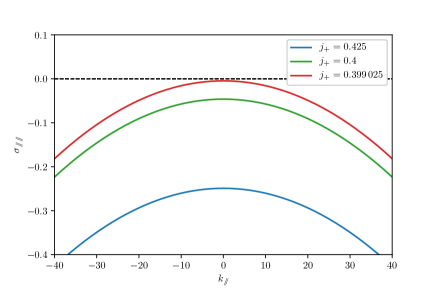
Methods Fig. S2: Growth rate for the longitudinal perturbations near the swap transition. We have used $j_{AA}=j_{BB}=$1$$, $\rho_{A}=\rho_{B}=1$, $j_{-}=$0.75$$, $\eta=$0.5$$, $v_{0}^{A}=$0.01$$ and $v_{0}^{A}=$0.03$$. Here $j_{+}^{\text{swap}}\approx$0.399$$ is the flocking-to-swap phase transition point.

In the case where the inter-species coupling has the same sign $j^{AB}j^{BA}>0$ (which includes the reciprocal case $j^{AB}=j^{BA}$), $\eta_{\sslash}$ is always positive and thus stable. This is seen as follows. When $j^{AB},j^{BA}>0(<0)$, the system is in a (anti)flocking phase at low enough noise strength, giving $P^{A}_{0}P^{B}_{0}>0(<0)$. Then, from Eqs. (S201) and (S202), we get $W^{AA}_{0},W^{BB}_{0}>0$. Similarly, from the definition of ${Q}^{a}_{0}$ given by Eq. (S197), $P_{0}^{A(B)}$ and ${Q}^{A(B)}_{0}$ have the same signs irrespective of the sign of the inter-species coupling $j^{AB},j^{BA}$, i.e. $P_{0}^{a}{Q}^{a}_{0}>0$. Since all the terms contributing to $\eta_{\sslash}$ in Eq. (S241) is thus positive as long as $j^{AB}$ and $j^{BA}$ has the same sign, the parameter $\eta_{\sslash}$ is positive and thus stable ($\sigma_{\sslash\sslash}<0$).

This restriction is lifted in the strong non-reciprocal case where the inter-species interaction have opposite signs $j^{AB}j^{BA}<0$. In particular, $W^{AA}_{0},W^{BB}_{0},P_{0}^{a}{Q}^{a}_{0}$ may all become negative. Thus, as the non-reciprocal interaction increases, $\eta_{\sslash}$ gets smaller and smaller until it approaches zero, or equivalently, $\sigma_{\sslash\sslash}=0$. Such softening of the longitudinal mode implies a phase transition to a swap phase.

This scenario is confirmed in Fig. S2, which shows the growth rate $\sigma_{\sslash\sslash}$ of the collective mode in this channel, in the vicinity of the phase transition point to the swap phase. As expected, the negative growth rate $\sigma_{\sslash\sslash}$ in the flocking phase softens (i.e. $\sigma_{\sslash\sslash}={\rm Re}s_{+}(\bm{k}=0)$ approaches zero) at the flocking-to-swap phase transition point ($j_{+}=j_{+}^{\text{swap}}$).

III.2.4 Tetracritical point

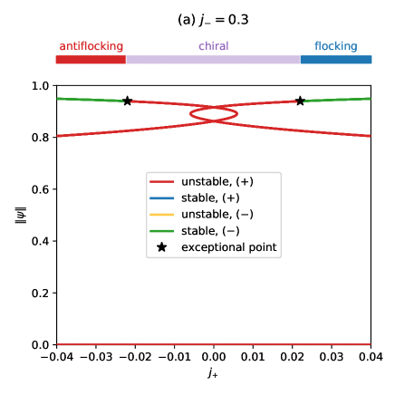
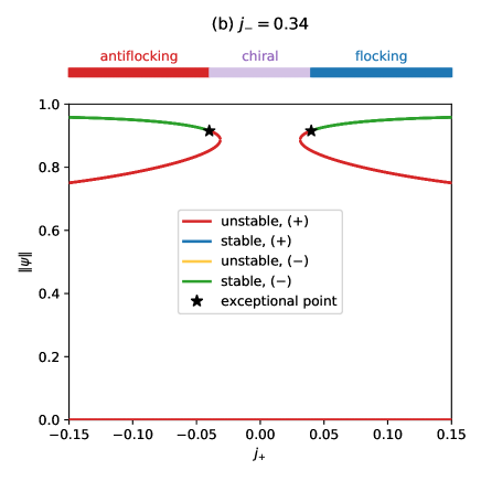
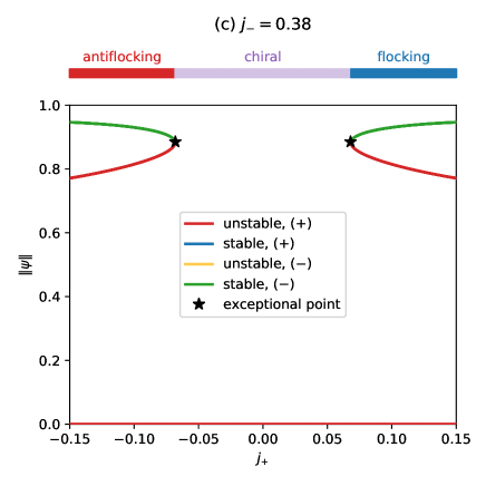
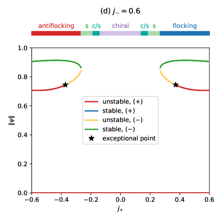
Methods Fig. S3: Bifurcation diagrams. Unless otherwise specified, the parameters are the same as in Fig. 2c of the main text. An exceptional point (marked by a black star) separates the branches labelled $(+)$ and $(-)$. The tetracritical points are found in the panel c and Fig. 2c in the main text at $(j_{-}^{*},j_{+}^{*})\approx(\pm 0.38,\pm 0.07)$. Note that the x-axis scales are different in the four panels.

Here we argue that, from the properties shown above, a tetracritical point, which is the point where the four phases (i.e. the (anti)flocking, chiral, swap, and the chiral-swap phase) meet at a single point, naturally emerges at least within the mean-field approximation. This is demonstrated in Fig. 2c in the main text, where the tetracritical points are marked by black dots.

The properties that we have shown so far can be summarized as follows:

1. In the (anti)flocking phase, there exists two types of solutions, namely, the "$-$" and "$+$" solutions, but the "$+$" solution is always unstable. On the other hand, as long as the system is away from the exceptional point $\Lambda_{0}>0$, the "$-$" solution is always stable against the global ($\bm{k}=0$) transverse channel fluctuations.

2. Approaching the exceptional point $\Lambda_{0}=0$ (which is the point where the "$-$" and the "$+$" solution coalesces), however, the (anti)flocking phase destabilizes in the transverse channel, signaling the phase transition to the chiral phase.

3. Independently from the above mechanism, "$-$" solution can also destabilize in the global longitudinal channel fluctuations, implying the phase transition into the swap phase.

4. In the parameter region between the chiral and swap phase, a mixed chiral-swap time quasicrystal phase emerges.

The properties 1 and 2 show that the (anti)flocking-to-chiral phase transition always occurs at the many-body exceptional point. As an example of such a situation, in Figs. S3a and b, we have plotted the amplitude of the polarization $\big{\lVert}\psi\big{\rVert}$ (where $\psi=(\vec{P}^{A{\mathsf{T}}}_{0},\vec{P}^{B{\mathsf{T}}}_{0})^{\mathsf{T}}$) for both the stable and unstable solutions in the (anti)flocking phase with $j_{-}<j_{-}^{*}$. As seen in the figure, the stable "$-$" solution and the unstable "$+$" solution coalesce at the exceptional point, which marks the phase transition point from the (anti)flocking phase to the chiral phase.

On the other hand, property 3 shows that there are cases where the "$-$" solution of the (anti)flocking phase exhibits phase transition to the swap phase. The property that this phase transition is associated with the destabilization of the longitudinal channel implies that the "susceptibility" of the amplitude of the polarization (i.e. the sensitivity of the amplitude of the polarization against a parameter change) diverges. This is indeed seen in the region $j_{-}>j_{-}^{*}$ in Fig. S3d at the (anti)flocking-to-swap phase transition point, where the derivative of the amplitude $\big{\lVert}\psi\big{\rVert}$ in the stable branch of the "$-$" solution diverges, i.e. $\left|\,\partial\big{\lVert}\psi\big{\rVert}/\partial j_{+}\,\right|\rightarrow\infty$ at the transition point. In this case, the exceptional point sits in the unstable branch of solutions.

At $j_{-}=j_{-}^{*}$, these two types of transition points (i.e. the exceptional point and the diverging susceptibility point) merges at $j_{+}=j_{+}^{*}$ as shown in Fig. S3c. Since these are the signals of the transition to the chiral and swap phase, respectively, and keeping in mind that the chiral/swap time quasicrystal phase occurs in the region between the chiral and the swap phase (property 4), the point $(j_{-}^{*},j_{+}^{*})$ is nothing but the tetracritical point.

III.2.5 Exceptional point enforced pattern formation

The chiral and swap phases appear in mean-field theory as spatially uniform instabilities of the (anti)flocking phases. Now we show that the flocking and antiflocking phases generically exhibit a finite wavelength instability in the transverse fluctuation channel in the vicinity of the exceptional point (except in highly fine-tuned situations), implying the occurrence of pattern formation. This originates from the singular behavior of the mean-field operator at this point combined with the presence of convective terms. At the exceptional point $\Lambda_{0}=0$ of the matrix $\hat{W}_{0}$,

$$0=\Gamma_{-}=\Gamma_{+}=\frac{1}{2}(W_{0}^{AA}+W_{0}^{BB}),$$ (S245)

and hence, $W^{AA}_{0}=-W^{BB}_{0}(\equiv W_{0})$. As a consequence, the block $\hat{L}_{\perp\perp}(\bm{k})$ corresponding to transverse fluctuations in Eq. (S196) reduces to

$$\hat{L}_{\perp\perp}(\bm{k}) = -i\left(\begin{array}[]{cc}W_{0}&-W_{0}\\ W_{0}&-W_{0}\end{array}\right)-i\hat{\lambda}^{\perp\perp}k_{\sslash}-\left(\begin{array}[]{cc}D_{0}^{A}&0\\ 0&D_{0}^{B}\end{array}\right)\bm{k}^{2}.$$ (S250)

The matrix $\hat{L}_{\perp\perp}(\bm{k})$ has an exceptional point at $\bm{k}=0$, where the two collective modes given by Eqs. (S214) and (S224)) coalesce Hanai and Littlewood (2020). Below, we restrict ourselves to $k_{\perp}=0$, where the transverse fluctuations decouple from the longitudinal mode such that the eigenvalues of $\hat{L}_{\perp\perp}(\bm{k}=k_{\sslash}\vec{e}_{\sslash})$ describe the collective modes of the system in this channel (i.e. $\hat{L}_{\perp\sslash}(\bm{k}=k_{\sslash}\vec{e}_{\sslash})=\hat{L}_{\sslash\perp}(\bm{k}=k_{\sslash}\vec{e}_{\sslash})=0$). The complex growth rates ($s=\sigma+i\omega$ including the frequencies $\omega$ as imaginary parts) of the collective modes are

$$s_{\pm}^{\perp\perp}(k_{\sslash}\vec{e}_{\sslash})=\pm i\sqrt{iC_{0}k_{\sslash}+O(k_{\sslash}^{2})}-i\lambda_{0}^{\perp\perp}k_{\sslash}-D_{0}k_{\sslash}^{2}.$$ (S251)

Here,

$$C_{0}=-2W_{0}(\lambda_{2}^{\perp\perp}+\lambda_{3}^{\perp\perp})\qquad\text{and}\qquad D_{0}=\frac{D_{0}^{A}+D_{0}^{B}}{2},$$ (S252)

where $\hat{\lambda}^{\perp\perp}$ is parameterized as

$$\hat{\lambda}^{\perp\perp}=\lambda_{0}^{\perp\perp}\hat{\sigma}_{0}+\lambda_{1}^{\perp\perp}\hat{\sigma}_{1}+i\lambda_{2}^{\perp\perp}\hat{\sigma}_{2}+\lambda_{3}^{\perp\perp}\hat{\sigma}_{3},$$ (S253)

where $\hat{\sigma}_{\alpha}$ ($\alpha=0,1,2,3$) are the Pauli matrices, and $\lambda^{\perp\perp}_{\alpha}$ are real numbers since $\hat{\lambda}^{\perp\perp}$ is a real matrix.

The leading order contribution in respect to $k_{\sslash}$ has a singular form $s_{\pm}^{\perp\perp}\sim\pm i\sqrt{iC_{0}k_{\sslash}}$ as long as $C_{0}\neq 0$. As a result, since the quantity inside the square root is purely imaginary, at least one of the two modes is inevitably unstable, irrespective of the sign of $C_{0}$. This shows that in the vicinity of a phase transition point from a (anti)flocking to the chiral phase, the uniform state is always destabilized by transverse fluctuations.

This originates from the exceptional point physics in the presence of convective terms. Typically, the eigenvalues in the vicinity of the exceptional point behave as $s_{\pm}\sim\pm i\sqrt{\Delta}$, where $\Delta$ is a characteristic distance from the exceptional point. In our situation, recalling that $\hat{L}_{\perp\perp}(\bm{k}={\bf 0})$ is at an exceptional point, the finite momentum $\bm{k}$ contribution to $\hat{L}_{\perp\perp}(k_{\sslash}\vec{e}_{\sslash})$ can be regarded as the contributions that makes $\hat{L}_{\perp\perp}(k_{\sslash}\vec{e}_{\sslash})$ deviate from that point. Because of the presence of the convective term $\hat{\lambda}^{\perp\perp}k_{\sslash}$, the leading order is $O(k_{\sslash})$. As a result, $\Delta\sim ik_{\sslash}$, leading to $s_{\pm}\sim\pm i\sqrt{ik_{\sslash}}$, so at least one of the complex growth rates has a positive real part, implying an instability leading to pattern formation. The uniform flocking phase may be stabilized by moving away from the exceptional point.

III.3 Floquet stability analysis of the chiral phase

Here we provide a stability analysis on the chiral phase. As the mean-field solution in this phase depends on time, the method used to analyze the stability of the (anti)flocking phases cannot be directly applied. Instead, we take advantage of the periodicity in time of the mean-field solution $\vec{P}^{a}(t)$ given by Eq. (S110) we perform a Floquet stability analysis of the phase Floquet (1883); Lyapunov (1907); Teschl (2012) (see also Ref. Barkey and Henderson (1996) for an example in the context of fluid mechanics). We note that the transformation to the rotating frame does not completely eliminate the time dependence, due to the presence of convective terms.

The mean-field solution in the chiral phase ($\vec{P}^{a}(t)$ in Eq. (S110)) is $T$-periodic in time with a period $T=2\pi/\Omega$, where $\Omega$ is given by Eq. (S122). Specializing the relevant part of Eq. (S179) to this case, we obtain

$$\partial_{t}\delta\vec{P}(t,\bm{k})=L(t,\bm{k})\delta\vec{P}(t,\bm{k})$$ (S254)

where crucially $L(t,\bm{k})$ is $T$-periodic, namely $L(t+T,\bm{k})=L(t,\bm{k})$. This equation is formally solved by the evolution operator $U(t)$ such $\delta\vec{P}(t,\bm{k})=U(t)\delta\vec{P}(0,\bm{k})$ is a solution of (S254) for any initial condition $\delta\vec{P}(0,\bm{k})$ (in the context of ODEs, the evolution operator is called the principal fundamental matrix solution of the differential equation). This evolution operator is the time-ordered exponential

$$U(t,\bm{k})=T\exp\left(\int_{0}^{t}L(\bm{k},s)\text{d}s\right)$$ (S255)

which can also be written as the infinite series

$$U(t,\bm{k})=\lim_{\delta t/t\to 0}\prod_{n=1}^{\lfloor t/\delta t\rfloor}\exp\left(n\delta t\,L(\bm{k},n\delta t)\right).$$ (S256)

Assuming the periodicity of $L(t)=L(t+T)$, the Floquet theorem Floquet (1883); Teschl (2012) implies that the evolution operator satisfies (pointwise in $\bm{k}$)

$$U(t+nT)=U(t)[U(T)]^{n}$$ (S257)

The evolution operator evaluated after one period $U(T)$ is called the Floquet operator (also known as the monodromy matrix). It is convenient to write it as $U(T)=\text{e}^{TL^{\text{eff}}}$ (where $L^{\text{eff}}$ is defined up to a choice of branch cut for the logarithm). The property (S257) allows to decompose the evolution operator as $U(t)=V(t)\text{e}^{tL^{\text{eff}}}$ where $V(t)=V(t+T)$ is periodic in time. This decomposition shows that crucially, the long-time behavior of the solutions of Eq. (S254), and in particular their stability, is fully controlled by the Floquet operator $U(T)$.

Indeed, any solution of (S254) can be decomposed into fundamental solutions $\delta\vec{P}_{\alpha}(\bm{k},t)$, which are obtained from the eigenvalues $\lambda_{\alpha}(\bm{k})$ and eigenvectors $\delta\vec{P}^{0}_{\alpha}(\bm{k})$ of $U(T,\bm{k})$ as

$$\delta\vec{P}_{\alpha}(\bm{k},t)=(\lambda_{\alpha})^{t}\,\vec{p}_{\alpha}(t,\bm{k})$$ (S258)

where $\vec{p}_{\alpha}(t,\bm{k})=V(t)\delta\vec{P}^{0}_{\alpha}(\bm{k})=p_{\alpha}(t+T,\bm{k})$ is periodic in time. The eigenvalues $\lambda_{\alpha}(\bm{k})$ of $U(T,\bm{k})$ are called Floquet multipliers (or characteristic multipliers), and they can be written as $\lambda_{\alpha}(\bm{k})=\text{e}^{s_{\alpha}({\bm{k}})}$ where $s_{\alpha}({\bm{k}})$ is called a Floquet exponent (the Floquet exponents are also the eigenvalues of $L^{\text{eff}}$, and they are only defined up to a phase). The Floquet exponent $s_{\alpha}({\bm{k}})=\sigma_{\alpha}({\bm{k}})+\text{i}\omega_{\alpha}({\bm{k}})$ can be decomposed into real and imaginary parts, which correspond to the growth rate $\sigma_{\alpha}({\bm{k}})$ of the corresponding fundamental solution and its oscillation quasi-frequency $\omega_{\alpha}({\bm{k}})$ (only defined up to multiples of $2\pi/T)$. A positive (negative) growth rate corresponds to an unstable (stable) solution. Equivalently, the solution is stable when the absolute value of the Floquet multiplier $|\lambda_{\alpha}|$ is smaller than unity.

To determine the stability of the chiral phase, we first solve numerically the mean-field dynamical system in Eq. (S64) to obtain the time-independent quantities $R_{a}=\lVert\vec{P}_{a}\rVert$ ($a=A,B$) and $\Delta\phi^{AB}=\text{angle}(\vec{P}_{A},\vec{P}_{B})$. We obtain the time-dependent mean-field solution $\vec{P}_{a,\text{ss}}(t)$ as well as its period $T$ using Eqs. (S110) and (S122). This allows us to compute the time-dependent matrix $L(t)$ from Eq. (S181), where $\vec{P}_{a}$ is replaced by $\vec{P}_{a,\text{ss}}(t)$. We then use a discretized version of Eq. (S256) (where $\delta t$ is finite) to compute $U(T,\bm{k})$, which is diagonalized to determine the Floquet multipliers $\lambda_{\alpha}(\bm{k})$. A direct inspection of the spectra shows that as in the time-independent case, we always have $|\lambda_{\alpha}({\bm{0}})|\leq 1$ in the chiral phase (because it is the mean-field solution), with one marginal eigenvalue pinned at $|\lambda|=1$. We focus on the multiplier $\lambda({\bm{0}})$ with maximal absolute value, for which $|\lambda({\bm{0}})|=1$. We use the same procedure as for the (anti)flocking phases to estimate the stability of the phase from the sign of the eigenvalues of the Hessian matrix of the function $\bm{k}\mapsto|\lambda(\bm{k})|$ at $\bm{k}={\bm{0}}$, and the same caveat applies. By carrying out this procedure, we find wide regions in parameter space where the chiral phase is stable, as shown in Fig. 3a of the main text.

IV Non-reciprocity and broken detailed balance

In this section, we show that the non-reciprocity in Eq. (2) of the main text ($J_{mn}\neq J_{nm}$) implies the breaking of detailed balance in the corresponding Markov process. The broken detailed balance (and hence, the lack of microscopic reversibility) implies that the system is out-of-equilibrium, allowing the appearance of oscillating states Kondepudi and Prigogine (2014); Zhabotinsky (2007); Lan et al. (2012); Cao et al. (2015); Barato and Seifert (2015); del Junco and Vaikuntanathan (2020), see also Refs. Yan et al. (2013); Wang and Ruuth (2008).

We consider a set of coupled Langevin equations

$$\partial_{t}X_{m}(t)=F_{m}(X)+\sigma_{mn}\eta_{n}(t)$$ (S259)

where $X_{n}$ are a set of random variables for $n=1,\dots,N$, and $\eta_{n}(t)$ are white noises with unit standard deviation. This general form encompasses Eq. (2) of the main text. (It can also describe the coarse-grained Eq. (1) of the main text, provided that a noise is added to the right-hand side.) The evolution of the probability distribution $p(t,x)$ of the random variables $X=(X_{1},\dots,X_{N})$ ruled by Eq. (S259) is described by the Fokker-Planck equation van Kampen (2007); Risken (1989)

$$\partial_{t}p=\hat{\mathbb{W}}p$$ (S260)

where the operator $\hat{\mathbb{W}}$ is defined by

$$\hat{\mathbb{W}}p=-\partial_{m}[F_{m}(x)p(t,x)]+D_{mn}\partial_{m}\partial_{n}p(t,x)$$ (S261)

for an arbitrary distribution $p$, where $\partial_{m}=\partial/\partial x_{m}$ and $D=\sigma\sigma^{T}/2$. In the following, we shall assume that the diffusion tensor $D_{mn}=D_{m}\delta_{mn}$ is diagonal (as $D$ is real and symmetric, this can always be achieved through an appropriate change of variable $x_{m}\to J_{mm^{\prime}}x_{m^{\prime}}$).

Assume that the process defined by $\hat{\mathbb{W}}$ has a stationary distribution $p_{\text{s}}(x)$ (such that $\hat{\mathbb{W}}p_{\text{s}}=0$). We define a weighted scalar product on distributions by

$$\braket{f,g}_{\text{s}}=\int\frac{1}{p_{\text{s}}(x)}\,f(x)g(x)\text{d}x.$$ (S262)

The operator $\hat{\mathbb{W}}$ satisfies detailed balance (for $p_{\text{s}}$) if it is self-adjoint with respect to this scalar product van Kampen (2007), namely if for any distributions $f$ and $g$,

$$\braket{f,\hat{\mathbb{W}}g}_{\text{s}}=\braket{\hat{\mathbb{W}}f,g}_{\text{s}}.$$ (S263)

A few tedious but straightforward manipulations show that for the Langevin Eq. (S259), the detailed balance condition Eq. (S263) is equivalent to Lan et al. (2012)

$$F_{m}=D_{m}\frac{\partial_{m}p_{\text{s}}}{p_{\text{s}}}$$ (S264)

for all $m=1,\dots,N$. This equation implies (but is not necessarily equivalent to)

$$\frac{\partial_{n}F_{m}}{D_{m}}=\frac{p_{\text{s}}(\partial_{m}\partial_{n}p_{\text{s}})-(\partial_{m}p_{\text{s}})(\partial_{n}p_{\text{s}})}{p_{\text{s}}^{2}}$$ (S265)

which in turn implies that for all $m,n$, one has Lan et al. (2012)

$$D_{n}\partial_{n}F_{m}=D_{m}\partial_{m}F_{n}.$$ (S266)

For the system considered in the main text, Eq. (2), we have $D_{m}=D_{n}=\eta^{2}/2$ for all $m,n$ and

$$F_{m}(\theta)=\sum_{n}J_{mn}\sin(\theta_{n}-\theta_{m}).$$ (S267)

Hence (for $n\neq m$),

$$\partial_{n}F_{m}(\theta)=J_{mn}\cos(\theta_{n}-\theta_{m})$$ (S268)

and by permuting the indices,

$$\partial_{m}F_{n}(\theta)=J_{nm}\cos(\theta_{m}-\theta_{n})=J_{nm}\cos(\theta_{n}-\theta_{m})$$ (S269)

We conclude that $J_{mn}\neq J_{nm}$ implies that detailed balance is broken (in the situation when the noises can have different strengths, this condition would read $D_{n}J_{mn}\neq D_{m}J_{nm}$).

V Nonexistence of the chiral phase with two partially non-reciprocal agents

In this section, we analyze the evolution of two and only two non-reciprocal agents $A$ and $B$, that represent either two oscillators in the Kuramoto model (without a natural frequency), or two self-propelled agents in the Vicsek model. We show analytically that stable chiral motion is only possible when the interactions are fully non-reciprocal: any amount of reciprocal interaction eventually leads to alignment, and the chiral behavior is a transient.

We assume that the agents always close enough to interact, and neglect the effect of noise. The evolution of their angles $\theta_{A}$ and $\theta_{B}$ is then described by the equations

$$\partial_{t}\theta_{A} =J_{AB}\sin(\theta_{B}-\theta_{A})$$ (S270a)

$$\partial_{t}\theta_{B} =J_{BA}\sin(\theta_{A}-\theta_{B}).$$ (S270b)

It is convenient to define

$$\bar{\theta}=\theta_{A}+\theta_{B}\quad\Delta\theta=\theta_{A}-\theta_{B}\quad J_{\pm}=J_{AB}\pm J_{BA}$$ (S271)

in terms of which the dynamical system in Eq. (S270) becomes

$$\partial_{t}\bar{\theta} =-J_{-}\sin(\Delta\theta)$$ (S272a)

$$\partial_{t}\Delta\theta =-J_{+}\sin(\Delta\theta).$$ (S272b)

The coefficient $J_{+}$ represents the reciprocal part of the interactions, while $J_{-}$ represents the non-reciprocal part. When the reciprocal interactions vanish, $J_{+}=0$, then $\Delta\theta(t)=\Delta\theta(0)$ is a constant (equal to its initial value), and the average angle $\bar{\theta}(t)$ increases linearly. This corresponds to a circular motion at a frequency $1/[J_{-}\sin(\Delta\theta(0))]$, whose characteristics are highly sensitive to the initial conditions. In an exactly anti-reciprocal system (and in the absence of noise), this circular motion goes on forever. However, in this very simple model, any amount of reciprocal interaction $J_{+}\neq 0$ leads to the eventual suppression of the circular motion, on a time scale of order $1/J_{+}$. Indeed, when the reciprocal part of the interaction $J_{+}$ is nonzero, $\Delta\theta$ relaxes to either $0$ or $\pi$ depending on the sign of $J_{+}$ (the solution flows from the unstable fixed point to the stable one). When $J_{+}$ vanishes, the situation is marginal and $\Delta\theta$ remains constant.

We now solve the system (S272) explicitly. In terms of $y=\tan(\Delta\theta/2)$, for which $y^{\prime}(t)=-J_{+}y(t)$, Eq. (S272b) describes an exponential relaxation on a time scale $1/J_{+}$, namely

$$\tan\left(\frac{\Delta\theta(t)}{2}\right)=\tan\left(\frac{\Delta\theta(0)}{2}\right)\,\exp\left(-J_{+}\,t\right).$$ (S273)

The evolution of the average angle $\bar{\theta}(t)$ is slaved to the evolution of $\Delta\theta$, as

$$\bar{\theta}(t)=\bar{\theta}(0)-J_{-}\int_{0}^{t}\sin(\Delta\theta(t^{\prime}))\text{d}t^{\prime}.$$ (S274)

As a consequence, $\bar{\theta}(t)$ becomes approximately constant when $\Delta\theta(t)$ approaches $0$ or $\pi$. More precisely, we find

$$\bar{\theta}(t)=\bar{\theta}(0)-2\frac{J_{-}}{J_{+}}\big{[}\operatorname{arccot}\left(y_{0}\,\text{e}^{-t\,J_{+}}\right)-\operatorname{arccot}\left(y_{0}\right)\big{]}$$ (S275)

where $y_{0}=\tan\left(\Delta\theta(0)/2\right)$. This expression exhibits an indeterminate form as $J_{+}\to 0$, that can however be resolved and yields a linear behavior in time consistent with the previous discussion,

$$\bar{\theta}(t)=\bar{\theta}(0)-2J_{-}\,\frac{y_{0}\,t}{1+y_{0}^{2}}=\bar{\theta}(0)-J_{-}\sin[\Delta\theta(0)]t.$$ (S276)

VI Non-reciprocal Kuramoto model

In this section, we consider a non-reciprocal version of the Kuramoto model Ott and Antonsen (2008, 2009); Watanabe and Strogatz (1993, 1994); Marvel et al. (2009); Pikovsky and Rosenblum (2011, 2008); Hong and Strogatz (2011a, b, 2012); Tyulkina et al. (2018); Montbrió et al. (2015) with two communities ($a=A,B$). We first give numerical evidence that the Ott-Antonsen type mean-field analysis Ott and Antonsen (2008, 2009); Watanabe and Strogatz (1993, 1994); Marvel et al. (2009); Pikovsky and Rosenblum (2011, 2008); Hong and Strogatz (2011a, b, 2012); Tyulkina et al. (2018); Montbrió et al. (2015) used in the Methods is consistent with direct simulations of the microscopic model Eq. (S277). We then show analytically that the time-dependent phases are absent when all oscillators have identical natural frequencies (pictorially, $\Delta_{a}=0$) and there is no random noise. Perhaps counter-intuitively, noise/disorder is necessary for the occurrence of such time-dependent ordered phases (Sec. VI.2). We further argue that the interplay between noise/disorder (that continuously resets the evolution, thereby promoting the chase-and-runaway behavior) and the many-body interactions (that makes the state “rigid”) is responsible for the emergence of time-dependent ordered phases. We support this claim by computing the standard deviations of the order parameter (Sec. VI.3).

The emergence of the time-dependent phases (such as the chiral phase) as a consequence of the interplay between disorder/noise and many-body interactions is strikingly similar to the phenomenon of order-by-disorder that often arises in frustrated many-body systems Villain et al. (1980); Henley (1989); Ionita et al. (2013). There, the presence of thermal noise or disorder stabilizes an ordered phase even when the ground state is degenerate. This analogy implies a surprising connection between geometric frustration and the dynamical frustration due to non-reciprocal interactions that may only arise in non-equilibrium systems.

We consider the Kuramoto model Kuramoto (1984); Shinomoto and Kuramoto (1986); Sakaguchi et al. (1988); Acebrón et al. (2005)

$$\partial_{t}\theta_{m}^{a}=\omega_{m}^{a}+\sum_{b=A,B}\sum_{n=1}^{N_{b}}J_{ab}\sin(\theta_{n}^{b}-\theta_{m}^{a})+\eta_{a}(t),$$ (S277)

where $\theta_{m}^{a}$ and $\omega_{m}^{a}$ are the phase and natural frequency of the $m$-th oscillator in the community $a$, $N_{a}$ is the number of $a$-species oscillators, $\eta_{a}(t)$ is a white noise acting on species $a$, and $J_{ab}$ is the coupling strength between the oscillators in the communities $a$ and $b$. The inter-community interaction can be non-reciprocal by allowing $J_{AB}\neq J_{BA}$. We assume that all-to-all connections between the oscillators. Unless otherwise specified, we assume that the natural frequencies of species $a$ follow the Lorentzian distribution,

$$g_{a}(\omega)=\frac{1}{\pi}\frac{\Delta_{a}}{(\omega-\omega_{a})^{2}+\Delta_{a}^{2}}.$$ (S278)

(We will also consider the case where all the frequencies are equal.) We are mainly interested in the behavior of the order parameters that characterizes the synchronization is given by,

$$z_{a}(t)\equiv r_{a}(t)\text{e}^{\text{i}\phi_{a}(t)}=\frac{1}{N_{a}}\sum_{m=1}^{N_{a}}\text{e}^{\text{i}\theta_{m}^{a}(t)},$$ (S279)

which becomes finite when synchronization occurs. In the following, we restrict our attention to the $O(2)$ symmetric situation where $\omega_{A}=\omega_{B}=0$ (it is crucial that the detuning $\omega_{A}-\omega_{B}$ is set to zero, but we can restore a common oscillation frequency $\omega_{A}=\omega_{B}$ by a change of reference frame). The $SO(2)$ symmetric case where a detuning can exist (and in which PT-symmetry is explicitly broken) is discussed in the Methods.

VI.1 Time-dependent phases in the PT-symmetric Kuramoto model

Here, we compare the dynamics of the non-reciprocal Kuramoto model (without noise) with the mean-field dynamical system

$$\partial_{t}z_{a}=(\text{i}\omega_{a}-\Delta_{a})z_{a}+\frac{1}{2}\sum_{b}j_{ab}\left[z_{b}-z_{a}^{2}\,\overline{z_{b}}\right]$$ (S280)

describing the evolution of the complex order parameter $z_{a}(t)$ of each community $a$, and where $\overline{z_{b}}$ is the complex conjugate of $z_{b}$. In the limit where $N_{a}\to\infty$, this mean-field reduction should be exact, see Refs. Ott and Antonsen (2008, 2009); Watanabe and Strogatz (1993, 1994); Marvel et al. (2009); Pikovsky and Rosenblum (2011, 2008); Hong and Strogatz (2011a, b, 2012); Tyulkina et al. (2018); Montbrió et al. (2015); Bick et al. (2020).

The results of the comparison are presented in Fig. S4, and show a good agreement between the microscopic simulations and the mean-field description.

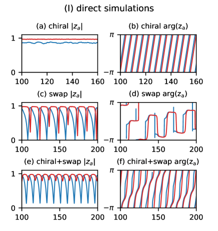
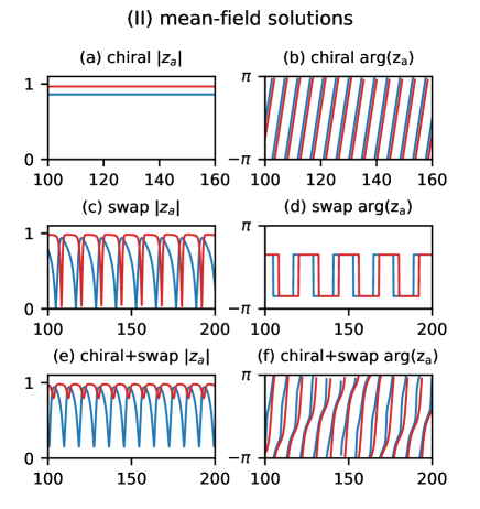
Methods Fig. S4: Comparison of direct simulations of the Kuramoto model with mean-field solutions. (A) Simulation of $N=$4000$$ particles (separated in two species) with Lorentzian frequency distributions with parameters $\omega_{A}=\omega_{B}=$0$$ $\Delta_{A}=\Delta_{B}=$0.05$$, without noise. We have set $j_{AA}=j_{BB}=$1.0$$ and $j_{-}=$1.6$$, as well as (a) chiral $j_{+}=$0.1$$ (b) swap $j_{+}=$0.7$$ (c) chiral+swap $j_{+}=$0.4$$. The total duration is $T_{\text{sim}}=$200$$ with (a,c) $\delta t=$0.05$$ and (b) $\delta t=$0.025$$. (B) Solutions of the corresponding mean-field dynamical systems. The agreement is very good. The most striking difference between (A) and (B) is the existence of a slow drift in the swap phase in the direct simulations (not present in the mean-field analysis), that we attribute to finite-size effects.

VI.2 Lack of time-dependent phases without disorder or noise

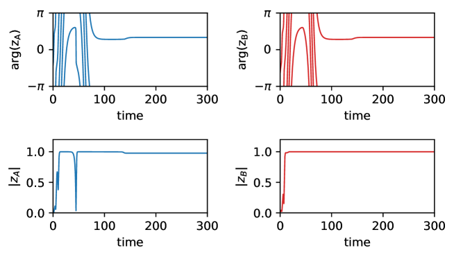
Methods Fig. S5: Eventual alignment in the absence of noise and/or frequency spread. We compute the standard deviations of the order parameter in the chiral phase (the norms of $\vec{P}_{A}$ and $\vec{P}_{B}$, and their relative angle $\Delta\phi$) obtained by simulations of the microscopic model Eq. (S1). We used the same parameters as in Fig. S4a, with the exception of the frequency distribution: here all the natural frequencies are equal to $\omega_{A}=\omega_{B}=$0$$. In contrast with what Fig. S4a, we observe here that the oscillators all eventually align. We have used $\delta t=$0.01$$.

In this section, we show that when all the oscillators have identical natural frequencies and there is no noise, the dynamics of two communities of oscillators can be mapped to the dynamics of two oscillators. As a consequence, the time-dependent phases (such as the chiral (travelling wave) and swap (periodic synchronization) phases) of the PT-symmetric Kuramoto model are absent in this case. This explicitly shows that these time-dependent phases are driven by noise/disorder.

We note that this result hinges on the infinite-ranged coupling between the oscillators, and might not hold true with finite-ranged couplings. For instance, Eq. (S171) in the non-reciprocal Vicsek model suggests the possibility of a chiral phase at zero disorder $\eta=0$ for $|j_{-}|>|j|$ (although other instabilities not taken into account by this equation might also take place). Yet, we expect the range of parameters in which the chiral is stable to be enlarged by the noise even in this case (compare Fig. 2b and Fig. 2c in the main text).

In the absence of noise ($\eta_{a}=0$), the steady-state with frequency $\Omega$ has an order parameter of the form

$$z_{a}(t)=z_{a}\text{e}^{\text{i}\Omega t}\quad\text{with}\quad z_{a}=r_{a}\text{e}^{\phi_{a}^{0}},$$ (S281)

that satisfies the self-consistency condition (derived in the Methods; note that here we start directly from the Kuramoto model Eq. (S277), not from the Ott-Antonsen mean field description)

$$z_{a}=R_{a}e^{i\alpha_{a}}F_{a}[z_{a},z_{b}]$$ (S282)

where

$$R_{a}\text{e}^{\text{i}\alpha_{a}} =\sum_{b}j_{ab}z_{b},$$ (S283a)

$$F_{a}[z_{A},z_{B}] =\int_{-\pi/2}^{\pi/2}\text{d}\theta\cos\theta\,\text{e}^{\text{i}\theta}g_{a}(R_{a}\sin\theta+\Omega)+\int_{-\pi}^{\pi}\text{d}\theta\int_{|x|>1}\text{d}x\,\text{e}^{\text{i}\theta}g_{a}(R_{a}x+\Omega)\frac{\sqrt{x^{2}-1}}{|x-\sin\theta|},$$ (S283b)

and $j_{ab}=J_{ab}N_{b}$. The first and the second term of Eq. (S283b) are contributions from synchronized and unsynchronized oscillators, respectively.

In the limit where the width of the distribution of natural frequencies vanish $\Delta_{a}\rightarrow 0^{+}$ (so all oscillators have the same natural frequency), we get

$$F_{a}=\frac{e^{\text{i}\zeta_{a}}}{R_{a}}\qquad\text{with}\qquad\zeta_{a}=-\sin\Big{(}\frac{\Omega}{R_{a}}\Big{)},$$ (S284)

as long as the synchronization frequency is not very far away from resonance $|\Omega|<R_{a}$, where there are no contribution from the second term of Eq. (S283b).

Plugging Eq. (S284) into Eq. (S282) yields

$$z_{a}(t)=r_{a}e^{i\phi_{a}(t)}=e^{i(\alpha_{a}+\zeta_{a})}e^{i\Omega t},$$ (S285)

giving perfect synchronization $r_{a}=1$ and $\phi_{a}(t)=\alpha_{a}+\zeta_{a}+\Omega t$. The perfect synchronization $r_{a}=1$ implies that all the oscillators in the community $a$ satisfy $\theta_{m}^{a}(t)=\phi_{a}(t)$. It then follows (by substituting this in Eq. (S277)) that the dynamics (in the long time limit where the amplitude $r_{a}(t)$ has converged to unity) are described by

$$\partial_{t}\phi_{A} =j_{AB}\sin(\phi_{B}-\phi_{A}),$$ (S286)

$$\partial_{t}\phi_{B} =j_{BA}\sin(\phi_{A}-\phi_{B})$$ (S287)

which are identical to the dynamical equations Eq. (S270) for the case of two agents! This is because, in the absence of noise and disorder, all the oscillators perfectly synchronize within each population, so each group of oscillators simply behaves as a single (macroscopic) oscillator characterized solely by its phase $\phi_{a}$.

As we show in Sec. V, the state of the system in these phases eventually approaches a constant (i.e. $\Omega=0$) with $\phi_{A}-\phi_{B}=0(\pi)$ when $J_{AB}+J_{BA}>0(<0),$ corresponding to the static, coherent ($\pi$-state) phase. This explicitly shows that the time-dependent phases that cannot occur without noise or disorder.

These conclusions are numerically confirmed in Fig. S5 from direct numerical simulations of Eq. (S277) with $\eta_{a}=0$ and $\omega_{m}^{a}=0$. As expected from the arguments above, the phases of the two order parameters eventually align, even though the system would be deep in the chiral phase when a small width in the frequency distribution is introduced (compare with Fig. S4a where $\Delta_{A}=\Delta_{B}=0.05$). The magnitude of the order parameters $|z_{A}|$ and $|z_{B}|$ approaches one, which is also consistent with the discussions above. Hence, the existence of the time-dependent (chiral, swap, and chiral+swap) phases crucially hinges on a finite amount of disorder in the frequencies and/or on the presence of a random noise. The noise/disorder alone would however simply suppress any order without the rigidity provided by many-body interactions, see Fig. S6 in Sec. VI.3.

The exactly non-reciprocal case $J_{AB}=-J_{BA}$ is a singular point, where a finite synchronization frequency $\Omega=\pm(J_{AB}+J_{BA})$ is obtained in the long-time limit. However, even here, there is an important difference from the chiral phase: the relative phase $\phi_{A}-\phi_{B}$ can take an arbitrary value set by the initial condition, while in the chiral phase they are determined intrinsically. (See the detailed analysis in Sec. II.1 for the chiral phase in a non-reciprocal Vicsek model.)

The above analysis clearly shows that noise/disorder is a necessary element for the time-dependent phases to emerge in this system. This can be intuitively understood as follows: Let $J_{AB}>0$ and $J_{BA}<0$ with $J_{AB}>|J_{BA}|$. As discussed earlier, the predator group A oscillators would stop chasing the prey group B oscillators once they caught them (i.e. become aligned). (We emphasize that we are not describing a prey-predator model in the usual sense, and that the chase occurs on the circle in which the phases of the oscillators or angles of the self-propelled particles live, not in physical space.) However, noise can kick this state out of this optimal state for the A component, restarting the chase again. Since noise occurs continuously, this (randomized) chase-and-runaway motion will continue even in the long-time limit. This continuous resetting of the dynamics is reminiscent of the predator-prey population dynamics discussed in Ref. McKane and Newman (2005); Horsthemke and Lefever (1984); Gammaitoni et al. (1998).

VI.3 Convergence of the chiral phase

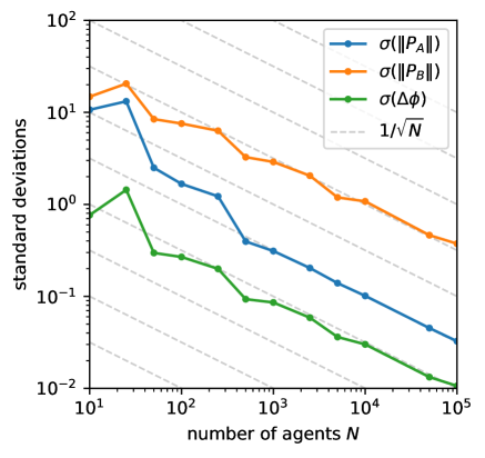
Methods Fig. S6: Standard deviations of the order parameters in the chiral phase. We compute the standard deviations of the order parameter in the chiral phase (the norms of $\vec{P}_{A}$ and $\vec{P}_{B}$, and their relative angle $\Delta\phi$) obtained by simulations of the microscopic model Eq. (S1). Here, there is a slight amount of reciprocal interaction between the two species. Without noise, the chiral phase does not exist as the populations eventually synchronize or antisynchronize. Noise restores the chiral behavior, at the price of fluctuations of the order parameter, but they decrease approximately as $1/\sqrt{N}$ with the number of agents $N$. The gray lines are equally spaced $1/\sqrt{N}$ curves and are meant as a guide to the eye (not a fit). In order to single out the influence of the number of agents from other, we set their velocities to zero and their interaction range to be infinite. We used $J_{AA}=J_{BB}=$1$$, $J_{AB}=$1$$, $J_{BA}=$-1.1$$, $\eta=$8\text{\times}{10}^{-2}$$. The total duration is $T_{\text{sim}}/\delta t=$4000$$ with $\delta t=$0.5$$, over which the standard deviation is computed.

The discussion in the previous subsection confirms that noise/disorder is necessary for the time-dependent phases to appear. However, there is an important caveat: the noise may simultaneously destroy the order. Here we argue that the many-body interaction effect plays an equally crucial role in the appearance of the time-dependent phases by making this phase rigid and stable against noise.

Our claim is supported in Fig. S6 for the chiral phase, where the evolution of the standard deviations of the order parameters with $N$ is obtained from simulations (where $N=N_{A}+N_{B}$ is the total number of agents). When the number of agents is still far from the thermodynamic limit ($N\lesssim 10$), the standard deviations are of $O(1)$ (or even larger) meaning that the fluctuations are larger than the order parameter itself, questioning the robustness of the order. However, as $N$ gets larger, the standard deviations decrease approximately as $1/\sqrt{N}$, signaling the stabilization of the chiral phase. A similar scaling is observed in the case of the standard Kuramoto model, see Ref. Acebrón et al. (2005).

VII Many-body stabilization of the chiral phase against changes of the chirality

We have seen in Sec. VI.2 that noise is crucial in the establishment of the chiral phase. In this paragraph, we show how noise can also destroy the chiral phase by randomly flipping the chirality over time. We also show that this process is exponentially suppressed when the number of agents increases.

This situation is very similar to Néel relaxation theory Néel (1950); Brown (1963) which describes the mean transition time between the two equilibrium states available to the magnetization of single-domain ferromagnetic nanoparticles.

The Kuramoto and Vicsek models without microscopic noise can be described by an accurate mean-field dynamical system, that (correctly) predicts the lack of a chiral phase in some circumstances. The microscopic noise leads to the apparition of the chiral phase by a mechanism of constant resetting of the dynamics. When only a few agents are present, the dynamics is effectively random and it is not clear that it can be correctly captured by a noisy mean-field equation of motion. When the number of agents increases, the effect of noise is reduced and we can expect to capture some aspects of the dynamics (such as the chirality flips) by a noisy dynamical system. As we shall see, the effect of the noise is exponentially reduced with the number of agents, leading to a deterministic dynamical system in the hydrodynamic limit.

The chiral phase spontaneously breaks parity: in a deterministic dynamical system (without noise), the resulting motion can either be clockwise or counterclockwise, depending on the initial conditions. In reality, some noise (thermal or not) is always present, and the mean-field dynamical system $\partial_{t}X=f(X)$ (e.g. Eq. (1) of the main text) becomes a stochastic dynamical system $\partial_{t}X=f(X)+\xi(t)$ in which $\xi(t)$ is a random noise. A large enough fluctuation can flip the system from clockwise to counterclockwise, as represented in Fig. S7. This leads to a statistical restoration of parity: the system undergoes a succession of clockwise and counterclockwise motions, that have an average lifetime $\tau$ (the time between two successive flips), which has to be compared with the duration of an experiment.

The chirality flips occur when the angle $\Delta\phi$ between the order parameters $\vec{v}_{A}$ and $\vec{v}_{B}$ changes sign (see Fig. S7, and e.g. Eqs. (S110)-(S112) in the case of flocking). Away from the phase transitions, we expect every mode to relax way faster than $\Delta\phi$ (except the global rotation of both $\vec{v}_{A}$ and $\vec{v}_{B}$, which can be ignored because of the symmetry). Hence, we focus only on $\Delta\phi$ and write a reduced dynamical system for $\Delta\phi$, such as

$$\partial_{t}\Delta\phi=h(\Delta\phi)+\xi(t)$$ (S288)

Intuitively, $\Delta\phi$ essentially evolves in a double-well potential, in which the two minima $\pm\Delta\phi_{\text{c}}$ correspond to the clockwise and counterclockwise chiral phases. The variable $\Delta\phi(t)$ fluctuates because of the noise, and can sometimes overcome the potential barrier to go from one minimum to another. (Despite this intuitive description in terms of a potential, we do not assume that the system is at equilibrium. We simply start from Eq. (S288).) This situation is known as the Kramers problem, and the characteristic time $\tau$ between two transitions follows an Arrhenius law of the form Zwanzig (2001); Hänggi et al. (1990)

$$\tau=\tau_{0}\exp\left(\frac{\Delta U}{\sigma_{\xi}^{2}}\right)$$ (S289)

in which $\sigma_{\xi}$ is the standard deviation of the Gaussian noise $\xi(t)$ with zero mean and with $\braket{\xi(t)\xi(0)}=2\sigma_{\xi}^{2}\delta(t)$, and $\Delta U$ is the effective barrier height defined as

$$\Delta U=-\int_{\pm\Delta\phi_{\text{c}}}^{0}h(\vartheta)\,\text{d}\vartheta.$$ (S290)

Here, we have ignored the additional complexity coming from the fact that $\Delta\phi$ is an angle, which does not qualitatively affect the argument.

In section VI.3, we have seen from numerical simulations that the fluctuations of the order parameter decrease as $1/\sqrt{N}$ when the number of agents $N$ increases (when $N$ is large). This can be understood as a consequence of the central limit theorem, according to which the average of $N$ independent and identically distributed variables with finite variances $\sigma^{2}$ converges to a normal distribution with variance $\sigma^{2}/N$. Accordingly, we assume that

$$\sigma_{\xi}=\frac{\sigma_{0}}{\sqrt{N}}$$ (S291)

in which $\sigma_{0}$ is a constant representing the standard deviation of the noise acting on a single agent (in a thermal system, we would have $\sigma_{0}^{2}\propto k_{\text{B}}T$). The quantities $\tau_{0}$ and $\Delta U$ are properties of the mean-field dynamical system, so they do not depend on $N$. Hence, we find that the escape time behaves as

$$\tau\simeq\tau_{0}\exp\left(N\,\frac{\Delta U}{\sigma_{0}^{2}}\right)$$ (S292)

when $N$ is large enough. In other terms, the lifetime of the chiral phase increases exponentially with the number of agents, leading to a stable chiral phase in the hydrodynamic limit.

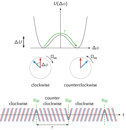
Methods Fig. S7: Noise-activated chirality inversion.

VIII Exceptional transition in a non-reciprocal O(3)-symmetric system

In this section, we discuss an example of an exceptional transition in a different symmetry group, namely the group of three-dimensional rotations $O(3)$. This supports the suggestion that exceptional transitions are a generic phenomenon not limited only to $O(2)$-equivariant systems (note, however, that $O(2)$ is indeed a subgroup of $O(3)$).

The dynamical system

$$\partial_{t}\vec{v}_{a}=\alpha_{ab}\vec{v}_{b}+\beta_{abcd}\braket{\vec{v}_{b},\vec{v}_{c}}\vec{v}_{d}$$ (S293)

in which $\vec{v}_{a}(t)$ is now an element of $\mathbb{R}^{3}$ is $O(3)$-equivariant (with the standard diagonal action). For concreteness, we use the same $\alpha_{ab}$ and $\beta_{abcd}$ as in the flocking system, and write

$$\partial_{t}\vec{v}_{A}=\left[j_{AA}\rho_{A}-\eta-\frac{1}{2\eta}\lVert j_{AA}\vec{v}_{A}+j_{AB}\vec{v}_{B}\rVert^{2}\right]\vec{v}_{A}+j_{AB}\rho_{A}\vec{v}_{B}$$ (S294)

in which the vectors are now 3D. We define $j_{\pm}=[j_{AB}\pm j_{BA}]/2$.

Direct simulations of this dynamical system show that it exhibits a time-independent phase in which the $O(3)$ symmetry is spontaneously broken: $\vec{v}_{A}$ and $\vec{v}_{B}$ acquire a finite value (and point in the same direction). This phase is destabilized by non-reciprocal interactions. We observe a transition to a chiral phase, in which the order parameters $\vec{v}_{A}(t)$ and $\vec{v}_{B}(t)$ rotate in a common plane (which plane, and in which direction is random). This transition is marked by an exceptional point at $s\equiv\sigma+\text{i}\omega=0$ in the spectrum of the Jacobian $L$ of the dynamical system, as we show in Fig. S8.

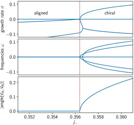
Methods Fig. S8: Exceptional transition in a O(3)-symmetric system. The spectrum of the Jacobian $L$ corresponding to Eq. (S294) exhibits an exceptional point at the transition between static alignment and chiral motion in which the order parameters orbit in the same plane, with a fixed angle between them. The two most unstable distinct eigenvalues $\lambda_{i}=\sigma_{i}+\text{i}\omega_{i}$ of $L$ coalesce at $j_{-}\approx$0.36$$. In the aligned phase, they correspond to Goldstone modes (with $\lambda=0$ in the whole phase) and massive (i.e., damped) modes. This value coincides with the transition (marked by a red dashed line) from a constant solution to a traveling waves state in which both order parameters rotate in a common plane. (Note the presence of other exceptional points with finite eigenvalues (away from the red dashed line): they are irrelevant in this discussion.) We also show the absolute value of the angle between $\vec{v}_{A}$ and $\vec{v}_{B}$. We have set $j_{AA}=j_{BB}=$1$$, $\rho_{A}=\rho_{B}=$1$$, $\eta=$0.5$$, and $j_{+}=$0.05$$.

IX Exceptional transition in coupled lasers

In this section, we discuss an example of single-body exceptional transition in laser physics and its destabilisation by the noise.

In exceptional point lasers, the main idea is to start with a linear system (e.g., coupled cavities) exhibiting an exceptional point, on top of which a lasing transition occurs. When the EP is close to the laser threshold, various interesting phenomena occur Miri and Alù (2019); Konotop et al. (2016); Feng et al. (2014); Peng et al. (2014); Brandstetter et al. (2014); Hodaei et al. (2014); Liertzer et al. (2012); Lumer et al. (2013); Hassan et al. (2015). Most of the initial literature focuses on linear models Konotop et al. (2016), with non-linearities playing essentially no role beyond determining the amplitude of the lasing emission Liertzer et al. (2012). For instance, the EP identified in Ref. Liertzer et al. (2012) occurs below the laser threshold (see Fig. 2 in Ref. Liertzer et al. (2012)). The dramatic effects of EP on the lasing transition are not related with the exceptional transitions analyzed in this paper (this can be understood as follows: the lasing transition, by which the $U(1)$ phase symmetry is spontaneously broken, should be compared to the flocking transition, or more generally the disorder-to-(anti)aligned transition).

Further studies analyzed the non-linear behavior of lasers (after threshold), see e.g. Refs Lumer et al. (2013); Hassan et al. (2015); Konotop et al. (2016). In Ref. Hassan et al. (2015), a secondary threshold was predicted and observed, which coincides with what we call exceptional transitions, as we now discuss.

Ref. Hassan et al. (2015) considers two coupled ring-shaped laser cavities. The evolution of the (nondimensionalized) complex amplitudes of light in each cavity $A_{1}$ and $A_{2}$ is described by

$$\partial_{t}A_{1} =-\gamma A_{1}+g_{0}\,\frac{A_{1}}{1+|A_{1}|^{2}}+\text{i}A_{2}$$ (S295a)

$$\partial_{t}A_{2} =-\gamma A_{2}-f_{0}\,\frac{A_{1}}{1+|A_{2}|^{2}}+\text{i}A_{1}$$ (S295b)

(the quantities called $A_{1}$ and $A_{2}$ here are called $a_{1}$ and $a_{2}$ in Eq. (3) of Ref. Hassan et al. (2015)). The linear system obtained by setting $|A_{1}|^{2}=0=|A_{2}|^{2}$ in Eq. (S295) (i.e., linerizing around $A_{1}=A_{2}=0$) has an EP when $|f_{0}+g_{0}|=2$. The lasing transition occurs when the complex amplitudes $A_{a}$ acquire a finite value, spontaneously breaking the $U(1)$ symmetry $A_{a}\to\text{e}^{\text{i}\theta}A_{a}$ (see e.g. Ref. DeGiorgio and Scully (1970); Graham and Haken (1970); Haken (1975); Gartner (2019)). From our perspective, the square-root bifurcation of the steady-state frequency $\Omega_{\text{ss}}$ (called $\lambda$ in Fig. 5 of Ref. Hassan et al. (2015)) corresponds to an exceptional transition. This can be seen by computing the eigenvalues of the Jacobian of the dynamical system in Eq. (S295), see Fig. S9. We point out that this transition is not associated with an EP of Eq. (S295) linerized around $A_{1}=A_{2}=0$ (because it is a secondary bifurcation on top of the symmetry-broken state). (In the current case, it does however coincide with an EP of the nonlinear Hamiltonian, see the discussion in section III.2.2.)

In Ref. Hassan et al. (2015), an experiment is carried out in which a transition is observed from one to two peaks in the emission spectrum of the laser (Fig. 8b and c of Ref. Hassan et al. (2015)). The two resonances in the equivalent of the chiral phase is attributed to the noise, that excites the two clockwise and counterclockwise modes (in blue and red in Fig. 5 of Ref. Hassan et al. (2015)). Because of the noise, the clockwise/counterclockwise symmetry is restored on average. We interpret this in terms of noise-assisted chirality flips in Sec. VII, in which we show that the lifetime of the chiral phase (without flips) can be exponentially enhanced by many-body effects. In principle, this could also be realized in non-Hermitian versions of photonic networks containing many coupled lasers Nixon et al. (2013); Pal et al. (2017); Mahler et al. (2020); Parto et al. (2020); Ramos et al. (2020); Honari-Latifpour and Miri (2020a, b); Acebrón et al. (2005). A similar phenomenon can also occur in quantum polariton lasers Hanai et al. (2019).

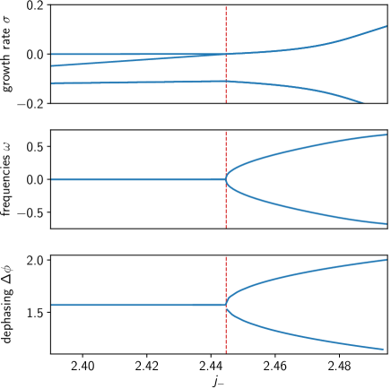
Methods Fig. S9: Exceptional transition in a coupled laser cavities. The spectrum of the Jacobian $L$ corresponding to Eq. (S295) exhibits an exceptional point at the transition between two different lasing phases, corresponding to the aligned and chiral phases. In the aligned lasing phase, the phases $\phi_{1}$ and $\phi_{2}$ of the complex amplitudes $A_{1}$ and $A_{2}$ described by Eq. (S295) are constant, while they increase or decrease at constant rate in the chiral phase (depending on the branch). The transition between these two phases is marked by a red dashed line. The two most unstable distinct eigenvalues $\lambda_{i}=\sigma_{i}+\text{i}\omega_{i}$ of $L$ coalesce at $g_{0}\approx$2.44$$. In the aligned phase, they correspond to the Goldstone mode of the broken $U(1)$ symmetry (with $\lambda=0$ in the whole phase) and a massive (i.e., damped) mode. We also show the absolute value of the angle between $\vec{v}_{A}$ and $\vec{v}_{B}$, which bifurcates into two branches in the chiral phase. The frequency of the steady-state in the chiral phase also undergoes a pitchfork bifurcation (not shown here, see Fig. 5 of Ref. Hassan et al. (2015)). We have set $f_{0}=$2$$ and $\gamma=$0.1$$, following Fig. 5 of Ref. Hassan et al. (2015).

X The case of multiple populations

In this section, we discuss the case of systems composed of more than two species interacting non-reciprocally. Most of the time, we expect their properties to reduce to the case of two species. This is because the phase transitions (bifurcations) involve only the one or two most unstable modes. For instance, the chiral phase occurs when a damped transverse mode coalesce with a Goldstone mode (see Sec. III.2.2), while the swap phase emerges when the damping rate of a longitudinal mode vanishes. These phase transitions should occur even when more than two populations are involved, provided that the most unstable modes correspond to the ones described above, while the other modes are more damped and effectively irrelevant.

That being said, richer behaviors may possibly arise when collective modes unique to multi-species systems become unstable. For example, we expect an additional phase transition within the chiral phase to arise when the third transverse mode (which do not exist in the two-species system) becomes unstable. (We order the modes by decreasing non-positive growth rate.) There, the three transverse modes are expected to affect each other non-reciprocally, which may potentially give rise to a more complex time-dependent phase in the order parameter dynamics, that might include chaotic behavior. Another possibility is the emergence of higher-order exceptional points (see e.g. Ref. Ashida et al. (2020)), where more than two eigenmodes coalesce simultaneously (corresponding to a Jordan block of size $n>2$), which may arise at higher codimension. From the point of view of bifurcation theory, this would be a special case of a Takens-Bogdanov type bifurcation with higher codimension as described in Ref. Govaerts (1993). In the vicinity of a $n$-th order exceptional point (where $n$ modes coalesce), the eigenvalues typically behave as $s\sim\text{i}\text{e}^{\text{i}2\pi m/n}\Delta^{1/n}$ ($m=0,1,\dots,n-1$), where $\Delta$ characterizes the distance from the exceptional point. As a result, we expect a higher-order exceptional point enforced pattern formation to occur in spatially extended many-body systems, even in systems without flow (where there is no convective terms). This is because the dispersion relation is expected to take the form $s(\bm{k})\sim\text{i}\text{e}^{\text{i}2\pi m/n}\bm{k}^{2/n}$ at the $n$-th order exceptional point (note that the finite $\bm{k}$ contribution $\Delta\sim\bm{k}^{2}$ characterizes the distance from the exceptional point). Hence, a dynamical instability with the growth rate $\sigma(\bm{k})=\text{Re}\,s(\bm{k})>0$ should emerge at finite momentum for $n\geq 3$. This is in contrast to the ($n=2$) exceptional point enforced pattern formation discussed in Sec. III.2.5, where the convective term of the flocking model plays an essential role. Finally, the higher-order exceptional point (with a higher codimension) could give rise to different types of phase transitions with more complicated hysteretic behavior.

XI Pattern formation in the incompressible regime

In this section, we discuss the influence of the incompressibility constraint on pattern formation. In the main text, we have entirely ignored the incompressibility constraint $\operatorname{div}(\vec{v}_{a})=0$ that would arise from Eq. (S42) in a system where mass is conserved, while still assuming constant densities $\rho_{a}\approx\text{const.}$ in order to focus on the single hydrodynamic equation (S62).

We now show that the exceptional point enforced pattern formation (discussed in Sec. III.2.5) still occurs when the incompressibility constraint $\operatorname{div}(\vec{v}_{a})=0$ is enforced.

To do so, we project the hydrodynamic equation onto the subspace of divergence-free fields. At the level of the linear stability analysis, this is done by applying the Leray projector Leray (1934); Ożański and Pooley (2017) on the Jacobian $L(k)$.

The situation where the fluid is really incompressible can be analyzed by projecting the hydrodynamic equation onto the subspace of divergence-free fields. At the level of the linear stability analysis, we use the Leray projector $\mathscr{P}(k)=\text{Id}-\ket{\hat{k}}\!\bra{\hat{k}}$ (where $\hat{k}=\vec{k}/\lVert\vec{k}\rVert$), see Refs. Leray (1934); Ożański and Pooley (2017), and consider the projected linear operator

$$L_{\text{incomp.}}(k)=\mathscr{P}(k)L(k)\mathscr{P}(k)$$ (S296)

restricted to the range of the orthogonal projection. We find that the exceptional-point-driven instability predicted in the main text is still present in the linear stability analysis of the incompressible fluid, while some of the other instabilities can disappear (see Fig. S11 and SI Movie 5). We have also performed simulations of the full hydrodynamic equation (S62) in the incompressible case (as in the main text, the simulations are performed under periodic boundary conditions using the open-source pseudospectral solver Dedalus Burns et al. (2020)). To do so, two pressure fields $\Pi_{a}$ are added as Lagrange multipliers of the incompressibility constraints. Accordingly, we added a term $-\nabla\Pi_{a}$ to the RHS of the equation of motion for $\vec{v}_{a}$. The simulations confirm the existence of pattern formation beyond the linear stability analysis, but the patterns are different, see Fig. S10).

We compare both situations in Figs. S10 and S11, that respectively show the results of simulations of the non-linear hydrodynamic theory, and the corresponding linear stability analysis of the uniform flow.

In both cases, it is unclear whether the pattern will stabilize at long times. Interestingly, we find indications that stable or metastable lattices of vortices (somewhat similar to Abrikosov lattices) can occur in some situations. These questions will be analyzed elsewhere.

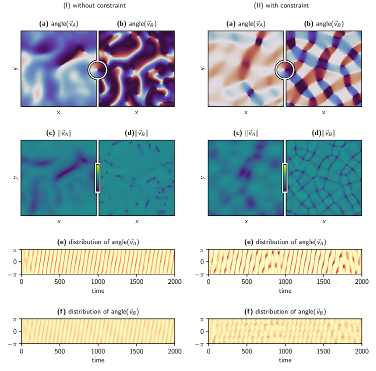
Methods Fig. S10: Pattern formation without and with incompressibility constraint We used the same parameters as in Fig. 3d-f of the main text.

Methods Fig. S11: Linear stability analysis without and with incompressibility constraint We used the same parameters as in Fig. 3d-f of the main text.

References

- Dayan and Abbott (2001) P. Dayan and L. Abbott, Theoretical neuroscience: Computational and mathematical Modelling of neural systems (MIT Press, 2001).
- Amir et al. (2016) A. Amir, N. Hatano, and D. R. Nelson, Non-hermitian localization in biological networks, Physical Review E 93, 042310 (2016).
- Krakauer et al. (2017) J. W. Krakauer, A. A. Ghazanfar, A. Gomez-Marin, M. A. MacIver, and D. Poeppel, Neuroscience needs behavior: Correcting a reductionist bias, Neuron 93, 480 (2017).
- Montbrió and Pazó (2018) E. Montbrió and D. Pazó, Kuramoto model for excitation-inhibition-based oscillations, Physical Review Letters 120, 244101 (2018).
- Parisi (1986) G. Parisi, Journal of Physics A: Mathematical and General 19, L675 (1986).
- Derrida et al. (1987) B. Derrida, E. Gardner, and A. Zippelius, An exactly solvable asymmetric neural network model, Europhysics Letters (EPL) 4, 167 (1987).
- Sompolinsky and Kanter (1986) H. Sompolinsky and I. Kanter, Temporal association in asymmetric neural networks, Physical Review Letters 57, 2861 (1986).
- Cross and Hohenberg (1993) M. C. Cross and P. C. Hohenberg, Pattern formation outside of equilibrium, Reviews of Modern Physics 65, 851 (1993).
- Marchetti et al. (2013) M. C. Marchetti, J. F. Joanny, S. Ramaswamy, T. B. Liverpool, J. Prost, M. Rao, and R. A. Simha, Hydrodynamics of soft active matter, Reviews of Modern Physics 85, 1143 (2013).
- Kotwal et al. (2019) T. Kotwal, H. Ronellenfitsch, F. Moseley, A. Stegmaier, R. Thomale, and J. Dunkel, Active topolectrical circuits (2019), arXiv:1903.10130 .
- Bricard et al. (2013) A. Bricard, J.-B. Caussin, N. Desreumaux, O. Dauchot, and D. Bartolo, Emergence of macroscopic directed motion in populations of motile colloids, Nature 503, 95 (2013).
- Palacci et al. (2013) J. Palacci, S. Sacanna, A. P. Steinberg, D. J. Pine, and P. M. Chaikin, Living crystals of light-activated colloidal surfers, Science 339, 936 (2013).
- Geyer et al. (2018) D. Geyer, A. Morin, and D. Bartolo, Sounds and hydrodynamics of polar active fluids, Nature Materials 17, 789 (2018).
- Bain and Bartolo (2019) N. Bain and D. Bartolo, Dynamic response and hydrodynamics of polarized crowds, Science 363, 46 (2019).
- van Zuiden et al. (2016) B. C. van Zuiden, J. Paulose, W. T. M. Irvine, D. Bartolo, and V. Vitelli, Spatiotemporal order and emergent edge currents in active spinner materials, Proceedings of the National Academy of Sciences 113, 12919 (2016).
- Caussin et al. (2014) J.-B. Caussin, A. Solon, A. Peshkov, H. Chaté, T. Dauxois, J. Tailleur, V. Vitelli, and D. Bartolo, Emergent spatial structures in flocking models: A dynamical system insight, Physical Review Letters 112, 148102 (2014).
- Fleury et al. (2014) R. Fleury, D. L. Sounas, C. F. Sieck, M. R. Haberman, and A. Alù, Sound isolation and giant linear nonreciprocity in a compact acoustic circulator, Science 343, 516 (2014).
- Estep et al. (2014) N. A. Estep, D. L. Sounas, J. Soric, and A. Alù, Magnetic-free non-reciprocity and isolation based on parametrically modulated coupled-resonator loops, Nature Physics 10, 923 (2014).
- Coulais et al. (2017) C. Coulais, D. Sounas, and A. Alù, Static non-reciprocity in mechanical metamaterials, Nature 542, 461 (2017).
- Miri and Alù (2019) M.-A. Miri and A. Alù, Exceptional points in optics and photonics, Science 363, eaar7709 (2019).
- Scheibner et al. (2020a) C. Scheibner, A. Souslov, D. Banerjee, P. Surówka, W. T. M. Irvine, and V. Vitelli, Odd elasticity, Nature Physics 10.1038/s41567-020-0795-y (2020a).
- Ghatak et al. (2019) A. Ghatak, M. Brandenbourger, J. van Wezel, and C. Coulais, Observation of non-hermitian topology and its bulk-edge correspondence (2019), arXiv:1907.11619 .
- Lee and Thomale (2019) C. H. Lee and R. Thomale, Anatomy of skin modes and topology in non-hermitian systems, Physical Review B 99, 201103 (2019).
- Helbig et al. (2020) T. Helbig, T. Hofmann, S. Imhof, M. Abdelghany, T. Kiessling, L. W. Molenkamp, C. H. Lee, A. Szameit, M. Greiter, and R. Thomale, Generalized bulk-boundary correspondence in non-hermitian topolectrical circuits, Nature Physics 16, 747 (2020).
- Lin et al. (2011) Z. Lin, H. Ramezani, T. Eichelkraut, T. Kottos, H. Cao, and D. N. Christodoulides, Unidirectional invisibility induced by PT-symmetric periodic structures, Physical Review Letters 106, 213901 (2011).
- Schindler et al. (2011) J. Schindler, A. Li, M. C. Zheng, F. M. Ellis, and T. Kottos, Experimental study of active LRC circuits with PT symmetries, Physical Review A 84, 040101 (2011).
- Weidemann et al. (2020) S. Weidemann, M. Kremer, T. Helbig, T. Hofmann, A. Stegmaier, M. Greiter, R. Thomale, and A. Szameit, Topological funneling of light, Science 368, 311 (2020).
- Hofmann et al. (2019) T. Hofmann, T. Helbig, C. H. Lee, M. Greiter, and R. Thomale, Chiral voltage propagation and calibration in a topolectrical chern circuit, Physical Review Letters 122, 247702 (2019).
- Brandenbourger et al. (2019) M. Brandenbourger, X. Locsin, E. Lerner, and C. Coulais, Non-reciprocal robotic metamaterials, Nature Communications 10, 10.1038/s41467-019-12599-3 (2019).
- Bender (2007) C. M. Bender, Making sense of non-hermitian hamiltonians, Reports on Progress in Physics 70, 947 (2007).
- Ramos et al. (2020) A. Ramos, L. Fernández-Alcázar, T. Kottos, and B. Shapiro, Optical phase transitions in photonic networks: a spin-system formulation, Physical Review X 10, 031024 (2020).
- Kato (1984) T. Kato, Perturbation theory for linear operators, 2nd ed. (Springer, 1984).
- Golubitsky and Stewart (2002) M. Golubitsky and I. Stewart, The Symmetry Perspective (Birkhäuser Basel, 2002).
- Crawford and Knobloch (1991) J. D. Crawford and E. Knobloch, Symmetry and symmetry-breaking bifurcations in fluid dynamics, Annual Review of Fluid Mechanics 23, 341 (1991).
- Hatano and Nelson (1996) N. Hatano and D. R. Nelson, Localization transitions in non-hermitian quantum mechanics, Physical Review Letters 77, 570 (1996).
- Bender and Boettcher (1998) C. M. Bender and S. Boettcher, Real spectra in non-hermitian hamiltonians having PT symmetry, Physical Review Letters 80, 5243 (1998).
- Nagy et al. (2010) M. Nagy, Z. Ákos, D. Biro, and T. Vicsek, Hierarchical group dynamics in pigeon flocks, Nature 464, 890 (2010).
- Morin et al. (2015) A. Morin, J.-B. Caussin, C. Eloy, and D. Bartolo, Collective motion with anticipation: Flocking, spinning, and swarming, Physical Review E 91, 012134 (2015).
- Ginelli et al. (2015) F. Ginelli, F. Peruani, M.-H. Pillot, H. Chaté, G. Theraulaz, and R. Bon, Intermittent collective dynamics emerge from conflicting imperatives in sheep herds, Proceedings of the National Academy of Sciences 112, 12729 (2015).
- Yllanes et al. (2017) D. Yllanes, M. Leoni, and M. C. Marchetti, How many dissenters does it take to disorder a flock?, New Journal of Physics 19, 103026 (2017).
- Durve et al. (2018) M. Durve, A. Saha, and A. Sayeed, Active particle condensation by non-reciprocal and time-delayed interactions, The European Physical Journal E 41, (2018).
- Barberis and Peruani (2016) L. Barberis and F. Peruani, Large-scale patterns in a minimal cognitive flocking model: Incidental leaders, nematic patterns, and aggregates, Physical Review Letters 117, 248001 (2016).
- Lavergne et al. (2019) F. A. Lavergne, H. Wendehenne, T. Bäuerle, and C. Bechinger, Group formation and cohesion of active particles with visual perception–dependent motility, Science 364, 70 (2019).
- Bonilla and Trenado (2019) L. L. Bonilla and C. Trenado, Contrarian compulsions produce exotic time-dependent flocking of active particles, Physical Review E 99, 012612 (2019).
- Costanzo (2019) A. Costanzo, Milling-induction and milling-destruction in a vicsek-like binary-mixture model, EPL (Europhysics Letters) 125, 20008 (2019).
- Dadhichi et al. (2020) L. P. Dadhichi, J. Kethapelli, R. Chajwa, S. Ramaswamy, and A. Maitra, Nonmutual torques and the unimportance of motility for long-range order in two-dimensional flocks, Physical Review E 101, 052601 (2020).
- Agudo-Canalejo and Golestanian (2019) J. Agudo-Canalejo and R. Golestanian, Active phase separation in mixtures of chemically interacting particles, Physical Review Letters 123, 018101 (2019).
- Lahiri and Ramaswamy (1997) R. Lahiri and S. Ramaswamy, Are steadily moving crystals unstable?, Physical Review Letters 79, 1150 (1997).
- Lahiri et al. (2000) R. Lahiri, M. Barma, and S. Ramaswamy, Strong phase separation in a model of sedimenting lattices, Physical Review E 61, 1648 (2000).
- Chajwa et al. (2020) R. Chajwa, N. Menon, S. Ramaswamy, and R. Govindarajan, Waves, algebraic growth and clumping in sedimenting disk arrays (2020), arXiv:2002.04168 .
- Gupta et al. (2020) R. K. Gupta, R. Kant, H. Soni, A. K. Sood, and S. Ramaswamy, Active nonreciprocal attraction between motile particles in an elastic medium (2020), arXiv:2007.04860 .
- Soto and Golestanian (2014) R. Soto and R. Golestanian, Self-assembly of catalytically active colloidal molecules: Tailoring activity through surface chemistry, Physical Review Letters 112, 068301 (2014).
- Ivlev et al. (2015) A. V. Ivlev, J. Bartnick, M. Heinen, C.-R. Du, V. Nosenko, and H. Löwen, Statistical mechanics where Newton’s third law is broken, Physical Review X 5, 011035 (2015).
- Kryuchkov et al. (2018) N. P. Kryuchkov, A. V. Ivlev, and S. O. Yurchenko, Dissipative phase transitions in systems with nonreciprocal effective interactions, Soft Matter 14, 9720 (2018).
- Saha et al. (2019) S. Saha, S. Ramaswamy, and R. Golestanian, Pairing, waltzing and scattering of chemotactic active colloids, New Journal of Physics 21, 063006 (2019).
- Maitra et al. (2020) A. Maitra, M. Lenz, and R. Voituriez, Chiral active hexatics: Giant number fluctuations, waves and destruction of order (2020), arXiv:2004.09115 .
- Uchida and Golestanian (2010) N. Uchida and R. Golestanian, Synchronization and collective dynamics in a carpet of microfluidic rotors, Physical Review Letters 104, 178103 (2010).
- Hanai et al. (2019) R. Hanai, A. Edelman, Y. Ohashi, and P. B. Littlewood, Non-hermitian phase transition from a polariton bose-einstein condensate to a photon laser, Physical Review Letters 122, 185301 (2019).
- Hanai and Littlewood (2020) R. Hanai and P. B. Littlewood, Critical fluctuations at a many-body exceptional point, Physical Review Research 2, 033018 (2020).
- Metelmann and Clerk (2015) A. Metelmann and A. A. Clerk, Nonreciprocal photon transmission and amplification via reservoir engineering, Physical Review X 5, 021025 (2015).
- Hong and Strogatz (2011a) H. Hong and S. H. Strogatz, Kuramoto model of coupled oscillators with positive and negative coupling parameters: An example of conformist and contrarian oscillators, Physical Review Letters 106, 054102 (2011a).
- Hong and Strogatz (2011b) H. Hong and S. H. Strogatz, Conformists and contrarians in a kuramoto model with identical natural frequencies, Physical Review E 84, 046202 (2011b).
- Pluchino et al. (2005) A. Pluchino, V. Latora, and A. Rapisarda, Changing opinions in a changing world: a new perspective in sociophysics, International Journal of Modern Physics C 16, 515 (2005).
- Malomed and Tribelsky (1984) B. Malomed and M. Tribelsky, Bifurcations in distributed kinetic systems with aperiodic instability, Physica D: Nonlinear Phenomena 14, 67 (1984).
- Coullet et al. (1989) P. Coullet, R. E. Goldstein, and G. H. Gunaratne, Parity-breaking transitions of modulated patterns in hydrodynamic systems, Physical Review Letters 63, 1954 (1989).
- Flesselles et al. (1991) J.-M. Flesselles, A. Simon, and A. Libchaber, Dynamics of one-dimensional interfaces: an experimentalist’s view, Advances in Physics 40, 1 (1991).
- Pan and de Bruyn (1994) L. Pan and J. R. de Bruyn, Spatially uniform traveling cellular patterns at a driven interface, Physical Review E 49, 483 (1994).
- Hohenberg and Halperin (1977) P. C. Hohenberg and B. I. Halperin, Theory of dynamic critical phenomena, Reviews of Modern Physics 49, 435 (1977).
- Kuramoto (1984) Y. Kuramoto, Chemical Oscillations, Waves, and Turbulence (Springer Berlin Heidelberg, 1984).
- Acebrón et al. (2005) J. A. Acebrón, L. L. Bonilla, C. J. P. Vicente, F. Ritort, and R. Spigler, The kuramoto model: A simple paradigm for synchronization phenomena, Reviews of Modern Physics 77, 137 (2005).
- Vicsek et al. (1995) T. Vicsek, A. Czirók, E. Ben-Jacob, I. Cohen, and O. Shochet, Novel type of phase transition in a system of self-driven particles, Physical Review Letters 75, 1226 (1995).
- Toner and Tu (1995) J. Toner and Y. Tu, Long-range order in a two-dimensional Dynamical XY Model: How birds fly together, Physical Review Letters 75, 4326 (1995).
- Daido (1992) H. Daido, Quasientrainment and slow relaxation in a population of oscillators with random and frustrated interactions, Physical Review Letters 68, 1073 (1992).
- Sakaguchi and Kuramoto (1986) H. Sakaguchi and Y. Kuramoto, A soluble active rotater model showing phase transitions via mutual entertainment, Progress of Theoretical Physics 76, 576 (1986).
- Pal et al. (2017) V. Pal, C. Tradonsky, R. Chriki, A. A. Friesem, and N. Davidson, Observing dissipative topological defects with coupled lasers, Physical Review Letters 119, 013902 (2017).
- Martens et al. (2009) E. A. Martens, E. Barreto, S. H. Strogatz, E. Ott, P. So, and T. M. Antonsen, Exact results for the kuramoto model with a bimodal frequency distribution, Physical Review E 79, 026204 (2009).
- Bonilla et al. (1998) L. Bonilla, C. P. Vicente, and R. Spigler, Time-periodic phases in populations of nonlinearly coupled oscillators with bimodal frequency distributions, Physica D: Nonlinear Phenomena 113, 79 (1998).
- Hong and Strogatz (2012) H. Hong and S. H. Strogatz, Mean-field behavior in coupled oscillators with attractive and repulsive interactions, Physical Review E 85, 056210 (2012).
- Ott and Antonsen (2008) E. Ott and T. M. Antonsen, Low dimensional behavior of large systems of globally coupled oscillators, Chaos: An Interdisciplinary Journal of Nonlinear Science 18, 037113 (2008).
- Abrams et al. (2008) D. M. Abrams, R. Mirollo, S. H. Strogatz, and D. A. Wiley, Solvable model for chimera states of coupled oscillators, Physical Review Letters 101, 084103 (2008).
- Pikovsky and Rosenblum (2008) A. Pikovsky and M. Rosenblum, Partially integrable dynamics of hierarchical populations of coupled oscillators, Physical Review Letters 101, 264103 (2008).
- Choe et al. (2016) C.-U. Choe, J.-S. Ri, and R.-S. Kim, Incoherent chimera and glassy states in coupled oscillators with frustrated interactions, Physical Review E 94, 032205 (2016).
- Gallego et al. (2017) R. Gallego, E. Montbrió, and D. Pazó, Synchronization scenarios in the winfree model of coupled oscillators, Physical Review E 96, 042208 (2017).
- O’Keeffe et al. (2017) K. P. O’Keeffe, H. Hong, and S. H. Strogatz, Oscillators that sync and swarm, Nature Communications 8, (2017).
- Levis et al. (2019) D. Levis, I. Pagonabarraga, and B. Liebchen, Activity induced synchronization: Mutual flocking and chiral self-sorting, Physical Review Research 1, 023026 (2019).
- Das et al. (2002) J. Das, M. Rao, and S. Ramaswamy, Driven heisenberg magnets: Nonequilibrium criticality, spatiotemporal chaos and control, Europhysics Letters (EPL) 60, 418 (2002).
- Das et al. (2004) J. Das, M. Rao, and S. Ramaswamy, Nonequilibrium steady states of the isotropic classical magnet (2004), arXiv:cond-mat/0404071 .
- Matheny et al. (2019) M. H. Matheny, J. Emenheiser, W. Fon, A. Chapman, A. Salova, M. Rohden, J. Li, M. H. de Badyn, M. Pósfai, L. Duenas-Osorio, M. Mesbahi, J. P. Crutchfield, M. C. Cross, R. M. D’Souza, and M. L. Roukes, Exotic states in a simple network of nanoelectromechanical oscillators, Science 363, eaav7932 (2019).
- Swift and Hohenberg (1977) J. Swift and P. C. Hohenberg, Hydrodynamic fluctuations at the convective instability, Physical Review A 15, 319 (1977).
- Rabaud et al. (1990) M. Rabaud, S. Michalland, and Y. Couder, Dynamical regimes of directional viscous fingering: Spatiotemporal chaos and wave propagation, Physical Review Letters 64, 184 (1990).
- Cummins et al. (1993) H. Z. Cummins, L. Fourtune, and M. Rabaud, Successive bifurcations in directional viscous fingering, Physical Review E 47, 1727 (1993).
- Bellon et al. (1998) L. Bellon, L. Fourtune, V. T. Minassian, and M. Rabaud, Wave-number selection and parity-breaking bifurcation in directional viscous fingering, Physical Review E 58, 565 (1998).
- Simon et al. (1988) A. J. Simon, J. Bechhoefer, and A. Libchaber, Solitary modes and the eckhaus instability in directional solidification, Physical Review Letters 61, 2574 (1988).
- Melo and Oswald (1990) F. Melo and P. Oswald, Destabilization of a faceted smectic-A–smectic-B interface, Physical Review Letters 64, 1381 (1990).
- Oswald et al. (1987) P. Oswald, J. Bechhoefer, and A. Libchaber, Instabilities of a moving nematic-isotropic interface, Physical Review Letters 58, 2318 (1987).
- Faivre et al. (1989) G. Faivre, S. de Cheveigne, C. Guthmann, and P. Kurowski, Solitary tilt waves in thin lamellar eutectics, Europhysics Letters (EPL) 9, 779 (1989).
- Faivre and Mergy (1992) G. Faivre and J. Mergy, Dynamical wavelength selection by tilt domains in thin-film lamellar eutectic growth, Physical Review A 46, 963 (1992).
- Kassner and Misbah (1990) K. Kassner and C. Misbah, Parity breaking in eutectic growth, Physical Review Letters 65, 1458 (1990).
- Ginibre et al. (1997) M. Ginibre, S. Akamatsu, and G. Faivre, Experimental determination of the stability diagram of a lamellar eutectic growth front, Physical Review E 56, 780 (1997).
- Counillon et al. (1997) C. Counillon, L. Daudet, T. Podgorski, M. C. Jullien, S. Akamatsu, and L. Limat, Global drift of a circular array of liquid columns, Europhysics Letters (EPL) 40, 37 (1997).
- Brunet et al. (2001) P. Brunet, J.-M. Flesselles, and L. Limat, Parity breaking in a one-dimensional pattern: A quantitative study with controlled wavelength, Europhysics Letters (EPL) 56, 221 (2001).
- Villain et al. (1980) J. Villain, R. Bidaux, J.-P. Carton, and R. Conte, Order as an effect of disorder, Journal de Physique 41, 1263 (1980).
- Hassan et al. (2015) A. U. Hassan, H. Hodaei, M.-A. Miri, M. Khajavikhan, and D. N. Christodoulides, Nonlinear reversal of the pt-symmetric phase transition in a system of coupled semiconductor microring resonators, Physical Review A 92, 063807 (2015).
- Liertzer et al. (2012) M. Liertzer, L. Ge, A. Cerjan, A. D. Stone, H. E. Türeci, and S. Rotter, Pump-induced exceptional points in lasers, Physical Review Letters 108, 173901 (2012).
- Lumer et al. (2013) Y. Lumer, Y. Plotnik, M. C. Rechtsman, and M. Segev, Nonlinearly induced pt transition in photonic systems, Physical Review Letters 111, 263901 (2013).
- Nixon et al. (2013) M. Nixon, E. Ronen, A. A. Friesem, and N. Davidson, Observing geometric frustration with thousands of coupled lasers, Physical Review Letters 110, 184102 (2013).
- Mahler et al. (2020) S. Mahler, M. L. Goh, C. Tradonsky, A. A. Friesem, and N. Davidson, Improved phase locking of laser arrays with nonlinear coupling, Physical Review Letters 124, 133901 (2020).
- Parto et al. (2020) M. Parto, W. Hayenga, A. Marandi, D. N. Christodoulides, and M. Khajavikhan, Realizing spin hamiltonians in nanoscale active photonic lattices, Nature Materials 19, 725 (2020).
- Honari-Latifpour and Miri (2020a) M. Honari-Latifpour and M.-A. Miri, Mapping the xy hamiltonian onto a network of coupled lasers (2020a), arXiv:2009.05091 .
- Honari-Latifpour and Miri (2020b) M. Honari-Latifpour and M.-A. Miri, Optical potts machine through networks of three-photon down-conversion oscillators, Nanophotonics 9, 4199 (2020b).
- Kuznetsov (2004) Y. A. Kuznetsov, Elements of Applied Bifurcation Theory (Springer New York, 2004).
- Shapere and Wilczek (2012) A. Shapere and F. Wilczek, Classical time crystals, Physical Review Letters 109, 160402 (2012).
- Wilczek (2012) F. Wilczek, Quantum time crystals, Physical Review Letters 109, 160401 (2012).
- Khemani et al. (2019) V. Khemani, R. Moessner, and S. L. Sondhi, A brief history of time crystals (2019), arXiv:1910.10745 .
- Yao and Nayak (2018) N. Y. Yao and C. Nayak, Time crystals in periodically driven systems, Physics Today 71, 40 (2018).
- Prigogine and Lefever (1968) I. Prigogine and R. Lefever, Symmetry breaking instabilities in dissipative systems. II, The Journal of Chemical Physics 48, 1695 (1968).
- Winfree (2001) A. T. Winfree, The Geometry of Biological Time (Springer New York, 2001).
- Giergiel et al. (2018) K. Giergiel, A. Miroszewski, and K. Sacha, Time crystal platform: From quasicrystal structures in time to systems with exotic interactions, Physical Review Letters 120, 140401 (2018).
- Autti et al. (2018) S. Autti, V. Eltsov, and G. Volovik, Observation of a time quasicrystal and its transition to a superfluid time crystal, Physical Review Letters 120, 215301 (2018).
- Mostafazadeh (2002a) A. Mostafazadeh, Pseudo-hermiticity versus PT symmetry: The necessary condition for the reality of the spectrum of a non-hermitian hamiltonian, Journal of Mathematical Physics 43, 205 (2002a).
- You et al. (2020) Z. You, A. Baskaran, and M. C. Marchetti, Nonreciprocity as a generic route to traveling states (2020), arXiv:2005.07684 .
- Saha et al. (2020) S. Saha, J. Agudo-Canalejo, and R. Golestanian, Scalar active mixtures: The non-reciprocal cahn-hilliard model (2020), arXiv:2005.07101 .
- Trefethen and Embree (2005) L. N. Trefethen and M. Embree, Spectra and Pseudospectra (Princeton University Press, 2005).
- Trefethen et al. (1993) L. N. Trefethen, A. E. Trefethen, S. C. Reddy, and T. A. Driscoll, Hydrodynamic stability without eigenvalues, Science 261, 578 (1993).
- Grossmann (2000) S. Grossmann, The onset of shear flow turbulence, Reviews of Modern Physics 72, 603 (2000).
- Chomaz (2005) J.-M. Chomaz, Global instabilities in spatially developing flows: Non-normality and nonlinearity, Annual Review of Fluid Mechanics 37, 357 (2005).
- Schmid (2007) P. J. Schmid, Nonmodal stability theory, Annual Review of Fluid Mechanics 39, 129 (2007).
- Murphy and Miller (2009) B. K. Murphy and K. D. Miller, Balanced amplification: A new mechanism of selective amplification of neural activity patterns, Neuron 61, 635 (2009).
- Hennequin et al. (2012) G. Hennequin, T. P. Vogels, and W. Gerstner, Non-normal amplification in random balanced neuronal networks, Physical Review E 86, 011909 (2012).
- Asllani and Carletti (2018) M. Asllani and T. Carletti, Topological resilience in non-normal networked systems, Physical Review E 97, 042302 (2018).
- Asllani et al. (2018) M. Asllani, R. Lambiotte, and T. Carletti, Structure and dynamical behavior of non-normal networks, Science Advances 4, eaau9403 (2018).
- Baggio et al. (2020) G. Baggio, V. Rutten, G. Hennequin, and S. Zampieri, Efficient communication over complex dynamical networks: The role of matrix non-normality, Science Advances 6, eaba2282 (2020).
- Nicolaou et al. (2020) Z. G. Nicolaou, T. Nishikawa, S. B. Nicholson, J. R. Green, and A. E. Motter, Non-normality and non-monotonic dynamics in complex reaction networks (2020), arXiv:2008.09616v1 .
- Neubert and Caswell (1997) M. G. Neubert and H. Caswell, Alternatives to resilience for measuring the responses of ecological systems to perturbations, Ecology 78, 653 (1997).
- Nelson and Shnerb (1998) D. R. Nelson and N. M. Shnerb, Non-hermitian localization and population biology, Physical Review E 58, 1383 (1998).
- Neubert et al. (2004) M. G. Neubert, T. Klanjscek, and H. Caswell, Reactivity and transient dynamics of predator–prey and food web models, Ecological Modelling 179, 29 (2004).
- Townley et al. (2007) S. Townley, D. Carslake, O. Kellie-smith, D. Mccarthy, and D. Hodgson, Predicting transient amplification in perturbed ecological systems, Journal of Applied Ecology 44, 1243 (2007).
- Ridolfi et al. (2011) L. Ridolfi, C. Camporeale, P. D’Odorico, and F. Laio, Transient growth induces unexpected deterministic spatial patterns in the turing process, EPL (Europhysics Letters) 95, 18003 (2011).
- Biancalani et al. (2017) T. Biancalani, F. Jafarpour, and N. Goldenfeld, Giant amplification of noise in fluctuation-induced pattern formation, Physical Review Letters 118, 018101 (2017).
- Feng et al. (2017) L. Feng, R. El-Ganainy, and L. Ge, Non-hermitian photonics based on parity–time symmetry, Nature Photonics 11, 752 (2017).
- Ashida et al. (2020) Y. Ashida, Z. Gong, and M. Ueda, Non-hermitian physics (2020), arXiv:2006.01837v1 .
- Ashida et al. (2017) Y. Ashida, S. Furukawa, and M. Ueda, Parity-time-symmetric quantum critical phenomena, Nature Communications 8, 10.1038/ncomms15791 (2017).
- Tripathi et al. (2016) V. Tripathi, A. Galda, H. Barman, and V. M. Vinokur, Parity-time symmetry-breaking mechanism of dynamic mott transitions in dissipative systems, Physical Review B 94, 041104 (2016).
- Bernier et al. (2014) N. R. Bernier, E. G. D. Torre, and E. Demler, Unstable avoided crossing in coupled spinor condensates, Physical Review Letters 113, 065303 (2014).
- Aharonyan and Torre (2019) M. Aharonyan and E. G. D. Torre, Many-body exceptional points in colliding condensates, Molecular Physics 117, 1971 (2019).
- Newton (1687) I. Newton, Philosophiæ Naturalis Principia Mathematica (1687).
- Ermak and McCammon (1978) D. L. Ermak and J. A. McCammon, Brownian dynamics with hydrodynamic interactions, The Journal of Chemical Physics 69, 1352 (1978).
- Leonardo et al. (2008) R. D. Leonardo, S. Keen, F. Ianni, J. Leach, M. J. Padgett, and G. Ruocco, Hydrodynamic interactions in two dimensions, Physical Review E 78, 031406 (2008).
- Dholakia and Zemánek (2010) K. Dholakia and P. Zemánek, Colloquium: Gripped by light: Optical binding, Reviews of Modern Physics 82, 1767 (2010).
- Yifat et al. (2018) Y. Yifat, D. Coursault, C. W. Peterson, J. Parker, Y. Bao, S. K. Gray, S. A. Rice, and N. F. Scherer, Reactive optical matter: light-induced motility in electrodynamically asymmetric nanoscale scatterers, Light: Science & Applications 7, 10.1038/s41377-018-0105-y (2018).
- Peterson et al. (2019) C. W. Peterson, J. Parker, S. A. Rice, and N. F. Scherer, Controlling the dynamics and optical binding of nanoparticle homodimers with transverse phase gradients, Nano Letters 19, 897 (2019).
- Rosa and Ruzzene (2020) M. I. N. Rosa and M. Ruzzene, Dynamics and topology of non-hermitian elastic lattices with non-local feedback control interactions, New Journal of Physics 22, 053004 (2020).
- Chen et al. (2020) Y. Chen, X. Li, C. Scheibner, V. Vitelli, and G. Huang, Self-sensing metamaterials with odd micropolarity (2020), arXiv:2009.07329 .
- Tasaki (2020) H. Tasaki, Hohenberg-mermin-wagner type theorems for equilibrium models of flocking (2020), arXiv:2008.02698v2 .
- Fodor et al. (2016) É. Fodor, C. Nardini, M. E. Cates, J. Tailleur, P. Visco, and F. van Wijland, How far from equilibrium is active matter?, Physical Review Letters 117, 038103 (2016).
- Loos and Klapp (2020) S. A. M. Loos and S. H. L. Klapp, Thermodynamic implications of non-reciprocity (2020), arXiv:2008.00894v1 .
- Loos et al. (2019) S. A. M. Loos, S. M. Hermann, and S. H. L. Klapp, Non-reciprocal hidden degrees of freedom: A unifying perspective on memory, feedback, and activity (2019), arXiv:1910.08372v1 .
- Malzard et al. (2015) S. Malzard, C. Poli, and H. Schomerus, Topologically protected defect states in open photonic systems with non-hermitian charge-conjugation and parity-time symmetry, Physical Review Letters 115, 200402 (2015).
- Lee et al. (2020) C. H. Lee, L. Li, R. Thomale, and J. Gong, Unraveling non-hermitian pumping: Emergent spectral singularities and anomalous responses, Physical Review B 102, 085151 (2020).
- Okuma et al. (2020) N. Okuma, K. Kawabata, K. Shiozaki, and M. Sato, Topological origin of non-hermitian skin effects, Physical Review Letters 124, 086801 (2020).
- Lee et al. (2019) C. H. Lee, L. Li, and J. Gong, Hybrid higher-order skin-topological modes in nonreciprocal systems, Physical Review Letters 123, 016805 (2019).
- Zhang et al. (2020) K. Zhang, Z. Yang, and C. Fang, Correspondence between winding numbers and skin modes in non-hermitian systems, Physical Review Letters 125, 126402 (2020).
- Achenbach (2004) J. D. Achenbach, Reciprocity in Elastodynamics (Cambridge University Press, 2004).
- Nassar et al. (2020) H. Nassar, B. Yousefzadeh, R. Fleury, M. Ruzzene, A. Alù, C. Daraio, A. N. Norris, G. Huang, and M. R. Haberman, Nonreciprocity in acoustic and elastic materials, Nature Reviews Materials 10.1038/s41578-020-0206-0 (2020).
- Potton (2004) R. J. Potton, Reciprocity in optics, Reports on Progress in Physics 67, 717 (2004).
- Caloz et al. (2018) C. Caloz, A. Alù, S. Tretyakov, D. Sounas, K. Achouri, and Z.-L. Deck-Léger, Electromagnetic nonreciprocity, Physical Review Applied 10, 047001 (2018).
- Masoud and Stone (2019) H. Masoud and H. A. Stone, The reciprocal theorem in fluid dynamics and transport phenomena, Journal of Fluid Mechanics 879, 10.1017/jfm.2019.553 (2019).
- Scheibner et al. (2020b) C. Scheibner, W. T. M. Irvine, and V. Vitelli, Non-hermitian band topology and skin modes in active elastic media, Physical Review Letters 125, 118001 (2020b).
- Zhou and Zhang (2020) D. Zhou and J. Zhang, Non-hermitian topological metamaterials with odd elasticity, Physical Review Research 2, 023173 (2020).
- Groot and Mazur (1962) S. R. D. Groot and P. Mazur, Non-Equilibrium Thermodynamics (Dover Publications, 1962).
- Avron (1998) J. E. Avron, Journal of Statistical Physics 92, 543 (1998).
- Banerjee et al. (2017) D. Banerjee, A. Souslov, A. G. Abanov, and V. Vitelli, Odd viscosity in chiral active fluids, Nature Communications 8, (2017).
- Souslov et al. (2019) A. Souslov, K. Dasbiswas, M. Fruchart, S. Vaikuntanathan, and V. Vitelli, Topological waves in fluids with odd viscosity, Physical Review Letters 122, 128001 (2019).
- Soni et al. (2019) V. Soni, E. S. Bililign, S. Magkiriadou, S. Sacanna, D. Bartolo, M. J. Shelley, and W. T. M. Irvine, The odd free surface flows of a colloidal chiral fluid, Nature Physics 15, 1188 (2019).
- Han et al. (2020) M. Han, M. Fruchart, C. Scheibner, S. Vaikuntanathan, W. Irvine, J. de Pablo, and V. Vitelli, Statistical mechanics of a chiral active fluid (2020), arXiv:2002.07679 .
- Dean (1996) D. S. Dean, Langevin equation for the density of a system of interacting langevin processes, Journal of Physics A: Mathematical and General 29, L613 (1996).
- Bertin et al. (2006) E. Bertin, M. Droz, and G. Grégoire, Boltzmann and hydrodynamic description for self-propelled particles, Physical Review E 74, 022101 (2006).
- Bertin et al. (2009) E. Bertin, M. Droz, and G. Grégoire, Hydrodynamic equations for self-propelled particles: microscopic derivation and stability analysis, Journal of Physics A: Mathematical and Theoretical 42, 445001 (2009).
- Farrell et al. (2012) F. D. C. Farrell, M. C. Marchetti, D. Marenduzzo, and J. Tailleur, Pattern formation in self-propelled particles with density-dependent motility, Physical Review Letters 108, 248101 (2012).
- Chaté and Mahault (2019) H. Chaté and B. Mahault, Dry, aligning, dilute, active matter: A synthetic and self-contained overview (2019), arXiv:1906.05542 .
- Toner and Tu (1998) J. Toner and Y. Tu, Flocks, herds, and schools: A quantitative theory of flocking, Physical Review E 58, 4828 (1998).
- Peshkov et al. (2014) A. Peshkov, E. Bertin, F. Ginelli, and H. Chaté, Boltzmann-ginzburg-landau approach for continuous descriptions of generic vicsek-like models, The European Physical Journal Special Topics 223, 1315 (2014).
- Ihle (2011) T. Ihle, Kinetic theory of flocking: Derivation of hydrodynamic equations, Physical Review E 83, 030901 (2011).
- Mahault et al. (2019) B. Mahault, F. Ginelli, and H. Chaté, Quantitative assessment of the toner and tu theory of polar flocks, Physical Review Letters 123, 218001 (2019).
- Oza and Dunkel (2016) A. U. Oza and J. Dunkel, Antipolar ordering of topological defects in active liquid crystals, New Journal of Physics 18, 093006 (2016).
- Suzuki et al. (2015) R. Suzuki, C. A. Weber, E. Frey, and A. R. Bausch, Polar pattern formation in driven filament systems requires non-binary particle collisions, Nature Physics 11, 839 (2015).
- Nishiguchi et al. (2017) D. Nishiguchi, K. H. Nagai, H. Chaté, and M. Sano, Long-range nematic order and anomalous fluctuations in suspensions of swimming filamentous bacteria, Physical Review E 95, 020601 (2017).
- Tsai et al. (2005) J.-C. Tsai, F. Ye, J. Rodriguez, J. P. Gollub, and T. C. Lubensky, A chiral granular gas, Physical Review Letters 94, 214301 (2005).
- Liebchen and Levis (2017) B. Liebchen and D. Levis, Collective behavior of chiral active matter: Pattern formation and enhanced flocking, Physical Review Letters 119, 058002 (2017).
- Burns et al. (2020) K. J. Burns, G. M. Vasil, J. S. Oishi, D. Lecoanet, and B. P. Brown, Dedalus: A flexible framework for numerical simulations with spectral methods, Physical Review Research 2, 023068 (2020).
- Wang and Ruuth (2008) D. Wang and S. J. Ruuth, Variable step-size implicit-explicit linear multistep methods for time-dependent partial differential equations, Journal of Computational Mathematics 26, 838 (2008).
- Arnold (1988) V. I. Arnold, Geometrical Methods in the Theory of Ordinary Differential Equations (Springer New York, 1988).
- Golubitsky and Schaeffer (1985) M. Golubitsky and D. G. Schaeffer, Singularities and Groups in Bifurcation Theory, Vol. I (Springer New York, 1985).
- Golubitsky et al. (1988) M. Golubitsky, I. Stewart, and D. G. Schaeffer, Singularities and Groups in Bifurcation Theory, Vol. II (Springer New York, 1988).
- Chossat and Lauterbach (2000) P. Chossat and R. Lauterbach, Methods in Equivariant Bifurcations and Dynamical Systems (World Scientific, 2000).
- Bogdanov (1981a) R. I. Bogdanov, Bifurcations of a limit cycle for a family of vector fields on the plane, Selecta Mathematica Sovietica 1, 373 (1981a), translated from: Trudy Sem. Petrovsk. 2, 23-35 (1976).
- Bogdanov (1981b) R. I. Bogdanov, Versal deformations of a singularity of a vector field on the plane in the case of zero eigenvalues, Selecta Mathematica Sovietica 1, 389 (1981b), translated from: Trudy Sem. Petrovsk. 2, 37-65 (1976).
- Takens (1974) F. Takens, Forced oscillations and bifurcations, Communications of the Mathematical Institute Rijksuniversiteit Utrecht 3 (1974), reprinted in: Global Analysis of Dynamical Systems (IOP, ISBN 0750308036).
- Landau and Khalatnikov (1954) L. Landau and I. Khalatnikov, On the anomalous absorption of sound near a second order phase transition point, in Dokl. Akad. Nauk SSSR, Vol. 96 (1954) pp. 469–472.
- Wilson (1974) K. Wilson, The renormalization group and the epsilon expansion, Physics Reports 12, 75 (1974).
- Hohenberg and Krekhov (2015) P. Hohenberg and A. Krekhov, An introduction to the ginzburg-landau theory of phase transitions and nonequilibrium patterns, Physics Reports 572, 1 (2015).
- Hove (1954) L. V. Hove, Time-dependent correlations between spins and neutron scattering in ferromagnetic crystals, Physical Review 95, 1374 (1954).
- Laguës and Lesne (2003) M. Laguës and A. Lesne, Invariances d’échelle : des changements d’états à la turbulence (Belin, Paris, 2003).
- Muñoz (2018) M. A. Muñoz, Colloquium: Criticality and dynamical scaling in living systems, Reviews of Modern Physics 90, 031001 (2018).
- Sornette (2000) D. Sornette, Critical Phenomena in Natural Sciences (Springer Berlin Heidelberg, 2000).
- Saarloos (1994) W. v. Saarloos, The complex Ginzburg-Landau equation for beginners, in Spatio-temporal Patterns in Nonequilibrium Complex Systems, Vol. XXI, edited by P. E. Cladis and P. Palffy-Muhoray (Addison-Wesley, 1994) pp. –.
- Aranson and Kramer (2002) I. S. Aranson and L. Kramer, The world of the complex Ginzburg-Landau equation, Reviews of Modern Physics 74, 99 (2002).
- Barrat and Hansen (2003) J.-L. Barrat and J.-P. Hansen, Basic Concepts for Simple and Complex Liquids (Cambridge University Press, 2003).
- von Neumann and Wigner (1929) J. von Neumann and E. P. Wigner, Über das verhalten von eigenwerten bei adiabatischen prozessen, Physik. Z. 30, 467 (1929), translated in R. S. Knox and A. Gold, Symmetry in the Solid State (Benjamin, New York, 1964).
- Arnol’d (1972) V. I. Arnol’d, Modes and quasimodes, Functional Analysis and Its Applications 6, 94 (1972), translated from: V. I. Arnol’d, Modes and quasimodes, Funktsional. Anal. i Prilozhen., 6, 2 (1972).
- Arnold (1995) V. I. Arnold, Remarks on eigenvalues and eigenvectors of hermitian matrices, berry phase, adiabatic connections and quantum hall effect, Selecta Mathematica 1, 1 (1995).
- Seyranian et al. (2005) A. P. Seyranian, O. N. Kirillov, and A. A. Mailybaev, Coupling of eigenvalues of complex matrices at diabolic and exceptional points, Journal of Physics A: Mathematical and General 38, 1723 (2005).
- Julien (1994) K. A. Julien, Strong spatial interactions with 1:1 resonance: a three-layer convection problem, Nonlinearity 7, 1655 (1994).
- Renardy et al. (1999) Y. Y. Renardy, M. Renardy, and K. Fujimura, Takens-bogdanov bifurcation on the hexagonal lattice for double-layer convection, Physica D: Nonlinear Phenomena 129, 171 (1999).
- Guckenheimer (1986) J. Guckenheimer, A codimension two bifurcation with circular symmetry (1986).
- Dangelmayr and Knobloch (1987) G. Dangelmayr and E. Knobloch, The Takens–Bogdanov bifurcation with O(2)-symmetry, Philosophical Transactions of the Royal Society of London. Series A, Mathematical and Physical Sciences 322, 243 (1987).
- Krupa (1990) M. Krupa, Bifurcations of relative equilibria, SIAM Journal on Mathematical Analysis 21, 1453 (1990).
- Field (1980) M. J. Field, Equivariant dynamical systems, Transactions of the American Mathematical Society 259, 185 (1980).
- Nambu (1960) Y. Nambu, Quasi-Particles and Gauge Invariance in the Theory of Superconductivity, Physical Review 117, 648 (1960).
- Goldstone (1961) J. Goldstone, Field theories with Superconductor solutions, Il Nuovo Cimento 19, 154 (1961).
- Goldstone et al. (1962) J. Goldstone, A. Salam, and S. Weinberg, Broken Symmetries, Physical Review 127, 965 (1962).
- Hidaka (2013) Y. Hidaka, Counting rule for nambu-goldstone modes in nonrelativistic systems, Physical Review Letters 110, 091601 (2013).
- Watanabe (2020) H. Watanabe, Counting rules of nambu-goldstone modes, Annual Review of Condensed Matter Physics 11, 169 (2020).
- Watanabe and Murayama (2012) H. Watanabe and H. Murayama, Unified description of nambu-goldstone bosons without lorentz invariance, Physical Review Letters 108, 251602 (2012).
- Nielsen and Chadha (1976) H. Nielsen and S. Chadha, On how to count goldstone bosons, Nuclear Physics B 105, 445 (1976).
- Leroy (1992) L. Leroy, On spontaneous symmetry breakdown in dynamical systems, Journal of Physics A: Mathematical and General 25, L987 (1992).
- Minami and Hidaka (2018) Y. Minami and Y. Hidaka, Spontaneous symmetry breaking and nambu-goldstone modes in dissipative systems, Physical Review E 97, 012130 (2018).
- Hongo et al. (2019) M. Hongo, S. Kim, T. Noumi, and A. Ota, Effective Lagrangian for Nambu-Goldstone modes in nonequilibrium open systems (2019), arXiv:1907.08609 .
- Daido (1987) H. Daido, Population dynamics of randomly interacting self-oscillators. i: Tractable models without frustration, Progress of Theoretical Physics 77, 622 (1987).
- Omata et al. (1988) S. Omata, Y. Yamaguchi, and H. Shimizu, Entrainment among coupled limit cycle oscillators with frustration, Physica D: Nonlinear Phenomena 31, 397 (1988).
- Martens et al. (2016) E. A. Martens, C. Bick, and M. J. Panaggio, Chimera states in two populations with heterogeneous phase-lag, Chaos: An Interdisciplinary Journal of Nonlinear Science 26, 094819 (2016).
- Pazó and Montbrió (2009) D. Pazó and E. Montbrió, Existence of hysteresis in the kuramoto model with bimodal frequency distributions, Physical Review E 80, 046215 (2009).
- Pietras et al. (2018) B. Pietras, N. Deschle, and A. Daffertshofer, First-order phase transitions in the kuramoto model with compact bimodal frequency distributions, Physical Review E 98, 062219 (2018).
- Ott and Antonsen (2009) E. Ott and T. M. Antonsen, Long time evolution of phase oscillator systems, Chaos: An Interdisciplinary Journal of Nonlinear Science 19, 023117 (2009).
- Watanabe and Strogatz (1993) S. Watanabe and S. H. Strogatz, Integrability of a globally coupled oscillator array, Physical Review Letters 70, 2391 (1993).
- Watanabe and Strogatz (1994) S. Watanabe and S. H. Strogatz, Constants of motion for superconducting josephson arrays, Physica D: Nonlinear Phenomena 74, 197 (1994).
- Marvel et al. (2009) S. A. Marvel, R. E. Mirollo, and S. H. Strogatz, Identical phase oscillators with global sinusoidal coupling evolve by möbius group action, Chaos: An Interdisciplinary Journal of Nonlinear Science 19, 043104 (2009).
- Pikovsky and Rosenblum (2011) A. Pikovsky and M. Rosenblum, Dynamics of heterogeneous oscillator ensembles in terms of collective variables, Physica D: Nonlinear Phenomena 240, 872 (2011).
- Tyulkina et al. (2018) I. V. Tyulkina, D. S. Goldobin, L. S. Klimenko, and A. Pikovsky, Dynamics of noisy oscillator populations beyond the ott-antonsen ansatz, Physical Review Letters 120, 264101 (2018).
- Montbrió et al. (2015) E. Montbrió, D. Pazó, and A. Roxin, Macroscopic description for networks of spiking neurons, Physical Review X 5, 021028 (2015).
- Bick et al. (2020) C. Bick, M. Goodfellow, C. R. Laing, and E. A. Martens, Understanding the dynamics of biological and neural oscillator networks through exact mean-field reductions: a review (2020).
- Doppler et al. (2016) J. Doppler, A. A. Mailybaev, J. Böhm, U. Kuhl, A. Girschik, F. Libisch, T. J. Milburn, P. Rabl, N. Moiseyev, and S. Rotter, Dynamically encircling an exceptional point for asymmetric mode switching, Nature 537, 76 (2016).
- Dembowski et al. (2004) C. Dembowski, B. Dietz, H.-D. Gräf, H. L. Harney, A. Heine, W. D. Heiss, and A. Richter, Encircling an exceptional point, Physical Review E 69, 056216 (2004).
- Milburn et al. (2015) T. J. Milburn, J. Doppler, C. A. Holmes, S. Portolan, S. Rotter, and P. Rabl, General description of quasiadiabatic dynamical phenomena near exceptional points, Physical Review A 92, 052124 (2015).
- Mailybaev et al. (2005) A. A. Mailybaev, O. N. Kirillov, and A. P. Seyranian, Geometric phase around exceptional points, Physical Review A 72, 014104 (2005).
- Galda and Vinokur (2016) A. Galda and V. M. Vinokur, Parity-time symmetry breaking in magnetic systems, Physical Review B 94, 020408(R) (2016).
- Galda and Vinokur (2019) A. Galda and V. M. Vinokur, Exceptional points in classical spin dynamics, Scientific Reports 9, 10.1038/s41598-019-53455-0 (2019).
- Kepesidis et al. (2016) K. V. Kepesidis, T. J. Milburn, J. Huber, K. G. Makris, S. Rotter, and P. Rabl, Pt-symmetry breaking in the steady state of microscopic gain-loss systems, New Journal of Physics 18, 095003 (2016).
- Graefe et al. (2010) E.-M. Graefe, H. J. Korsch, and A. E. Niederle, Quantum-classical correspondence for a non-hermitian bose-hubbard dimer, Physical Review A 82, 013629 (2010).
- Cartarius et al. (2008) H. Cartarius, J. Main, and G. Wunner, Discovery of exceptional points in the bose-einstein condensation of gases with attractive1/rinteraction, Physical Review A 77, 013618 (2008).
- Gutöhrlein et al. (2013) R. Gutöhrlein, J. Main, H. Cartarius, and G. Wunner, Bifurcations and exceptional points in dipolar bose-einstein condensates, Journal of Physics A: Mathematical and Theoretical 46, 305001 (2013).
- Strack and Vitelli (2013) P. Strack and V. Vitelli, Soft quantum vibrations of a PT-symmetric nonlinear ion chain, Physical Review A 88, 053408 (2013).
- Hong (2014) H. Hong, Periodic synchronization and chimera in conformist and contrarian oscillators, Physical Review E 89, 062924 (2014).
- Kemeth et al. (2016) F. P. Kemeth, S. W. Haugland, L. Schmidt, I. G. Kevrekidis, and K. Krischer, A classification scheme for chimera states, Chaos: An Interdisciplinary Journal of Nonlinear Science 26, 094815 (2016).
- Hoyle (2006) R. Hoyle, Pattern Formation (Cambridge University Press, 2006).
- Cross and Greenside (2009) M. Cross and H. Greenside, Pattern Formation and Dynamics in Nonequilibrium Systems (Cambridge University Press, 2009).
- Meron (2015) E. Meron, Nonlinear Physics of Ecosystems (CRC Press, 2015).
- Douady et al. (1989) S. Douady, S. Fauve, and O. Thual, Oscillatory phase modulation of parametrically forced surface waves, Europhysics Letters (EPL) 10, 309 (1989).
- Coullet and Iooss (1990) P. Coullet and G. Iooss, Instabilities of one-dimensional cellular patterns, Physical Review Letters 64, 866 (1990).
- Fauve et al. (1991) S. Fauve, S. Douady, and O. Thual, Drift instabilities of cellular patterns, Journal de Physique II 1, 311 (1991).
- Coullet and Fauve (1985) P. Coullet and S. Fauve, Propagative phase dynamics for systems with galilean invariance, Physical Review Letters 55, 2857 (1985).
- Brachet et al. (1987) M. E. Brachet, P. Coullet, and S. Fauve, Propagative phase dynamics in temporally intermittent systems, Europhysics Letters (EPL) 4, 1017 (1987).
- Knobloch et al. (1995) E. Knobloch, J. Hettel, and G. Dangelmayr, Parity breaking bifurcation in inhomogeneous systems, Physical Review Letters 74, 4839 (1995).
- Armbruster et al. (1988) D. Armbruster, J. Guckenheimer, and P. Holmes, Heteroclinic cycles and modulated travelling waves in systems with o(2) symmetry, Physica D: Nonlinear Phenomena 29, 257 (1988).
- Proctor and Jones (1988) M. R. E. Proctor and C. A. Jones, The interaction of two spatially resonant patterns in thermal convection. part 1. exact 1:2 resonance, Journal of Fluid Mechanics 188, 301 (1988).
- Dangelmayr et al. (1997) G. Dangelmayr, J. Hettel, and E. Knobloch, Parity-breaking bifurcation in inhomogeneous systems, Nonlinearity 10, 1093 (1997).
- Knobloch and Proctor (1981) E. Knobloch and M. R. E. Proctor, Nonlinear periodic convection in double-diffusive systems, Journal of Fluid Mechanics 108, 291 (1981).
- Cross and Kim (1988) M. C. Cross and K. Kim, Linear instability and the codimension-2 region in binary fluid convection between rigid impermeable boundaries, Physical Review A 37, 3909 (1988).
- Cross (1986) M. C. Cross, Traveling and standing waves in binary-fluid convection in finite geometries, Physical Review Letters 57, 2935 (1986).
- Coullet and Spiegel (1983) P. H. Coullet and E. A. Spiegel, Amplitude equations for systems with competing instabilities, SIAM Journal on Applied Mathematics 43, 776 (1983).
- Cross (1988) M. C. Cross, Structure of nonlinear traveling-wave states in finite geometries, Physical Review A 38, 3593 (1988).
- Brand et al. (1983) H. R. Brand, P. C. Hohenberg, and V. Steinberg, Amplitude equation near a polycritical point for the convective instability of a binary fluid mixture in a porous medium, Physical Review A 27, 591 (1983).
- Brand et al. (1984) H. R. Brand, P. C. Hohenberg, and V. Steinberg, Codimension-2 bifurcations for convection in binary fluid mixtures, Physical Review A 30, 2548 (1984).
- Guckenheimer (1984) J. Guckenheimer, Multiple bifurcation problems of codimension two, SIAM Journal on Mathematical Analysis 15, 1 (1984).
- Moses and Steinberg (1986) E. Moses and V. Steinberg, Flow patterns and nonlinear behavior of traveling waves in a convective binary fluid, Physical Review A 34, 693 (1986).
- Walden et al. (1985) R. W. Walden, P. Kolodner, A. Passner, and C. M. Surko, Traveling waves and chaos in convection in binary fluid mixtures, Physical Review Letters 55, 496 (1985).
- Coullet et al. (1985) P. Coullet, S. Fauve, and E. Tirapegui, Large scale instability of nonlinear standing waves, Journal de Physique Lettres 46, 787 (1985).
- Bensimon et al. (1989) D. Bensimon, A. Pumir, and B. Shraiman, Nonlinear theory of traveling wave convection in binary mixtures, Journal de Physique 50, 3089 (1989).
- Knobloch and Moore (1990) E. Knobloch and D. R. Moore, Minimal model of binary fluid convection, Physical Review A 42, 4693 (1990).
- Schöpf and Zimmermann (1993) W. Schöpf and W. Zimmermann, Convection in binary fluids: Amplitude equations, codimension-2 bifurcation, and thermal fluctuations, Physical Review E 47, 1739 (1993).
- Bressloff et al. (2001) P. C. Bressloff, J. D. Cowan, M. Golubitsky, P. J. Thomas, and M. C. Wiener, Geometric visual hallucinations, euclidean symmetry and the functional architecture of striate cortex, Philosophical Transactions of the Royal Society of London. Series B: Biological Sciences 356, 299 (2001).
- Bressloff et al. (2002) P. C. Bressloff, J. D. Cowan, M. Golubitsky, P. J. Thomas, and M. C. Wiener, What geometric visual hallucinations tell us about the visual cortex, Neural Computation 14, 473 (2002).
- Cho and Kim (2004) M. W. Cho and S. Kim, Understanding visual map formation through vortex dynamics of spin hamiltonian models, Physical Review Letters 92, 018101 (2004).
- Schnabel et al. (2008) M. Schnabel, M. Kaschube, and F. Wolf, Pinwheel stability, pattern selection and the geometry of visual space (2008), arXiv:0801.3832v2 .
- Butler et al. (2011) T. C. Butler, M. Benayoun, E. Wallace, W. van Drongelen, N. Goldenfeld, and J. Cowan, Evolutionary constraints on visual cortex architecture from the dynamics of hallucinations, Proceedings of the National Academy of Sciences 109, 606 (2011).
- Curtu and Ermentrout (2004) R. Curtu and B. Ermentrout, Pattern formation in a network of excitatory and inhibitory cells with adaptation, SIAM Journal on Applied Dynamical Systems 3, 191 (2004).
- Adini et al. (1997) Y. Adini, D. Sagi, and M. Tsodyks, Excitatory-inhibitory network in the visual cortex: Psychophysical evidence, Proceedings of the National Academy of Sciences 94, 10426 (1997).
- Hensch and Fagiolini (2005) T. K. Hensch and M. Fagiolini, Excitatory-inhibitory balance and critical period plasticity in developing visual cortex, in Progress in Brain Research (Elsevier, 2005) pp. 115–124.
- Chossat and Iooss (1994) P. Chossat and G. Iooss, The Couette-Taylor Problem (Springer New York, 1994).
- Riecke and Paap (1992) H. Riecke and H.-G. Paap, Parity-breaking and hopf bifurcations in axisymmetric taylor vortex flow, Physical Review A 45, 8605 (1992).
- Tennakoon et al. (1996) S. G. K. Tennakoon, C. D. Andereck, J. J. Hegseth, and H. Riecke, Temporal modulation of traveling waves in the flow between rotating cylinders with broken azimuthal symmetry, Physical Review E 54, 5053 (1996).
- Mutabazi and Andereck (1995) I. Mutabazi and C. D. Andereck, Mode resonance and wavelength-halving instability in the taylor-dean system, Physical Review E 51, 4380 (1995).
- Bot et al. (1998) P. Bot, O. Cadot, and I. Mutabazi, Secondary instability mode of a roll pattern and transition to spatiotemporal chaos in the taylor-dean system, Physical Review E 58, 3089 (1998).
- Wiener and McAlister (1992) R. J. Wiener and D. F. McAlister, Parity breaking and solitary waves in axisymmetric taylor vortex flow, Physical Review Letters 69, 2915 (1992).
- Andereck et al. (1986) C. D. Andereck, S. S. Liu, and H. L. Swinney, Flow regimes in a circular couette system with independently rotating cylinders, Journal of Fluid Mechanics 164, 155 (1986).
- Altmeyer and Hoffmann (2010) S. Altmeyer and C. Hoffmann, Secondary bifurcation of mixed-cross-spirals connecting travelling wave solutions, New Journal of Physics 12, 113035 (2010).
- Pinter et al. (2006) A. Pinter, M. Lücke, and C. Hoffmann, Competition between traveling fluid waves of left and right spiral vortices and their different amplitude combinations, Physical Review Letters 96, 044506 (2006).
- Mostafazadeh (2002b) A. Mostafazadeh, Pseudo-hermiticity versus PT-symmetry. II. a complete characterization of non-hermitian hamiltonians with a real spectrum, Journal of Mathematical Physics 43, 2814 (2002b).
- Mostafazadeh (2002c) A. Mostafazadeh, Pseudo-hermiticity versus PT-symmetry III: Equivalence of pseudo-hermiticity and the presence of antilinear symmetries, Journal of Mathematical Physics 43, 3944 (2002c).
- Bender et al. (2002) C. M. Bender, M. V. Berry, and A. Mandilara, Generalized PT symmetry and real spectra, Journal of Physics A: Mathematical and General 35, L467 (2002).
- Bender and Mannheim (2010) C. M. Bender and P. D. Mannheim, symmetry and necessary and sufficient conditions for the reality of energy eigenvalues, Physics Letters A 374, 1616 (2010).
- Mostafazadeh (2015) A. Mostafazadeh, Physics of spectral singularities, in Trends in Mathematics (Springer International Publishing, 2015) pp. 145–165.
- Weigert (2003) S. Weigert, Pt-symmetry and its spontaneous breakdown explained by anti-linearity, Journal of Optics B: Quantum and Semiclassical Optics 5, S416 (2003).
- Wigner (1960) E. P. Wigner, Normal form of antiunitary operators, Journal of Mathematical Physics 1, 409 (1960).
- Konotop et al. (2016) V. V. Konotop, J. Yang, and D. A. Zezyulin, Nonlinear waves in PT-symmetric systems, Reviews of Modern Physics 88, 035002 (2016).
- Golubitsky and Stewart (1985) M. Golubitsky and I. Stewart, Hopf bifurcation in the presence of symmetry, Archive for Rational Mechanics and Analysis 87, 107 (1985).
- Marques et al. (2013) F. Marques, A. Meseguer, J. M. Lopez, J. R. Pacheco, and J. M. Lopez, Bifurcations with imperfect SO(2) symmetry and pinning of rotating waves, Proceedings of the Royal Society A: Mathematical, Physical and Engineering Sciences 469, 20120348 (2013).
- Haragus and Iooss (2011) M. Haragus and G. Iooss, Local Bifurcations, Center Manifolds, and Normal Forms in Infinite-Dimensional Dynamical Systems (Springer London, 2011).
- Forster et al. (1976) D. Forster, D. R. Nelson, and M. J. Stephen, Long-time tails and the large-eddy behavior of a randomly stirred fluid, Physical Review Letters 36, 867 (1976).
- Forster et al. (1977) D. Forster, D. R. Nelson, and M. J. Stephen, Large-distance and long-time properties of a randomly stirred fluid, Physical Review A 16, 732 (1977).
- Toner (2012) J. Toner, Reanalysis of the hydrodynamic theory of fluid, polar-ordered flocks, Physical Review E 86, 031918 (2012).
- Chen et al. (2016) L. Chen, C. F. Lee, and J. Toner, Mapping two-dimensional polar active fluids to two-dimensional soap and one-dimensional sandblasting, Nature Communications 7, 10.1038/ncomms12215 (2016).
- Bertin et al. (2013) E. Bertin, H. Chaté, F. Ginelli, S. Mishra, A. Peshkov, and S. Ramaswamy, Mesoscopic theory for fluctuating active nematics, New Journal of Physics 15, 085032 (2013).
- Wannier (1950) G. H. Wannier, Antiferromagnetism. the triangular ising net, Physical Review 79, 357 (1950).
- Toulouse (1977) G. Toulouse, Theory of the frustration effect in spin glasses: I, Commun. Phys. 2, 115 (1977).
- Vannimenus and Toulouse (1977) J. Vannimenus and G. Toulouse, Theory of the frustration effect. II. ising spins on a square lattice, Journal of Physics C: Solid State Physics 10, L537 (1977).
- Sherrington and Kirkpatrick (1975) D. Sherrington and S. Kirkpatrick, Solvable model of a spin-glass, Physical Review Letters 35, 1792 (1975).
- Edwards and Anderson (1975) S. F. Edwards and P. W. Anderson, Theory of spin glasses, Journal of Physics F: Metal Physics 5, 965 (1975).
- Binder and Young (1986) K. Binder and A. P. Young, Spin glasses: Experimental facts, theoretical concepts, and open questions, Reviews of Modern Physics 58, 801 (1986).
- Nisoli et al. (2013) C. Nisoli, R. Moessner, and P. Schiffer, Colloquium: Artificial spin ice: Designing and imaging magnetic frustration, Reviews of Modern Physics 85, 1473 (2013).
- Sadoc and Mosseri (1999) J.-F. Sadoc and R. Mosseri, Geometrical Frustration (Cambridge University Press, 1999).
- Turner et al. (2010) A. M. Turner, V. Vitelli, and D. R. Nelson, Vortices on curved surfaces, Reviews of Modern Physics 82, 1301 (2010).
- Ortiz-Ambriz et al. (2019) A. Ortiz-Ambriz, C. Nisoli, C. Reichhardt, C. J. O. Reichhardt, and P. Tierno, Colloquium : Ice rule and emergent frustration in particle ice and beyond, Reviews of Modern Physics 91, 041003 (2019).
- Chen et al. (2015) L. Chen, J. Toner, and C. F. Lee, Critical phenomenon of the order–disorder transition in incompressible active fluids, New Journal of Physics 17, 042002 (2015).
- Chen et al. (2018) L. Chen, C. F. Lee, and J. Toner, Incompressible polar active fluids in the moving phase in dimensions d 2, New Journal of Physics 20, 113035 (2018).
- Altland and Simons (2010) A. Altland and B. Simons, Condensed matter field theory (Cambridge University Press, 2010).
- Floquet (1883) G. Floquet, Sur les équations différentielles linéaires à coefficients périodiques, Annales scientifiques de l’École normale supérieure 12, 47 (1883).
- Lyapunov (1907) A. M. Lyapunov, Problème général de la stabilité du mouvement, Annales de la faculté des sciences de Toulouse Mathématiques 9, 203 (1907).
- Teschl (2012) G. Teschl, Ordinary Differential Equations and Dynamical Systems (American Mathematical Society, 2012).
- Barkey and Henderson (1996) D. Barkey and R. D. Henderson, Three-dimensional floquet stability analysis of the wake of a circular cylinder, Jornal of Fluid Mechanics , 215 (1996).
- Kondepudi and Prigogine (2014) D. Kondepudi and I. Prigogine, Modern Thermodynamics (Wiley, 2014).
- Zhabotinsky (2007) A. Zhabotinsky, Belousov-Zhabotinsky reaction, Scholarpedia 2, 1435 (2007).
- Lan et al. (2012) G. Lan, P. Sartori, S. Neumann, V. Sourjik, and Y. Tu, The energy-speed-accuracy trade-off in sensory adaptation, Nature Physics 8, 422 (2012).
- Cao et al. (2015) Y. Cao, H. Wang, Q. Ouyang, and Y. Tu, The free-energy cost of accurate biochemical oscillations, Nature Physics 11, 772 (2015).
- Barato and Seifert (2015) A. C. Barato and U. Seifert, Thermodynamic uncertainty relation for biomolecular processes, Physical Review Letters 114, 158101 (2015).
- del Junco and Vaikuntanathan (2020) C. del Junco and S. Vaikuntanathan, Robust oscillations in multi-cyclic markov state models of biochemical clocks, The Journal of Chemical Physics 152, 055101 (2020).
- Yan et al. (2013) H. Yan, L. Zhao, L. Hu, X. Wang, E. Wang, and J. Wang, Nonequilibrium landscape theory of neural networks, Proceedings of the National Academy of Sciences 110, E4185 (2013).
- van Kampen (2007) N. G. van Kampen, Stochastic processes in physics and chemistry, Vol. 1 (Elsevier, 2007).
- Risken (1989) H. Risken, The Fokker-Planck Equation (Springer Berlin Heidelberg, 1989).
- Henley (1989) C. L. Henley, Ordering due to disorder in a frustrated vector antiferromagnet, Physical Review Letters 62, 2056 (1989).
- Ionita et al. (2013) F. Ionita, D. Labavić, M. A. Zaks, and H. Meyer-Ortmanns, Order-by-disorder in classical oscillator systems, The European Physical Journal B 86, 10.1140/epjb/e2013-40998-8 (2013).
- Shinomoto and Kuramoto (1986) S. Shinomoto and Y. Kuramoto, Phase transitions in active rotator systems, Progress of Theoretical Physics 75, 1105 (1986).
- Sakaguchi et al. (1988) H. Sakaguchi, S. Shinomoto, and Y. Kuramoto, Phase transitions and their bifurcation analysis in a large population of active rotators with mean-field coupling, Progress of Theoretical Physics 79, 600 (1988).
- McKane and Newman (2005) A. J. McKane and T. J. Newman, Predator-prey cycles from resonant amplification of demographic stochasticity, Physical Review Letters 94, 218102 (2005).
- Horsthemke and Lefever (1984) W. Horsthemke and R. Lefever, Noise-Induced Transitions (Springer Verlag, 1984).
- Gammaitoni et al. (1998) L. Gammaitoni, P. Hänggi, P. Jung, and F. Marchesoni, Stochastic resonance, Reviews of Modern Physics 70, 223 (1998).
- Néel (1950) L. Néel, Théorie du traînage magnétique des substances massives dans le domaine de rayleigh, Journal de Physique et le Radium 11, 49 (1950).
- Brown (1963) W. F. Brown, Thermal fluctuations of a single-domain particle, Physical Review 130, 1677 (1963).
- Zwanzig (2001) R. Zwanzig, Nonequilibrium Statistical Mechanics (Oxford University Press, 2001).
- Hänggi et al. (1990) P. Hänggi, P. Talkner, and M. Borkovec, Reaction-rate theory: fifty years after kramers, Reviews of Modern Physics 62, 251 (1990).
- Feng et al. (2014) L. Feng, Z. J. Wong, R.-M. Ma, Y. Wang, and X. Zhang, Single-mode laser by parity-time symmetry breaking, Science 346, 972 (2014).
- Peng et al. (2014) B. Peng, . K. Ozdemir, S. Rotter, H. Yilmaz, M. Liertzer, F. Monifi, C. M. Bender, F. Nori, and L. Yang, Loss-induced suppression and revival of lasing, Science 346, 328 (2014).
- Brandstetter et al. (2014) M. Brandstetter, M. Liertzer, C. Deutsch, P. Klang, J. Schöberl, H. E. Türeci, G. Strasser, K. Unterrainer, and S. Rotter, Reversing the pump dependence of a laser at an exceptional point, Nature Communications 5, 10.1038/ncomms5034 (2014).
- Hodaei et al. (2014) H. Hodaei, M.-A. Miri, M. Heinrich, D. N. Christodoulides, and M. Khajavikhan, Parity-time-symmetric microring lasers, Science 346, 975 (2014).
- DeGiorgio and Scully (1970) V. DeGiorgio and M. O. Scully, Analogy between the laser threshold region and a second-order phase transition, Physical Review A 2, 1170 (1970).
- Graham and Haken (1970) R. Graham and H. Haken, Laserlight - first example of a second-order phase transition far away from thermal equilibrium, Zeitschrift für Physik 237, 31 (1970).
- Haken (1975) H. Haken, Cooperative phenomena in systems far from thermal equilibrium and in nonphysical systems, Reviews of Modern Physics 47, 67 (1975).
- Gartner (2019) P. Gartner, Spontaneous symmetry breaking in the laser transition, Physical Review B 99, 115313 (2019).
- Govaerts (1993) W. Govaerts, Computation of takens–bogdanov type bifurcations with arbitrary codimension, SIAM Journal on Numerical Analysis 30, 1121 (1993).
- Leray (1934) J. Leray, Sur le mouvement d’un liquide visqueux emplissant l’espace, Acta Mathematica 63, 193 (1934).
- Ożański and Pooley (2017) W. S. Ożański and B. C. Pooley, Leray’s fundamental work on the navier-stokes equations: a modern review of "sur le mouvement d’un liquide visqueux emplissant l’espace" (2017), arXiv:1708.09787v1 .