Scattering of GWs on wormholes: foreshadow and afterglow/echoes from binary merges

Abstract

We study specific collective features of the scattering of gravitational waves on wormholes and normal matter objects. We derive and solve the GW energy transport equation and show that the scattered signal lies in the same frequency spectrum bands as the basic signal. The scattering forms specific long living tails which always accompany the basic signal and have a universal form. The scattering on normal matter objects forms tails which have always the retarded character, while wormholes lead to advanced tails as well. In addition, wormholes may produce considerably stronger effect when the total energy in tails detected on the Earth exceeds that in the incident direct wave by the factor up to $10^{3}$. In both cases the retarding tails have a long living character when the mean amplitude behaves with time as $h\sim 1/\sqrt{t+R/c}$. For a single GW event the echo tails give only a tiny contribution to the mean amplitude. However such tails accumulate with events and may be observed by their contribution to the noise produced by the stochastic GW background.

I Introduction

The gravitational-wave (GW) event GW150914 Abbott, et al, (2016) has opened a new window in the Universe that gave rise to the born of the gravitational wave astronomy. Further observations Abbott, et al, (2017) and new GW projects launched (e.g., see Kagra Collaboration (2019)) promise new and more detailed information about the structure and different processes in our Universe. In particular, several different groups have recently claimed tentative evidence for repeating echoes in the LIGO/Virgo observations of binary black hole mergers Abedi, et al, (2017); Conklin, et al, (2018); Westerweck et al. (2018); Abedi & Afshordi (2019). The last group claims the significance to reach $4.2\sigma$ at $f\simeq 72$ Hz. We leave aside numerous possible mechanisms of origin of such echoes discussed in literature (e.g., see, Cardoso, et al (2019); Cardoso & Pani (2019) and references in the above papers) and, in the present paper, explore properties of echoes which are generated by the scattering of the basic GW signals on a distribution of relic wormholes and normal matter objects. Namely, we consider collective effects of such a scattering which do not depend on the exact specific structure of wormholes or other compact objects.

The simplest natural echo events may appear simply by lensing effects (e.g. see Dai, et al (2018)). Indeed, in considering the scattering of GWs on normal astrophysical objects the most rough estimate gives for the cross-section the value of the order $\sigma_{g}\propto r_{g}^{2}$, where $r_{g}=2GM$ is the gravitational radius of an object. This will cause the deflection angle $\theta\sim 2r_{g}/r$ ($r$ is the distance from the ray to the object) and the time delay for additional images of the source $\delta t/\Delta t\sim\theta^{2}$ ($\Delta t$ is the time passed from the emission to the detection). In general, for compact objects all such values are extremely small. A considerable effects may appear in two cases, when the distance from the ray to the object is sufficiently small, or when the mass is sufficiently big. On cosmological distances the time delay accumulates and becomes random. The accumulated random delays affect also the primary ray, which sets additional difficulties in observations of such effects. This means that in the first place the GW astronomy allows to probe only very large astrophysical objects (lensing on galaxies, clusters etc.).

Despite to the fact that the creation of relic wormholes in the very early Universe from quantum spacetime foam seem to be a rather natural process (e.g., see Ambjorn et al. (2005); Laiho & Coumbe (2011)), wormholes are still assumed to be exotic astrophysical objects. This happens, in the first place, due to the absence of a direct observational evidence for wormholes. Unlike normal objects wormholes possess the cross-section of the order $\sigma_{w}\propto b^{2}$, where $b$ is the throat radius, which can take very big values $b\gg r_{g}$. In addition to lensing, it is possible to observe a more detailed diffraction picture which appears due to the scattering on a single wormhole Clement (1984); Kirillov & Savelova (2018). In this case the necessary condition is to have a wormhole on the line of sight between the source of GW radiation and the observer. That seems to be an extremely rare situation. However, if we consider a distribution of relic wormholes, then the scattering of GWs on wormholes should give a noticeable contribution to the scattered signal. Indeed, in the models in which dark matter phenomenon appears due to a distribution of relic wormholes Kirillov & Savelova (2008, 2011) the total scattered signal may exceed the direct GW signal on the factor up to $e^{\tau_{w}}\sim 10^{3}$, where $\tau_{w}$ is the mean optical depth for GWs. We recall that for the scattering of GWs on normal astrophysical objects (e.g., stars) the optical depth is negligible $\tau_{s}\sim\sigma_{s}n_{s}\ell\ll 1$, where $\sigma_{s}\sim<r_{g}^{2}>$ is the mean cross-section for a typical star, $n_{s}$ is the mean density of stars, and $\ell$ is the traversed path along the ray, and the Universe is completely transparent (e.g., for $\ell=50Mpc$, $\sigma_{s}=\sigma_{\odot}$, and $n_{s}=\rho_{b}/M_{\odot}$ we get $\tau\sim 10^{-27}$). In the presence of wormholes however the Universe may be transparent only for some particular directions/rays. In models where dark matter appears due to the presence of wormholes only Kirillov & Savelova (2008, 2011) the mean value of $\tau_{w}$ can be estimated by the dark to luminous matter ratio (e.g., in low surface brightness galaxies the mass to luminosity ratio $M/L$ may reach $10^{3}$ already at the edge of the optical disk). We also point out that it is not difficult to suggest parameters of a single wormhole that produce the scattered signal exceeding or having the same order as the direct GW signal. The only problem here is that the arrival times will be considerably separated (up to millions of years).

The estimate $\sigma_{w}\propto b^{2}$ follows from the geometrical optics which assumes wavelengths $\lambda\ll b$. Therefore, for wavelengths obeying the above inequality such an estimate is valid for all types of radiation scattered by wormholes (CMB, GWs, Cosmic Rays, radiation emitted by galaxies, etc.) and results presented in the present paper maybe equally applied to any type of radiation. Effects of scattering of radiation (different from GWs) on wormholes mix with analogous effects produced by normal matter Kirillov & Savelova (2018). It is very difficult to separate them. In this sense GWs give a unique tool to probe the existence of wormholes in space, since they are weakly scattered by ordinary matter and ordinary astrophysical objects. See however Kirillov & Savelova (2020) where possible effects of magnetic wormholes were discussed. In the present paper we demonstrate that the scattering of the basic GW signal from a binary merge forms a specific halo of secondary sources and at the Earth every GW impulse will have heavy long- living tails. In the case of wormholes there are both - advanced and retarded tails, while the total energy flux emitted by the halo and the energy contained in the tails may exceed that in the basic signal. However this energy is widely distributed in time.

The two basic features of such a scattering are that the scattered signal gets into the same frequency window as the basic signal and that the mean GW amplitude $h$ ($h\sim\sqrt{I_{\omega}}$, where $I_{\omega}\sim$ $\left\langle\dot{h}^{2}\right\rangle=\frac{1}{T}\int_{T}(\dot{h}^{2}_{\times}+\dot{h}^{2}_{+})dt$, $T=2\pi/\omega$, and $\dot{h}=\partial h/\partial t$) in the tail decays with time very slowly $\delta I_{\omega}\sim 1/(t+R/c)$, where $R$ is the distance to the GW source and, therefore, $h(t)\sim 1/\sqrt{t+R/c}$. The amplitude ratio $\delta I/I^{0}$ has the order $\tau c\delta t/R\ll 1$, where $\tau$ is the optical depth and $\delta t$ is the duration of the basic signal and, therefore, the direct detection of such tails is not possible. However, when taking into account all different binary merge events, tails accumulate which gives an additional multiplier $N\sim a\nu R/c\gg 1$, where $\nu$ is the rate of events and the coefficient $a$ characterizes how long such tails live. Therefore, we should predict essentially enhanced level of the stochastic GW background in the given frequency band (roughly by the factor $\rho_{DM}/\rho_{b}$ as compared with the measured/predicted rate of merges, where $\rho_{DM}$ and $\rho_{b}$ are the dark matter and baryon densities).

The paper is organized as follows. In Sec. II we present an overview of existing results which concern the scattering on a single wormhole. In Sec. III we describe the topological structure of space in the presence of a distribution of relic wormholes. We also illustrate the origin of echoes for the exact model, i.e., a torus-like wormhole in the open Friedman model, and construct the map of geodesics for a spherical thin-shell wormhole which contains both entrances in the same space. In Sec. IV we derive the energy transport equation (ETE) for gravitational waves. The range of applicability of ETE is restricted by geometric optics (slow variation of the background metric as compared to the wavelengths) and it assumes random phases of GWs. In Sec. V we present solutions for ETE for a point-like GW source and in the approximation when the expansion of the Universe may be neglected. That corresponds to the local Universe with redshifts $z<0.1$ We show that the scattering leads to the damping of the intensity along rays and forms a distributed halo of secondary sources which emit omnidirectional secondary flux. We also show how solutions generalize to the case of the expanding background (to an arbitrary redshifts). The secondary sources form tails for the direct basic signal. The structure of such tails is described in Sec. VI. In Sec. VII we discuss corrections due to possible particular motions of wormholes and the contribution from the Universe expansion.

II Scattering by a single wormhole: preliminary results

We point out that the problem of scattering of radiation by a single wormhole was first considered by Clement Clement (1984), see also references in Kirillov & Savelova (2018). In the case of GWs this problem involves several difficulties. The most of existing models of wormholes involve exotic matter and the cross-section depends essentially on the structure of such a wormhole (matter properties, structure of the throat, etc.). Some features should not depend on the exact structure of wormholes and the matter supporting the wormhole. Moreover, since GW sources (binary merges) are rather rear events, it is an extremely rear chance to observe the scattering on a single wormhole (it should have the position on the line of sight). Part of this problem is treated in Kang & Kim, (2018); Kang & Kim (2019).

It is possible to find a metric, for which the features of the wormhole do not depend on the kind of matter supporting it. These kinds of metrics do not even depend on the particular structure of the wormhole. After Morris & Thorne (1988), Fewster & Roman (2005), Ford & Roman (1995), Ford & Roman (1996), and, as summarized, for example, in Kuhfittig (2009), for a Schwarzschild-spherically-symmetric Morris-Thorne wormhole, the metric chosen corresponds to the line element

$$ds^{2}=-e^{2\beta(r)}dt^{2}+e^{2\alpha(r)}dr^{2}+r^{2}(d^{2}\theta+\sin\theta d\phi^{2})$$ (1)

where the shape function $b(r)$ is defined as

$$e^{2\alpha(r)}\equiv\frac{1}{1-\frac{b(r)}{r}}.$$ (2)

At the minimum radius $r_{0}$, the wormhole is defined by the function $\beta(r)$ assuming the value $\beta(r_{0})\equiv r_{0}$ (throat measure), with the vertical asymptotics

$$\lim_{r\rightarrow{r_{0}}^{+}}\alpha(r)=+\infty$$ (3)

Further details can be found in Kim (2019), Kim & Lee (2019) and Kim (2017).

The scattering of Gaussian gravitational wave packets by a single Morris-Thorne wormhole has been studied in Galvez et al. (2019), where the transverse polarization component and the traceless polarization components have been analyzed, both for the odd and even potentials. The ECOs are calculated by the geometrical-optic approximation and evaluated as produced only in a narrow band, for which the detection would perturb the signal by adding noise only in the asymptotical signal (outside the bandwidth evaluated). As a result, only a very narrow model-dependent band peak has been demonstrated to be observable.

For a single Kerr-like wormhole, whose perturbations are ruled by a symmetric potential, the echoes of a scattered signal have been analyzed with similar results in Bueno et al. (2018); rotation has been demonstrated to modify the emission forms. The observational differences between the scattering of gravitational radiation on a single wormhole and that on ultra-compact stars was studied by the differences of the quasi-normal modes Volkel & Kokkotas (2018) by means of the inverse-spectrum method for the detection of gravitational waves, for which non-negligible differences arise in the non-negligible experimental errors for next generation gravitational wave detectors in the reconstruction of the quasi-normal spectrum.

For single ultra-static wormholes, non-Schwarzschild symmetric wormhole metrics have been demonstrated to reduce the necessity for the explanation of the wormhole properties by exotic matter, and the guidelines to eliminate such dependence on the specific matter content rather than on the solution to the Einstein field equations for the Schwarzschild-symmetric case have been outlined Visser (1989).

A lensing for the shadow of Misner-Thorne wormholes is proposed in Shaikh et. al. (2019a), in the case of spherical symmetry. The edge of the lensing allows one to distinguish the wormhole form other celestial bodied. The analysis of the lensing is also suited for the analysis of the parameters qualifying the solutions to the EFE’s.

The strong gravitational lensing for static wormhole geometries is analyzed in Shaikh et. al. (2019b). In particular, the parameters available in the lensing effect provide one with the possibility to determine different wormhole geometries and different celestial-bodies geometries.

In Nandi et. al. (2017), the differences in the observational evidence for a Schwarzschild wormhole, an Ellis-Bronnikov wormhole, a Schwarzschild blackhole and a Kerr blackhole are studied. The estimations of the parameters characterizing the solutions for the EFE’s of an Ellis-Bronnikov wormhole are constrained by experimental accuracy and the criteria to keep it distinguished from a Schwarzshild blackhole are determined in the gravitational strong-lensing regime after the study of the quasi-normal modes.

In Yoo et. al. (2013), the gravitational lensing for an Ellis wormhole is calculated. The case of a collection of wormhole is also faced. In particular, the radius of the throat of the wormhole is taken as a determining factor for the determination of the number density of the collection of wormholes for identifying it form other compact objects in the geometrical-optics approximation. The observational methods of femto-lensing analysis Safonova et. al. (2002)-Abe (2010), micro-lensing and or the astrometric- image-centroid- displacements analysis Kitamura et. al. (2011) are compared and found not suited for the analysis of such macroscopic celestial configurations, as they do not resolve the modulation of the light curve or the displacements in the time domain.

In Kimet et. al. (2019), the geodesics and the deflection angle for a charged Loretzian wormhole Kim & Lee (2001) are calculated. In Shaikh et al. (2019), the observables for the strong gravitational lensing of wormholes are determined. The Ellis-Bronnikov solutions is analyzed. Different locations for the locations are proposed in the vicinity of the wormhole, which are however not compatible with Earth-based experiments and/or with satellite-based experiments.

Thus all the previous results agree that scattering by a single wormhole either produces too small effect to be observed by existing experiments, or requires to realize an extremely specific configuration involving parameters and positions of a GW source and a wormhole.

III Topological structure of space with a distribution/gas of relic wormholes

In general relativity topological structure of space is determined by onset, as additional initial conditions Geroch (1967) (see also recent discussion in Kirillov & Savelova (2020)). The most natural initial conditions correspond to a fractal topological structure of space, i.e., to a fractal distribution of wormholes. Indeed, lattice quantum gravity models predict fractal properties of space at sub-planckian scales (e.g., see Ambjorn et al. (2005); Laiho & Coumbe (2011)), while the inflationary phase in the past should enormously stretch all scales and temper such a structure as initial conditions.

We point out that the space which contains a distribution of wormholes cannot be covered by a single coordinate map. In astrophysical applications however it is convenient to describe wormholes in terms of the single coordinate map which is commonly used to describe points in the homogeneous and isotropic Universe (e.g., the red shift and two angles on the Sky, or any other coordinates of the flat Friedman model). This is achieved by making cuts along the minimal sections of wormhole throats. As the result we get the space manifold with a set of couples of boundaries at which we should specify specific boundary conditions. Boundary conditions follow simply from the fact that all physical fields are continuous at throats. On sky such boundaries will be seen as couples of specific/exotic astrophysical objects which in general have a rather complex form (couples of two-dimensional surfaces $S_{A}$, where the index $A=1,..N$ numerates wormhole throats). Those surfaces/objects may move, rotate, possess equal masses and magnetic poles. The boundary conditions are induced by the cutting procedure. For example, if we consider a couple of such surfaces $S_{\pm}$ which correspond to the same wormhole, then the internal region of space restricted by $S_{+}$ (or, in general, some part of it) admits a one-to-one map on a portion of the outer region for the conjugated surface $S_{+}$. This defines the boundary conditions in a unique way.

In general case throat sections (their space-like part) have the form of a sphere with $n$ handles $S_{n}^{2}$. As it was discussed in Kirillov & Savelova (2016) the simplest wormhole has the section which has the form of a torus. We recall that such wormholes do not require the presence of exotic forms of matter and they do evolve. In open Friedman models their rate of evolution exactly coincides with the common cosmological expansion and they are stable. In the case of the flat space the rate of their evolution is still not investigated properly. Some encouraging results were obtained in the limit when one radius of a torus-like throat tends to infinity and the geometry acquires cylindrical configuration. In particular, in a series of papers Bronnikov et al. (2013, 2019); Bronnikov & Lemos (2009); Bronnikov & Krechet (2019) static and stationary cylindrical wormhole solutions were found and it was demonstrated that asymptotically flat wormhole configurations do not require exotic matter violating the weak energy condition. We point out that if such a torus-like wormhole rotates in space, this surely should prevent it from very fast collapse. The thorough investigation of such objects represents too complex problem which still waits for its investigation.

In the present paper we, for the sake of simplicity, assume spherical throats of wormholes. Some words to approve the use of such an approximation worth adding. Indeed, spherical wormholes collapse very quickly and, therefore, they cannot be distinguished from ordinary black holes. Stable traversable spherical wormholes may exist only in the presence of exotic forms of matter and in modified theories, where the role of the exotic matter is played by an appropriate modification Hochberg et al. (1997, 2013); Myrzakulov et al. (2016). So far, there is no any rigorous experimental evidence for the existence of exotic forms of matter, or for the presence of any modification of general relativity (we leave aside possible quantum corrections which work only in the quasi-classical region, e.g., at Planck scales). This means that the approximation of spherical throats should be very rough. Nevertheless, in considering collective effects of GW scattering on a distribution of wormholes, such an approximation works rather well. Owing to the fact that more general wormhole throats have random orientations in space and assuming that they have an isotropic distribution, the final result always contains the averaging over orientations. When we perform such an averaging, then every throat restores the spherical symmetry. The spherical wormhole, in turn, is much more simple object to work with and it admits a much more simple consideration.

In conclusion of this section we consider the exact illustrative model of the scattering on a single torus-like wormhole in the open model (see the exact description of the appropriate metric in Kirillov & Savelova (2016, 2020)) and construct the map of geodesic lines at boundaries for a spherical wormhole.

III.1 Echoes from a single wormhole

Consider first the open Freedman model. Then the space-like part represents the standard Lobachevsky space. The simplest wormhole which connects two Lobachevsky spaces is obtained by a factorization over a discrete subgroup of the group of motions. The discrete subgroup $G$ is determined by a couple of generators $T_{a}(l_{1})$ and $T_{b}(l_{2})$ which describe two shifts of the space in orthogonal directions ($l_{1}$ and $l_{2}$ denote two orthogonal geodesics) on distances $r_{1}=a$ and $r_{2}=b$. Any element $g_{A}\in G$ may be constructed merely as $g_{A}=T_{a}^{m}T_{b}^{n}$ with $m,n=0,\pm 1,\pm 2,...$. We point out that the shifts $T_{a}(l_{1})$ and $T_{b}(l_{2})$ do not commute and elements $g\in G$ are classified by a more complicated way. This however is not important for subsequent consideration.

The minimal section of the throat has the form of a torus with two radii $r_{1}$ and $r_{2}$. As it was demonstrated in Kirillov & Savelova (2020) it is possible to introduce such coordinates on the Lobachevsky space $\left(\chi_{1},\chi_{2},\chi_{3}\right)$ that the shift is merely $g_{A}\left(\chi_{1},\chi_{2},\chi_{3}\right)=\left(\chi_{1}+2\pi m,\chi_{2}+2\pi n,\chi_{3}\right)$, while perturbations of the metric $\delta g_{\alpha\beta}(x)$ obey the ”periodic” property

$$\delta g_{\alpha\beta}\left(\chi_{1},\chi_{2},\chi_{3}\right)=\delta g_{\alpha\beta}\left(\chi_{1}+2\pi m,\chi_{2}+2\pi n,\chi_{3}\right).$$ (4)

Consider now the retarded Green function $G_{F}(x,t;x^{\prime},t^{\prime})$ for the open Friedman model which describes the propagation of a single GW impulse. The above periodicity means that in the presence of the wormhole any source in the Friedman space also obeys the periodic conditions and, therefore, in terms of the unrestricted Friedman space it induces multiple additional images

$$\frac{1}{\sqrt{\gamma}}\delta_{w}\left(x-x^{\prime}\right)=\frac{1}{\sqrt{\gamma}}\delta_{F}\left(x-x^{\prime}\right)+\sum_{A\not=0}\frac{1}{\sqrt{\gamma}}\delta_{F}\left(x-g_{A}(x^{\prime})\right).$$ (5)

Then in the presence of the wormhole the true Green function has the obvious structure

$$G_{w}(x,t;x^{\prime},t^{\prime})=G_{F}(x,t;x^{\prime},t^{\prime})+\sum_{A\not=0}G_{F}(x,t;g_{A}(x^{\prime}),t^{\prime}).$$ (6)

The same structure acquires any signal emitted by binary merges. Here the first term corresponds to the direct GW signal, while the sum corresponds to echoes. The amplitudes of echoes depend on the position of the source (with respect to the wormhole center) and the parameters of the wormhole (radii $a$ and $b$). We point out that the general structure of echoes (6) appears also for spherically symmetric wormholes in the asymptotically flat space, e.g., see Galvez et al. (2019); Bueno et al. (2018). Therefore, it is not a specific feature of the model discussed. When we have a distribution of such wormholes the general structure remains the same, while the GW signal becomes much more complicated. Moreover, part of echoes overrun the basic signal. In general amplitudes of echoes are extremely small and phases become random.

It was shown in Kirillov & Savelova (2008, 2011) that additional images of an actual source (5) may play the role of dark matter. In this case the distribution of DM in the Universe is determined by the distribution of wormholes, while the observed in galaxies rigid relation between visible and dark matter components acquires the most natural explanation. This means also that the multiple echoes have the same origin and the intensity of echoes relates somehow to the distribution of dark matter. This feature will be used for estimates of the intensity of the stochastic GW background.

III.2 Geodesic map for spherical wormholes

As it was pointed out the space with wormholes cannot be covered by a single coordinate atlas. For practical aims it is convenient to have a single atlas (e.g., a part of the Friedman space). In this case we cut the wormhole throat by the minimal section of the throat. Then the wormhole represents a couple of surfaces $\Sigma_{\pm}=S_{\pm}\times R$ (which are the direct product of a sphere and the time axis) whose internal regions are removed, while surfaces of the spheres are glued. From the topological standpoint this corresponds to the standard Minkowski space with boundaries. In general case for a remote observer such boundaries move in space and are glued by the Poincare motion $x_{+}^{\alpha}-X_{+}^{\alpha}=\Lambda_{\beta}^{\alpha}\left(x_{-}^{\beta}-X_{-}^{\beta}\right)$. The gluing means that when the ray $x(\ell)$ reaches one such a boundary $\Sigma_{-}$ at some finite value $\ell_{0}$, i.e., $x_{-}^{\alpha}(\ell_{0})\in\Sigma_{-}$ and particular values of $k_{\mu}^{-}(\ell_{0})$, it’s continuation comes from the other boundary $\Sigma_{+}$ with new initial data $x_{+}^{\alpha}(\ell_{0})\in\Sigma_{+}$ and $k_{\mu}^{+}(\ell_{0})$ related by the Poincare map $x_{+}^{\alpha}-X_{+}^{\alpha}=\Lambda_{\beta}^{\alpha}\left(x_{-}^{\beta}-X_{-}^{\beta}\right)$ and $k_{+}^{\alpha}=\Lambda_{\beta}^{\alpha}k_{-}^{\beta}$. In general, there is some back reaction (some change in parameters $X_{+}^{\alpha}$, $X_{-}^{\beta}$, and $\Lambda_{\beta}^{\alpha}$) as described in Kirillov & Savelova (2011). In the present paper we neglect the back reaction. In the reference frames in which the throat entrances are at rest the map corresponds simply to the inversion of the spheres. This can be easily seen for the simplest Ellis-Bronnikov metric (EB-wormhole) $ds^{2}=dt^{2}-f^{2}(r)dl^{2}$, where $f(r)=1+b^{2}/r^{2}$ and $dl^{2}=dr^{2}+r^{2}(\sin^{2}\theta d\phi^{2}+d\theta^{2})$ is the standard line element of the flat space. The inversion map $r^{\prime}=b^{2}/r$ simply interchanges the inner and outer regions of the sphere $r=b$ which is the minimal throat section of the EB-wormhole. Close to the minimal section $r=b$ almost any spherical metric with a smooth source can be reduced to this case.

First, for the sake of simplicity we assume that the space is flat (this is not an approximation since in the neighborhood of any point of the surfaces $\Sigma_{\pm}$ the metric can be taken as a flat Minkowski metric, the only exclusion case is the so-called thin-shell wormholes). Second, we assume $X_{\pm}^{\alpha}=(t,\mathbf{R}_{\pm})$ (the shift of time is absent), and velocities $\frac{d}{dt}\mathbf{R}_{\pm}=\mathbf{V}_{\pm}$ $\ll c$ (velocities of centers of spheres $S_{\pm}$). Then $\Lambda_{\beta}^{\alpha}$ is a composition of a space rotation $U_{\beta}^{\alpha}$ and Lorentz boost.

Consider the incident wave $(\omega_{in},\mathbf{k}_{in})$. Let it falls on the throat $S_{-}$ at the point $\mathbf{x}_{-}^{\prime}=b\mathbf{n}_{-}^{\prime}+\mathbf{R}_{-}$ (where $b\mathbf{n}_{-}^{\prime}=\mathbf{\xi}_{-}^{\prime}=\mathbf{x}_{-}^{\prime}-\mathbf{R}_{-}$). Since the throat $S_{-}$ moves in space with the velocity $\mathbf{V}_{-}$ the frequency and the wave number in the coordinate system in which the throat $S_{-}$ is at rest are (we assume $V_{\pm}/c\ll 1$)

$$\omega_{-}^{\prime}\simeq\omega_{in}-\left(\mathbf{V}_{-}\mathbf{k}_{in}\right),\ \ \mathbf{k}_{-}^{\prime}\simeq\mathbf{k}_{in}\mathbf{-}\frac{\omega_{in}}{c}\frac{\mathbf{V}_{-}}{c}.$$ (7)

This wave (ray) is absorbed by the throat $S_{-}$ and re-radiates from $S_{+}$ at the point $\mathbf{x}_{+}^{\prime}=b\mathbf{n}_{+}^{\prime}+\mathbf{R}_{+}$ which relates to $\mathbf{x}_{-}^{\prime}$ by the relation (rotation)

$$n_{+}^{l\prime}=U_{m}^{l}n_{-}^{m\prime}.$$

In the reference system in which $S_{+}$ is at rest the frequency and the wave number of the outgoing (re-radiated) wave are

$$\omega_{+}^{\prime}=\omega_{-}^{\prime},\ \ k_{+}^{l\prime}=U_{m}^{l}\left(k_{-}^{m\prime}-2n_{-}^{m\prime}\left(\mathbf{n}_{-}^{\prime}\mathbf{k}_{-}^{\prime}\right)\right).$$

Thus in the initial coordinate system we find the re-radiated values $(\omega_{out},\mathbf{k}_{out})$

$$\omega=\omega_{out}\simeq\omega_{+}^{\prime}-\left(\mathbf{V}_{+}\mathbf{k}_{+}^{\prime}\right),\ \ \mathbf{k}=\mathbf{k}_{out}\simeq\mathbf{k}_{+}^{\prime}\mathbf{-}\frac{\omega_{+}^{\prime}}{c}\frac{\mathbf{V}_{+}}{c}.$$ (8)

IV Energy transport equation

The incoherent nature of the scattered signal shows that the exact form of the wavefront is not important for observations. It may be important only for observing the scattering on a particular single wormhole. If we a so happy to make all the necessary conditions meet, then we will need the detailed structure of the scattered signal. However the situation is such that in the nearest future we may hope to detect only collective effects of their scattering. To this end the most convenient way to use the equations for the transport of energy. Such an equation comes out from the standard kinetic equation for the number of gravitons $N(k,r)$ in the phase space $\Gamma=(k,r)$. Indeed, in the case when phases of GWs are random the energy of the GWs can be written as follows

$$W=\sum_{j}\int W_{k,j}d^{3}kd^{3}r=\sum_{j}\int\hbar\omega N_{k,j}d^{3}kd^{3}r.$$ (9)

In the above expression the index $j$ stands for polarizations. In what follows we will omit the index $j$. In equation (9) $W_{k}$ is the spectral energy density (energy in a unit volume of space and a unit volume of wave numbers). In the isotropic case (more generally, when the number of gravitons depends only on the frequency $N_{\omega}$) the spectral energy is described by $W_{k}d^{3}k$ $=W_{k}k^{2}dkd\Omega$ $=W_{k}k^{2}\left|\frac{dk}{d\omega}\right|d\omega d\Omega$ $=W_{\omega}d\omega d\Omega$. When considering radiation it is commonly used the spectral intensity of GW radiation (Poynting vector or the energy flux)

$$\mathbf{S}_{k}=W_{k}\frac{d\omega}{d\mathbf{k}},\ \ I_{k}=\left|\mathbf{S}_{k}\right|,$$ (10)

where $\frac{d\omega}{d\mathbf{k}}=\mathbf{V}_{g}$ is the group velocity. In general relativity $\left|\mathbf{V}_{g}\right|=c$, while in different modified theories its value may change. We see that intensity of waves relates to $W_{k}$, $W_{\omega}$ simply as $I_{k}=cW_{k}$.

Consider the number of gravitons/photons ($W_{k}=\hbar\omega(k,r)N_{k}$)

$$N_{k,r}=\sum_{a}\frac{1}{\sqrt{\gamma}}\delta\left(\mathbf{r}-\mathbf{r}_{a}(t)\right)\delta\left(\mathbf{k}-\mathbf{k}_{a}(t)\right).$$ (11)

The equation for $N_{k}$ may be obtained from the geometric optics for simplest case of a set of gravitons. One may consider gravitons as massless (spin-2) particles with the momenta $p_{\mu}=\hbar k_{\mu}$ and the dispersion relation $k_{\mu}k_{\nu}g^{\mu\nu}=0$ which defines the energy $\omega(k,r,t)$. Here $\gamma_{ij}$ is the space metric, $\left(\mathbf{r}(t),\mathbf{k}(t)\right)=$ $\Gamma_{k}(t)$ corresponds to a particular isotropic geodesic line and $\omega(k,r,t)$ obeys to

$$g^{\alpha\beta}\frac{\partial\psi}{\partial x^{\alpha}}\frac{\partial\psi}{\partial x^{\beta}}=g^{\alpha\beta}k_{\alpha}k_{\beta}=0.$$ (12)

Then the kinetic equation has the form (e.g., see Kirillov & Savelova (2011))

$$\begin{array}[]{ll}\frac{DN_{k}}{dt}=\widetilde{\alpha}_{k}+\int\Sigma(\Gamma,\Gamma_{w},\Gamma^{\prime},\Gamma_{w}^{\prime})N\left(\Gamma^{\prime}\right)N_{w}\left(\Gamma_{w}^{\prime}\right)d\Gamma^{\prime}d\Gamma_{w}^{\prime}d\Gamma_{w},\end{array}$$ (13)

where we use the definition

$$\begin{array}[]{ll}\frac{DN_{k}}{dt}=\frac{1}{\sqrt{\gamma}}\frac{\partial\sqrt{\gamma}N_{k}}{\partial t}+\frac{1}{\sqrt{\gamma}}\frac{\partial}{\partial\mathbf{r}}\left(\frac{d\mathbf{r}}{dt}\sqrt{\gamma}N_{k}\right)+\frac{1}{\sqrt{\gamma}}\frac{\partial}{\partial\mathbf{k}}\left(\frac{d\mathbf{k}}{dt}\sqrt{\gamma}N_{k}\right),\end{array}$$ (14)

$\widetilde{\alpha}_{k}$ is the emission of particles/gravitons in the unite time and unite volume, $\Sigma$ is the scattering matrix

$$\Sigma\left(\Gamma,\Gamma_{w},\Gamma^{\prime},\Gamma_{w}^{\prime}\right)=c\sigma\left(\Gamma,\Gamma_{w},\Gamma^{\prime},\Gamma_{w}^{\prime}\right).$$ (15)

In the above expression $\sigma\left(\Gamma,\Gamma_{w},\Gamma^{\prime},\Gamma_{w}^{\prime}\right)$ is the cross-section of the scattering on a wormhole $\Gamma,\Gamma_{w}\rightarrow\Gamma^{\prime},\Gamma^{\prime}{}_{w}$, (here $\Gamma$ and $\Gamma_{w}$ are parameters before the scattering (incident) and $\Gamma^{\prime}$ and $\Gamma_{w}^{\prime}$ are parameters after the scattering) which are determined by (7)-(8), $N_{w}\left(\Gamma_{w}\right)$ is the number of wormholes in the configuration space $\Gamma_{w}$, and $\Gamma_{w}=\left(R_{\pm},V_{\pm},b,U,...\right)$ are all the parameters of the wormholes. In what follows we will assume the case when wormhole are infinitely heavy objects (neglect the back reaction), then we get

$$\sigma\left(\Gamma,\Gamma_{w},\Gamma^{\prime},\Gamma_{w}^{\prime}\right)=\widetilde{\sigma}\left(\Gamma,\Gamma^{\prime},\Gamma_{w}\right)\delta\left(\Gamma_{w}-\Gamma_{w}^{\prime}\right).$$

In the general case it is given by $\sigma=\sigma_{-}+\sigma_{+}$ (e.g., see Kirillov & Savelova (2011); Kirillov et al, (2008))

$$\begin{array}[]{cc}\sigma_{-}\left(\Gamma,\Gamma_{w},\Gamma^{\prime},\Gamma_{w}^{\prime}\right)=\delta\left(\xi_{+}-b\right)\delta\left(\Gamma^{\prime}-\Gamma_{+}\right)\delta\left(\Gamma_{w}-\Gamma_{w}^{\prime}\right)-\\ -\delta\left(\xi_{-}-b\right)\delta\left(\Gamma^{\prime}-\Gamma\right)\delta\left(\Gamma_{w}-\Gamma_{w}^{\prime}\right),\end{array}$$ (16)

where $\Gamma^{\prime}=\Gamma_{in}=(x_{in},\mathbf{k}_{in})$ and $\Gamma=\Gamma_{out}=(x_{out},\mathbf{k}_{out})=(r,\mathbf{k})$. The sign $\sigma_{-}$ means here that GW ray falls on $S_{-}$. The second term in (16) corresponds to the absorption on $S_{-}$ and the first term corresponds to the reradiating of the absorbed signal from $S_{+}$. Analogous term $\sigma_{+}$ corresponds to the wave which falls on $S_{+}$ and re-radiates from $S_{-}$. In the final expression (32) it gives only the factor $2$ (due to the symmetry between entrances).

The equation for the energy transport is found to be

$$\begin{array}[]{ll}\frac{DW_{k}}{dt}-\left(\frac{1}{\omega}\frac{d\omega}{dt}\right)W_{k}=\alpha_{k}-\int\mu\left(\Gamma_{k},\Gamma_{k}^{\prime}\right)W\left(\Gamma_{k}^{\prime}\right)d\Gamma_{k}^{\prime},\end{array}$$ (17)

where

$$\mu\left(\Gamma_{k},\Gamma_{k}^{\prime}\right)=-\int\frac{\omega}{\omega^{\prime}}\Sigma\left(\Gamma,\Gamma^{\prime},\Gamma_{w}\right)N_{w}\left(\Gamma_{w}\right)d\Gamma_{w},$$ (18)

$\Sigma$ is defined by (15), and the energy density $W_{k}$ for a set of gravitons is

$$W_{k}=\sum_{a}\frac{\hbar\omega(k_{a},r_{a},t)}{\sqrt{\gamma}}\delta\left(\mathbf{r}-\mathbf{r}_{a}(t)\right)\delta\left(\mathbf{k}-\mathbf{k}_{a}(t)\right).$$

In equation (17) the term $\alpha_{k}=\hbar\omega\widetilde{\alpha}_{k}$ describes spontaneous radiation and $\mu$ describes adsorption/re-radiation (induced radiation) of the GW radiation in a unit volume of the medium.

We point out that equation (17) works also in the case when the medium consists of normal matter objects (stars or black holes, gas, etc.). In such a case however the scattering matrix $\Sigma$ should be determined separately and in (18) $N_{w}\rightarrow N_{s}$. There exist however a phenomenological way to get estimates for the GW scattering on stars or black holes. It corresponds to the limit when the separation of wormhole entrances vanishes $R_{+}=R_{-}$ and the throat radius becomes the gravitational radius of the object $b=r_{g}$. Then the scattering laws (7) - (8) correspond simply to the reflection of rays from the gravitational radius of the object. This case does not require a separate consideration, since it can be modeled by a specific form of the wormhole distribution $N_{w}(\Gamma_{w})=\tilde{N}_{s}(\Gamma_{-})\delta(\mathbf{R}_{+}-\mathbf{R}_{-})$, where $\Gamma_{-}$ corresponds to the set of parameters of a single wormhole entrance.

The second term in l.h.s. of (17) describes the change of the energy flux due to the non-stationarity of the background. In particular, in an expanding Universe the frequency changes according to the cosmological shift only $\frac{1}{\omega}\frac{d\omega}{dt}=-H$ (here the dependence on time goes through $\lambda(t)\sim r=a(t)x$) and the change of the volume element is $\frac{1}{\sqrt{\gamma}}\frac{d\sqrt{\gamma}}{dt}=3H$, where $H$ is the Hubble constant ($\sqrt{\gamma}=a^{3}(t)$). If we neglect the effects of the expansion (the red shift of the frequency), then (17) reduces merely to

$$\frac{\partial W_{k}}{\partial t}+V_{g}\frac{dW_{k}}{d\ell}=\alpha_{k}-\int\mu W_{k}^{\prime}d\Gamma_{k}^{\prime},$$ (19)

where we used the relation $\frac{d\ell}{dt}=V_{g}=\left|\frac{d\omega}{d\mathbf{k}}\right|$, $\ell$ is the natural parameter along the ray (the length), and $\frac{d}{d\ell}=\frac{d\mathbf{r}}{d\ell}\frac{\partial}{\partial\mathbf{r}}+\frac{d\mathbf{k}}{d\ell}\frac{\partial}{\partial\mathbf{k}}$.

The aim of this section was to derive the energy transport equation which is given by (17). It is important that the structure of the scattering term (18) which is determined by the scattering matrix (16) provides the rigorous conservation law for the number of absorbed and emitted gravitons. The energy of gravitons however depends on the redshift and the total energy does not conserve. It conserves only when we apply those equation to the local Universe with redshifts $z<0.1$ (distances up to a billion of light years). In this case we can neglect the expansion and use the more simple equation (19).

V Scattering of gravitational waves

V.1 Direct signal

Let the spacetime be flat $\omega=ck$ and let us take the source in the form

$$\alpha_{k}=w_{0}\left(k\right)\delta\left(\mathbf{r}-\mathbf{r}^{\prime\prime}\right)\delta\left(t-t^{\prime\prime}\right).$$ (20)

Then at the moment $t^{\prime\prime}$ we have radiation with the spectrum $w_{0}(k)=L\delta\left(\omega-\omega_{0}\right)$ from the point $x^{\prime\prime}$. We point out that binary merges form the source in the form

$$\alpha_{k}=\frac{dw\left(\omega,t\right)}{dt}\delta\left(\mathbf{r}-\mathbf{r}^{\prime\prime}\right),\ \ \ w\left(\omega,t\right)=L(t)\delta\left(\omega-\omega_{0}(t)\right),$$ (21)

where the amplitude $L(t)=Q(t)^{2}$ and $\omega_{0}(t)$ correspond to the chirp signal Culter & Flanagan (1997). The real signal can be simply taken as the sum of type (20) signals.

In the leading order, without taking into account the scattering on wormholes, we find the solution of (19) in the form (see Appendix D)

$$\begin{array}[]{ll}W_{k}^{0}\left(x,t\right)=\frac{w_{0}\left(\omega\right)}{cR^{2}}\delta\left(t^{\prime\prime}-t+\frac{R}{c}\right)\delta\left(\cos\theta-\cos\theta^{\prime}\right)\delta\left(\phi-\phi^{\prime}\right),\end{array}$$ (22)

where $R=\left|\mathbf{r}-\mathbf{r}^{\prime\prime}\right|$ and $\theta^{\prime}$, $\phi^{\prime}$ relate to the direction of the velocity $\mathbf{V}_{g}$. The chirp signal (21) forms the energy density as follows

$$W^{0}_{k}\left(r,t\right)=\frac{\left[w\left(\omega,t\right)\right]_{ret}}{cR^{2}}\delta\left(\cos\theta-\cos\theta^{\prime}\right)\delta\left(\phi-\phi^{\prime}\right)$$ (23)

where we denote $\left[f(t)\right]_{ret}=f\left(t-\frac{\left|\mathbf{r}-\mathbf{r}^{\prime\prime}\right|}{c}\right)$.

V.2 Damping and echoes: the halo of secondary sources

The additional signal comes from the additional sources (the so-called a distributed hallo)

$$\delta\alpha_{k}=\int\frac{\omega}{\omega^{\prime}}\Sigma\left(\Gamma,\Gamma_{w},\Gamma^{\prime},\Gamma_{w}^{\prime}\right)W_{k}^{0\prime}N_{w}^{\prime}d\Gamma^{\prime}d\Gamma_{w}^{\prime}d\Gamma_{w}.$$ (24)

If the distribution of wormholes in terms of the matrix $U$ is isotropic, then re-radiation will come out in an isotropic way (omnidirectional flux). Then we should follow only the frequency shift which is given by (7), (8)

$$\omega_{out}\simeq\omega_{in}\left(1-\frac{1}{c}\left(\mathbf{V}_{-}\mathbf{m}_{in}\right)-\frac{1}{c}\left(\mathbf{V}_{+}\mathbf{m}_{out}\right)\right).\$$ (25)

We point out that $in$ and $out$ states are symmetric. Here the unit vector $\mathbf{m}_{in}=\left(\mathbf{R}_{-}-\mathbf{x}^{\prime\prime}\right)/\left|\mathbf{R}_{-}-\mathbf{x}^{\prime\prime}\right|$ and $\mathbf{m}_{out}=\left(\mathbf{x}-\mathbf{R}_{+}\right)/\left|\mathbf{x-R}_{+}\right|$ points to the observer.

Let us evaluate the term which corresponds to the absorption of radiation. We point out that the absorption term in (16) defines simply damping of the intensity and has the structure in (19)

$$\int\mu W_{k}^{\prime}d\Gamma_{k}^{\prime}=\mu(k)W_{k}$$ (26)

where

$$\mu(\omega)=2c\int\sigma\left(b,\omega\right)n(r,b)db.$$ (27)

Above $n(r,b)$ is the number density of wormholes at the point $r$ and with the throat radius $b$, $\sigma\left(b,\omega\right)$ is the total cross-section of such wormholes (in the most general case it depends on $\omega$), and the multiplier $2$ comes from taking into account absorption on both throats $S_{+}$ and $S_{-}$ (both give equal contribution due to the symmetry $+\leftrightarrow-$). The term (26) simply defines damping along the ray $W_{k}\sim e^{-\tau}W^{0}_{k}$, where $\tau=\frac{1}{c}\int\mu d\ell$ is the optical depth. It is important that in the case of the GW propagation through the normal matter the damping is determined by the same term (26) with $\mu(\omega)=c\sigma_{s}n_{s}(r)$, where $\sigma_{s}$ and $n_{s}$ are the cross-section and the number density of respective objects (stars, black holes, gas, or any other objects).

The additional radiation capability (secondary sources) is more complex term which is

$$\delta\alpha_{k}=2c\int\frac{\omega}{\omega^{\prime}}\delta\left(\xi_{+}-b\right)\delta\left(\Gamma^{\prime}-\Gamma_{out}\right)W_{k}^{0\prime}N_{w}d\Gamma^{\prime}d\Gamma_{w}.$$ (28)

Now, if we use the approximation (due to $\left|R_{-}-x^{\prime\prime}\right|\gg\xi_{+}$)

$$\delta\left(\xi_{+}-b\right)\simeq\pi b^{2}\delta^{3}\left(\mathbf{x}-\mathbf{R}_{+}\right)$$ (29)

which means that in the first approximation throat is a point source at the position $\mathbf{R}_{+}$, and using the assumption that throat reradiates in isotropic way (due to averaging over the rotation matrix $U$), then we find

$$\delta\alpha_{\omega}\simeq\int\frac{\omega_{in}}{\omega_{out}}\frac{2\pi b^{2}\left[w\left(\omega_{out},t\right)\right]_{ret}}{\left|\mathbf{R}_{-}-\mathbf{x}^{\prime\prime}\right|^{2}}\delta^{3}\left(\mathbf{x}-\mathbf{R}_{+}\right)N_{w}d\Gamma_{w}.$$ (30)

Using different distributions for wormholes $N_{w}\left(\Gamma_{w}^{\prime}\right)$ we may get different answers. The simplest distribution seems to be (recall that due to the property $\mathbf{V}_{+}=U\mathbf{V}_{-}$ only $\mathbf{V}_{+}$ is independent and $V_{+}^{2}=V_{-}^{2}$)

$$N_{w}\left(\Gamma_{w}\right)=\frac{n_{w}}{4\pi\Lambda^{2}}\delta\left(\Lambda-\left|R_{+}-R_{-}\right|\right)\delta\left(b-b_{0}\right)f(\mathbf{V}_{-}),$$ (31)

where $f(\mathbf{V}_{-})=(2\pi\sigma^{2}_{V})^{-3/2}\exp(-\frac{V_{-}^{2}}{2\sigma_{V}^{2}})$. The normalization condition gives $\int N_{w}(\Gamma_{w})dbd^{3}R_{+}d^{3}R_{-}d^{3}V_{-}^{3}=n_{w}V$ ($V$ is the volume of space and $n_{w}$ is the wormhole number density). Such a distribution corresponds to the case when wormholes are homogeneously distributed in space and all wormholes have the same throat radius $b=b_{0}$ and the same distance between entrances $\left|R_{+}-R_{-}\right|=\Lambda$.

The fact that density $\alpha_{k}$ and, therefore, $W_{k}^{0}$ depend only on $\omega$ simplifies essentially the re-radiation terms. Let $\sigma_{V}^{2}\rightarrow 0$ (i.e., $V_{+}^{2}=V_{-}^{2}=0$ and throats are static), then $\omega_{in}=\omega_{out}$ and we find

$$\delta\alpha_{\omega}\simeq\int\frac{2\pi b_{0}^{2}\left[w\left(\omega,t\right)\right]_{ret}}{\left|\mathbf{R}_{-}-\mathbf{x}^{\prime\prime}\right|^{2}}\frac{n_{w}}{4\pi\Lambda^{2}}\delta\left(\Lambda-\left|\mathbf{x}-\mathbf{R}_{-}\right|\right)d^{3}R_{-}.$$ (32)

Then for the additional energy density we find

$$\delta W_{\omega}\simeq\int\frac{2\pi b_{0}^{2}}{\left|\mathbf{R}_{-}-\mathbf{x}^{\prime\prime}\right|^{2}}\frac{[w(\omega,t)]_{rr}}{c\left|\mathbf{x}-\mathbf{R}_{+}\right|^{2}}\delta^{2}\left(\mathbf{n}_{+}-\mathbf{n}_{+}^{\prime}\right)N_{w}dR_{\pm},$$

where we denote $\mathbf{n}_{+}=\left(\mathbf{x}-\mathbf{R}_{+}\right)/\left|\mathbf{x}-\mathbf{R}_{+}\right|$, $\mathbf{n}_{+}^{\prime}=\mathbf{k}/k$, and $dR_{\pm}=d^{3}R_{+}d^{3}R_{-}$. The function $[w(\omega,t)]_{rr}=w\left(\omega,t-\frac{\left|R_{+}-x\right|}{c}-\frac{\left|R_{-}-x^{\prime\prime}\right|}{c}\right)$ shows that the retarding sums. Integrating this over directions $\mathbf{k}/k=\mathbf{n}_{+}^{\prime}$ gives the spectral energy by the relations $\delta W_{k}d^{3}k=k^{2}\delta W_{k}dkd\Omega^{\prime}=\frac{\omega^{2}}{c^{3}}\delta W_{\omega}d\omega d\Omega^{\prime}$ and, therefore, we define the spectral energy flux $\delta\widetilde{I}_{\omega}=\frac{\omega^{2}}{c^{2}}\int\delta W_{\omega}d\Omega^{\prime}$ as

$$\begin{array}[]{ll}\delta\widetilde{I}_{\omega}\simeq\frac{\omega^{2}}{c^{2}}\int\frac{2\pi b_{0}^{2}}{\left|\mathbf{R}_{-}-\mathbf{x}^{\prime\prime}\right|^{2}}\frac{w\left(\omega,t-\frac{\left|R_{+}-x\right|}{c}-\frac{\left|R_{-}-x^{\prime\prime}\right|}{c}\right)}{c\left|\mathbf{x}-\mathbf{R}_{+}\right|^{2}}N_{w}dR_{\pm}.\end{array}$$ (33)

In agreement to (6) for a discrete set of wormholes the energy flux can be written as the sum

$$\begin{array}[]{ll}\delta\widetilde{I}_{\omega}\simeq\frac{\omega^{2}}{c^{2}}\sum\frac{\pi b_{j}^{2}}{\left|\mathbf{R}_{j-}-\mathbf{x}^{\prime\prime}\right|^{2}}\frac{w\left(\omega,t-\frac{\left|R_{j+}-x\right|}{c}-\frac{\left|R_{j-}-x^{\prime\prime}\right|}{c}\right)}{c\left|\mathbf{x}-\mathbf{R}_{j+}\right|^{2}}+\left(+\leftrightarrow-\right),\end{array}$$ (34)

where the sum is taken over wormholes numbered by $j$. Here all cross terms which may arise from (6) disappear due to loss of coherence. Comparing this to the basic energy flux (23) of the direct signal

$$I^{0}_{\omega}(r,t)=\frac{\omega^{2}}{c^{2}}\frac{w\left(\omega,t-\frac{\left|\mathbf{r}-\mathbf{r}^{\prime\prime}\right|}{c}\right)}{c\left|\mathbf{r}-\mathbf{r}^{\prime\prime}\right|^{2}}$$ (35)

we see that every echo signal, i.e., every particular term in (34), has the same spectral composition and the same form. The difference appears only in the arrival times, directions to the source, and amplitudes.

V.3 Corrections

The above expressions assume that the space is flat and the red shift is absent. The redshift can be straightforwardly accounted for, it gives in (34) and (35) the additional multiplier $(1+z)^{-3}$, the shift of frequencies, i.e., the replacement $\omega\rightarrow(1+z)\omega$ in the function $w(\omega)$ (e.g., in the case when $w=w_{0}\delta(\omega-\omega_{0})$ we should replace it with $\frac{w_{0}}{(1+z)}\delta(\omega-\frac{\omega_{0}}{1+z})$) and the replacement $t\rightarrow a(t)\int dt/a$. Moreover, they assume also that wormholes have negligible length of throats, while the substitution (29) produces an error in the time delay of the order $\eta\sim 2b/c$. In a long throat however the actual flux (it’s amplitude) does not decrease but remains almost constant. From the other side the spherical symmetry assumes that wormhole metric remains conformally flat (for the space-like part of the metric). Therefore, formally the behavior of the energy density scattered by a single wormhole remains the same $\delta\widetilde{W}_{\omega A}\sim 1/R_{A}^{2}$. All what is actually changed is the retarding time. This means that the main effect is the adding an additional retarding time $\eta_{A}$ to every particular wormhole. From the rigorous standpoint $\eta_{A}$ can be found by considering geodesics with the metric (1) and it explicitly depends on all wormhole parameters and the positions of the source $x^{\prime\prime}$ and the observer $x$, i.e., $\eta_{A}=\tau(x,x^{\prime},\Gamma_{w})$. Phenomenologically, however, such a quantity can be added as an additional parameter to $\Gamma_{w}$, while (34) transforms to

$$\begin{array}[]{cc}\delta\widetilde{I}_{\omega}\simeq\frac{\omega^{2}}{c^{2}}\sum\frac{\pi b_{j}^{2}}{\left|\mathbf{R}_{j-}-\mathbf{x}^{\prime\prime}\right|^{2}}\frac{w\left(\omega,t-\frac{\left|R_{j+}-x\right|}{c}-\frac{\left|R_{j-}-x^{\prime\prime}\right|}{c}-\eta_{j-}\right)}{c\left|\mathbf{x}-\mathbf{R}_{j+}\right|^{2}}+\\ +\left(+\leftrightarrow-\right).\end{array}$$ (36)

Every particular term in the above expression describes a particular echo signal. On practice, however, all such signals merge and form a long-living tails for the basic signal. The structure and the dependence on time of the tail we consider in the next section.

VI Tails: time structure of the scattered signal

Since durations of actual GW signals from binary merges are very short, in the leading order every such a signal can be approximated by delta-like impulse. Consider the source in the form $w\left(\omega,t\right)=w_{0}\left(\omega\right)\delta\left(t-t^{\prime\prime}\right)$. Then the spectral energy flux $I_{\omega}^{0}(x,t)$ in the direct signal is

$$I_{\omega}^{0}\left(x,t\right)=\frac{\omega^{2}}{c^{3}}\frac{w_{0}\left(\omega\right)}{R^{2}}\delta\left(t-t^{\prime\prime}-\frac{R}{c}\right),$$ (37)

where $R^{2}=\left|x-x^{\prime\prime}\right|^{2}$, which determines the values

$$\Phi_{\omega}^{0}=\int I_{\omega}^{0}dt=\frac{\omega^{2}}{c^{3}}\frac{w_{0}\left(\omega\right)}{R^{2}},\ \Phi^{0}=\int\Phi_{\omega}^{0}d\omega=\frac{F}{R^{2}},$$ (38)

where $4\pi F=4\pi\int\frac{\omega^{2}}{c^{3}}w_{0}\left(\omega\right)d\omega$ has the sense of the total energy emitted by the source.

The distribution of wormholes we take in the simplest form (31) but for static wormholes, i.e., $\sigma_{V}\rightarrow 0$ and $N_{w}=\frac{n_{w}}{4\pi\Lambda^{2}}\delta\left(\Lambda-\left|\mathbf{R}_{+}-\mathbf{R}_{-}\right|\right)\delta\left(b-b_{0}\right)$. For simplicity we assume that the delay parameter $\eta_{\pm}=const$. Such a distribution corresponds to the case when all wormholes have the same throat radius $b=b_{0}$ and the same distance between entrances $\left|\mathbf{R}_{+}-\mathbf{R}_{-}\right|=\Lambda$. The more general case one obtains by averaging results with an additional distribution $p\left(\Lambda,b_{0}\right)$ (which has sense of the probability density for wormholes $\int p\left(\Lambda,b_{0}\right)d\Lambda db_{0}=1$).

Let us define the multiplier

$$\beta_{\omega}=\frac{2\pi b_{0}^{2}n_{w}}{4\pi\Lambda^{2}}R^{2}\Phi_{\omega}^{0}.$$ (39)

Then the additional energy flux $\delta I_{\omega}=c\delta\widetilde{W}_{\omega}\$(spectral energy which falls on a unite square per unit time) can be cast to the form

$$\begin{array}[]{ll}\delta I_{\omega}\simeq\beta_{\omega}\int\frac{\delta\left(t-\frac{\left|R_{+}-x\right|}{c}-\frac{\left|R_{-}-x^{\prime\prime}\right|}{c}-\eta-t^{\prime\prime}\right)\delta\left(\Lambda-\left|\mathbf{R}_{+}-\mathbf{R}_{-}\right|\right)}{\left|\mathbf{x}-\mathbf{R}_{+}\right|^{2}\left|\mathbf{R}_{-}-\mathbf{x}^{\prime\prime}\right|^{2}}dR_{\pm}.\end{array}$$ (40)

Fist, we determine the total energy in the tails.

VI.1 Total energy in tails

The total energy in the tail which falls on a unit square is

$$\delta\Phi_{\omega}=\int\delta I_{\omega}dt=\beta_{\omega}\int\frac{\delta\left(\Lambda-\left|\mathbf{R}_{+}-\mathbf{R}_{-}\right|\right)}{\left|\mathbf{x}-\mathbf{R}_{+}\right|^{2}\left|\mathbf{R}_{-}-\mathbf{x}^{\prime\prime}\right|^{2}}dR_{\pm}.$$

Now using the substitutions $\mathbf{R}_{+}=\mathbf{X}+\mathbf{R}_{-}$ and the set of variables $\mathbf{X}=X\mathbf{n}$, $\mathbf{R}_{-}=r\mathbf{l}+\mathbf{x}^{\prime\prime}$, $\mathbf{l}^{2}=\mathbf{n}^{2}=1$, we get

$$\delta\Phi_{\omega}=\frac{\left(4\pi\right)^{2}\Lambda^{2}\beta_{\omega}}{R}C\left(\chi\right),$$

where we have defined variables $R=\left|\mathbf{x-x}^{\prime\prime}\right|$, $\chi=\frac{\Lambda}{R}$, and the function $C(\chi)$ is determined by the integral

$$C\left(\chi\right)\simeq\frac{1}{\left(4\pi\right)^{2}}\int\frac{d^{2}\Omega_{n}d^{2}\Omega_{l}}{\left|\chi\mathbf{n}+y\mathbf{l}-\mathbf{m}\right|^{2}}dy.$$ (41)

In the above integral we rescale the integration variable $y=\frac{r}{R}$, and $\mathbf{m}=(\mathbf{x}-\mathbf{x}^{\prime\prime})/R$. This function is determined in Appendix A and has the form

$$C\left(\chi\right)=C\left(0\right)\left\{\begin{array}[]{c}1,\ \ as\ \chi<1\\ \frac{1}{\chi},\ \ as\ \chi>1\end{array}\right.\allowbreak,\$$ (42)

where the numerical constant is $C(0)=2.\,4674$. This determines the total energy flux in the tail as

$$\frac{\delta\Phi_{\omega}}{\Phi_{\omega}^{0}}=4\pi\tau C\left(\chi\right),$$ (43)

where $\tau=2\pi b_{0}^{2}n_{w}R$. We see that the ratio of amplitudes is proportional to $\tau=\tau_{w}=2\pi\left\langle b^{2}\right\rangle Rn_{w}$, which has sense of the optical depth, i.e. the mean number of wormholes contained in the volume $2\pi b_{0}^{2}R$. In the case of stars $\tau=\tau_{s}=\pi\left\langle r_{g}^{2}\right\rangle Rn_{s}$ and we get $\tau_{s}\ll 1$ (the multiplier $2$ appears in $\tau_{w}$ since every wormhole has two entrances). The mean optical depth determines damping of the basic signal (26) when propagating in all possible directions and it reaches values $\tau_{w}\gg 1$. It is necessary to stress that the value $\tau_{w}\gg 1$ does not mean that the basic signal does not reach the observer, since in general case wormholes are distributed rather irregularly (or even by a fractal law). Therefore, there are always directions in which the Universe is transparent (there are no wormholes on the line of sight). However if we accept that wormholes are responsible for dark matter phenomenon, then for Low Surface Brightness galaxies we find the estimate $e^{\tau_{w}/2}\sim 10^{3}$, while for mean value in the Universe it has at least the order $\tau_{w}\sim\rho_{DM}/\rho_{b}$ (the ratio of dark matter to baryon densities).

VI.2 The dependence on time

In the variables $\mathbf{R}_{+}=\mathbf{X}+\mathbf{R}_{-}$ and $\mathbf{R}_{-}=\mathbf{R}$ the energy flux (40) reads

$$\begin{array}[]{ll}\delta I_{\omega}\simeq\beta_{\omega}\int\frac{\delta\left(t-\frac{\left|X+R-x\right|}{c}-\frac{\left|R-x^{\prime\prime}\right|}{c}-\eta-t^{\prime\prime}\right)\delta\left(\Lambda-\left|\mathbf{X}\right|\right)}{\left|\mathbf{X}+\mathbf{R}-\mathbf{x}\right|^{2}\left|\mathbf{R}-\mathbf{x}^{\prime\prime}\right|^{2}}d^{3}\mathbf{X}d^{3}R.\end{array}$$

Using coordinates $\mathbf{X=}x\mathbf{n}$, $\mathbf{n}^{2}=1$ and integrating over $x$ we get

$$\delta I_{\omega}\simeq\Lambda^{2}\beta_{\omega}\int\frac{\delta\left(t-t^{\prime\prime}-\frac{\left|\mathbf{Y+}\Lambda\mathbf{\mathbf{n}}-R\mathbf{m}\right|}{c}-\frac{Y}{c}-\eta\right)}{\left|\mathbf{Y+}\Lambda\mathbf{\mathbf{n}}-R\mathbf{m}\right|^{2}Y^{2}}d^{2}\Omega_{n}d^{3}Y,$$

where we use the set of variables as $\mathbf{R}=\mathbf{Y+x}^{\prime\prime}$, $\mathbf{x}-\mathbf{x}^{\prime\prime}=R\mathbf{m}$, and $R=\left|\mathbf{x-x}^{\prime\prime}\right|$. This can be re-written as

$$\delta I_{\omega}\left(x-x^{\prime\prime},t-t^{\prime\prime}\right)\simeq c\beta_{\omega}\chi^{2}J(\xi,\chi)=\Phi_{\omega}^{0}\frac{c}{R}\frac{\tau_{w}}{4\pi}J(\xi,\chi),$$ (44)

where we have denoted $\xi=\frac{\left(t-t^{\prime\prime}-\eta\right)c}{R}$ , $\chi=\frac{\Lambda}{R}$, and (we use the variable $\mathbf{y}=\mathbf{Y/}R$ in the integral)

$$J(\xi,\chi)=\int\frac{\delta\left(\left|\mathbf{y}-\left(\mathbf{m}-\chi\mathbf{\mathbf{n}}\right)\right|+y-\xi\right)}{\left|\mathbf{y}-\left(\mathbf{m-}\chi\mathbf{\mathbf{n}}\right)\right|^{2}}\frac{d^{3}y}{y^{2}}d^{2}\Omega_{n}.$$ (45)

The exact form of $J(\xi,\chi)$ is determined in the Appendix B and C.

First, we consider the tail for the scattering by normal matter $\chi=0$. In the approximation $\chi\ll 1$ and for the region $\xi>1+\chi$ eq. (45) gives

$$J(\xi,\chi)\simeq J(\xi,0)=8\pi^{2}\frac{2}{\xi}\ln\frac{\left(\xi+1\right)}{\left|\xi-1\right|}.$$ (46)

The plot of $J(\xi,0)$ is given on Fig. 1.

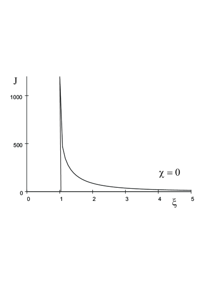
Figure 1: The plot of $J(\xi,0)$ which corresponds to the scattering on normal matter. All the tail lies in the retarded region $\xi>1$. Tails in the case $\chi\ll 1$ have similar form but contain an advanced part.

In the limit $\chi\rightarrow 0$ the distance between throats vanishes and the advanced signal is merely absent (e.g., in the region $0<\xi<1$ we get $J(\xi,0)=0$). All the scattered signal comes with a retarding. The infinite value of $J$ at $\xi=1$ does not mean that the echo is very strong, since it should be compared with the delta impulse (37). In considering the incident signal of a finite duration $\delta t$, the tail smoothes and takes a finite value. Indeed, for very small times $\xi-1\ll 1$ we have an approximation $\xi=1+\Delta\xi$ and therefore $J(\xi,0)=16\pi^{2}\left(\ln 2-\ln\Delta\xi+\frac{\Delta\xi}{2}\ln\frac{e\Delta\xi^{2}}{4}+...\right)$. Integrating this over $t^{\prime\prime}$ ($dt^{\prime\prime}=\Delta td\xi$, where $\Delta t=R/c$) gives already the finite value

$$<J(\xi=1,0)>=\frac{1}{\delta t}\int^{\delta t}_{0}J(\xi,0)dt^{\prime\prime}\simeq 16\pi^{2}(1+\ln\frac{2\Delta t}{\delta t}).$$ (47)

Qualitatively, the smoothed function $<J(\xi,0)>$ behaves as $J(\xi,\chi)$ for $\chi\ll 1$ which we describe below. The case $\chi=0$ corresponds to the scattering on normal matter when re-radiation has an isotropic character. In this case however the optical depth $\tau_{s}\ll 1$ and $\delta I_{\omega}/I_{\omega}^{0}\rightarrow 0$. We point out that the value $\tau_{s}$ has here the statistical character. In the case when there is an object, on the way of the ray, the echo signal may be considerable. This case is described by lensing or scattering on a single object.

Consider now the case of wormholes. For non-vanishing values $\chi$ the advanced signal does exist in the region $\xi>1-\chi$ and increases till the maximal value $J_{\max}$ which is reached at the point $\xi=1+\chi$. This gives

$$J_{\max}(\chi)=16\pi^{2}\left(\frac{\ln\left(\chi+1\right)}{\chi}-\frac{\ln\chi}{\left(\chi+1\right)}\right)\ .$$ (48)

The plot of $J_{max}$ is presented on Fig. 2.

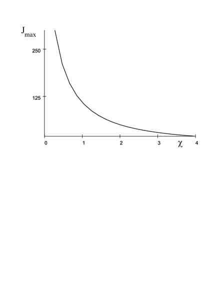
Figure 2: The plot of $J_{max}(\chi)=J(1+\chi,\chi)$. This function determines the maximal possible amplitude in echoes.

From (44) we see that $J_{max}$ determines the maximal possible amplitude in the echo. Different forms of tails $J(\xi,\chi)$ for different values of $\chi$ are presented on Fig. 3.

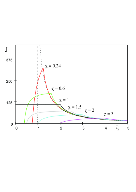
Figure 3: The form of tails $J(\xi,\chi)$ for a set of values of $\chi$. Advanced part of tails corresponds to $\xi<1$. For values $\chi>2$ tails possess only the retarded part.

Dashed line corresponds to the case $\chi\rightarrow 0$. The advanced signal corresponds to the region $\xi<1$ and it does exist only for values $\chi<2$. In the region $\chi>2$ the tail is completely retarded. In the approximation $\chi\gg 1$ we find

$$J(\xi,\chi)\simeq\frac{1}{\chi^{2}}J(\frac{\xi}{\chi},0)=\frac{8\pi^{2}}{\chi}\frac{2}{\xi}\ln\frac{\left(\xi+\chi\right)}{\left|\xi-\chi\right|}\theta\left(\xi-\chi\right).$$ (49)

Here the advanced signal is also absent (since the travel time to wormhole entrances exceeds the value $\Delta t=c/R$). As we see from Fig. 3 for sufficiently big $\xi$ the decrease of tails with time as $\sim 1/\xi\sim 1/t$ is the common feature of tails for all values of $\chi$.

VI.3 Structure of general GW signals with tails

In the case of a delta-like impulse the total signal is described by

$$I_{\omega}^{tot}\left(x,t\right)=\Phi_{\omega}^{0}\left[\delta\left(t-t^{\prime\prime}-\frac{R}{c}\right)+\frac{c}{R}\frac{\tau_{w}}{4\pi}J(\xi,\chi)\right],$$

where $\Phi_{\omega}^{0}$ is determined by (38). An arbitrary GW emission we obtain, if we replace $w_{0}(\omega)$ with a function $w_{0}(\omega,t^{\prime\prime})$ and integrate the above equation over $t^{\prime\prime}$. This defines the spectral energy flux as

$$I_{\omega}^{tot}=\frac{\omega^{2}}{c^{3}}\frac{w_{0}\left(\omega,t-\frac{R}{c}\right)}{R^{2}}+\int\frac{\omega^{2}}{c^{3}}\frac{w_{0}\left(\omega,t^{\prime\prime}\right)}{R^{2}}\frac{c}{R}\frac{\tau_{w}}{4\pi}J(\xi,\chi)dt^{\prime\prime}.$$

The typical duration of emission is very short, while the function $J(\xi,\chi)$ is very slow function (recall that $\xi=\frac{\left(t-t^{\prime\prime}-\eta\right)c}{R}$ almost does not change with a small change of $t^{\prime\prime}$, i.e., $\Delta\xi=c\Delta t^{\prime\prime}/R\ll 1$). This means that the multiplier $\frac{\tau_{w}}{4\pi}\frac{c}{R}J(\xi,\chi)$ can be taken at the moment of the start of emission $t^{\prime\prime}=t_{0}$ and can be removed from the integration. As it was pointed out above in the case $\chi=0$ one should replace $J$ with $<J>$ from (47) and for simplicity we set $\eta=0$. Then integrating this over frequencies $I=\int I_{\omega}d\omega$ we find

$$I(t)=I^{0}(t)+\frac{\tau_{w}}{4\pi}\frac{c}{R}J(\xi_{0},\chi)\int I^{0}(t)dt.$$ (50)

We see that tails have indeed a universal structure. For a short impulse $\int I^{0}dt\sim I^{0}\delta t\sim 2\pi I^{0}/\omega_{0}$, where $\delta t$ is the duration of the basic signal. The value $R/c=\Delta t$ is the propagation time, and therefore we find

$$\frac{\delta I}{I^{0}}\simeq\frac{\delta t}{\Delta t}\frac{\tau_{w}}{4\pi}J(\xi_{0},\chi)\ll 1.$$ (51)

The typical ratio $\frac{\delta t}{\Delta t}$ is extremely small $\frac{\delta t}{\Delta t}\sim 10^{-15}$ and, therefore, the direct detection of the tail signal is hardly possible. Indeed, the energy flux relates to the amplitude $h$ as follows

$$I=\frac{c^{3}}{32\pi G}\frac{1}{T}\int_{T}(\dot{h}_{\times}^{2}+\dot{h}_{+}^{2})dt,$$

where $h_{\times}$ and $h_{+}$ correspond to the two independent polarizations. Assuming the periodic signal $\sim e^{-i\omega_{0}t}$ we find

$$h^{2}+\delta h^{2}=\frac{16\pi G}{c^{3}\omega_{0}^{2}}I^{0}(t)\left(1+\frac{\delta I}{I^{0}}\right).$$

This explicitly shows that the tail contribution is $\delta h\ll h$. This means that the echo signals reported in Abedi, et al, (2017); Conklin, et al, (2018); Westerweck et al. (2018); Abedi & Afshordi (2019) cannot be explained as echoes from wormholes or ordinary compact objects. However, while the duration of the direct signal $h$ is very short, the tail part $\delta h^{2}$ decays with time very slowly $J(\xi_{0},\chi)\sim\Delta t/(\Delta t+t)\sim 1$ and the total energy in the tail, according to (43), may exceed the energy in the basic signal (i.e., $\int\delta h^{2}dt\gg\int h^{2}dt$). This means that the presence of such a heavy tail may be nevertheless observed by the increase of the noise level. The tails live for an extremely long period of time, at least $J(\xi_{0},\chi)\geq 1$ for $t\sim\Delta t$, and during this time all such tails from different binary merges accumulate. This roughly gives the additional multiplier $N\simeq\nu\Delta t$, where $\nu$ is the mean rate of events and this gives already the factor $\delta I/I^{0}\sim N\delta t\tau_{w}/(4\pi\Delta t)J(\xi_{0},\chi)\gtrsim 10^{-3}$ instead of (51), where we used for estimates $\nu\delta t\sim 10^{-5}$, $\chi=0.24$, and $\tau_{w}\sim 5$. Therefore the total noise level can be considerable and the reported in Abedi, et al, (2017); Conklin, et al, (2018); Westerweck et al. (2018); Abedi & Afshordi (2019) echoes may simply detect the stochastic background of GW radiation.

In conclusion we point out that we have assumed the specific model of the wormholes distribution when the distance between wormhole entrances has the same value $\Lambda=\left|\mathbf{R}_{+}-\mathbf{R}_{-}\right|$ and all wormholes have the same throat value $b=b_{0}$. To obtain the more general case we have to carry out an additional averaging with some probability density $p\left(\Lambda,b_{0}\right)$ which surely somewhat changes the structure of tails. This can be done directly in (50), (51).

VII Outlook

The topological bias for a distribution of wormholes can therefore be evaluated for Misner-Thorne wormhole by considering the neighborhood of each wormhole in the distribution after the modelizaition of the Dirac distribution for point-like sources after the characteristic sizes of the throats of each wormhole in the distribution, and by considering the related approximations for the $\beta$ function. Under this modellization, the emission of particles has to be expected within the same range of emission which can be considered not much far form the range of absorption.

The shift on the frequencies is estimated not higher than $10^{-3}$, so that it can be neglected. Such an estimate is very simple. First, peculiar velocities in galaxies (at edges) are around 300km/s, which gives $v/c\sim 10^{-3}$. This estimate works both for spirals and ellipticals. Second, there are peculiar velocities of clusters (observed by kinematic Sunyaev-Zel’dovich effect) which do not exceed $1500km/s$ which gives the Doppler shift $v/c\sim 5*10^{-3}$.

Rotation curves of spiral galaxies can be observed through several properties, such as Hubble type, structure, activity, and environment Sofue & Rubin (2001). A review on the literature about galaxy rotation curves can be found in Yegorova et al, (2012), while the possible observational errors are reviewed in Garcia et al, (2013). In Diaferio et al, (2005), the measurements of velocities of clusters due to kinematic Sunyaev-Zel’dovich effect are evaluated, for which the systematic errors are examined in Bhattacharya & Kosowsky (2008).

Thus the Doppler shift de Sousa (2010) expected does not exceed $0.5\%$, i.e. also at low frequencies Armstrong (2006). The experimental verification can be modelized at different astrophysical scales, Jain & Khoury (2010), i.e. also at satellite-distances scales Gerberding, et al (2015). In the analysis performed, throats have been assumed to participate in the peculiar motions.

For the local Universe ($z<0.1$) the shift due to the expansion can be estimated to be rather small as well (the frequency shift is less than $10\%$). For the more deep sources the dependence on the redshift can be easily incorporated, e.g., see discussions in Sec. VC. The most distant source GW170729 gives the shift of frequencies which does not exceed $30\%$. The behavior of a gravitational wave in several models of expanding universes was studied in Fabris & de Borba Goncalves (1998), while the behavior of a gravitational wave in an expanding Universe in the presence of a point-mass was schematized in Antoniou et al (2016).

Higher-order effects arising from Special Relativity and GR Will (1993); Maggiore (2007); Clifford & Will (2014) are discussed in Cooney et al. (2012) for comparison with constraints with more general metric theories of gravity and in Kayll (2004); Faber & Visser (2006) for comparison with constraints on dark-matter like contributions. We expect that higher-order corrections also do not essentially change the results presented.

In this manner we see that the Doppler shift of frequencies due to particular motions of wormholes can be neglected and the noise can be estimated to appear in the same frequency range as the original ingoing signal. The dependence on the redshift can not be so easily neglected or eliminated. The explicit form of the tails $J(\xi,\chi)$ corresponds to the local Universe when the redshift is neglected and for a particular distribution of wormholes having the same distance between entrances into every wormhole $\chi$. In a more general case we have to make some averaging over possible values of $\chi$. When the characteristic distance $\chi$ becomes very big the redshift becomes important. In particular, the most distant galaxy GN-z11 is observed at $z=11.09$ GN-z11 and we may expect that signals from binary merges may come even from more remote regions with $z>11$. In other words, together with the noise from the local Universe there should come a shifted noise from extremely remote regions. This problem however requires the further investigation.

VIII Acknowledgements

We acknowledge valuable comments and the advice of referees which helped us to clarify some important points and essentially improve the presentation of this work.

Appendix A Function $C(\chi)$

The function $C(\chi)$ is determined by the integral

$$C\left(\chi\right)\simeq\frac{1}{\left(4\pi\right)^{2}}\int\frac{d^{2}\Omega_{n}d^{2}\Omega_{l}}{\left|\chi\mathbf{n}+y\mathbf{l}-\mathbf{m}\right|^{2}}dy,$$

where $d^{2}\Omega$ is the solid angle. Assuming $\chi=\frac{\Lambda}{R}\ll 1$ we get $C(\chi)\approx C(0)$

$$\begin{array}[]{ll}C\left(0\right)=\frac{1}{2}\int_{0}^{\infty}\int_{0}^{\pi}\frac{d(\cos\theta)}{\left(y^{2}-2y\cos\theta+1\right)}dy=\\ =\frac{1}{2}\int_{0}^{\infty}\frac{1}{2y}\ln\frac{\left(y+1\right)^{2}}{\left(y-1\right)^{2}}dy=2.\,\allowbreak 4674.\end{array}$$ (52)

The opposite case $\chi\gg 1$ reduces to the analogous expression

$$C\left(\chi\right)\simeq\frac{1}{\chi}C\left(0\right).$$ (53)

In the general case we define $\mathbf{m}-\chi\mathbf{n}=\gamma\mathbf{k}$, where $\mathbf{k}^{2}=1$, $\gamma=\sqrt{\chi^{2}-2\chi\cos\alpha+1}$, and $\cos\alpha=(\mathbf{mn})$, then we get

$$C\left(\chi\right)=\frac{1}{\left(4\pi\right)^{2}}\int\left(\int\frac{d^{2}l}{\left|r\mathbf{l}-\mathbf{k}\right|^{2}}dr\right)\frac{d^{2}\Omega_{n}}{\gamma},$$

where $r=\frac{y}{\gamma}$. This transforms the integral into

$$\begin{array}[]{ll}C\left(\chi\right)\simeq\frac{1}{\left(4\pi\right)^{2}}\int\left(\frac{2\pi d(\cos\theta)}{\left(r^{2}-2r\cos\theta+1\right)}dr\right)\frac{d^{2}\Omega_{n}}{\gamma}=\frac{C\left(0\right)}{\left(4\pi\right)}\int\frac{d^{2}\Omega_{n}}{\gamma}\end{array}$$

which gives

$$C\left(\chi\right)=\frac{C\left(0\right)}{2}\int_{-1}^{1}\frac{d(\cos\alpha)}{\sqrt{\chi^{2}-2\chi\cos\alpha+1}}.$$

Finally we find the expression

$$\begin{array}[]{ll}C\left(\chi\right)=\frac{C\left(0\right)}{\left(2\chi\right)}\left(\left(\chi+1\right)-\left|\chi-1\right|\right)=\frac{C\left(0\right)}{\chi}\left\{\begin{array}[]{c}\chi,\ \ as\ \chi<1\\ 1,\ \ as\ \chi>1\end{array}\right..\end{array}$$ (54)

Appendix B Function $J(\xi,0)$

In the approximation $\chi\rightarrow 0$ eq. (45) reduces to

$$J(\xi,0)=\int\frac{\delta\left(\left|\mathbf{y}-\mathbf{m}\right|+y-\xi\right)}{\left|\mathbf{y}-\mathbf{m}\right|^{2}}\frac{d^{3}y}{y^{2}}d^{2}\Omega_{n}.$$ (55)

Let us use $x=\cos\theta$, then the above integral gives

$$J(\xi,0)=8\pi^{2}\int_{-1}^{1}\int_{0}^{\infty}\frac{\delta\left(y+\sqrt{y^{2}+2yx+1}-\xi\right)}{\left(y^{2}+2yx+1\right)}dydx.$$ (56)

Let us use new variable $u=\sqrt{y^{2}+2yx+1}>0$, $dx=\frac{u}{y}du$ whose range is $\left|y-1\right|<u<y+1$. Then we get

$$J(\xi,0)=8\pi^{2}\int_{0}^{\infty}\left(\int_{\left|y-1\right|}^{y+1}\delta\left(y+u-\xi\right)\frac{du}{u}\right)\frac{dy}{y}.$$ (57)

This integral splits in two parts which should be considered separately $J(\xi,0)=8\pi^{2}(J_{1}+J_{2})$

$$\begin{array}[]{ll}J_{1}=\int_{0}^{1}\left(\int_{1-y}^{1+y}\delta\left(y+u-\xi\right)\frac{du}{u}\right)\frac{dy}{y}\\ J_{2}=\int_{1}^{\infty}\left(\int_{y-1}^{y+1}\delta\left(y+u-\xi\right)\frac{du}{u}\right)\frac{dy}{y}.\end{array}$$

Consider the first part $J_{1}$. In the regions $\xi<1$ and $\xi>3$ the delta function has no roots and we find simply $J_{1}=0$. In the rest region $1<\xi<3$ the delta function possesses roots only for $y>\frac{1}{2}\left(\xi-1\right)$ and therefore

$$J_{1}=\int_{\frac{1}{2}\left(\xi-1\right)}^{1}\left(\int_{1-y}^{1+y}\delta\left(u-\left(\xi-y\right)\right)\frac{du}{u}\right)\frac{dy}{y},$$

which defines

$$J_{1}\left(\xi\right)=\int_{\frac{1}{2}\left(\xi-1\right)}^{1}\frac{dy}{\left(\xi-y\right)y}=\left\{\begin{array}[]{c}\allowbreak\frac{1}{\xi}\ln\frac{\left(\xi+1\right)}{\left(\xi-1\right)^{2}}\ as\ 1<\xi<3\\ 0\ \ as\ \xi\not\in[1,3]\end{array}\right..$$ (58)

Now let us consider the second part $J_{2}$. Again in the region $\xi<1$ the delta function has no roots and $J_{2}=0$. In the region $1<\xi<3$ roots exist for $y<\frac{1}{2}\left(\xi+1\right)$ and we find

$$J_{2}=\int_{1}^{\frac{1}{2}\left(\xi+1\right)}\frac{dy}{\left(\xi-y\right)y}=\frac{1}{\xi}\ln\left(\xi+1\right),\ as,\ 1<\xi<3\ .$$ (59)

In the region $\xi>3$ we find the upper and lower limits for $y$ as $y=\frac{1}{2}\left(\xi\pm 1\right)$ which gives

$$J_{2}=\int_{\frac{1}{2}\left(\xi-1\right)}^{\frac{1}{2}\left(\xi+1\right)}\frac{dy}{\left(\xi-y\right)y}=\frac{1}{\xi}\ln\frac{\left(\xi+1\right)^{2}}{\left(\xi-1\right)^{2}},\ as,\ \xi>3\ .$$ (60)

Now collecting all we find

$$J(\xi,0)=8\pi^{2}\frac{2}{\xi}\ln\frac{\left(\xi+1\right)}{\left(\xi-1\right)}\theta(\xi-1),$$ (61)

where $\theta(\xi-1)$ is the step function. We also point out that $\int J(\xi,0)d\xi=(4\pi)^{2}C(0)=8\pi^{2}\times 4.\,\allowbreak 9348$.

Appendix C Function $J(\xi,\chi)$

Consider the function $J(\xi,\chi)$ which is determined by the integral (45).

$$J(\xi,\chi)=\int\frac{\delta\left(\left|\mathbf{y}-\left(\mathbf{m-}\chi\mathbf{\mathbf{n}}\right)\right|+y-\xi\right)}{\left|\mathbf{y}-\left(\mathbf{m-}\chi\mathbf{\mathbf{n}}\right)\right|^{2}}\frac{d^{3}y}{y^{2}}d^{2}\Omega_{n}.$$

If we define new variables as $\mathbf{m}-\chi\mathbf{n}=\gamma\mathbf{k}$ with $\gamma=\sqrt{\chi^{2}-2\chi\cos\alpha+1}$, $\cos\alpha=(\mathbf{mn})$, and $r=y/\gamma$, then the integral reduces to the function $J(\xi,0)$ as

$$\begin{array}[]{ll}J(\xi,\chi)=\int\left(\int\frac{\delta\left(\left|\mathbf{r}-\mathbf{k}\right|+r-\frac{\xi}{\gamma}\right)}{\left|\mathbf{r}-\mathbf{k}\right|^{2}}\frac{d^{3}r}{r^{2}}\right)\frac{d^{2}\Omega_{n}}{\gamma^{2}}=\\ =\frac{1}{2}\int_{-1}^{1}J(\frac{\xi}{\gamma},0)\frac{d(\cos\alpha)}{\gamma^{2}}.\end{array}$$

Now by means of introducing $\gamma$ as a new integration variable instead of $\cos\alpha$ we find

$$J(\xi,\chi)=\frac{1}{2\chi}\int_{\left|\chi-1\right|}^{\chi+1}J(\frac{\xi}{\gamma},0)\frac{d\gamma}{\gamma}.$$ (62)

Substituting here (61) we get

$$J(\xi,\chi)=\frac{8\pi^{2}}{\chi}\int_{\frac{\left|\chi-1\right|}{\xi}}^{\frac{\chi+1}{\xi}}\ln\frac{\left(1+x\right)}{\left(1-x\right)}\theta\left(1-x\right)dx,$$ (63)

where $\theta\left(1-x\right)$ is the step function. This integral has different forms for different regions.

First region is $\xi<\left|\chi-1\right|$. It gives $x>1$ and, therefore,

$$J(\xi,\chi)=0,\ \ as\ \ \xi<\left|\chi-1\right|$$ (64)

The second region is $\left|\chi-1\right|<\xi<\chi+1$. The step function defines the upper limit $x=1$ and we get

$$\begin{array}[]{ll}J(\xi,\chi)=\frac{8\pi^{2}}{\chi}\left(\ln\left(\frac{4\xi^{2}}{\xi^{2}-\left(\chi-1\right)^{2}}\right)-\frac{\left|\chi-1\right|}{\xi}\ln\frac{\left(\xi+\left|\chi-1\right|\right)}{\left(\xi-\left|\chi-1\right|\right)}\right).\end{array}$$ (65)

The last region is $\xi>\chi+1$. Then $\theta\left(1-x\right)=1$ and we find

$$\begin{array}[]{ll}J=\frac{8\pi^{2}}{\chi}\left(\ln\frac{\xi^{2}-\left(\chi+1\right)^{2}}{\xi^{2}-\left(\chi-1\right)^{2}}+\frac{\chi+1}{\xi}\ln\frac{\left(\xi+\chi+1\right)}{\left(\xi-\chi-1\right)}-\frac{\left|\chi-1\right|}{\xi}\ln\frac{\left(\xi+\left|\chi-1\right|\right)}{\left(\xi-\left|\chi-1\right|\right)}\right).\end{array}$$ (66)

Appendix D Free motion

For a point-like source $\alpha_{k}=w_{0}\left(\omega\right)\delta\left(x-x^{\prime\prime}\right)\delta\left(t-t^{\prime\prime}\right)$ and in the absence of the scattering on wormholes (i.e., in the case of free motion) eq. (17) can be solved by the characteristics method. Indeed the geodesic motion of particles is described by rays

$$\mathbf{r}=\mathbf{r}_{0}+\mathbf{V}_{g}(t-t^{\prime\prime}),\ \mathbf{k}=\mathbf{k}_{0},\text{ }\mathbf{V}_{g}=\frac{\partial\omega}{\partial\mathbf{k}}=c\frac{\mathbf{k}}{k}.$$ (67)

Then, if we take $(k_{0},r_{0})$ as new coordinates, the energy density becomes $W\left[k\left(k_{0},r_{0},t\right),r\left(k_{0},r_{0},t\right)\right]=W\left(k_{0},r_{0},t\right)$ and (17) reads

$$\frac{dW\left(k_{0},r_{0},t\right)}{dt}=\alpha_{k}=w_{0}\left(\omega\right)\delta\left(\mathbf{r}_{0}-\mathbf{r}^{\prime\prime}\right)\delta\left(t-t^{\prime\prime}\right),$$ (68)

which has the obvious solution in the form

$$W\left(k_{0},r_{0},t\right)=w_{0}\left(\omega\right)\delta\left(\mathbf{r}_{0}-\mathbf{r}^{\prime\prime}\right)\theta\left(t-t^{\prime\prime}\right),$$ (69)

where $\theta\left(t-t^{\prime\prime}\right)$ is the step function ( $\theta\left(x\right)=1$ as $x>0$). Now to return to the initial coordinates $\left(k,r\right)$ we should simply replace back

$$\mathbf{r}_{0}=\mathbf{r}-\mathbf{V}_{g}(t-t^{\prime\prime}),\ \ \mathbf{k}_{0}=\mathbf{k},$$ (70)

which gives (we assume $t>t^{\prime\prime}$)

$$W_{k}\left(r,t\right)=w_{0}\left(\omega\right)\delta\left(\mathbf{r}-\mathbf{V}_{g}(t-t^{\prime\prime})-\mathbf{r}^{\prime\prime}\right).$$ (71)

In terms of the spherical coordinates $\mathbf{V}_{g}=(c,\theta^{\prime},\phi^{\prime})$ and $\mathbf{r}-\mathbf{r}^{\prime\prime}=\left(\left|\mathbf{r}-\mathbf{r}^{\prime\prime}\right|,\theta,\phi\right)$ the above expression transforms to

$$\begin{array}[]{cc}W_{k}(r,t)=\frac{w_{0}\left(\omega\right)}{c\left|\mathbf{r}-\mathbf{r}^{\prime\prime}\right|^{2}}\times\\ \times\delta\left(\frac{\left|\mathbf{r}-\mathbf{r}^{\prime\prime}\right|}{c}-t+t^{\prime\prime}\right)\delta\left(\cos\theta-\cos\theta^{\prime}\right)\delta\left(\phi-\phi^{\prime}\right).\end{array}$$

References

- Abbott, et al, (2016) Abbott B. P., et al., 2016, Phys. Rev. Lett. , 116, 061102
- Abbott, et al, (2017) Abbott B. P., et al. B. P., 2017, Astrophys. J., 851, L35, arXiv:1711.05578
- Kagra Collaboration (2019) Kagra Collaboration et al., 2019, Nature Astronomy, 3, 35
- Abedi, et al, (2017) Abedi J., Dykaar H. and Afshordi N., 2017, Phys. Rev. D, 96, 082004
- Conklin, et al, (2018) Conklin R. S., Holdom B. and Ren J., 2018, Phys. Rev. D, 98, 044021
- Westerweck et al. (2018) Westerweck J. et al., 2018, Phys. Rev. D, 97, 124037
- Abedi & Afshordi (2019) Abedi J. and Afshordi N., 2019, JCAP, 11, 010
- Cardoso, et al (2019) Cardoso V., et al., 2016, Phys. Rev. D, 94, 084031
- Cardoso & Pani (2019) Cardoso V. and Pani P., 2019, Living Rev. Rel., 22, 4
- Dai, et al (2018) Dai L., et al, 2018, Phys. Rev. D, 98, 104029
- Ambjorn et al. (2005) Ambjorn J., Jurkiewicz J., and Loll R. , 2005, Phys. Rev. Lett. , 95, 171301
- Laiho & Coumbe (2011) Laiho J. and Coumbe D., 2011, Phys. Rev. Lett. , 107, 161301,
- Clement (1984) Clement G., 1984, Int. J. Theor. Phys. 23, 335
- Kirillov & Savelova (2018) Kirillov A. A. & Savelova E. P., 2018, Universe, 4, 35
- Kirillov & Savelova (2008) Kirillov A. A. & Savelova E. P., 2008, Phys. Lett. B, 660, 93-99
- Kirillov & Savelova (2011) Kirillov A. A. & Savelova E. P., 2011, Mon. Not. RAS, 412, 1710
- Kirillov & Savelova (2020) Kirillov A. A. & Savelova E. P., 2020, Eur. Phys. J. C, 80:810
- Kang & Kim, (2018) Kang Y. and Kim S. W., 2018, J. Korean Phys. Soc. 73, 1800
- Kang & Kim (2019) Kang Y. and Kim S. W., 2019, The Gravitational Perturbation of a Morris-Thorne Wormhole and The Newman-Penrose Formalism, arXiv:1910.07715 [gr-qc].
- Morris & Thorne (1988) Morris M. S. and Thorne K. S., 1988, Am. J. Phys., 56, 395
- Fewster & Roman (2005) Fewster C. J. and Roman T. A., 2005, Phys. Rev. D, 72, 044023
- Ford & Roman (1995) Ford L. H. and Roman T. A., 1995, Phys. Rev. D, 51, 4277
- Ford & Roman (1996) Ford L. H. and Roman T. A., 1996, Phys. Rev. D, 53, 5496
- Kuhfittig (2009) Kuhfittig P. K. F., Theoretical construction of Morris-Thorne wormholes compatible with quantum field theory, arXiv:0908.4233 [gr-qc]
- Kim (2019) Kim H. C., Entropy of a Wormhole from the Constituent, arXiv:1911.00425 [gr-qc]
- Kim & Lee (2019) Kim H. C. and Lee Y., 2019, JCAP 1909 (2019) 001 doi:10.1088/1475-7516/2019/09/001
- Kim (2017) Kim H. C., 2017, Phys. Rev. D, 96, 064053
- Galvez et al. (2019) Galvez Ghersi J. T., Frolov A. V. and Dobre D. A., 2019, Class. Quant. Grav. 36, 135006
- Bueno et al. (2018) Bueno P., et al., 2018, Phys. Rev. D, 97, 024040
- Volkel & Kokkotas (2018) Volkel S. H. and Kokkotas K. D., 2018, Class. Quant. Grav., 35, 105018
- Visser (1989) Visser M., 1989, Traversable wormholes: Some simple examples, Phys. Rev. D, 39, 3182
- Shaikh et. al. (2019a) Shaikh R., et al., 2019, Phys. Lett. B, 789, 270
- Shaikh et. al. (2019b) Shaikh R., Banerjee P., Paul S. and Sarkar T., 2019, JCAP, 1907, 028
- Nandi et. al. (2017) Nandi K. K., et al., 2017, Phys. Rev. D, 95, 104011
- Yoo et. al. (2013) Yoo C. M., Harada T. and Tsukamoto N., 2013, Phys. Rev. D, 87, 084045
- Safonova et. al. (2002) Safonova M., Torres D. F., and Romero G. E., 2002, Phys. Rev. D, 65, 023001
- Bogdanov & Cherepashchuk (2008) Bogdanov M. and Cherepashchuk A., 2008, Astrophys. Space Sci. 317, 181
- Abe (2010) Abe F., 2010, Astrophys. J. 725, 787
- Kitamura et. al. (2011) Toki Y., Kitamura T., Asada H. and Abe F., 2011, Astrophys. J., 740, 121
- Kimet et. al. (2019) Kimet J., et al., Gravitational lensing by wormholes supported by electromagnetic, scalar, and quantum effects, 2019, European Physical Journal Plus, arXiv:1802.07680, DOI: 10.1140/epjp/i2019-12792-9
- Kim & Lee (2001) Kim S. W. and Lee H., 2001, Phys. Rev. D, 63, 064014
- Shaikh et al. (2019) Shaikh R., et al., 2019, Strong gravitational lensing by wormholes, arxiv 1905.06932, May 2019 Project: Gravitational lensing images and shadows as a probe of strong gravity.
- Geroch (1967) Geroch R. P., 1967, J. Math. Phys., 8, 782
- Kirillov & Savelova (2020) Kirillov A. A. & Savelova E. P., 2020, Eur. Phys. J. C, 80:45
- Kirillov & Savelova (2016) Kirillov A. A. & Savelova E. P., 2016, Int. Journ. Mod. Phys. D, 25, 1650075
- Bronnikov et al. (2013) Bronnikov K. A., Krechet V. G., and Lemos J. P. S., 2013, Phys. Rev. D, 87, 084060
- Bronnikov & Lemos (2009) Bronnikov K. A. & Lemos J. P. S., 2009, Phys. Rev. D, 79, 104019
- Bronnikov & Krechet (2019) Bronnikov K. A.& Krechet V. G., 2019, Phys. Rev. D, 99, 084051
- Bronnikov et al. (2019) Bronnikov K. A., Bolokhov S. V., and Skvortsova M. V., 2019, Int. J. Mod. Phys. D 28, 1941008
- Hochberg et al. (1997) Hochberg D., Popov A., Sushkov S. V., 1997, Phys. Rev. Lett. , 78, 2050
- Hochberg et al. (2013) Harko T., Lobo F. S. N., Mak M. K., Sushkov S. V., 2013, Phys. Rev. D, D87, 067504
- Myrzakulov et al. (2016) Myrzakulov R., Sebastiani L., Vagnozzi S., Zerbini S., 2016, Class. Quant. Gravit. 33, 125005
- Kirillov et al, (2008) Kirillov A. A., Savelova E. P., Zolotarev P. S., 2008, Phys. Lett. B 663, 372
- Culter & Flanagan (1997) Culter C. and Flanagan E. E., 1997, Phys. Rev. D, 49, 2658
- Sofue & Rubin (2001) Sofue Y. and Rubin V., 2001, Ann. Rev. Astron. Astrophys. 39, 137
- Yegorova et al, (2012) Yegorova I. A., Babic A., Salucci P., Spekkens K. and Pizzella A., 2012, Astron. Astrophys. Trans. 27, 335
- Garcia et al, (2013) Garcia R. A., Ceillier T., Mathur S. and Salabert D., 2013, ASP Conf. Ser. 479, 129
- Diaferio et al, (2005) Diaferio A., et al., 2005, Mon. Not. Roy. Astron. Soc., 356, 1477
- Bhattacharya & Kosowsky (2008) Bhattacharya S. and Kosowsky A., 2008, JCAP 0808, 030
- de Sousa (2010) de Sousa C. M. G., 2010, Mod. Phys. Lett. A 25, 1455
- Armstrong (2006) Armstrong J., 2006, Living Rev. Relativity, 9, 1
- Jain & Khoury (2010) Jain B. and Khoury J., 2010, Annals Phys. 325, 1479
- Gerberding, et al (2015) Gerberding O., et al., 2015, Rev. Sci. Instrum. 86, 074501
- Fabris & de Borba Goncalves (1998) Fabris J. C. and de Borba Goncalves S. V., 1998, Gravitational waves in an expanding universe, gr-qc/9808007.
- Antoniou et al (2016) Antoniou I., Papadopoulos D. and Perivolaropoulos L., 2016, Phys. Rev. D, 94, 084018
- Will (1993) Will C. M., Theory and Experiment in Gravitational Physics, CUP 1993, New York.
- Maggiore (2007) Maggiore Michele, 2007, Gravitational Waves Volume 1: Theory and Experiments, OUP UK 2007
- Clifford & Will (2014) Clifford M., Will C. M., Living Rev. Relativ. 2014 17: 4
- Cooney et al. (2012) Cooney A., Psaltis D. and Zaritsky D., Special and General Relativistic Effects in Galactic Rotation Curves, arXiv:1202.2853 [astro-ph.GA].
- Kayll (2004) Kayll L., 2004, Phys. Rev. Lett. , 92, 051101
- Faber & Visser (2006) Faber T. and Visser M., 2006, Mon. Not. Roy. Astron. Soc., 372, 136
- (72) Oesch, P. A. et al., 2016, Astrophys. J. 819, 129