Testing Conditional Independence via
Quantile Regression Based Partial Copulas

Abstract

The partial copula provides a method for describing the dependence between two random variables $X$ and $Y$ conditional on a third random vector $Z$ in terms of nonparametric residuals $U_{1}$ and $U_{2}$. This paper develops a nonparametric test for conditional independence by combining the partial copula with a quantile regression based method for estimating the nonparametric residuals. We consider a test statistic based on generalized correlation between $U_{1}$ and $U_{2}$ and derive its large sample properties under consistency assumptions on the quantile regression procedure. We demonstrate through a simulation study that the resulting test is sound under complicated data generating distributions. Moreover, in the examples considered the test is competitive to other state-of-the-art conditional independence tests in terms of level and power, and it has superior power in cases with conditional variance heterogeneity of $X$ and $Y$ given $Z$.

Keywords: Conditional independence testing, nonparametric testing, partial copula, conditional distribution function, quantile regression

1 Introduction

This paper introduces a new class of nonparametric tests of conditional independence between real-valued random variables, $X\mathrel{\text{\scalebox{1.07}{$\perp\mkern-10.0mu\perp$}}}Y\mid Z$, based on quantile regression. Conditional independence is an important concept in many statistical fields such an graphical models and causal inference (Lauritzen, 1996; Spirtes et al., 2000; Pearl, 2009). However, Shah and Peters (2020) proved that conditional independence is an untestable hypothesis when the distribution of $(X,Y,Z)$ is only assumed to be absolutely continuous with respect to Lebesgue measure.

More precisely, let $\mathcal{P}$ denote the set of distributions of $(X,Y,Z)$ that are absolutely continuous with respect to Lebesgue measure. Let $\mathcal{H}\subset\mathcal{P}$ be those distributions for which conditional independence holds. Then Shah and Peters (2020) showed that if $\psi_{n}$ is a hypothesis test for conditional independence with uniformly valid level $\alpha\in(0,1)$ over $\mathcal{H}$,

$$\sup_{P\in\mathcal{H}}E_{P}(\psi_{n})\leq\alpha,$$

then the test cannot have power greater than $\alpha$ against any alternative $P\in\mathcal{Q}:=\mathcal{P}\setminus\mathcal{H}$. This is true even when restricting the distribution of $(X,Y,Z)$ to have bounded support. The purpose of this paper is to identify a subset $\mathcal{P}_{0}\subset\mathcal{P}$ of distributions and a test $\psi_{n}$ that has asymptotic (uniform) level over $\mathcal{P}_{0}\cap\mathcal{H}$ and power against a large set of alternatives within $\mathcal{P}_{0}\backslash\mathcal{H}$.

Our starting point is the so-called partial copula construction. Letting $F_{X\mid Z}$ and $F_{Y\mid Z}$ denote the conditional distribution functions of $X$ given $Z$ and $Y$ given $Z$, respectively, we define random variables $U_{1}$ and $U_{2}$ by

$$U_{1}:=F_{X\mid Z}(X\mid Z)\quad\text{and}\quad U_{2}:=F_{Y\mid Z}(Y\mid Z).$$

Then the joint distribution of $U_{1}$ and $U_{2}$ is called the partial copula and it can be shown that $X\mathrel{\text{\scalebox{1.07}{$\perp\mkern-10.0mu\perp$}}}Y\mid Z$ implies $U_{1}\mathrel{\text{\scalebox{1.07}{$\perp\mkern-10.0mu\perp$}}}U_{2}$. Thus the question about conditional independence can be transformed into a question about independence. The main challenge with this approach is that the conditional distribution functions are unknown and must be estimated.

In Section 3 we propose an estimator of conditional distribution functions based on quantile regression. More specifically, we let $\mathcal{T}=[\tau_{\min},\tau_{\max}]$ be a range of quantile levels for $0<\tau_{\min}<\tau_{\max}<1$, and let $Q(\mathcal{T}\mid z)$ denote the range of conditional $\mathcal{T}$-quantiles in the distribution $X\mid Z=z$. To estimate a conditional distribution function $F$ given a sample $(X_{i},Z_{i})_{i=1}^{n}$ we propose to perform quantile regressions $\hat{q}_{k,z}=\hat{Q}^{(n)}(\tau_{k}\mid z)$ along an equidistant grid of quantile levels $(\tau_{k})_{k=1}^{m}$ in $\mathcal{T}$, and then construct the estimator $\hat{F}^{(m,n)}$ by linear interpolation of the points $(\hat{q}_{k,z},\tau_{k})_{k=1}^{m}$. The main result of the first part of the paper is Theorem 5, which states that we can achieve the following bound on the estimation error

$$\|F-\hat{F}^{(m,n)}\|_{\mathcal{T},\infty}:=\sup_{z}\sup_{t\in Q(\mathcal{T}\mid z)}|F(t\mid z)-\hat{F}^{(m,n)}(t\mid z)|\in\mathcal{O}_{P}(g_{P}(n))$$

where $g_{P}$ is a rate function describing the $\mathcal{O}_{P}$-consistency of the quantile regression procedure over the conditional $\mathcal{T}$-quantiles for $P$ in a specified set of distributions $\mathcal{P}_{0}\subset\mathcal{P}$. This result demonstrates how pointwise consistency of a quantile regression procedure over $\mathcal{P}_{0}$ can be transferred to the estimator $\hat{F}^{(m,n)}$, and we discuss how this can be extended to uniform consistency over $\mathcal{P}_{0}$. We conclude the section by reviewing a flexible model class from quantile regression where such consistency results are available.

In Section 4 we describe a generic method for testing conditional independence based on estimated conditional distribution functions, $\hat{F}_{X\mid Z}^{(n)}$ and $\hat{F}^{(n)}_{Y\mid Z}$, obtained from a sample $(X_{i},Y_{i},Z_{i})_{i=1}^{n}$. From these estimates we compute

$$\hat{U}_{1,i}^{(n)}:=\hat{F}^{(n)}_{X\mid Z}(X_{i}\mid Z_{i})\quad\text{and}\quad\hat{U}_{2,i}^{(n)}:=\hat{F}^{(n)}_{Y\mid Z}(Y_{i}\mid Z_{i}),$$

for $i=1,\dots,n$, which can then be plugged into a bivariate independence test. If $\hat{F}_{X\mid Z}^{(n)}$ and $\hat{F}^{(n)}_{Y\mid Z}$ are consistent with a sufficiently fast rate of convergence, properties of the bivariate test, in terms of level and power, can be transferred to the test of conditional independence. The details of this transfer of properties depend on the specific test statistic. The main contribution of the second part of the paper is a detailed treatment of a test given in terms of a generalized correlation, estimated as

$$\hat{\rho}_{n}:=\frac{1}{n}\sum_{i=1}^{n}\varphi\left(\hat{U}_{1,i}^{(n)}\right)\varphi\left(\hat{U}_{2,i}^{(n)}\right)^{T}$$

for a function $\varphi=(\varphi_{1},\dots,\varphi_{q}):[0,1]\to\mathbb{R}^{q}$ satisfying certain regularity conditions. A main result is Theorem 14, which states that $\sqrt{n}\hat{\rho}_{n}$ converges in distribution toward $\mathcal{N}(0,\Sigma\otimes\Sigma)$ under the hypothesis of conditional independence whenever $\hat{F}_{X\mid Z}^{(n)}$ and $\hat{F}^{(n)}_{Y\mid Z}$ are $\mathcal{O}_{P}$-consistent with rates $g_{P}$ and $h_{P}$ satisfying $\sqrt{n}g_{P}(n)h_{P}(n)\to 0$. The covariance matrix $\Sigma$ depends only on $\varphi$. We use this to show asymptotic pointwise level of the test when restricting to the set of distributions $\mathcal{P}_{0}$ where the required consistency can be obtained. We then proceed to show in Theorem 18 that $\sqrt{n}\hat{\rho}_{n}$ diverges in probability under a set of alternatives of conditional dependence when we have $\mathcal{O}_{P}$-consistency of the conditional distribution function estimators. This we use to show asymptotic pointwise power of the test. We also show how asymptotic uniform level and power can be achieved when $\hat{F}_{X\mid Z}^{(n)}$ and $\hat{F}^{(n)}_{Y\mid Z}$ are uniformly consistent over $\mathcal{P}_{0}$. Lastly, we provide an out-of-the-box procedure for conditional independence testing in conjunction with our quantile regression based conditional distribution function estimator $\hat{F}^{(m,n)}$ from Section 3.

In Section 5 we examine the proposed test through a simulation study where we assess the level and power properties of the test and benchmark it against existing nonparametric conditional independence tests. All proofs are collected in Appendix A.

2 Related Work

The partial copula and its application for conditional independence testing was initially introduced by Bergsma (2004) and further explored by Bergsma (2011). Its use for conditional independence testing has also been explored by Song (2009), Patra et al. (2016) and Liu et al. (2018). Moreover, properties of the partial copula was studied by Gijbels et al. (2015) and Spanhel and Kurz (2016) among others. A related but different approach for testing conditional independence via the factorization of the joint copula of $(X,Y,Z)$ is given by Bouezmarni et al. (2012). Common for the existing approaches to using the partial copula for conditional independence testing is that the conditional distribution functions $F_{X\mid Z}$ and $F_{Y\mid Z}$ are estimated using a kernel smoothing procedure (Stute et al., 1986; Einmahl and Mason, 2005). The advantage of the approach is that the estimator is nonparametric, however, it does not scale well with the dimension of the conditioning variable $Z$. This is partly remedied by Haff and Segers (2015) who suggest a nonparametric pair-copula estimator whose convergence rate is independent of the dimension of $Z$. This estimator requires the simplifying assumption, which is a strong assumption not required for the validity of our approach. Moreover, it is not obvious how to incorporate parametric assumptions, such as a certain functional dependence between response and covariates, using kernel smoothing estimators, since there is only the choice of a kernel and a bandwidth. Furthermore, a treatment of the relationship between level and power properties of a partial copula based conditional independence test, and consistency of the conditional distribution function estimator is lacking in the existing literature. In this work we take a novel approach to testing conditional independence using the partial copula by using quantile regression for estimating the conditional distribution functions. This allows for a distribution free modeling of the conditional distributions $X\mid Z=z$ and $Y\mid Z=z$ that can handle high-dimensionality of $Z$ through penalization, and complicated response-predictor relationships by basis expansions. We also make the requirements on consistency of the conditional distribution function estimator that are needed to obtain level and power of the test explicit. A similar recent approach to testing conditional independence using regression methods is given by Shah and Peters (2020), who propose to test for vanishing correlation between the residuals after nonparametric conditional mean regression of $X$ on $Z$ and $Y$ on $Z$. See also Ramsey (2014) and Fan et al. (2020). This approach captures dependence between $X$ and $Y$ given $Z$ that lies in the conditional correlation. However, as is demonstrated through a simulation study in Section 5.5, it does not adequately account for conditional variance heterogeneity between $X$ and $Y$ given $Z$, while our partial copula based test captures the dependence more efficiently.

3 Estimation of Conditional Distribution Functions

Throughout the paper we restrict ourselves to the set of distributions $\mathcal{P}$ over the hypercube $[0,1]^{2+d}$ that are absolutely continuous with respect to Lebesgue measure. Let $(X,Y,Z)\sim P\in\mathcal{P}$ such that $X,Y\in[0,1]$ and $Z\in[0,1]^{d}$. When we speak of the distribution of $X$ given $Z$ relative to $P$ we mean the conditional distribution that is induced when $(X,Y,Z)\sim P$. In this section we consider estimation of the conditional distribution function $F_{X\mid Z}$ of $X$ given $Z$ using quantile regression. Estimation of $F_{Y\mid Z}$ can be carried out analogously.

3.1 Conditional distribution and quantile functions

Given $z\in[0,1]^{d}$ we denote by

$$F_{X\mid Z}(t\mid z):=P(X\leq t\mid Z=z)$$

the conditional distribution function of $X\mid Z=z$ for $t\in[0,1]$. We denote by

$$Q_{X\mid Z}(\tau\mid z):=\inf\{t\in[0,1]\mid F_{X\mid Z}(t\mid z)\geq\tau\}$$

the conditional quantile function of the conditional distribution $X\mid Z=z$ for $\tau\in[0,1]$ and $z\in[0,1]^{d}$. We will omit the subscript in $F_{X\mid Z}$ and $Q_{X\mid Z}$ when the conditional distribution of interest is clear from the context.

In quantile regression one models the function $z\mapsto Q(\tau\mid z)$ for fixed $\tau\in[0,1]$. Estimation of the quantile regression function is carried out by solving the empirical risk minimization problem

$$\hat{Q}(\tau\mid\cdot)\in\operatorname*{arg\,min}_{f\in\mathcal{F}}\sum_{i=1}^{n}L_{\tau}\left(X_{i}-f(Z_{i})\right)$$

where the loss function $L_{\tau}(u)=u(\tau-1(u<0))$ is the so-called check function and $\mathcal{F}$ is some function class. For $\tau=1/2$ the loss function is $L_{1/2}(u)=|u|$, and we recover median regression as a special case. One can also choose to add regularization as with conditional mean regression. See Koenker (2005) and Koenker et al. (2017) for an overview of the field.

3.2 Quantile regression based estimator

Based on the conditional quantile function $Q$ we define an approximation $\tilde{F}^{(m)}$ of the conditional distribution function $F$ as follows. We let $\tau_{\min}$ and $\tau_{\max}$ denote fixed quantile levels satisfying $0<\tau_{\min}<\tau_{\max}<1$, and we let $q_{\min,z}:=Q(\tau_{\min}\mid z)>0$ and $q_{\max,z}:=Q(\tau_{\max}\mid z)<1$ denote the corresponding conditional quantiles.

Let $\mathcal{T}=[\tau_{\min},\tau_{\max}]$ denote the set of potential quantile levels. A grid in $\mathcal{T}$ is a sequence $(\tau_{k})_{k=1}^{m}$ such that $\tau_{\min}=\tau_{1}<\cdots<\tau_{m}=\tau_{\max}$ for $m\geq 2$. An equidistant grid is a grid $(\tau_{k})_{k=1}^{m}$ for which $\tau_{k+1}-\tau_{k}$ is constant for $k=1,\dots,m-1$. Also let $\tau_{0}=0$ and $\tau_{m+1}=1$ be fixed.

Given a grid $(\tau_{k})_{k=1}^{m}$ we let $q_{k,z}:=Q(\tau_{k}\mid z)$ for $k=1,\dots,m$ and define $q_{0,z}:=0$ and $q_{m+1,z}:=1$. For each $z\in[0,1]^{d}$ we define a function $\tilde{F}^{(m)}(\cdot\mid z):[0,1]\to[0,1]$ by linear interpolation of the points $(q_{k,z},\tau_{k})_{k=0}^{m+1}$:

$$\tilde{F}^{(m)}(t\mid z):=\sum_{k=0}^{m}\left(\tau_{k}+(\tau_{k+1}-\tau_{k})\frac{t-q_{k,z}}{q_{k+1,z}-q_{k,z}}\right)1_{(q_{k,z},q_{k+1,z}]}(t).$$ (1)

Let $Q(\mathcal{T}\mid z)=[q_{\min,z},q_{\max,z}]$ be the range of conditional $\mathcal{T}$-quantiles in the conditional distribution $X\mid Z=z$ for $z\in[0,1]^{d}$, and define the supremum norm

$$\|f\|_{\mathcal{T},\infty}=\sup_{z\in[0,1]^{d}}\sup_{t\in Q(\mathcal{T}\mid z)}|f(t,z)|$$

for a function $f:[0,1]\times[0,1]^{d}\to\mathbb{R}$. Note that this is a norm on the set of bounded functions on $\{(t,z)\mid z\in[0,1]^{d},t\in Q(\mathcal{T}\mid z)\}$. Then we have the following approximation result.

Proposition 1

Denote by $\tilde{F}^{(m)}$ the function (1) defined from a grid $(\tau_{k})_{k=1}^{m}$ in $\mathcal{T}$. Then it holds that

$$||F-\tilde{F}^{(m)}||_{\mathcal{T},\infty}\leq\kappa_{m}$$

where $\kappa_{m}:=\max_{k=1,\dots,m-1}(\tau_{k+1}-\tau_{k})$ is the coarseness of the grid.

Choosing a finer and finer grid yields $\kappa_{m}\to 0$, which implies that $\tilde{F}^{(m)}\to F$ in the norm $\|\cdot\|_{\mathcal{T},\infty}$ for $m\to\infty$.

By an estimator of the conditional distribution function $F$ we mean a mapping from a sample $(X_{i},Z_{i})_{i=1}^{n}$ to a function $\hat{F}^{(n)}(\cdot\mid z):[0,1]\to[0,1]$ such that for every $z\in[0,1]^{d}$ it holds that $t\mapsto\hat{F}^{(n)}(t\mid z)$ is continuous and increasing with

$$\hat{F}^{(n)}(0\mid z)=0\quad\text{and}\quad\hat{F}^{(n)}(1\mid z)=1.$$

Motivated by (1) we define the following estimator of the conditional distribution function.

Definition 2

Let $(\tau_{k})_{k=1}^{m}$ be a grid in $\mathcal{T}$. Define $\hat{q}^{(n)}_{0,z}:=0$ and $\hat{q}_{m+1,z}^{(n)}:=1$, and let $\hat{q}^{(n)}_{k,z}:=\hat{Q}^{(n)}(\tau_{k}\mid z)$ for $k=1,\dots,m$ be the predictions of a quantile regression model obtained from an i.i.d. sample $(X_{i},Z_{i})_{i=1}^{n}$. We define the estimator $\hat{F}^{(m,n)}(\cdot\mid z):[0,1]\to[0,1]$ by

$$\hat{F}^{(m,n)}(t\mid z):=\sum_{k=0}^{m}\left(\tau_{k}+(\tau_{k+1}-\tau_{k})\frac{t-\hat{q}^{(n)}_{k,z}}{\hat{q}^{(n)}_{k+1,z}-\hat{q}^{(n)}_{k,z}}\right)1_{\left(\hat{q}^{(n)}_{k,z},\hat{q}^{(n)}_{k+1,z}\right]}(t)$$ (2)

for each $z\in[0,1]^{d}$.

Note that the estimator is not monotone in the presence of quantile crossing (He, 1997). In this case we perform a re-arrangement of the estimated conditional quantiles in order to obtain monotonicity for finite sample size (Chernozhukov et al., 2010). However, the estimated conditional quantiles will be ordered correctly under the consistency assumptions that we will introduce in Assumption 1, that is, the re-arrangement becomes unnecessary, and the estimator becomes monotone with high probability as $n\to\infty$ for any grid $(\tau_{k})_{k=1}^{m}$ in $\mathcal{T}$.

3.3 Pointwise consistency of $\hat{F}^{(m,n)}$

We will now demonstrate how pointwise consistency of the proposed estimator over a set of distributions $\mathcal{P}_{0}\subset\mathcal{P}$ can be obtained under the assumption that the quantile regression procedure is pointwise consistent over $\mathcal{P}_{0}$.

We will evaluate the consistency of $\hat{F}^{(m,n)}$ according to the supremum norm $||\cdot||_{\mathcal{T},\infty}$ introduced in Section 3.2, that is, we restrict the supremum to be over $t\in Q(\mathcal{T}\mid z)$ and not the entire interval $[0,1]$. We do so because quantile regression generally does not give uniform consistency of all extreme quantiles, and in Section 4 we show how consistency of $\hat{F}^{(m,n)}$ between the conditional $\tau_{\min}$- and $\tau_{\max}$-quantiles is sufficient for conditional independence testing.

First, we have the following key corollary of Proposition 1, which is a simple application of the triangle inequality.

Corollary 3

Let $\tilde{F}^{(m)}$ and $\hat{F}^{(m,n)}$ be given by (1) and (2), respectively. Then

$$\|F-\hat{F}^{(m,n)}\|_{\mathcal{T},\infty}\leq\kappa_{m}+\|\tilde{F}^{(m)}-\hat{F}^{(m,n)}\|_{\mathcal{T},\infty}$$

for all grids $(\tau_{k})_{k=1}^{m}$ in $\mathcal{T}$.

The random part of the right hand side of the inequality is the term $\|\tilde{F}^{(m)}-\hat{F}^{(m,n)}\|_{\mathcal{T},\infty}$, while $\kappa_{m}$ is deterministic and only depends on the choice of grid $(\tau_{k})_{k=1}^{m}$. Controlling the term $\|\tilde{F}^{(m)}-\hat{F}^{(m,n)}\|_{\mathcal{T},\infty}$ is an easier task than controlling $\|F-\hat{F}^{(m,n)}\|_{\mathcal{T},\infty}$ directly because $\tilde{F}^{(m)}$ and $\hat{F}^{(m,n)}$ are piecewise linear, while $F$ is only assumed to be continuous and increasing.

Consistency assumptions on the quantile regression procedure will allow us to show consistency of the estimator $\hat{F}^{(m,n)}$. Let the random variable

$$\mathcal{D}_{\mathcal{T}}^{(n)}:=\sup_{z\in[0,1]^{d}}\sup_{\tau\in\mathcal{T}}|Q(\tau\mid z)-\hat{Q}^{(n)}(\tau\mid z)|$$

denote the uniform prediction error of a fitted quantile regression model, $\hat{Q}^{(n)}$, over the set of quantile levels $\mathcal{T}=[\tau_{\min},\tau_{\max}]$. Below we write $X_{n}\in\mathcal{O}_{P}(a_{n})$ when $X_{n}$ is big-O in probability of $a_{n}$ with respect to $P$. See Appendix B for the formal definition.

Assumption 1

For each $P\in\mathcal{P}_{0}$ there exist

• a deterministic rate function $g_{P}$ tending to zero as $n\to\infty$ such that $\mathcal{D}_{\mathcal{T}}^{(n)}\in\mathcal{O}_{P}(g_{P}(n))$

• and a finite constant $C_{P}$ such that the conditional density $f_{X\mid Z}$ satisfies

  $$\sup_{x\in[0,1]}f_{X\mid Z}(x\mid z)\leq C_{P}$$

  for almost all $z\in[0,1]^{d}.$

Assumption 1 (i) is clearly necessary to achieve consistency of the estimator. Assumption 1 (ii) is a regularity condition that is used to ensure that $q_{k+1,z}-q_{k,z}$ does not tend to zero too fast as $\kappa_{m}\to 0$. We now have:

Proposition 4

Let Assumption 1 be satisfied. Then

$$\|\tilde{F}^{(m)}-\hat{F}^{(m,n)}\|_{\mathcal{T},\infty}\in\mathcal{O}_{P}(g_{P}(n))$$

for each fixed $P\in\mathcal{P}_{0}$ and all equidistant grids $(\tau_{k})_{k=1}^{m}$ in $\mathcal{T}$.

Consider letting the number of grid points $m_{n}$ depend on the sample size $n$. By combining Corollary 3 and Proposition 4 we obtain the main pointwise consistency result.

Theorem 5

Let Assumption 1 be satisfied. Then

$$\|F-\hat{F}^{(m_{n},n)}\|_{\mathcal{T},\infty}\in\mathcal{O}_{P}(g_{P}(n))$$

for each fixed $P\in\mathcal{P}_{0}$ given that the equidistant grids $(\tau_{k})_{k=1}^{m_{n}}$ in $\mathcal{T}$ satisfy $\kappa_{m_{n}}\in o(g_{P}(n))$.

This shows that $\hat{F}^{(m_{n},n)}$ is pointwise consistent over $\mathcal{P}_{0}$ given that the quantile regression procedure is pointwise consistent over $\mathcal{P}_{0}$. Moreover, we can transfer the rate of convergence $g_{P}$ directly. In Section 4.4 we will use this type of pointwise consistency to show asymptotic pointwise level and power of our conditional independence test over $\mathcal{P}_{0}$.

Note that we can estimate conditional distribution functions in settings with high dimensional covariates to the extend that the quantile regression estimation procedure can deal with high dimensionality. An example of such a procedure is given in Section 3.5.

We chose to state Proposition 4 and Theorem 5 for equidistant grids only, but in the proof of Proposition 4 we only need that the ratio $\kappa_{m}/\gamma_{m}$ between the coarseness $\kappa_{m}$ and the smallest subinterval $\gamma_{m}=\min_{k=1,\dots,m-1}(\tau_{k+1}-\tau_{k})$ must not diverge as $m\to\infty$. This is obviously ensured for an equidistant grid. Moreover, for an equidistant grid, $\kappa_{m}=(\tau_{\max}-\tau_{\min})/(m-1)$, and $\kappa_{m_{n}}\in o(g_{P}(n))$ if $m_{n}$ grows with rate at least $g_{P}(n)^{-(1+\varepsilon)}$ for some $\varepsilon>0$. Since the rate is unknown in practical applications we choose $m$ to be the smallest integer larger than $\sqrt{n}$ as a rule of thumb, since this represents the optimal parametric rate.

3.4 Uniform consistency of $\hat{F}^{(m,n)}$

The pointwise consistency result of Theorem 5 can be extended to a uniform consistency over $\mathcal{P}_{0}$ by strengthening Assumption 1 to hold uniformly. Below we write $X_{n}\in\mathcal{O}_{\mathcal{M}}(a_{n})$ when $X_{n}$ is big-O in probability of $a_{n}$ uniformly over a set of distributions $\mathcal{M}$. We refer to Appendix B for the formal definition.

Assumption 2

For $\mathcal{P}_{0}\subset\mathcal{P}$ there exist

• a deterministic rate function $g$ tending to zero as $n\to\infty$ such that $\mathcal{D}_{\mathcal{T}}^{(n)}\in\mathcal{O}_{\mathcal{P}_{0}}(g(n))$

• and a finite constant $C$ such that the conditional density $f_{X\mid Z}$ satisfies

  $$\sup_{x\in[0,1]}f_{X\mid Z}(x\mid z)\leq C$$

  for almost all $z\in[0,1]^{d}$.

With this stronger assumption we have a uniform extension of Proposition 4.

Proposition 6

Let Assumption 2 be satisfied. Then

$$\|\tilde{F}^{(m)}-\hat{F}^{(m,n)}\|_{\mathcal{T},\infty}\in\mathcal{O}_{\mathcal{P}_{0}}(g(n)).$$

for all equidistant grids $(\tau_{k})_{k=1}^{m}$ in $\mathcal{T}$.

We can now combine Corollary 3 with the stronger Proposition 6 to obtain the following uniform consistency of the estimator $\hat{F}^{(m,n)}$.

Theorem 7

Suppose that Assumption 2 is satisfied. Then

$$\|{F}-\hat{F}^{(m_{n},n)}\|_{\mathcal{T},\infty}\in\mathcal{O}_{\mathcal{P}_{0}}(g(n))$$

given that the equidistant grids $(\tau_{k})_{k=1}^{m_{n}}$ in $\mathcal{T}$ satisfy $\kappa_{m_{n}}\in o(g(n))$.

This shows that our estimator $\hat{F}^{(m,n)}$ can achieve uniform consistency over a set of distributions $\mathcal{P}_{0}\subset\mathcal{P}$ given that the quantile regression procedure is uniformly consistent over $\mathcal{P}_{0}$. In Section 4.5 we show how this strenghtened result can be used to establish asymptotic uniform level and power of our conditional independence test over $\mathcal{P}_{0}$.

3.5 A quantile regression model

In this section we will provide an example of a flexible quantile regression model and estimation procedure where consistency results are available. Consider the model

$$Q(\tau\mid z)=h(z)^{T}\beta_{\tau}$$ (3)

where $h:[0,1]^{d}\to\mathbb{R}^{p}$ is a known and continuous transformation of $Z$, e.g., a polynomial or spline basis expansion to model non-linear effects. Inference in the model (3) was analyzed by Belloni and Chernozhukov (2011) and Belloni et al. (2019) in the high-dimensional setup $p\gg n$. In the following we describe a subset of their results that is relevant for our application. Given an i.i.d. sample $(X_{i},Z_{i})_{i=1}^{n}$ and a fixed quantile regression level $\tau\in(0,1)$, estimation of $\beta_{\tau}\in\mathbb{R}^{p}$ is carried out by penalized regression:

$$\hat{\beta}_{\tau}\in\operatorname*{arg\,min}_{\beta\in\mathbb{R}^{p}}\sum_{i=1}^{n}L_{\tau}(X_{i}-h(Z_{i})^{T}\beta)+\lambda_{\tau}\|\beta\|_{1}$$ (4)

where $L_{\tau}(u)=u(\tau-1(u<0))$ is the check function, $\|\cdot\|_{1}$ is the $1$-norm and $\lambda_{\tau}\geq 0$ is a tuning parameter that determines the degree of penalization. The tuning parameter $\lambda_{\tau}$ for a set $\mathcal{Q}$ of quantile regression levels can be chosen in a data driven way as follows (Belloni and Chernozhukov, 2011, Section 2.3). Let $W_{i}=h(Z_{i})$ denote the transformed predictors for $i=1,\dots,n$. Then we set

$$\lambda_{\tau}=c\lambda\sqrt{\tau(1-\tau)}$$ (5)

where $c>1$ is a constant with recommended value $c=1.1$ and $\lambda$ is the $(1-n^{-1})$-quantile of the random variable

$$\sup_{\tau\in\mathcal{T}}\frac{\|\Gamma^{-1}\frac{1}{n}\sum_{i=1}^{n}\left(\tau-1(U_{i}\leq\tau)W_{i}\right)\|_{\infty}}{\sqrt{\tau(1-\tau)}}$$

where $U_{1},\dots,U_{n}$ are i.i.d. $\mathcal{U}[0,1]$. Here $\Gamma\in\mathbb{R}^{p\times p}$ is a diagonal matrix with $\Gamma_{kk}=\frac{1}{n}\sum_{i=1}^{n}(W_{i})_{k}^{2}$. The value of $\lambda$ is determined by simulation.

Sufficient regularity conditions under which the above estimation procedure can be proven to be consistent are as follows.

Assumption 3

Denote by $f_{X\mid Z}$ the conditional density of $X$ given $Z$. Let $c>0$ and $C>0$ be constants.

• There exists $s$ such that $\|\beta_{\tau}\|_{0}\leq s$ for all $\tau\in\mathcal{Q}:=[c,1-c]$.

• $f_{X\mid Z}$ is continuously differentiable such that $f_{X\mid Z}(Q_{X\mid Z}(\tau\mid z)\mid z)\geq c$ for each $\tau\in\mathcal{Q}$ and $z\in[0,1]^{d}$. Moreover, $\sup_{x\in[0,1]}f_{X\mid Z}(x\mid z)\leq C$ and $\sup_{x\in[0,1]}\partial_{x}f_{X\mid Z}(x\mid z)\leq C$.

• The transformed predictor $W=h(Z)$ satisfies $c\leq E((W^{T}\theta)^{2})\leq C$ for all $\theta\in\mathbb{R}^{p}$ with $\|\theta\|_{2}=1$. Moreover, $(E(\|W\|_{\infty}^{2q}))^{1/(2q)}\leq M_{n}$ for some $q>2$ where $M_{n}$ satisfies

  $$M_{n}^{2}\leq\frac{\delta_{n}n^{1/2-1/q}}{s\sqrt{\log(p\vee n)}}$$

  and $\delta_{n}$ is some sequence tending to zero.

Assumption 3 (i) is a sparsity assumption, (ii) is a regularity condition on the conditional distribution, while (iii) is an assumption on the predictors. Examples of distributions for which Assumption 3 is satisfied are given in Belloni and Chernozhukov (2011) Section 2.5. This includes location models with Gaussian noise and location-scale models with bounded covariates, which in our setup with $Z\in[0,1]^{d}$ means all location-scale models.

The following result (Belloni and Chernozhukov, 2011, Section 2.6) regarding the estimator $\hat{\beta}_{\tau}$ then holds.

Theorem 8

Assume that the tuning parameters $\{\lambda_{\tau}\mid\tau\in\mathcal{Q}\}$ have been chosen according to (5). Then

$$\sup_{\tau\in\mathcal{Q}}\|\beta_{\tau}-\hat{\beta}_{\tau}\|_{2}\in\mathcal{O}_{P}\left(\sqrt{\frac{s\log(p\vee n)}{n}}\right)$$

under Assumption 3.

As a corollary of this consistency result we have the following.

Corollary 9

Let $\hat{Q}(\tau\mid z)=h(z)^{T}\hat{\beta}_{\tau}$ be the predicted conditional quantile using the estimator $\hat{\beta}_{\tau}$. Then

$$\sup_{z\in[0,1]^{d}}\sup_{\tau\in\mathcal{Q}}|Q(\tau\mid z)-\hat{Q}^{(n)}(\tau\mid z)|\in\mathcal{O}_{P}\left(\sqrt{\frac{s\log(p\vee n)}{n}}\right)$$

under Assumption 3.

This shows that Assumption 1 is satisfied under the model (3) whenever Assumption 3 is satisfied with $\mathcal{T}\subset\mathcal{Q}$ and $\sqrt{s\log(p\vee n)/n}\to 0$, which is the key underlying assumption of Theorem 5. Note also that Assumption 1 (ii) is contained in Assumption 3 (ii). Theorem 8 and Corollary 9 can be extended to hold uniformly over $\mathcal{P}_{0}\subset\mathcal{P}$ by assuming that the conditions of Assumption 3 hold uniformly over $\mathcal{P}_{0}$. This then gives the statement of Assumption 2 that is required for Theorem 7.

4 Testing Conditional Independence

In this section we describe the conditional independence testing framework in terms of the so-called partial copula. As above we let $(X,Y,Z)\sim P\in\mathcal{P}$ such that $X,Y\in[0,1]$ and $Z\in[0,1]^{d}$ where $\mathcal{P}$ are the distributions that are absolutely continuous with respect to Lebesgue measure on $[0,1]^{2+d}$. Also let $f$ denote a generic density function. We then say that $X$ is conditionally independent of $Y$ given $Z$ if

$$f(x,y\mid z)=f(x\mid z)f(y\mid z)$$

for almost all $x,y\in[0,1]$ and $z\in[0,1]^{d}$. See e.g. Dawid (1979). In this case we write that $X\mathrel{\text{\scalebox{1.07}{$\perp\mkern-10.0mu\perp$}}}_{P}Y\mid Z$, where we usually omit the dependence on $P$ when there is no ambiguity. By $\mathcal{H}\subset\mathcal{P}$ we denote the subset of distributions for which conditional independence is satisfied, and we let $\mathcal{Q}:=\mathcal{P}\setminus\mathcal{H}$ be the alternative of conditional dependence.

4.1 The partial copula

We can regard the conditional distribution function as a mapping $(t,z)\mapsto F(t\mid z)$ for $t\in[0,1]$ and $z\in[0,1]^{d}$. Assuming that this mapping is measurable, we define a new pair of random variables $U_{1}$ and $U_{2}$ by the transformations

$$U_{1}:=F_{X\mid Z}(X\mid Z)\quad\text{and}\quad U_{2}:=F_{Y\mid Z}(Y\mid Z).$$

This transformation is usually called the probability integral transformation or Rosenblatt transformation due to Rosenblatt (1952), where the transformation was initially introduced and the following key result was shown.

Proposition 10

It holds that $U_{\ell}\sim\mathcal{U}[0,1]$ and $U_{\ell}\mathrel{\text{\scalebox{1.07}{$\perp\mkern-10.0mu\perp$}}}Z$ for $\ell=1,2$.

Hence the transformation can be understood as a normalization, where marginal dependencies of $X$ on $Z$ and $Y$ on $Z$ are filtered away. The joint distribution of $U_{1}$ and $U_{2}$ has been termed the partial copula of $X$ and $Y$ given $Z$ in the copula literature (Bergsma, 2011; Spanhel and Kurz, 2016). Independence in the partial copula relates to conditional independence in the following way.

Proposition 11

If $X\mathrel{\text{\scalebox{1.07}{$\perp\mkern-10.0mu\perp$}}}Y\mid Z$ then $U_{1}\mathrel{\text{\scalebox{1.07}{$\perp\mkern-10.0mu\perp$}}}U_{2}$.

Therefore the question about conditional independence can be transformed into a question about independence. Note, however, that $U_{1}\mathrel{\text{\scalebox{1.07}{$\perp\mkern-10.0mu\perp$}}}U_{2}$ does not in general imply that $X\mathrel{\text{\scalebox{1.07}{$\perp\mkern-10.0mu\perp$}}}Y\mid Z$. See Property 7 in Spanhel and Kurz (2016) for a counterexample

The variables $U_{\ell}$ were termed nonparametric residuals by Patra et al. (2016) due to the independence property $U_{\ell}\mathrel{\text{\scalebox{1.07}{$\perp\mkern-10.0mu\perp$}}}Z$ which is analogues to the property of conventional residuals in additive Gaussian noise models. Note that the entire conditional distribution function is required in order to compute the nonparametric residual, while conventional residuals in additive noise models are computed using only the conditional expectation. In return, Proposition 10 provides the distribution of the nonparametric residuals without asumming any functional or distributional relationship between $X$ ($Y$ resp.) and $Z$, whereas the distribution of conventional residuals is not known without further assumptions. Moreover, the nonparametric residuals $U_{1}$ and $U_{2}$ are independent under conditional independence, while conventional residuals are only uncorrelated unless we make a Gaussian assumption, say.

4.2 Generic testing procedure

Suppose $(X_{i},Y_{i},Z_{i})_{i=1}^{n}$ is a sample from $P\in\mathcal{P}_{0}$ where $\mathcal{P}_{0}$ is some subset of $\mathcal{P}$. Also let $\mathcal{H}_{0}:=\mathcal{P}_{0}\cap\mathcal{H}$ and $\mathcal{Q}_{0}:=\mathcal{P}_{0}\cap\mathcal{Q}$ be the distributions in $\mathcal{P}_{0}$ satisfying conditional independence and conditional dependence, respectively. Denote by

$$U_{1,i}:=F_{X\mid Z}(X_{i}\mid Z_{i})\quad\text{and}\quad U_{2,i}:=F_{Y\mid Z}(Y_{i}\mid Z_{i})$$

the nonparametric residuals for $i=1,\dots,n$. Let $\psi_{n}:[0,1]^{2n}\to\{0,1\}$ denote a test for independence in a bivariate continuous distribution. The observed value of the test is

$$\Psi_{n}:=\psi_{n}((U_{1,i},U_{2,i})_{i=1}^{n})$$

with $\Psi_{n}=0$ indicating acceptance and $\Psi_{n}=1$ rejection of the hypothesis. By Proposition 11 we then reject the hypothesis of conditional independence, $X\mathrel{\text{\scalebox{1.07}{$\perp\mkern-10.0mu\perp$}}}Y\mid Z$, if $\Psi_{n}=1$. However, in order to implement the test in practice, we will need to replace the conditional distribution functions $F_{X\mid Z}$ and $F_{Y\mid Z}$ by estimates.

Given some generic estimators of the conditional distribution functions we can formulate a generic version of the partial copula conditional independence test as follows.

Definition 12

Let $(X_{i},Y_{i},Z_{i})_{i=1}^{n}$ be an i.i.d. sample from $P\in\mathcal{P}_{0}$. Also let $\psi_{n}$ be a test for independence in a bivariate continuous distribution.

• Form the estimates $\hat{F}^{(n)}_{X\mid Z}$ and $\hat{F}^{(n)}_{Y\mid Z}$ based on $(X_{i},Y_{i},Z_{i})_{i=1}^{n}$.

• Compute the estimated nonparametric residuals

  $$\hat{U}^{(n)}_{1,i}:=\hat{F}^{(n)}_{X\mid Z}(X_{i}\mid Z_{i})\quad\text{and}\quad\hat{U}^{(n)}_{2,i}:=\hat{F}^{(n)}_{Y\mid Z}(Y_{i}\mid Z_{i})$$

  for $i=1,\dots,n$.

• Let $\hat{\Psi}_{n}:=\psi_{n}\left((\hat{U}_{1,i}^{(n)},\hat{U}_{2,i}^{(n)})_{i=1}^{n}\right)$ and reject the hypothesis $X\mathrel{\text{\scalebox{1.07}{$\perp\mkern-10.0mu\perp$}}}Y\mid Z$ of conditional independence if $\hat{\Psi}_{n}=1$.

This generic version of the conditional independence test is analogous to the approach of Bergsma (2011), but here we emphasize the modularity of the testing procedure. Firstly, one can use any method for estimating conditional distribution functions. Secondly, any test for independence in a bivariate continuous distribution can be utilized.

We note that under the assumptions of Theorem 5 it holds that

$$|(\hat{U}^{(n)}_{1,i},\hat{U}^{(n)}_{2,i})-(U_{1,i},U_{2,i})|_{\mathcal{T},1}\stackrel{{\scriptstyle P}}{{\rightarrow}}0$$

where $|u-v|_{\mathcal{T},1}=|u_{1}-v_{1}|1(u_{1},v_{1}\in\mathcal{T})+|u_{2}-v_{2}|1(u_{2},v_{2}\in\mathcal{T})$. That is, each estimated pair of nonparametric residuals has the partial copula as asymptotic distribution – except perhaps on the fringe part of the unit square outside of $\mathcal{T}\times\mathcal{T}$. This is a priori only a marginal result for each $i$, but it suggests that tests based on the estimated residuals behave as if they were i.i.d. observations from the partial copula.

Once we have chosen the test for independence, $\psi_{n}$, we can establish rigorous results on the properties of the test over the space of hypotheses $\mathcal{H}_{0}$ and alternatives $\mathcal{Q}_{0}$, but how exactly to transfer the consistency of the estimated residuals to results on level and power depends on the specific test statistic. We will in the following sections demonstrate this transfer for one particular class of test statistics.

4.3 Generalized measure of correlation

We will now introduce a generalized measure of correlation that will form the basis for an independence test between the nonparametric residuals $U_{1}$ and $U_{2}$.

Definition 13

The generalized correlation, $\rho$, between $U_{1}$ and $U_{2}$ is defined in term of a multivariate function $\varphi=(\varphi_{1},\dots,\varphi_{q}):[0,1]\to\mathbb{R}^{q}$ as

$$\rho=E_{P}(\varphi(U_{1})\varphi(U_{2})^{T})$$ (6)

such that $\rho$ is a $q\times q$ matrix with entries $\rho_{k\ell}=E_{P}(\varphi_{k}(U_{1})\varphi_{\ell}(U_{2}))$ for $k,\ell=1,\dots,q$.

We will assume that the function $\varphi=(\varphi_{1},\dots,\varphi_{q})$ defining the generalized correlation satisfies the following assumptions for the remainder of the paper.

Assumption 4

• The support $\mathcal{T}_{k}$ of each coordinate function $\varphi_{k}$ is a compact subset of $(0,1)$.

• Each coordinate function $\varphi_{k}:[0,1]\to\mathbb{R}$ is Lipschitz continuous.

• $\int_{0}^{1}\varphi_{k}(u)\mathrm{d}u=0$ and $\int_{0}^{1}\varphi_{k}(u)^{2}\mathrm{d}u=1$ for each $k=1,\dots,q$.

• The coordinate functions $\varphi_{1},\dots,\varphi_{q}$ are linearly independent.

Let us provide some intuition about the interpretation of the generalized correlation $\rho$ and explain the role of the assumptions on $\varphi$ in Assumption 4.

Each entry $\rho_{k\ell}$ can be interpreted as an expected conditional correlation, and it can be understood in terms of the partial and conditional copula (Patton, 2006). Let $C(u_{1},u_{2}\mid z)=F(U_{1}\leq u_{1},U_{2}\leq u_{2}\mid Z=z)$ denote the conditional copula of $X$ and $Y$ given $Z=z$. Then the partial copula is the expected conditional copula, i.e., $C_{p}(u_{1},u_{2})=E_{P}(C(u_{1},u_{2}\mid Z))$ (Spanhel and Kurz, 2016). The conditional generalized correlation, $\rho_{k\ell}(z)$, between $X$ and $Y$ given $Z=z$ can be expressed in terms of the conditional copula by

$$\rho_{k\ell}(z):=E_{P}(\varphi_{k}(U_{1})\varphi_{\ell}(U_{2})\mid Z=z)=\int\varphi_{k}(u_{1})\varphi_{\ell}(u_{2})C(\mathrm{d}u_{1},\mathrm{d}u_{2}\mid z).$$

By the tower property of conditional expectations, $\rho_{k\ell}$ can be represented as an expected generalized correlation

$$\rho_{k\ell}=E_{P}(\rho_{k\ell}(Z))=\int\varphi_{k}(u_{1})\varphi_{\ell}(u_{2})C_{p}(\mathrm{d}u_{1},\mathrm{d}u_{2}).$$

Hence $\rho_{k\ell}$ measures the expected conditional generalized correlation of $X$ and $Y$ given $Z$ w.r.t. the distribution of $Z$. Importantly, Assumption 4 (iii) implies that

$$\rho=E_{P}(\varphi(U_{1})\varphi(U_{2})^{T})=E_{P}(\varphi(U_{1}))E(\varphi(U_{2})^{T})=0$$

whenever $X\mathrel{\text{\scalebox{1.07}{$\perp\mkern-10.0mu\perp$}}}Y\mid Z$ due to Proposition 11.

The purpose of Assumption 4 (i) is twofold. Firstly, letting the supports $\mathcal{T}_{k}$ and $\mathcal{T}_{\ell}$ of $\varphi_{k}$ and $\varphi_{\ell}$ be subsets of $(0,1)$ implies that $\rho_{k\ell}$ focuses on dependence in the compact region $\mathcal{T}_{k}\times\mathcal{T}_{\ell}\subset(0,1)^{2}$ of the outcome space $[0,1]^{2}$ of $(U_{1},U_{2})$. For $q\geq 2$ the generalized correlation $\rho$ thus summarizes dependencies in different regions of the outcome space. See Figure 1 for an illustration of this idea. Secondly, the supports $(\mathcal{T}_{k})_{k=1}^{q}$ will play the role as subsets of the possible quantile levels $\mathcal{T}=[\tau_{\min},\tau_{\max}]$, when we choose the conditional distribution function estimators based on quantile regression from Section 3.2. This connection will be made clear in Section 4.4.

The functional form of $\varphi_{k}$ and $\varphi_{\ell}$ determines the kind of dependence measured by $\rho_{k\ell}$. Ignoring Assumption 4 (i), consider letting $\varphi_{k}(u)=\varphi_{\ell}(u)=\sqrt{12}(u-1/2)$ for $u\in[0,1]$. Then $\rho_{k\ell}$ measures the expected conditional Spearman correlation between $X$ and $Y$ given $Z$ with respect to the distribution of $Z$. In Section 4.6 we describe a choice of functions $\varphi_{k}$ that leads to a trimmed version of expected conditional Spearman correlation which satisfies Assumption 4 (i). As we shall see in Section 4.4, Assumption 4 (ii), i.e., that the coordinate functions $\varphi_{k}$ are Lipschitz continuous, is crucial for deriving asymptotic properties for the empirical version of the generalized correlation $\rho$.

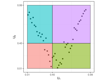
Figure 1: A sample from a copula $(U_{1},U_{2})$ with clear dependence, but where the overall sample correlation is close to zero. The dependence is captured by considering sample correlation of observations in different regions of the outcome space.

Lastly, we assume that $\varphi_{1},\dots,\varphi_{q}$ are linearly independent in Assumption 4 (iv) to avoid degeneracy of its empirical version, which we introduce in Section 4.4.

4.4 Test based on generalized correlation

In this section we will analyze in depth the conditional independence test resulting from basing the test $\psi_{n}$ in Definition 12 on the generalized correlation $\rho$. We will formulate the results in terms of a generic method for estimating conditional distribution functions in order to emphasize the generality of the method and illustrate the abstract assumptions needed for the test to be sound. Along the way we will explain when the assumptions are satisfied for the quantile regression based estimator $\hat{F}^{(m,n)}$ that we developed in Section 3.

With $\rho$ the generalized correlation between $U_{1}$ and $U_{2}$ defined in terms of a function $\varphi$ satisfying Assumption 4 we let $\rho_{n}:[0,1]^{2n}\to\mathbb{R}^{q\times q}$ be its corresponding empirical version:

$$\rho_{n}((u_{i},v_{i})_{i=1}^{n}):=\frac{1}{n}\sum_{i=1}^{n}\varphi(u_{i})\varphi(v_{i})^{T}.$$ (7)

Soundness of a test based on $\rho_{n}$ depends on consistency of the estimators $\hat{F}_{X\mid Z}^{(n)}$ and $\hat{F}_{Y\mid Z}^{(n)}$. Recall that we by $\mathcal{T}_{1},\dots,\mathcal{T}_{q}$ denote the supports of $\varphi_{1},\dots,\varphi_{q}$. Let $\tau_{\min}:=\inf(\mathcal{T}_{1}\cup\cdots\cup\mathcal{T}_{q})>0$ and $\tau_{\max}:=\sup(\mathcal{T}_{1}\cup\cdots\cup\mathcal{T}_{q})<1$, and then define $\mathcal{T}:=[\tau_{\min},\tau_{\max}]$. As in Section 3.2 we let the norm $\|\cdot\|_{\mathcal{T},\infty}$ be given by

$$\|f(t,z)\|_{\mathcal{T},\infty}=\sup_{z\in[0,1]^{d}}\sup_{t\in Q_{X\mid Z}(\mathcal{T}\mid z)}|f(t,z)|$$

when $X$ given $Z$ is the conditional distribution of interest. Similarly define $\|\cdot\|_{\mathcal{T},\infty}^{\prime}$ by

$$\|f(t,z)\|_{\mathcal{T},\infty}^{\prime}=\sup_{z\in[0,1]^{d}}\sup_{t\in Q_{Y\mid Z}(\mathcal{T}\mid z)}|f(t,z)|.$$

Then we have the following assumption on our estimators.

Assumption 5

For each distribution $P\in\mathcal{P}_{0}$ there exist deterministic rate functions $g_{P}$ and $h_{P}$ tending to zero as $n\to\infty$ and functions $\xi,\xi^{\prime}:[0,1]\times[0,1]^{d}\to\mathbb{R}$ such that

• $\|F_{X\mid Z}-\hat{F}_{X\mid Z}^{(n)}\|_{\mathcal{T},\infty}\in\mathcal{O}_{P}(g_{P}(n))$ and $\|F_{Y\mid Z}-\hat{F}_{Y\mid Z}^{(n)}\|_{\mathcal{T},\infty}^{\prime}\in\mathcal{O}_{P}(h_{P}(n))$.

• $||\xi-\hat{F}^{(n)}_{X\mid Z}||_{\mathcal{T}^{c},\infty}\in\mathcal{O}_{P}(g_{P}(n))$ and $||\xi^{\prime}-\hat{F}^{(n)}_{Y\mid Z}||_{\mathcal{T}^{c},\infty}^{\prime}\in\mathcal{O}_{P}(h_{P}(n))$.

Assumption 5 (i) states that our estimators $\hat{F}^{(n)}_{X\mid Z}$ and $\hat{F}^{(n)}_{Y\mid Z}$ are consistent with rates $g_{P}$ and $h_{P}$ over the conditional $\mathcal{T}$-quantiles in their respective conditional distributions. This is the result of Theorem 5 regarding our quantile regression based estimator $\hat{F}^{(m,n)}$ when $\mathcal{T}$ as above is taken as the set of potential quantile regression levels.

Assumption 5 (ii) is an assumption on the behavior of our estimator in the tails of the conditional distribution, i.e., over the conditional $\mathcal{T}^{c}$-quantiles. Here we do not assume consistency, but we do assume that the limit for $n\to\infty$ exists, and that our estimators are convergent to their limits with rates $g_{P}$ and $h_{P}$ respectively. This assumption is satisfied by our quantile regression based estimator $\hat{F}^{(m,n)}$ whenever it satisfies Assumption 5 (i).

With this assumption we first establish the asymptotic distribution of the test statistic

$$\hat{\rho}_{n}:=\rho_{n}\left((\hat{U}_{1,i},\hat{U}_{2,i})_{i=1}^{n}\right)=\frac{1}{n}\sum_{i=1}^{n}\varphi(\hat{U}_{1,i})\varphi(\hat{U}_{2,i})^{T}$$ (8)

under the hypothesis of conditional independence. Below we use $\Rightarrow_{P}$ to denote convergence in distribution with respect to $P$.

Theorem 14

Suppose that Assumption 5 is satisfied with rate functions $g_{P}$ and $h_{P}$ such that $\sqrt{n}g_{P}(n)h_{P}(n)\to 0$ as $n\to\infty$ for each $P\in\mathcal{P}_{0}$. Then the statistic $\hat{\rho}_{n}$ given by (8) satisfies

$$\sqrt{n}\hat{\rho}_{n}\Rightarrow_{P}\mathcal{N}(0,\Sigma\otimes\Sigma)$$

for each fixed $P\in\mathcal{H}_{0}$. The asymptotic covariance matrix is given by

$$\Sigma_{k,s}=\int_{0}^{1}\varphi_{k}(u)\varphi_{s}(u)\mathrm{d}u$$

for $k,s=1,\dots,q$ and does not depend on $P$.

If the rate functions are $g_{P}(n)=n^{-a}$ and $h_{P}(n)=n^{-b}$, then we require that $a+b>1/2$. Thus convergence slightly faster than rate $n^{-1/4}$ for both estimators is sufficient, but there can also be a tradeoff between the rates. Interestingly, Theorem 14 does not require sample splitting for the estimation of the conditional distribution function and computation of the test statistic. This is due to the fact that we are only interested in the asymptotic distribution under conditional independence. A similar phenomenon was found by Shah and Peters (2020), when they proved asymptotic normality of their Generalised Covariance Measure under conditional independence.

According to Corollary 9, the requirement $\sqrt{n}g_{P}(n)h_{P}(n)\to 0$ is satisfied for our quantile regression based estimator $\hat{F}^{(m,n)}$, if the quantile regression model (3) of Section 3.5 is valid for both $X$ given $Z$ and $Y$ given $Z$ for some continuous transformations $h_{1}:[0,1]^{d}\to\mathbb{R}^{p_{1}}$ and $h_{2}:[0,1]^{d}\to\mathbb{R}^{p_{2}}$ and Assumption 3 is satisfied with $s_{1},s_{2},p_{1},p_{2},n\to\infty$ such that

$$\sqrt{n}\cdot\sqrt{\frac{s_{1}\log(p_{1}\vee n)}{n}}\cdot\sqrt{\frac{s_{2}\log(p_{2}\vee n)}{n}}=\sqrt{\frac{s_{1}s_{2}\log(p_{1}\vee n)\log(p_{2}\vee n)}{n}}\to 0$$

where $s_{1}=\sup_{\tau\in\mathcal{T}}\|\beta_{1,\tau}\|_{0}$ and $s_{2}=\sup_{\tau\in\mathcal{T}}\|\beta_{2,\tau}\|_{0}$ are the sparsities of the model parameters.

With the test statistic

$$T_{n}:=\|\Sigma^{-1/2}\hat{\rho}_{n}\Sigma^{-1/2}\|_{F}^{2},$$ (9)

where $\|\cdot\|_{F}$ denotes the Frobenius norm, we have the following corollary of Theorem 14.

Corollary 15

Let the condition of Theorem 14 be satisfied and let $T_{n}$ be given by (9). Then it holds that

$$nT_{n}\Rightarrow_{P}\chi^{2}_{q^{2}}$$

for each fixed $P\in\mathcal{H}_{0}$.

In view of Theorem 14 and Corollary 15 we define the following conditional independence test based on the generalized correlation.

Definition 16

Let $\alpha\in(0,1)$ be a desired significance level and $T_{n}$ the test statistic (9). Then we let $\hat{\Psi}_{n}$ be the test given by

$$\hat{\Psi}_{n}=1(T_{n}>n^{-1}z_{1-\alpha})$$

where $z_{1-\alpha}$ is the $(1-\alpha)$-quantile of a $\chi^{2}_{q^{2}}$-distribution.

Control of the asymptotic pointwise level is then an easy corollary of Corollary 15.

Corollary 17

Suppose that Assumption 5 is satisfied with rate functions $g_{P}$ and $h_{P}$ such that $\sqrt{n}g_{P}(n)h_{P}(n)\to 0$ as $n\to\infty$ for each $P\in\mathcal{P}_{0}$. Then the test $\hat{\Psi}_{n}$ given by Definition 16 has asymptotic pointwise level over $\mathcal{H}_{0}$, i.e.,

$$\limsup_{n\to\infty}E_{P}(\hat{\Psi}_{n})=\alpha$$

for each fixed $P\in\mathcal{H}_{0}$.

This shows that the test achieves correct level given consistency of the estimators $\hat{F}^{(n)}_{X\mid Z}$ and $\hat{F}^{(n)}_{Y\mid Z}$ with suitably fast rates. To obtain results on power of the test $\hat{\Psi}_{n}$ we only need to understand how $\hat{\rho}_{n}$ converges in probability and not its entire asymptotic distribution.

Theorem 18

The test statistic $\hat{\rho}_{n}$ given by (8) satisfies

$$\hat{\rho}_{n}\stackrel{{\scriptstyle P}}{{\longrightarrow}}\rho$$

for each fixed $P\in\mathcal{P}_{0}$ under Assumption 5.

One may note that the theorem does not require that the rate functions $g_{P}$ and $h_{P}$ converge to zero at a certain rate. Let $\mathcal{A}_{0}\subseteq\mathcal{Q}_{0}$ be the subset of alternatives for which $\rho_{k\ell}\neq 0$ for at least one combination of $k,\ell=1,\dots,q$. Then we have the following corollary of Theorem 18, which exploits that $nT_{n}$ diverges in probability whenever $P\in\mathcal{A}_{0}$.

Corollary 19

For each level $\alpha\in(0,1)$ the test $\hat{\Psi}_{n}$ given by Definition 16 has asymptotic pointwise power against $\mathcal{A}_{0}$, i.e.,

$$\liminf_{n\to\infty}E_{P}(\hat{\Psi}_{n})=1$$

for each fixed $P\in\mathcal{A}_{0}$ under Assumption 5.

Let us discuss the alternatives the test has power against. Firstly, note that we always have the implications

$$X\mathrel{\text{\scalebox{1.07}{$\perp\mkern-10.0mu\perp$}}}Y\mid Z\quad\Rightarrow\quad U_{1}\mathrel{\text{\scalebox{1.07}{$\perp\mkern-10.0mu\perp$}}}U_{2}\quad\Rightarrow\quad\rho=0$$

However, none of the reverse implications are in general true. We do, however, have the following result stating a sufficient condition for the reverse implication of the first statement.

Proposition 20

Assume that $(U_{1},U_{2})\mathrel{\text{\scalebox{1.07}{$\perp\mkern-10.0mu\perp$}}}Z$. Then $X\mathrel{\text{\scalebox{1.07}{$\perp\mkern-10.0mu\perp$}}}Y\mid Z$ if and only if $U_{1}\mathrel{\text{\scalebox{1.07}{$\perp\mkern-10.0mu\perp$}}}U_{2}$.

This means that if $Z$ only affects the marginal distributions of $X$ and $Y$, then independence in the partial copula implies conditional independence. This is known as the simplifying assumption in the copula literature (Gijbels et al., 2015; Spanhel and Kurz, 2015). Naturally, $U_{1}\centernot{\mathrel{\text{\scalebox{1.07}{$\perp\mkern-10.0mu\perp$}}}}U_{2}$ always implies $X\centernot{\mathrel{\text{\scalebox{1.07}{$\perp\mkern-10.0mu\perp$}}}}Y\mid Z$, so the simplifying assumption is not a necessary condition for our test to have power, but it does give some intuition about a subset of distributions for which the partial copula completely characterizes conditional independence. However, an unavoidable limitation of the method is that it can never have power against alternatives for which $U_{1}\mathrel{\text{\scalebox{1.07}{$\perp\mkern-10.0mu\perp$}}}U_{2}$ but $X\centernot{\mathrel{\text{\scalebox{1.07}{$\perp\mkern-10.0mu\perp$}}}}Y\mid Z$.

Turning to the second implication, Corollary 19 tells us that we have power against alternatives for which $\rho_{k\ell}\neq 0$ for some $k,\ell=1,\dots,q$. However, not all types of dependencies can be detected in this fashion, and it is possible that $\rho=0$, while $U_{1}\centernot{\mathrel{\text{\scalebox{1.07}{$\perp\mkern-10.0mu\perp$}}}}U_{2}$. A test based on $\rho$ will not have power against such an alternative. For an abstract interpretation of the generalized correlation $\rho$ we refer to Section 4.3. In Section 4.6 we introduce a concrete generalized correlation and elaborate on its interpretation.

Finally, basing the test on values of $T_{n}$ is natural since the asymptotic behaviour is readily available through Theorem 14, but other transformations of $\hat{\rho}_{n}$ could be considered such as taking the coordinatewise absolute maximum $\max_{k,l}|(\Sigma^{-1/2}\hat{\rho}_{n}\Sigma^{-1/2})_{k,l}|=\|\Sigma^{-1/2}\hat{\rho}_{n}\Sigma^{-1/2}\|_{\infty}$.

4.5 Uniform level and power results

The level and power results of Section 4.4 are pointwise over the space of hypotheses and alternatives, i.e., they state level and power of the test when fixing a distribution $P$. In this section we describe how these results can be extended to hold uniformly by strengthening the statements in Assumption 5 to hold uniformly.

Assumption 6

For $\mathcal{P}_{0}\subset\mathcal{P}$ there exist deterministic rate functions $g$ and $h$ tending to zero as $n\to\infty$ and functions $\xi,\xi^{\prime}:[0,1]\times[0,1]^{d}\to\mathbb{R}$ such that

• $\|F_{X\mid Z}-\hat{F}_{X\mid Z}^{(n)}\|_{\mathcal{T},\infty}\in\mathcal{O}_{\mathcal{P}_{0}}(g(n))$ and $\|F_{Y\mid Z}-\hat{F}_{Y\mid Z}^{(n)}\|_{\mathcal{T},\infty}^{\prime}\in\mathcal{O}_{\mathcal{P}_{0}}(h(n))$.

• $||\xi-\hat{F}^{(n)}_{X\mid Z}||_{\mathcal{T}^{c},\infty}\in\mathcal{O}_{\mathcal{P}_{0}}(g(n))$ and $||\xi^{\prime}-\hat{F}^{(n)}_{Y\mid Z}||_{\mathcal{T}^{c},\infty}^{\prime}\in\mathcal{O}_{\mathcal{P}_{0}}(h(n))$.

As before we note that Assumption 6 (i) is the result of Theorem 7 regarding our quantile regression based estimator $\hat{F}^{(m,n)}$. Moreover, Assumption 6 (ii) is valid for $\hat{F}^{(m,n)}$ whenever it satisfies Assumption 6 (i).

We will now describe the extensions of Theorem 14 and Theorem 18 that can be obtained under Assumption 6. Below we write $\Rightarrow_{\mathcal{M}}$ to denote uniform convergence in distribution over a set of distributions $\mathcal{M}$, and we use $\to_{\mathcal{M}}$ to denote uniform convergence in probability over $\mathcal{M}$. We refer to Appendix B for the formal definitions.

Theorem 21

Let $\hat{\rho}_{n}$ be the statistic given by (8). Then we have:

• Under Assumption 6 with rate functions satisfying $\sqrt{n}g(n)h(n)\to 0$ it holds that

  $$\sqrt{n}\hat{\rho}_{n}\Rightarrow_{\mathcal{H}_{0}}\mathcal{N}(0,\Sigma\otimes\Sigma)$$

  where $\Sigma$ is as in Theorem 14.

• Under Assumption 6 it holds that $\hat{\rho}_{n}\to_{\mathcal{P}_{0}}\rho$.

As a straightforward corollary of Theorem 21 (i) we get the following uniform level result.

Corollary 22

The test $\hat{\Psi}_{n}$ given by Definition 16 has asymptotic uniform level over $\mathcal{H}_{0}$, i.e.,

$$\limsup_{n\to\infty}\sup_{P\in\mathcal{H}_{0}}E_{P}(\hat{\Psi}_{n})=\alpha,$$

given that Assumption 6 is satisfied with $\sqrt{n}g(n)h(n)\to 0$ as $n\to\infty$.

The pointwise power result of Theorem 19 does not extend directly to a uniform version in the same way as the level result. For $\lambda>0$ we let $\mathcal{A}_{\lambda}\subset\mathcal{Q}_{0}$ be the set of alternatives for which $|(\rho_{P})_{k\ell}|>\lambda$ for at least one combination of $k,\ell=1,\dots,q$, where we emphasize that $\rho_{P}$ depends on the distribution $P$. We then have the following uniform power result as a corollary of Theorem 21 (ii).

Corollary 23

For all fixed levels $\alpha\in(0,1)$ the test $\hat{\Psi}_{n}$ given by Definition 16 has asymptotic uniform power against $\mathcal{A}_{\lambda}$ for each $\lambda>0$, i.e.,

$$\liminf_{n\to\infty}\inf_{P\in\mathcal{A}_{\lambda}}E_{P}(\hat{\Psi}_{n})=1,$$

under Assumption 6.

The reason we need to restrict to the class of alternatives $\mathcal{A}_{\lambda}$ for a fixed $\lambda>0$ is the following. If the infimum is taken over $\mathcal{A}_{0}$, then there could exist a sequence $(P_{m})_{m=1}^{\infty}\subset\mathcal{A}_{0}$ of distributions such that $(\rho_{P_{m}})_{k\ell}\neq 0$ for each $m\geq 1$ but $(\rho_{P_{m}})_{k\ell}\to 0$ as $m\to\infty$. As a consequence $nT_{n}$ will not necessarily diverge in probability, which is crucial to the proof of the corollary. However, when restricting to $\mathcal{A}_{\lambda}$ we are ensured that $\inf_{P\in\mathcal{A}_{\lambda}}|(\rho_{P})_{k\ell}|\geq\lambda>0$ for at least one combination of $k,\ell=1,\dots,q$.

We note that these uniform level and power results are not in contradiction with the impossibility result of Shah and Peters (2020) mentioned in Section 1 because our results apply to a restricted set of distributions, $\mathcal{P}_{0}$, where the conditional distribution functions are estimable with sufficiently fast rate.

4.6 Trimmed Spearman correlation

We will now define a specific family of functions $\varphi$ defining the generalized correlation that can be shown to satisfy Assumption 4, which results in trimmed versions of the expected conditional Spearman correlation. As mentioned in Section 4.3, ignoring Assumption 4 (i), we could consider

$$\varphi_{k}(u)=\varphi_{\ell}(u)=\sqrt{12}\left(u-\frac{1}{2}\right)$$ (10)

for $u\in[0,1]$ which results in $\rho_{k\ell}$ being the expected conditional Spearman correlation of $X$ and $Y$ given $Z$ with respect to the distribution of $Z$. Drawing inspiration from (10) we define a class of functions $\varphi:[0,1]\to\mathbb{R}^{q}$ by letting

$$\varphi_{k}(u)=c_{k}(u-m_{k})\sigma_{k}(u)$$ (11)

such that each $\varphi_{k}:[0,1]\to\mathbb{R}$ is determined by a Lipschitz continuous function $\sigma_{k}:[0,1]\to\mathbb{R}$ with the support $\mathcal{T}_{k}$ of $\sigma_{k}$ a compact interval in $(0,1)$, $\int_{0}^{1}\sigma_{k}(u)\mathrm{d}u=1$ and

$$m_{k}=\int u\sigma_{k}(u)\mathrm{d}u\quad\text{and}\quad c_{k}=\left(\int(u-m_{k})^{2}\sigma_{k}(u)^{2}\mathrm{d}u\right)^{-1/2}.$$

The choice (11) satisfies Assumption 4 (i) – (iii) by construction, and if e.g. $\mathcal{T}_{k}\setminus\cup_{\ell\neq k}\mathcal{T}_{\ell}\neq\emptyset$ the functions are also linearly independent. We call the resulting generalized correlation $\rho$ a trimmed Spearman correlation, and we refer to the functions $\sigma_{k}$ as trimming functions. Note that if the supports $(\mathcal{T}_{k})_{k=1}^{q}$ of $(\sigma_{k})_{k=1}^{q}$ are choosen to be disjoint, then the covariance matrix $\Sigma$ of Theorem 14 is the identity matrix.

A starting point for choosing a trimming function $\sigma$ is the normalized indicator

$$u\mapsto(\lambda-\mu)^{-1}1_{[\mu,\lambda]}(u)$$ (12)

for $u\in[0,1]$ where $0<\mu<\lambda<1$ are trimming parameters. However, (12) is not a valid trimming function, since it is not Lipschitz. Therefore, we consider a simple linear approximation $\sigma:[0,1]\to\mathbb{R}$ given by

$$\sigma(u)=Kf(u)\quad\text{and}\quad f(u)=\begin{cases}1,\ &u\in[\mu+\delta,\lambda-\delta]\\ 0,\ &u\in[\mu,\lambda]^{c}\\ \delta^{-1}(u-\mu),\ &u\in[\mu,\mu+\delta)\\ \delta^{-1}(\lambda-u),\ &u\in(\lambda-\delta,\lambda]\end{cases}$$ (13)

and $K=(\lambda-\mu-\delta)^{-1}$. Here $0<\delta<(\lambda-\mu)/2$ is a fixed parameter that determines the accuracy of the approximation. It is elementary to verify that $\sigma$ given by (13) is a valid trimming function, i.e., $\sigma$ is Lipschitz continuous with $\int\sigma(u)\mathrm{d}u=1$ and support $[\mu,\lambda]\subset(0,1)$.

The interpretation of a generalised correlation $\rho$ based on $\varphi$ of the form (11) with trimming function $\sigma$ of the form (13) is as follows. The entry $\rho_{k\ell}$ is an approximation of the expected conditional Spearman correlation between the observations of $X$ and $Y$, respectively, that lie in the $\mathcal{T}_{k}$-quantile range of the distribution of $X$ given $Z$ and the $\mathcal{T}_{\ell}$-quantile range of the distribution of $Y$ given $Z$, respectively, with respect to the distribution of $Z$. The matrix $\rho$ then summarizes this type of dependence within different quantile ranges of $X$ and $Y$ given $Z$.

4.7 Practical considerations

Throughout Sections 4.4 and 4.5 we have analyzed our proposed test for conditional independence with an emphasis on modularity of the method regarding the choice of estimators $\hat{F}^{(n)}_{X\mid Z}$ and $\hat{F}^{(n)}_{Y\mid Z}$ of the conditional distribution functions and the choice of the function $\varphi$ that defines the generalized correlation $\rho$ of Section 4.3. This focus on the conceptual assumptions displays the generality of the method, but it also leaves the practitioner of conditional independence testing with a number of choices to be made. In this section we summarize a set of choices to make the method work out-of-the-box.

Throughout the paper we have assumed that all random variables take values in the unit interval, i.e., $(X,Y,Z)\in[0,1]^{d+2}$. This is not a restriction, since if e.g. $X\in\mathbb{R}$ we can always apply a strictly increasing, continuous transformation $t:\mathbb{R}\to[0,1]$ to obtain a new random variable $X^{\prime}=t(X)$ with values in $[0,1]$. Moreover, the initial conditional independence structure of $(X,Y,Z)$ is preserved since the transformation is marginal on $X$ and bijective. The transformation $t$ can be chosen to be e.g. the logistic function.

In principle, an arbitrary and fixed marginal transformation could be used for all variables, but we recommend to transform data to the unit interval via marginal empirical distribution functions. This results in transformed variables known in the copula literature as pseudo copula observations. The transformation creates dependence, similar to the dependence created by other common preprocessing techniques such as centering and scaling, which the theoretical analysis has not accounted for. We suggest, nevertheless, to use this preprocessing technique in practise, and in the simulation study in Section 5 we use pseudo copula observations since it reflects how a practitioner would transform the variables.

To estimate the conditional distribution functions $\hat{F}^{(m,n)}_{X\mid Z}$ and $\hat{F}^{(m,n)}_{Y\mid Z}$ using Definition 2, we suggest choosing $\tau_{\min}=0.01$ and $\tau_{\max}=0.99$ and form the equidistant grid $(\tau_{k})_{k=1}^{m}$ in $\mathcal{T}=[\tau_{\min},\tau_{\max}]$ with the number of gridpoints $m=\lceil\sqrt{n}\rceil$. We then suggest using a model of the form (3) for both the quantile regression model $Q_{X\mid Z}(\tau_{k}\mid\cdot)$ and $Q_{Y\mid Z}(\tau_{k}\mid\cdot)$ for each $k=1,\dots,m$, where the bases $h_{1}$ and $h_{2}$ can be chosen to be e.g. an additive B-spline basis for each component of $Z$.

To test the hypothesis of conditional independence we suggest using the $\hat{\Psi}_{n}$ from Definition 16 based on the estimated nonparametric residuals $(\hat{U}_{1,i},\hat{U}_{2,i})_{i=1}^{n}$. To this end we choose $q\geq 1$ and let $\tau_{\min}=\lambda_{0}<\cdots<\lambda_{q}=\tau_{\max}$ be an equidistant grid in $\mathcal{T}$. We then define the trimming function $\sigma_{k}$ to have the form (13) with trimming parameters $\lambda_{k}$ and $\lambda_{k+1}$ and approximation parameter $\delta=0.01\cdot(\lambda_{k+1}-\lambda_{k})$ for each $k=0,\dots,q-1$. We then define $(\sigma_{k})_{k=1}^{q}$ according to (11), compute the test statistic $\hat{\rho}_{n}$ using (8) and compute $\hat{\Psi}_{n}$ as in Definition 16 using a desired significance level $\alpha\in(0,1)$.

There are two non-trivial choices remaining. The first is the choice of bases $h_{1}$ and $h_{2}$ for the quantile regression models $Q_{X\mid Z}(\tau_{k}\mid z)=h_{1}(z)^{T}\beta_{\tau_{k}}$ and $Q_{Y\mid Z}(\tau_{k}\mid z)=h_{2}(z)^{T}\beta_{\tau_{k}}$. Here the practitioner needs to make a qualified model selection. We recommend using a flexible basis such as an additive B-spline basis, and perform penalized estimation using (4) to avoid overfitting. The second choice is the dimension of the generalized correlation $q\geq 1$, which corresponds to a choice of independence test in the partial copula. Note that the generalized correlation $\rho$ as above is defined for any $q\geq 1$, and there is conditional dependence, $X\centernot{\mathrel{\text{\scalebox{1.07}{$\perp\mkern-10.0mu\perp$}}}}Y\mid Z$, if there exists $q\geq 1$ for which $\rho\neq 0$. We suggest trying one or a few, small values, e.g. $q\in\{1,\dots,5\}$, and reject the hypothesis of conditional independence if one of the tests rejects the hypothesis, but of course be aware of multiple testing issues.

5 Simulation Study

In this section we examine the performance of our conditional independence test $\hat{\Psi}_{n}$ of Definition 16, when combining it with the quantile regression based conditional distribution function estimator $\hat{F}^{(m,n)}$ from Definition 2. Firstly, we verify the level and power results obtained in Section 4.4 and Section 4.5 empirically. Secondly, we compare the test with other conditional independence tests. The test was implemented in the R language (R Core Team, 2021) using the quantreg package (Koenker, 2021) as the backend for performing quantile regression. The implementation and code for producing the simulations can be obtained from https://github.com/lassepetersen/partial-copula-CI-test.

5.1 Evaluation method

We will evaluate the tests by their ability to hold level when data is generated from a distribution where conditional independence holds, and by their power when data is generated from a distribution where conditional independence does not hold. In order to make the results independent of a chosen significance level we will base the evaluation on the $p$-values of the tests.

If a test has valid level, then we expect the $p$-value to be asymptotically $\mathcal{U}[0,1]$-distributed. In Sections 5.3 and 5.4 we evaluate the level by a Kolmogorov-Smirnov (KS) statistics as a function of sample size $n$, which is independent of any specific significance level. A small KS statistic is an indication of valid level. To examine power we consider in Sections 5.3 and 5.4 the $p$-values of the test as a function of the sample size, where we expect the $p$-values to tend to zero under the alternative of conditional dependence. Here a small $p$-value is an indication of large power. In Section 5.5 we evaluate the power against a local alternative, which shrinks with the sample size $n$ toward the hypothesis of conditional independence with rate $n^{-\frac{1}{2}}$.

5.2 Data generating processes

This section gives an overview of the data generating processes that we use for benchmarking and comparison. The first category consists of data generating processes of the form

$$X=f_{1}(Z)+g_{1}(Z)\cdot\varepsilon_{1}\quad\text{and}\quad Y=f_{2}(Z)+g_{2}(Z)\cdot\varepsilon_{2}$$ (H)

where $f_{1},f_{2},g_{1},g_{2}:\mathbb{R}^{d}\to\mathbb{R}$ belong to some function class and $\varepsilon_{1},\varepsilon_{2}$ are independent errors. For data generating processes of type (H), conditional independence is satisfied. The second category consists of data generating processes of the form

$$X=f_{1}(Z)+g_{1}(Z)\cdot\varepsilon_{1}\quad\text{and}\quad Y=f_{2}(Z,X)+g_{2}(Z,X)\cdot\varepsilon_{2}$$ (A)

where again $f_{1},g_{1}:\mathbb{R}^{d}\to\mathbb{R}$ and $f_{2},g_{2}:\mathbb{R}^{d+1}\to\mathbb{R}$ belong to some function class and $\varepsilon_{1},\varepsilon_{2}$ are independent errors. Under data generating processes of type (A), conditional independence is not satisfied. We will consider four different data generating processes corresponding to different choices of functions $f_{1}$, $g_{1}$, $f_{2}$ and $g_{2}$ and error distributions.

• For data generating processes $\mathrm{H}_{1}$ and $\mathrm{A}_{1}$ we let

  $$f_{k}(w_{1},\dots,w_{d}) =\sum_{j=1}^{d}\beta_{1,k,j}w_{j}+\beta_{2,k,j}w_{j}^{2}$$

  $$g_{k}(w_{1},\dots,w_{d}) =\exp\left(-\left|\sum_{j=1}^{d}\alpha_{1,k,j}w_{j}+\alpha_{2,k,j}w_{j}^{2}\right|\right)$$

  for $k=1,2$ and real valued coefficients $(\alpha_{\ell,k,j},\beta_{\ell,k,j})_{\ell=1,2,k=1,2,j=1,\dots,d}$. Here each $Z_{j}\sim\mathcal{U}[-1,1]$ independently, $\varepsilon_{1}$ follows an asymmetric Laplace distribution with location $0$, scale $1$ and skewness $0.8$, and $\varepsilon_{2}$ follows a Gumpel distribution with location $0$ and scale $1$.

• For data generating processes $\mathrm{H}_{2}$ and $\mathrm{A}_{2}$ we let $g_{1}=g_{2}=1$ and

  $$f_{k}(w_{1},\dots,w_{d})=\sum_{j=1}^{d}\beta_{k,j}w_{j}$$

  for $k=1,2$ and real valued coefficients $(\beta_{k,j})_{k=1,2,j=1,\dots,d}$. Here each $Z_{j}\sim\mathcal{U}[-1,1]$ independently and both $\varepsilon_{1}$ and $\varepsilon_{2}$ follow a $\mathcal{N}(0,1)$-distribution independently.

• For data generating processes $\mathrm{H}_{3}$ and $\mathrm{A}_{3}$ we let $g_{1}=g_{2}=1$ and

  $$f_{k}(w_{1},\dots,w_{d})=\sum_{j=1}^{d}\beta_{1,k,j}w_{j}+\beta_{2,k,j}w_{j}^{2}$$

  for $k=1,2$ and real valued coefficients $(\beta_{\ell,k,j})_{\ell=1,2,k=1,2,j=1,\dots,d}$. Here each $Z_{j}\sim\mathcal{U}[-1,1]$ independently and both $\varepsilon_{1}$ and $\varepsilon_{2}$ follow a $\mathcal{N}(0,1)$-distribution independently.

• For data generating processes $\mathrm{H}_{4}$ and $\mathrm{A}_{4}$ we let $f_{1}=f_{2}=0$ and

  $$g_{k}(w_{1},\dots,w_{d})=\sum_{j=1}^{d}\beta_{1,k,j}w_{j}+\beta_{2,k,j}w_{j}^{2}$$

  for $k=1,2$ for real valued coefficients $(\beta_{\ell,k,j})_{\ell=1,2,k=1,2,j=1,\dots,d}$. Here each $Z_{j}\sim\mathcal{U}[-1,1]$ independently and both $\varepsilon_{1}$ and $\varepsilon_{2}$ follow a $\mathcal{N}(0,1)$-distribution independently.

Each time we simulate from data generating processes $\mathrm{H}_{1},\dots,\mathrm{H}_{4}$ we first draw the coefficients of the functions $f_{k},g_{k}$ from a $\mathcal{N}(0,1)$-distribution in order to make the results independent of a certain combination of parameters. When we simulate from the data generating processes $\mathrm{A}_{1},\mathrm{A}_{2}$ and $\mathrm{A}_{3}$ we first draw the coefficients of $f_{k},g_{k}$ to be either $-1$ or $1$ with equal probability in order to fix the signal to noise ratio between the predictors and responses. When simulating from $\mathrm{A}_{4}$ we simulate the coefficients of $g_{k}$ to be either $-5$ or $5$, because the conditional dependence lies in the variance for $\mathrm{A}_{4}$, and a stronger signal is needed to compare the power of the tests using the same samples sizes as for $\mathrm{A}_{1},\mathrm{A}_{2}$ and $\mathrm{A}_{3}$.

The data generating processes $\mathrm{H}_{2},\mathrm{H}_{3},\mathrm{H}_{4},\mathrm{A}_{2},\mathrm{A}_{3}$ and $\mathrm{A}_{4}$ can be shown to satisfy Assumption 3 that is needed for Corollary 9, since they are linear (in the parameters) location-scale models with bounded covariates (Belloni and Chernozhukov, 2011, Section 2.5). The processes $\mathrm{H}_{1}$ and $\mathrm{A}_{1}$ are not of this form, since $g_{1}$ and $g_{2}$ are nonlinear in the parameters. However, we include these in the simulation study to test the robustness of the test.

5.3 Level and power of partial copula test

In this section we examine the level and power properties of the test $\hat{\Psi}_{n}$. We examine the performance of the test on data generating processes $\mathrm{H}_{1}$ and $\mathrm{A}_{1}$ for dimensions $d\in\{1,5,10\}$ of $Z$. The test is performed as described in Section 4.7. As the quantile regression model we use an additive model with a B-spline basis of each variable with 5 degrees of freedom, and we try $q\in\{1,\dots,5\}$. The result of the simulations can be seen in Figure 2.

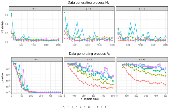
Figure 2: Top: KS statistic for equality with a $\mathcal{U}[0,1]$-distribution of the p-values of the two tests computed from 500 simulations from $\mathrm{H}_{1}$ for each combination of $n$ and $d$. Bottom: Average p-values of the two tests separately computed over 200 simulations from $\mathrm{A}_{1}$ for each combination of $n$ and $d$. Dashed line indicates the common significance level $0.05$. For visual purposes all $p$-values have been truncated at $10^{-10}$.

We observe that for $d=1$ all five tests obtain level asymptotically under $\text{H}_{1}$, while for higher dimension $d\in\{5,10\}$ the test with $q=4$ has minor problems holding level. We also see that the $p$-values for all five tests tend to zero as the sample size increases under $\text{A}_{1}$. The convergence rate of the $p$-value depends on the dimension $d$ such that a higher dimension gives a slower convergence rate. In conclusion we observe that our test holds level under a complicated data generating distribution ($\text{H}_{1}$), where there is a nonlinear conditional mean and variance dependence and skewed error distributions with super-Gaussian tails. Moreover, the test has power against the alternative of conditional dependence ($\text{A}_{1}$), however, for $d=1$ we see that $q=5$ gives the best power, while $q=1$ gives the best power for $d\in\{5,10\}$. The testing procedure also displays robustness to the fact that the quantile regression models are misspecified.

5.4 Comparison with other tests

We now compare the partial copula based test $\hat{\Psi}_{n}$ with other nonparametric tests. We will compare with a residual based method, since this is another class of conditional independence test based on nonparametric regression. In order to describe this test we let

$$R_{1,i}=X_{i}-\hat{f}(Z_{i})\ \quad\text{and}\quad R_{2,i}=Y_{i}-\hat{g}(Z_{i})$$

for $i=1,\dots,n$ be the residuals obtained when performing conditional mean regression $\hat{f}$ of $f(z)=E(X\mid Z=z)$ and $\hat{g}$ of $g(z)=E(Y\mid Z=z)$ obtained from a sample $(X_{i},Y_{i},Z_{i})_{i=1}^{n}$. We compare the following conditional independence tests:

• GCM: The Generalised Covariance Measure which tests for vanishing correlation between the residuals $R_{1}$ and $R_{2}$ given as above (Shah and Peters, 2020).

• NPN correlation: Testing for vanishing partial correlation in a nonparanormal distribution (Harris and Drton, 2013). This is a generalization of the partial correlation, which assumes a Gaussian dependence structure, but allows for arbitrary marginal distributions.

• PC: Our partial copula based test $\hat{\Psi}_{n}$ for $q\in\{1,3,5\}$ as described in Section 4.7.

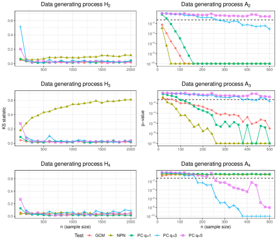
Figure 3: Left column: KS statistic for equality with a $\mathcal{U}[0,1]$-distribution of the p-values of the five tests computed from 500 simulations from $\mathrm{H}_{2},\mathrm{H}_{3}$ and $\mathrm{H}_{4}$, respectively, for each sample size $n$. Right column: Average p-values of the five tests separately computed over 200 simulations from $\mathrm{A}_{2},\mathrm{A}_{3}$ and $\mathrm{A}_{4}$, respectively, for each sample size $n$. For all simulations the dimension is fixed at $d=3$. Dashed line indicates the common significance level $0.05$. For visual purposes all $p$-values have been truncated at $10^{-10}$.

We consider the behavior of the tests under $\mathrm{H}_{2},\mathrm{A}_{2},\mathrm{H}_{3},\mathrm{A}_{3},\mathrm{H}_{4}$ and $\mathrm{A}_{4}$. For fairness of comparison we choose our quantile and mean regression models to be the correct model class such that the tests perform at their oracle level, e.g., for $\mathrm{H}_{3}$ we fit additive models with polynomial basis of degree $2$. We fix the dimension $d$ of $Z$ to be $3$ in all simulations for simplicity. The results of the simulations can be seen in Figure 3.

Under $\text{H}_{2}$ all five tests hold level, and we see that the NPN test has greatest power against $\text{A}_{2}$ followed by the GCM and $\hat{\Psi}_{n}$ with $q=1$, while $\hat{\Psi}_{n}$ with $q\in\{3,5\}$ does not have much power against $\text{A}_{2}$. In order to intuitively understand the effect of $q$ see Figure 4. We see that in the estimated partial copula the dependence is captured by the overall correlation, while dividing $[\tau_{\min},\tau_{\max}]\times[\tau_{\min},\tau_{\max}]$ into subregions does not reveal finer dependence structure. Hence $q=1$ is suitable to detect the dependence for $\text{A}_{1}$.

Under $\text{H}_{3}$ both the GCM test and $\hat{\Psi}_{n}$ with $q\in\{1,3,5\}$ hold level, but the NPN test does not hold level under $\text{H}_{3}$, which is due to the nonlinear response-predictor relationship. However, since both the GCM and $\hat{\Psi}_{n}$ test takes the nonlinearity into account, they can effectively filter away the $Z$-dependence. The NPN test has greatest power against the alternative $\text{A}_{3}$ following by $\hat{\Psi}_{n}$ with $q=1$ and the GCM test. In Figure 4 we again see that the dependence in the estimated partial copula is described by the overall correlation, while dividing into subregions results a generalized correlation with elements that are close to zero, i.e., here $q=1$ is suitable for capturing the dependence.

Under $\text{H}_{4}$, all test hold level. Note that the NPN test holds level even though there is a nonlinear conditional variance relation, since this is still a nonparanormal distribution. We also see that neither the GCM test nor the NPN test has power against $\text{A}_{4}$, while $\hat{\Psi}_{n}$ has some power against $\text{A}_{4}$ with the greatest power for $q=3$. In Figure 4 we see that there is a clear dependence in the estimated partial copula, but that the overall correlation is close to zero. However, when dividing into subregions the generalized correlation is able to detect the dependencies in the tails of the distributions.

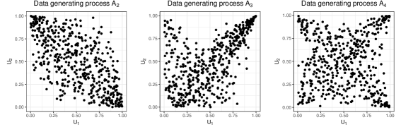
Figure 4: Estimated partial copula $(\hat{U}_{1,i},\hat{U}_{2,i})_{i=1}^{n}$ from one realization from each of the data generating processes $\text{A}_{2},\text{A}_{3}$ and $\text{A}_{4}$ for $d=3$ and $n=500$.

5.5 Power under local alternatives

Though GCM did not have power against the specific alternative $\text{A}_{4}$, it maintains level and it has power against a broad class of alternatives. To understand better when $\hat{\Psi}_{n}$ can be expected to have greater power than GCM, we consider a simulation, which is a small variation of the simulations presented in Section 5.2.

The dimension is fixed as $d=1$, $Z\sim\mathcal{U}([0,1])$ is uniformly distributed on $[0,1]$, $\varepsilon_{1}$, $\varepsilon_{2}$ and $W$ are independent and $\mathcal{N}(0,1)$-distributed, and

$$X=(\beta Z^{2}+1)\varepsilon_{1}+\gamma W\quad\text{and}\quad Y=(\beta Z^{2}+1)\varepsilon_{2}+\gamma W$$ (A)

for parameters $\beta,\gamma\in\mathbb{R}$. Conditionally on $Z$, the distribution of $(X,Y)$ is a bivariate Gaussian distribution, and $X$ and $Y$ are conditionally independent if and only if $\gamma=0$.

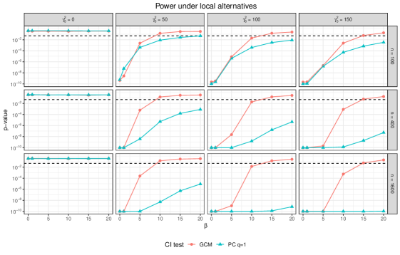
Figure 5: Average p-values of the three tests separately computed over 500 simulations for different values of the parameters $\beta$ and $\gamma_{0}$ and different sample sizes $n$. The value $\gamma_{0}^{2}=0$ is equivalent to conditional independence. Other values correspond to the local alternatives $\gamma^{2}=\gamma_{0}^{2}/\sqrt{n}$. The values of $\beta$ determine the amount of heterogeneity of the mean regression residual variances with $\beta=0$ meaning constant residual variance and $\beta=20$ meaning substantial heterogeneity. Dashed line indicates the common significance level $0.05$. For visual purposes all $p$-values have been truncated at $10^{-10}$.

We examine level and power by simulating 500 data sets for sample sizes $n\in\{100,400,1600\}$ and all combinations of parameters $\beta\in\{0,1,5,10,15,20\}$, and local alternatives

$$\gamma^{2}=\frac{\gamma_{0}^{2}}{\sqrt{n}}$$

for $\gamma_{0}^{2}\in\{0,50,100,150\}$. Note that $f(z)=E(X\mid Z=z)=0$ and $g(z)=E(Y\mid Z=z)=0$, which is exploited for GCM instead of estimating $f$ and $g$. This should only increase the power of GCM relative to fitting any model of the conditional expectations. We perform the test $\hat{\Psi}_{n}$ as described in Section 4.7 using $q=1$, and the quantile regression model is fitted using a polynomial basis of degree 2.

Figure 5 shows the results of the simulation. Both GCM and $\hat{\Psi}_{n}$ maintain level for $\gamma_{0}^{2}=0$. $\hat{\Psi}_{n}$ has comparable or superior power relative to GCM in all other cases. Both tests have decreasing power as a function of $\beta$, but $\hat{\Psi}_{n}$ maintains power even for large values of $\beta$, where GCM has almost no power. The power of $\hat{\Psi}_{n}$ against the local alternatives increases with the sample size, which shows how the increased precision for larger samples of the quantile regression based distribution functions improves power. We do not see the same for GCM, partly because no mean value model is fitted.

As $\beta$ quantifies the conditional variance heterogeneity of $X$ and $Y$ given $Z$, we conclude that though GCM remains a valid test under conditional variance heterogeneity, its test statistic does not adequately account for the heterogeneity, and GCM has inferior power under local alternatives when compared to $\hat{\Psi}_{n}$.

6 Discussion

The first main contribution of this paper is an estimator of conditional distribution functions $\hat{F}^{(m,n)}$ based on quantile regression. We have shown that the estimator is pointwise (uniformly) consistent over a set of distributions $\mathcal{P}_{0}\subset\mathcal{P}$ given that the quantile regression procedure is pointwise (uniformly) consistent over $\mathcal{P}_{0}$. Moreover, we showed that the convergence rate of the quantile regression procedure can be transferred directly to the estimator $\hat{F}^{(m,n)}$.

The second main contribution of this paper is an analysis of a nonparametric test for conditional independence based on the partial copula construction. We introduced a class of tests given in terms of a generalized correlation dependence measure $\rho$ with the leading example being a trimmed version of the Spearman correlation. We showed that the test achieves asymptotic pointwise (uniform) level and power over $\mathcal{P}_{0}$ given that the conditional distribution function estimators are pointwise (uniformly) consistent over $\mathcal{P}_{0}$ with rate functions $g_{P}$ and $h_{P}$ satisfying $\sqrt{n}g_{P}(n)h_{P}(n)\to 0$. The partial copula has previously been considered for conditional independence testing in the literature, however, to the best of our knowledge, the results presented here are the first to explicitly connect the consistency requirements of the conditional distribution function estimators to level and power properties of the test.

Lastly, we established through a simulation study that the proposed test is sound under complicated data generating distributions, and that it has power comparable to or even better than other state-of-the-art nonparametric conditional independence tests. In particular, we demonstrated that our test has superior power against alternatives with variance heterogeneity between $X$ and $Y$ given $Z$ when compared to conditional independence tests based on conventional residuals. We note that due to Daudin’s lemma, tests based on conventional residuals can obtain power against any alternative if suitable transformations of $X$ and $Y$ are considered. In particular, if $X^{2}$ and $Y^{2}$ were used in our simulation study, GCM would have power against $\text{A}_{4}$. We tested the use of GCM in combination with $X^{2}$ and $Y^{2}$ in all our simulations (data not shown), and though it had some power against $\text{A}_{4}$, it was comparable to or inferior to just using GCM in all other simulations. Thus to obtain good power properties, the specific choice of transformation appears important and to depend on the data generating distribution.

An important point about the test is the rate requirement $\sqrt{n}g_{P}(n)h_{P}(n)\to 0$ needed to achieve asymptotic level. The product structure means that the test is sound under quantile regression models with slower consistency rates than the usual parametric $n^{-1/2}$-rate. This opens up the methodology to nonparametric machine learning models. An interesting direction of research would be to empirically assess the performance of the test using machine learning inspired quantile regression models, such as deep neural networks, where explicit consistency rates are not available. We hypothesize that the method will still perform well in these scenarios due to the weak consistency requirement.

In this paper we have considered univariate $X$ and $Y$. A possible extension of the test is to allow $X\in[0,1]^{r_{1}}$ and $Y\in[0,1]^{r_{2}}$ with $r_{1},r_{2}\geq 1$, and then consider the nonparametric residual $U_{1}\in[0,1]^{r_{1}}$ of $X$ given $Z$ by performing coordinatewise probability integral transformations $U_{1,k}=F_{X_{k}\mid Z}(X_{k}\mid Z)$ for $k=1,\dots,r_{1}$, and similarly for constructing the nonparametric residual $U_{2}\in[0,1]^{r_{2}}$ of $Y$ given $Z$. Conditional independence $X\mathrel{\text{\scalebox{1.07}{$\perp\mkern-10.0mu\perp$}}}Y\mid Z$ then implies pairwise independence of $U_{1,k}$ and $U_{2,l}$ for each $k=1,\ldots,r_{1}$ and $l=1,\ldots,r_{2}$. Combining our proposed test statistics for each such pair yields an $r_{1}r_{2}q^{2}$-dimensional test statistic, whose distribution under the hypothesis of conditional independence will be asymptotically Gaussian with mean 0. Its covariance matrix will only be partially known, though, due to the potential dependence between the pairs, but the unknown part could be estimated from the estimated nonparametric residuals. The multivariate statistic could be aggregated into a univariate test statistic in various ways, e.g. by a quadratic transformation as in (9), or by the maximum of the absolute values of its coordinates. In the low-dimensional case for fixed $r_{1}$ and $r_{2}$ our results would carry over immediately, and we expect that using the maximum could lead to high-dimensional results similar to Theorem 9 by Shah and Peters (2020).

A key property of the partial copula is that the nonparametric residuals $U_{1}$ and $U_{2}$ are independent under conditional independence and not only uncorrelated, which is the case for conventional residuals in additive noise models. Therefore, an important question is whether asymptotic level and power guaranties can be proven, when combining the partial copula with more general independence tests. In this paper we have focused on dependence measures of the form $\rho=E_{P}(\varphi(U_{1})\varphi(U_{2})^{T})$ and tests based on

$$\hat{\rho}_{n}=\frac{1}{n}\sum_{i=1}^{n}\varphi(\hat{U}_{1,i})\varphi(\hat{U}_{2,i})^{T}$$

because it gives a flexible and general test for independence in the partial copula, it can be computed in linear time in the size of data, and most importantly its asymptotic theory is standard and easy to establish and apply. It also clearly illustrates the transfer of consistency of the conditional distribution function estimators to properties of the test. It is ongoing work to establish a parallel asymptotic theory for dependence measures of the form $\theta=E_{P}(h(U_{1},U_{2}))$, where $h$ is a kernel function, and whose estimators are $U$-statistics. This could potentially yield more powerfull tests against complicated alternatives of conditional dependence, but at the prize of increased computational complexity.

Acknowledgments

This work was supported by a research grant (13358) from VILLUM FONDEN.

A Proofs

This appendix gives proofs of the main results of the paper. Throughout the proofs we will ignore the dependence of certain terms on the sample size to ease notation, e.g. we write $\hat{U}_{1,i}$ instead of $\hat{U}^{(n)}_{1,i}$ and $\hat{q}_{k,z}$ instead of $\hat{q}_{k,z}^{(n)}$.

A.1 Proof of Proposition 1

We need to bound the supremum

$$||F-\tilde{F}^{(m)}||_{\mathcal{T},\infty}=\sup_{z\in[0,1]^{d}}\sup_{t\in Q(\mathcal{T}\mid z)}|F(t\mid z)-\tilde{F}^{(m)}(t\mid z)|.$$

First we fix $z\in[0,1]^{d}$ and inspect the inner supremum. By construction we have

$$F(q_{k,z}\mid z)=\tilde{F}^{(m)}(q_{k,z}\mid z)=\tau_{k}$$

for $k=1,\dots,m$. Furthermore, since both $F$ and $\tilde{F}^{(m)}$ are continuous and increasing in $t\in[0,1]$ we have that

$$\sup_{t\in[q_{k,z},q_{k+1,z}]}|F(t\mid z)-\tilde{F}^{(m)}(t\mid z)|\leq\tau_{k+1}-\tau_{k}$$

for each $k=1,\dots,m-1$. Since $Q(\mathcal{T}\mid z)=[q_{\min,z},q_{\max,z}]=\bigcup_{k=1}^{m-1}[q_{k,z},q_{k+1,z}]$ we now have

$$\sup_{t\in Q(\mathcal{T}\mid z)}|F(t\mid z)-\tilde{F}^{(m)}(t\mid z)| =\max_{k=1,\dots,m-1}\sup_{t\in[q_{k,z},q_{k+1,z}]}|F(t\mid z)-\tilde{F}^{(m)}(t\mid z)|$$

$$\leq\max_{k=1,\dots,m-1}(\tau_{k+1}-\tau_{k})=\kappa_{m}.$$

The result now follows from taking supremum over $z\in[0,1]^{d}$ as the right hand side of the inequality does not depend on $z$. $\square$

A.2 Proof of Proposition 4

We need to bound the supremum

$$\|\tilde{F}^{(m)}-\hat{F}^{(m,n)}\|_{\mathcal{T},\infty}=\sup_{z\in[0,1]^{d}}\sup_{t\in Q(\mathcal{T}\mid z)}|\tilde{F}^{(m)}(t\mid z)-\hat{F}^{(m,n)}(t\mid z)|.$$

Our proof strategy is the following. First we evaluate the inner supremum over $t\in Q(\mathcal{T}\mid z)$ analytically to obtain a bound in terms of the quantile regression prediction error. Then we will evaluate the outer supremum over $z\in[0,1]^{d}$ and use the assumed consistency from Assumption 1. First define the two quantities

$$A(m,n,z):=\kappa_{m}\cdot\frac{\max_{k=1,\dots,m}|q_{k,z}-\hat{q}^{(n)}_{k,z}|}{\min_{k=1,\dots,m-1}(q_{k+1,z}-q_{k,z})}$$

and

$$B(m,n,z):=\kappa_{m}\cdot\frac{\max_{k=1,\dots,m}|q_{k,z}-\hat{q}^{(n)}_{k,z}|}{\min_{k=1,\dots,m-1}(\hat{q}^{(n)}_{k+1,z}-\hat{q}^{(n)}_{k,z})}.$$

We then have the following key result regarding the inner supremum over $t\in Q(\mathcal{T}\mid z)$.

Proposition 24

Let Assumption 1 (i) be satisfied. Then for all $P\in\mathcal{P}_{0}$ and $\varepsilon>0$ there exists $N\geq 1$ such that for all $n\geq N$,

$$\sup_{t\in Q(\mathcal{T}\mid z)}|\tilde{F}^{(m)}(t\mid z)-\hat{F}^{(m,n)}(t\mid z)|\leq\max\{A(m,n,z),B(m,n,z)\}$$

for all $z\in[0,1]^{d}$ and all grids $(\tau_{k})_{k=1}^{m}$ in $\mathcal{T}$ with probability at least $1-\varepsilon$.

We need a number of auxilliary results before proving Proposition 24. We start by proving the following key lemma that reduces the number of distinct cases of relative positions of the true conditional quantiles $q_{k,z}$ and the estimated conditional quantiles $\hat{q}_{k,z}$.

Lemma 25

Let Assumption 1 (i) be satisfied. Then for each $P\in\mathcal{P}_{0}$ and $\varepsilon>0$ there exists $N\geq 1$ such that for all $n\geq N$ we have that $\hat{q}_{k,z}\in(q_{k-1,z},q_{k+1,z})$ for each $k=1,\dots,m$ and $z\in[0,1]^{d}$ and for all grids $(\tau_{k})_{k=1}^{m}$ in $\mathcal{T}$ with probability at least $1-\varepsilon$.

Proof  Fix a distribution $P\in\mathcal{P}_{0}$. Let $\mathcal{G}$ be the set of all grids $(\tau_{k})_{k=1}^{m}$ in $\mathcal{T}$. Then

$$\sup_{\mathcal{G}}\sup_{z\in[0,1]^{d}}\max_{k=1,\dots,m}|q_{k,z}-\hat{q}_{k,z}^{(n)}|\leq\sup_{z\in[0,1]^{d}}\sup_{\tau\in\mathcal{T}}|Q(\tau\mid z)-\hat{Q}^{(n)}(\tau\mid z)|\stackrel{{\scriptstyle P}}{{\to}}0$$

under Assumption 1 (i). Since $q_{k,z}\in(q_{k-1,z},q_{k+1,z})$ for each $k=1,\dots,m$ and $z\in[0,1]^{d}$ for all grids $(\tau_{k})_{k=1}^{m}$ in $\mathcal{T}$ the result follows.  

Next we have some lemmas giving the supremum of certain functions over certain intervals that will be useful in the main proof.

Lemma 26

Let $a\leq b<c\leq d$ and $f(t)=\frac{t-a}{c-a}-\frac{t-b}{d-b}$. Then $\sup_{t\in[b,c]}f(t)=\max\{\frac{b-a}{c-a},\frac{d-c}{d-b}\}$.

Proof  Note that $f$ is a linear function. Thus the supremum is obtained in one of the intervals endpoints, i.e., $\sup_{t\in[b,c]}f(t)=\max\{f(b),f(c)\}$. We see that

$$f(b)=\frac{b-a}{c-a}\quad\text{and}\quad f(c)=1-\frac{c-b}{d-b}=1-\frac{c-d+d-b}{d-b}=\frac{d-c}{d-b},$$

which shows the result.  

Lemma 27

Let $a<b\leq c<d$ and $f(t)=\alpha+\beta\cdot\frac{t-b}{d-b}-\alpha\cdot\frac{t-a}{c-a}$ where $\alpha,\beta>0$. Then we have $\sup_{t\in[b,c]}f(t)=\max\{\alpha\cdot\frac{c-b}{c-a},\beta\cdot\frac{c-b}{d-b}\}$.

Proof  The function $f$ is a linear function, and hence the supremum is obtained in one of the interval endpoints. We see that

$$f(b)=\alpha-\alpha\cdot\frac{b-a}{c-a}=\alpha\cdot\frac{c-b}{c-a}\quad\text{and}\quad f(c)=\beta\cdot\frac{c-b}{d-b},$$

which shows the claim.  

Lemma 28

Let $a\leq b<c<d$ and $f(t)=|g(t)|$ where $g(t)=\frac{t-b}{c-b}-\frac{t-a}{d-a}$. Then we have that $\sup_{t\in[b,c]}f(t)=\max\{\frac{b-a}{d-a},\frac{d-c}{d-a}\}$.

Proof  Note that $f(t)$ is a convex function. Therefore the supremum of $f(t)$ is obtained in one of the interval endpoints. We see that

$$f(b)=\left|\frac{b-b}{c-b}-\frac{b-a}{d-a}\right|=\left|-\frac{b-a}{d-a}\right|=\frac{b-a}{d-a}$$

and

$$f(c)=\left|\frac{c-b}{c-b}-\frac{c-a}{d-a}\right|=\left|1-\frac{c-a}{d-a}\right|=\left|1-\frac{c-d+d-a}{d-a}\right|=\frac{d-c}{d-a}$$

which was what we wanted.  

We are now ready to show Proposition 24.

Proof [Proof (of Proposition 24)]

We will compute the supremum over $t\in Q(\mathcal{T}\mid z)=[q_{\min,z},q_{\max,z}]$ as the maximum of the suprema over the intervals $[q_{k,z},q_{k+1,z}]$ for $k=1,\dots,m-1$, i.e.,

$$\sup_{t\in Q(\mathcal{T}\mid z)}|\tilde{F}^{(m)}(t\mid z)-\hat{F}^{(m,n)}(t\mid z)| =\max_{k=1,\dots,m-1}\sup_{t\in[q_{k,z},q_{k+1,z}]}|\tilde{F}^{(m)}(t\mid z)-\hat{F}^{(m,n)}(t\mid z)|.$$

This is useful since on each interval of the form $[q_{k,z},q_{k+1,z}]$ we have that $\tilde{F}^{(m)}(\cdot\mid z)$ is a linear function, while $\hat{F}^{(m,n)}(\cdot\mid z)$ is a piecewise linear function.

First fix a distribution $P\in\mathcal{P}_{0}$ and $\varepsilon>0$. Using Lemma 25 we choose $N\geq 1$ such that $\hat{q}_{k,z}\in(q_{k-1,z},q_{k+1,z})$ for $k=1,\dots,m-1$ and $z\in[0,1]^{d}$ for each grid $(\tau_{k})_{k=1}^{m}$ in $\mathcal{T}$ with probability at least $1-\varepsilon$. Now fix a $k=1,\dots,m-1$ such that we will examine the supremum on $[q_{k,z},q_{k+1,z}]$. The relative position of the true and estimated conditional quantiles can be divided into four cases:

• $q_{k,z}\geq\hat{q}_{k,z}$ and $q_{k+1,z}\geq\hat{q}_{k+1,z}$.

• $q_{k,z}\geq\hat{q}_{k,z}$ and $q_{k+1,z}<\hat{q}_{k+1,z}$.

• $q_{k,z}<\hat{q}_{k,z}$ and $q_{k+1,z}\geq\hat{q}_{k+1,z}$.

• $q_{k,z}<\hat{q}_{k,z}$ and $q_{k+1,z}<\hat{q}_{k+1,z}$.

We start with case 1). First we compute the supremum over $t\in[q_{k,z},\hat{q}_{k+1,z}]$ and then over $t\in[\hat{q}_{k+1,z},q_{k+1,z}]$. We have that

$$|\tilde{F}^{(m)}(t\mid z)-\hat{F}^{(m,n)}(t\mid z)|=(\tau_{k+1}-\tau_{k})\left(\frac{t-\hat{q}_{k,z}}{\hat{q}_{k+1,z}-\hat{q}_{k,z}}-\frac{t-q_{k,z}}{q_{k+1,z}-q_{k,z}}\right)$$

for $t\in[q_{k,z},\hat{q}_{k+1,z}]$. Hence we can compute the supremum as

$$\sup_{t\in[q_{k,z},\hat{q}_{k+1,z}]}|\tilde{F}^{(m)}(t\mid z)-\hat{F}^{(m,n)}(t\mid z)|$$

$$=\ (\tau_{k+1}-\tau_{k})\max\left\{\frac{q_{k,z}-\hat{q}_{k,z}}{\hat{q}_{k+1,z}-\hat{q}_{k,z}},\frac{q_{k+1,z}-\hat{q}_{k+1,z}}{q_{k+1,z}-q_{k,z}}\right\}$$

$$\leq\ \kappa_{m}\max\left\{\frac{\max_{k=1,\dots,m}|q_{k,z}-\hat{q}_{k,z}|}{\min_{k=1,\dots,m-1}(\hat{q}_{k+1,z}-\hat{q}_{k,z})},\frac{\max_{k=1,\dots,m}|q_{k,z}-\hat{q}_{k,z}|}{\min_{k=1,\dots,m-1}({q}_{k+1,z}-{q}_{k,z})}\right\}$$

where we have used Lemma 26. Now we see that

$$|\tilde{F}^{(m)}(t\mid z)-\hat{F}^{(m,n)}(t\mid z)|$$

$$=\ (\tau_{k+1}-\tau_{k})+(\tau_{k+2}-\tau_{k+1})\frac{t-\hat{q}_{k+1,z}}{\hat{q}_{k+2,z}-\hat{q}_{k+1,z}}-(\tau_{k+1}-\tau_{k})\frac{t-q_{k,z}}{q_{k+1,z}-{q}_{k,z}}$$

for $t\in[\hat{q}_{k+1,z},q_{k+1,z}]$. We compute the supremum to be

$$\sup_{t\in[\hat{q}_{k+1,z},q_{k+1,z}]}|\tilde{F}^{(m)}(t\mid z)-\hat{F}^{(m,n)}(t\mid z)|$$

$$=\ \max\left\{(\tau_{k+1}-\tau_{k})\frac{\hat{q}_{k+1,z}-q_{k+1,z}}{q_{k+1,z}-q_{k,z}},(\tau_{k+2}-\tau_{k+1})\frac{\hat{q}_{k+1,z}-q_{k+1,z}}{\hat{q}_{k+2,z}-\hat{q}_{k+1,z}}\right\}$$

$$\leq\ \kappa_{m}\max\left\{\frac{\max_{k=1,\dots,m}|q_{k,z}-\hat{q}_{k,z}|}{\min_{k=1,\dots,m-1}(\hat{q}_{k+1,z}-\hat{q}_{k,z})},\frac{\max_{k=1,\dots,m}|q_{k,z}-\hat{q}_{k,z}|}{\min_{k=1,\dots,m-1}({q}_{k+1,z}-{q}_{k,z})}\right\}$$

where we have used Lemma 27. This covers case 1).

Now let us proceed to case 2). Here we can evaluate the supremum over $t\in[q_{k,z},q_{k+1,z}]$ directly. We have that

$$|\tilde{F}^{(m)}(t\mid z)-\hat{F}^{(m,n)}(t\mid z)|=(\tau_{k+1}-\tau_{k})\left|\frac{t-q_{k,z}}{q_{k+1,z}-{q}_{k,z}}-\frac{t-\hat{q}_{k,z}}{\hat{q}_{k+1,z}-\hat{q}_{k,z}}\right|.$$

The supremum can now be evaluated using Lemma 28 to be

$$\sup_{t\in[q_{k,z},q_{k+1,z}]}|\tilde{F}^{(m)}(t\mid z)-\hat{F}^{(m,n)}(t\mid z)|$$

$$=\ (\tau_{k+1}-\tau_{k})\max\left\{\frac{q_{k,z}-\hat{q}_{k,z}}{\hat{q}_{k+1,z}-\hat{q}_{k,z}},\frac{\hat{q}_{k+1,z}-q_{k+1,z}}{\hat{q}_{k+1,z}-\hat{q}_{k,z}}\right\}$$

$$\leq\ \kappa_{m}\frac{\max_{k=1,\dots,m}|q_{k,z}-\hat{q}_{k,z}|}{\min_{k=1,\dots,m-1}(\hat{q}_{k+1,z}-\hat{q}_{k,z})}.$$

In case 3) we need to divide into three cases, namely when $t\in[q_{k,z},\hat{q}_{z,k}]$, $t\in[\hat{q}_{k,z},\hat{q}_{k+1,z}]$ and $t\in[\hat{q}_{k+1,z},q_{k+1,z}]$. In the first case we have

$$|\tilde{F}^{(m)}(t\mid z)-\hat{F}^{(m,n)}(t\mid z)|$$

$$=\ (\tau_{k}-\tau_{k-1})+(\tau_{k+1}-\tau_{k})\frac{t-q_{k,z}}{q_{k+1,z}-{q}_{k,z}}-(\tau_{k}-\tau_{k-1})\frac{t-\hat{q}_{k-1,z}}{\hat{q}_{k,z}-\hat{q}_{k-1,z}}$$

for $t\in[q_{k,z},\hat{q}_{k,z}]$. Therefore we have

$$\sup_{t\in[q_{k,z},\hat{q}_{z,k}]}|\tilde{F}^{(m)}(t\mid z)-\hat{F}^{(m,n)}(t\mid z)|$$

$$\leq\ \max\left\{(\tau_{k}-\tau_{k-1})\frac{\hat{q}_{k,z}-q_{k,z}}{\hat{q}_{k,z}-\hat{q}_{k-1,z}},(\tau_{k+1}-\tau_{k})\frac{\hat{q}_{k,z}-q_{k,z}}{q_{k+1,z}-{q}_{k,z}}\right\}$$

$$\leq\ \kappa_{m}\max\left\{\frac{\max_{k=1,\dots,m}|q_{k,z}-\hat{q}_{k,z}|}{\min_{k=1,\dots,m-1}(\hat{q}_{k+1,z}-\hat{q}_{k,z})},\frac{\max_{k=1,\dots,m}|q_{k,z}-\hat{q}_{k,z}|}{\min_{k=1,\dots,m-1}(q_{k+1,z}-q_{k,z})}\right\}$$

where we have used Lemma 27. In the second case we have

$$|\tilde{F}^{(m)}(t\mid z)-\hat{F}^{(m,n)}(t\mid z)|=(\tau_{k+1}-\tau_{k})\left|\frac{t-q_{k,z}}{q_{k+1,z}-{q}_{k,z}}-\frac{t-\hat{q}_{k,z}}{\hat{q}_{k+1,z}-\hat{q}_{k,z}}\right|,$$

for $t\in[\hat{q}_{k,z},\hat{q}_{k+1,z}]$ and therefore we obtain

$$\sup_{t\in[\hat{q}_{k,z},\hat{q}_{k+1,z}]}|\tilde{F}^{(m)}(t\mid z)-\hat{F}^{(m,n)}(t\mid z)|$$

$$\leq\ (\tau_{k+1}-\tau_{k})\max\left\{\frac{\hat{q}_{k,z}-q_{k,z}}{q_{k+1,z}-q_{k,z}},\frac{q_{k+1,z}-\hat{q}_{k+1,z}}{q_{k+1,z}-q_{k,z}}\right\}$$

$$\leq\ \kappa_{m}\cdot\frac{\max_{k=1,\dots,m}|q_{k,z}-\hat{q}_{k,z}|}{\min_{k=1,\dots,m-1}({q}_{k+1,z}-{q}_{k,z})}$$

where we have used Lemma 28. In the third case we have

$$|\tilde{F}^{(m)}(t\mid z)-\hat{F}^{(m,n)}(t\mid z)|$$

$$=\ (\tau_{k+1}-\tau_{k})+(\tau_{k+2}-\tau_{k+1})\frac{t-\hat{q}_{k+1,z}}{\hat{q}_{k+2,z}-\hat{q}_{k+1,z}}-(\tau_{k+1}-\tau_{k})\frac{t-q_{k,z}}{q_{k+1,z}-{q}_{k,z}}$$

for $t\in[\hat{q}_{k+1,z},q_{k+1,z}]$. So we obtain

$$\sup_{t\in[\hat{q}_{k+1,z},q_{k+1,z}]}|\tilde{F}^{(m)}(t\mid z)-\hat{F}^{(m,n)}(t\mid z)|$$

$$=\ \max\left\{(\tau_{k+1}-\tau_{k})\frac{\hat{q}_{k+1,z}-q_{k+1,z}}{q_{k+1,z}-q_{k,z}},(\tau_{k+2}-\tau_{k+1})\frac{\hat{q}_{k+1,z}-q_{k+1,z}}{\hat{q}_{k+2,z}-\hat{q}_{k+1,z}}\right\}$$

$$\leq\ \kappa_{m}\max\left\{\frac{\max_{k=1,\dots,m}|q_{k,z}-\hat{q}_{k,z}|}{\min_{k=1,\dots,m-1}(\hat{q}_{k+1,z}-\hat{q}_{k,z})},\frac{\max_{k=1,\dots,m}|q_{k,z}-\hat{q}_{k,z}|}{\min_{k=1,\dots,m-1}({q}_{k+1,z}-{q}_{k,z})}\right\}$$

where we have used Lemma 27.

Let us now examine case 4). Here we have the two sub cases $t\in[q_{k,z},\hat{q}_{k,z}]$ and $t\in[\hat{q}_{k,z},q_{k+1,z}]$. First we see that

$$|\tilde{F}^{(m)}(t\mid z)-\hat{F}^{(m,n)}(t\mid z)|$$

$$= \ (\tau_{k}-\tau_{k-1})+(\tau_{k+1}-\tau_{k})\frac{t-q_{k,z}}{q_{k+1,z}-{q}_{k,z}}-(\tau_{k}-\tau_{k-1})\frac{t-\hat{q}_{k-1,z}}{\hat{q}_{k,z}-\hat{q}_{k-1,z}}$$

for $t\in[q_{k,z},\hat{q}_{k,z}]$. Thus we have

$$\sup_{t\in[q_{k,z},\hat{q}_{z,k}]}|\tilde{F}^{(m)}(t\mid z)-\hat{F}^{(m,n)}(t\mid z)|$$

$$\leq\ \max\left\{(\tau_{k}-\tau_{k-1})\frac{\hat{q}_{k,z}-q_{k,z}}{\hat{q}_{k,z}-\hat{q}_{k-1,z}},(\tau_{k+1}-\tau_{k})\frac{\hat{q}_{k,z}-q_{k,z}}{q_{k+1,z}-{q}_{k,z}}\right\}$$

$$\leq\ \kappa_{m}\max\left\{\frac{\max_{k=1,\dots,m}|q_{k,z}-\hat{q}_{k,z}|}{\min_{k=1,\dots,m-1}(\hat{q}_{k+1,z}-\hat{q}_{k,z})},\frac{\max_{k=1,\dots,m}|q_{k,z}-\hat{q}_{k,z}|}{\min_{k=1,\dots,m-1}(q_{k+1,z}-q_{k,z})}\right\}$$

where we have used 27. Now in the second case we have

$$|\tilde{F}^{(m)}(t\mid z)-\hat{F}^{(m,n)}(t\mid z)|=(\tau_{k+1}-\tau_{k})\left(\frac{t-q_{k,z}}{q_{k+1,z}-{q}_{k,z}}-\frac{t-\hat{q}_{k,z}}{\hat{q}_{k+1,z}-\hat{q}_{k,z}}\right)$$

for $t\in[\hat{q}_{k,z},q_{k+1,z}]$. From this we get the supremum to be

$$\sup_{t\in[\hat{q}_{k,z},q_{k+1,z}]}|\tilde{F}^{(m)}(t\mid z)-\hat{F}^{(m,n)}(t\mid z)|$$

$$=\ (\tau_{k+1}-\tau_{k})\max\left\{\frac{\hat{q}_{k,z}-q_{k,z}}{q_{k+1,z}-q_{k,z}},\frac{q_{k+1,z}-\hat{q}_{k+1,z}}{\hat{q}_{k+1,z}-\hat{q}_{k,z}}\right\}$$

$$\leq\ \kappa_{m}\max\left\{\frac{\max_{k=1,\dots,m}|q_{k,z}-\hat{q}_{k,z}|}{\min_{k=1,\dots,m-1}(\hat{q}_{k+1,z}-\hat{q}_{k,z})},\frac{\max_{k=1,\dots,m}|q_{k,z}-\hat{q}_{k,z}|}{\min_{k=1,\dots,m-1}(q_{k+1,z}-q_{k,z})}\right\}$$

where we have used Lemma 26. Taking maximum of all cases and sub cases yields the desired result.  

We will now move on to tackling the problem of controlling the outer supremum over $z\in[0,1]^{d}$. First we prove the following technical lemma that gives control over the denominators in $A(m,n,z)$ and $B(m,n,z)$.

Lemma 29

Let Assumption 1 be satisfied. Let $\gamma_{m}:=\min_{k=1,\dots,m-1}(\tau_{k+1}-\tau_{k})$ denote the finest subinterval of the grid. Then for each $P\in\mathcal{P}_{0}$ we have

$$\min_{k=1,\dots,m-1}(q_{k+1,z}-q_{k,z})\geq\frac{\gamma_{m}}{C_{P}}$$

for almost all $z\in[0,1]^{d}$ for each grid $(\tau_{k})_{k=1}^{m}$ in $\mathcal{T}$. Also for all $\varepsilon>0$ there is $N\geq 1$ such that for all $n\geq N$ we have

$$\min_{k=1,\dots,m-1}(\hat{q}_{k+1,z}-\hat{q}_{k,z})\geq\frac{\gamma_{m}}{3C_{P}}$$

for almost all $z\in[0,1]^{d}$ for each grid $(\tau_{k})_{k=1}^{m}$ in $\mathcal{T}$ with probability at least $1-\varepsilon$.

Proof  Fix a distribution $P\in\mathcal{P}_{0}$. We see that

$$\tau_{k+1}-\tau_{k} =F(q_{k+1,z}\mid z)-F(q_{k,z}\mid z)$$

$$=\int_{q_{k,z}}^{q_{k+1,z}}f(x\mid z)\mathrm{d}x\leq C_{P}\cdot(q_{k+1,z}-q_{k,z})$$

for each $k=1,\dots,m-1$ and almost all $z\in[0,1]^{d}$ for each grid $(\tau_{k})_{k=1}^{m}$ in $\mathcal{T}$. Here we have used Assumption 1 (ii). Rearranging and taking minimum, we have that

$$\min_{k=1,\dots,m-1}(q_{k+1,z}-q_{k,z})\geq\min_{k=1,\dots,m-1}\frac{\tau_{k+1}-\tau_{k}}{C_{P}}=\frac{\gamma_{m}}{C_{P}}$$

for almost all $z\in[0,1]^{d}$ and each grid $(\tau_{k})_{k=1}^{m}$ in $\mathcal{T}$. Now let $\varepsilon>0$ be given. Choose $N\geq 1$ such that for all $n\geq N$ we have

$$P\left(\hat{q}_{k,z}\in\left(q_{k,z}-\frac{\gamma_{m}}{3C_{P}},q_{k,z}+\frac{\gamma_{m}}{3C}\right)\right)\geq 1-\varepsilon$$

for all $k=1,\dots,m$ and all $z\in[0,1]^{d}$ for each $(\tau_{k})_{k=1}^{m}$ in $\mathcal{T}$, which is possible due to Assumption 1 (i). In this case

$$\hat{q}_{k,z}\leq q_{k,z}+\frac{\gamma_{m}}{3C_{P}}\quad\text{and}\quad\hat{q}_{k+1,z}\geq q_{k+1,z}-\frac{\gamma_{m}}{3C_{P}}$$

for all $k=1,\dots,m-1$ and $z\in[0,1]^{d}$ with probability at least $1-\varepsilon$. Thus for $n\geq N$,

$$\min_{k=1,\dots,m-1}(\hat{q}_{k+1,z}-\hat{q}_{k,z}) \geq\min_{k=1,\dots,m-1}\left(q_{k+1,z}-\frac{\gamma_{m}}{3C_{P}}-\left(q_{k,z}+\frac{\gamma_{m}}{3C_{P}}\right)\right)$$

$$=\min_{k=1,\dots,m-1}\left(q_{k+1,z}-q_{k,z}-\frac{2\gamma_{m}}{3C_{P}}\right)$$

$$\geq\frac{\gamma_{m}}{C_{P}}-\frac{2\gamma_{m}}{3C_{P}}=\frac{\gamma_{m}}{3C_{P}}$$

for all $z\in[0,1]^{d}$ and each grid $(\tau_{k})_{k=1}^{m}$ in $\mathcal{T}$ with probability at least $1-\varepsilon$.  

We are now ready to prove the main result.

Proof [Proof (of Proposition 4)]

Fix a distribution $P\in\mathcal{P}_{0}$. Let $\varepsilon\in(0,1)$ be given. Firstly, we use Proposition 24 to choose $N_{1}\geq 1$ such that the event

$$E_{1}=\left(\sup_{t\in Q(\mathcal{T}\mid z)}|\tilde{F}^{(m)}(t\mid z)-\hat{F}^{(m,n)}(t\mid z)|\leq\max\{A(m,n,z),B(m,n,z)\}\right)$$

has probability at least $1-\varepsilon/3$ for all $n\geq N_{1}$ and every grid $(\tau_{k})_{k=1}^{m}$ in $\mathcal{T}$. Secondly, according to Lemma 29 we have that

$$\min_{k=1,\dots,m-1}(q_{k+1,z}-q_{k,z})\geq\frac{\gamma_{m}}{C_{P}}$$

and we can choose $N_{2}\geq 1$ such that the event

$$E_{2}=\left(\min_{k=1,\dots,m-1}(\hat{q}_{k+1,z}-\hat{q}_{k,z})\geq\frac{\gamma_{m}}{3C_{P}}\right)$$

has probability at least $1-\varepsilon/3$ for all $n\geq N_{2}$ and every grid $(\tau_{k})_{k=1}^{m}$ in $\mathcal{T}$. Thirdly, we can choose $N_{3}\geq 1$ and $M_{P}^{\prime}>0$ such that the event

$$E_{3}=\left(\frac{\sup_{z\in[0,1]^{d}}\max_{k=1,\dots,m}|q_{k,z}-\hat{q}_{k,z}|}{g_{P}(n)}\leq M^{\prime}_{P}\right)$$

has probability at least $1-\varepsilon/3$ for all $n\geq N_{3}$ and every $(\tau_{k})_{k=1}^{m}$ in $\mathcal{T}$ using Assumption 1 (i). Now we note that on the event $E:=E_{1}\cap E_{2}\cap E_{3}$ we have

$$\|\tilde{F}^{(m)}-\hat{F}^{(m,n)}\|_{\mathcal{T},\infty} \leq\sup_{z\in[0,1]^{d}}\max\{A(m,n,z),B(m,n,z)\}$$

$$=3C_{P}\cdot\frac{\kappa_{m}}{\gamma_{m}}\sup_{z\in[0,1]^{d}}\max_{k=1,\dots,m}|q_{k,z}-\hat{q}_{k,z}|$$

$$\leq 3C_{P}\cdot M_{P}^{\prime}\cdot g_{P}(n)$$

with probability $P(E)\geq 1-\varepsilon$ for all $n\geq N$ and every grid $(\tau_{k})_{k=1}^{m}$ in $\mathcal{T}$ where $N:=\max\{N_{1},N_{2},N_{3}\}$. Here we have used that $\kappa_{m}/\gamma_{m}=1$ due to the grids being equidistant. We can now set $M_{P}:=3C_{P}\cdot M_{P}^{\prime}$ such that

$$P\left(\frac{\|\tilde{F}^{(m)}-\hat{F}^{(m,n)}\|_{\mathcal{T},\infty}}{g_{P}(n)}>M_{P}\right)<\varepsilon$$

whenever $n\geq N$. This shows that $\|\tilde{F}^{(m)}-\hat{F}^{(m,n)}\|_{\mathcal{T},\infty}\in\mathcal{O}_{P}(g_{P}(n))$ for every equidistant grid $(\tau_{k})_{k=1}^{m}$ in $\mathcal{T}$ as wanted.  

A.3 Proof of Theorem 5

According to Corollary 3 we have

$$\|F-\hat{F}^{(m_{n},n)}\|_{\infty}\leq\kappa_{m_{n}}+\|\tilde{F}^{(m_{n})}-\hat{F}^{(m_{n},n)}\|_{\infty}.$$

Here $\|\tilde{F}^{(m_{n})}-\hat{F}^{(m_{n},n)}\|_{\infty}\in\mathcal{O}_{P}(g_{P}(n))$ for each equidistant grid $(\tau_{k})_{k=1}^{m_{n}}$ in $\mathcal{T}$ due to Proposition 4. Since we have assumed that $\kappa_{m_{n}}\in o(g_{P}(n))$ we have the result. $\square$

A.4 Proof of Proposition 6

The proof follows immediately from the proof of Proposition 4 and the stronger Assumption 2 in the following way. Note that the statement of Lemma 25 holds uniformly over $P\in\mathcal{P}_{0}$ under Assumption 2 (i). Therefore Proposition 24 also holds uniformly over $P\in\mathcal{P}_{0}$. Furthermore, the result of Lemma 29 also holds uniformly in $P\in\mathcal{P}_{0}$ under Assumption 2. Therefore the probability of the events $E_{1},E_{2}$ and $E_{3}$ can be controlled uniformly over $P\in\mathcal{P}_{0}$ from which the result follows. $\square$

A.5 Proof of Theorem 7

The corollary follows from Proposition 6 using the same argument as in the proof of Theorem 5. $\square$

A.6 Proof of Corollary 9

Using Theorem 8 we have that

$$\sup_{z\in[0,1]^{d}}\sup_{\tau\in\mathcal{Q}}|Q(\tau\mid z)-\hat{Q}(\tau\mid z)| =\sup_{z\in[0,1]^{d}}\sup_{\tau\in\mathcal{Q}}|h(z)^{T}(\beta_{\tau}-\hat{\beta}_{\tau})|$$

$$\leq\sup_{z\in[0,1]^{d}}\|h(z)\|_{2}\sup_{\tau\in\mathcal{Q}}\|\beta_{\tau}-\hat{\beta}_{\tau}\|_{2}$$

$$\in\mathcal{O}_{P}\left(\sqrt{\frac{s_{n}\log(p\vee n)}{n}}\right)$$

since $\sup_{z\in[0,1]^{d}}\|h(z)\|_{2}<\infty$ because $[0,1]^{d}$ is compact and $h$ is continuous. $\square$

A.7 Proof of Proposition 11

Assume that $X\mathrel{\text{\scalebox{1.07}{$\perp\mkern-10.0mu\perp$}}}Y\mid Z$. Then it also holds that $(X,Z)\mathrel{\text{\scalebox{1.07}{$\perp\mkern-10.0mu\perp$}}}(Y,Z)\mathrel{\text{\scalebox{1.07}{$\perp\mkern-10.0mu\perp$}}}Z$ and thus $U_{1}\mathrel{\text{\scalebox{1.07}{$\perp\mkern-10.0mu\perp$}}}U_{2}\mid Z$. Letting $f$ denote a generic density function, we now have that

$$f(u_{1},u_{2}) =\int f(u_{1},u_{2}\mid z)f(z)\mathrm{d}z=\int f(u_{1}\mid z)f(u_{2}\mid z)f(z)\mathrm{d}z$$

$$=\int f(u_{1})f(u_{2})f(z)\mathrm{d}z=f(u_{1})f(u_{2})$$

for all $u_{1},u_{2}\in[0,1]$, where we have used Proposition 10. $\square$

A.8 Proof of Theorem 14

Before proving the theorem, we will supply a lemma that will aid us during the proof.

Lemma 30

Let $\hat{F}_{X\mid Z}^{(n)}$ and $\hat{F}^{(n)}_{Y\mid Z}$ satisfy Assumption 5. Then

$$\|\varphi_{k}\circ F_{X\mid Z}-\varphi_{k}\circ\hat{F}_{X\mid Z}^{(n)}\|_{\infty}\in\mathcal{O}_{P}(g_{P}(n))\quad\text{and}\quad\|\varphi_{k}\circ F_{Y\mid Z}-\varphi_{k}\circ\hat{F}_{Y\mid Z}^{(n)}\|_{\infty}\in\mathcal{O}_{P}(h_{P}(n))$$

for each $k=1,\dots,q$ given that $\varphi$ satisfies Assumption 4.

Proof  We only show the first statement. Fix $k=1,\dots,q$. We need to control the supremum

$$\sup_{z\in[0,1]^{d}}\sup_{t\in[0,1]}|\varphi_{k}(F_{X\mid Z}(t\mid z))-\varphi_{k}(\hat{F}_{X\mid Z}^{(n)}(t\mid z))|.$$

We will divide the supremum over $t\in[0,1]$ into two cases. Namely, when $t\in Q(\mathcal{T}\mid z)=[q_{\min,z},q_{\max,z}]$ and when $t\in Q(\mathcal{T}^{c}\mid z)=[q_{\min,z},q_{\max,z}]^{c}$. First we see that

$$\sup_{z\in[0,1]^{d}}\sup_{t\in Q(\mathcal{T}\mid z)}|\varphi_{k} (F_{X\mid Z}(t\mid z))-\varphi_{k}(\hat{F}_{X\mid Z}^{(n)}(t\mid z))|$$

$$\leq L_{k}\cdot\|F_{X\mid Z}-\hat{F}^{(n)}_{X\mid Z}\|_{\mathcal{T},\infty}\in\mathcal{O}_{P}(g_{P}(n))$$

where $L_{k}$ is the Lipschitz constant of $\varphi_{k}$ under Assumption 4 (ii). Here we have used the consistency in Assumption 5 (i). Next we examine the supremum over $t\in Q(\mathcal{T}^{c}\mid z)$. First note that $F_{X\mid Z}(t\mid z)\in[\tau_{\min},\tau_{\max}]^{c}$ whenever $t\in Q(\mathcal{T}^{c}\mid z)$. Also recall that the support of $\varphi_{k}$ is $\mathcal{T}_{k}\subset\mathcal{T}=[\tau_{\min},\tau_{\max}]$. Therefore $\varphi_{k}(F_{X\mid Z}(t\mid z))=0$ for $t\in Q(\mathcal{T}^{c}\mid z)$. Hence we have

$$\sup_{z\in[0,1]^{d}}\sup_{t\in Q(\mathcal{T}^{c}\mid z)}|\varphi_{k}(F_{X\mid Z}(t\mid z))-\varphi_{k}(\hat{F}_{X\mid Z}^{(n)}(t\mid z))|=\sup_{z\in[0,1]^{d}}\sup_{t\in Q(\mathcal{T}^{c}\mid z)}|\varphi_{k}(\hat{F}_{X\mid Z}^{(n)}(t\mid z))|.$$

By Assumption 5 (i) we know that

$$\hat{F}^{(n)}_{X\mid Z}(q_{\min,z}\mid z)\stackrel{{\scriptstyle P}}{{\to}}\tau_{\min}\quad\text{and}\quad\hat{F}^{(n)}_{X\mid Z}(q_{\max,z}\mid z)\stackrel{{\scriptstyle P}}{{\to}}\tau_{\max}$$

for all $z\in[0,1]^{d}$. Since $\hat{F}^{(n)}_{X\mid Z}(\cdot\mid z)$ is increasing we thus know that the limit $\xi(t,z)$ from Assumption 5 (ii) must satisfy $\xi(t,z)\in[\tau_{\min},\tau_{\max}]^{c}$ for $t\in Q(\mathcal{T}^{c}\mid z)$ and $z\in[0,1]^{d}$. Again, since the support of $\varphi_{k}$ is $\mathcal{T}_{k}\subset\mathcal{T}=[\tau_{\min},\tau_{\max}]$ we have that $\varphi_{k}(\xi(t,z))=0$ when $t\in Q(\mathcal{T}^{c}\mid z)$ and $z\in[0,1]^{d}$. Therefore we have that

$$\sup_{z\in[0,1]^{d}}\sup_{t\in Q(\mathcal{T}^{c}\mid z)}|\varphi_{k}(\hat{F}_{X\mid Z}^{(n)}(t\mid z))| =\sup_{z\in[0,1]^{d}}\sup_{t\in Q(\mathcal{T}^{c}\mid z)}|\varphi_{k}(\xi(t,z))-\varphi_{k}(\hat{F}_{X\mid Z}^{(n)}(t\mid z))|$$

$$\leq L_{k}\cdot\|\xi-\hat{F}^{(n)}_{X\mid Z}\|_{\mathcal{T}^{c},\infty}\in\mathcal{O}_{P}(g_{P}(n)),$$

where we have used Assumption 5 (ii). Putting the two cases together we have that

$$\|\varphi_{k}\circ F_{X\mid Z}-\varphi_{k}\circ\hat{F}_{X\mid Z}^{(n)}\|_{\infty}\in\mathcal{O}_{P}(g_{P}(n))$$

which was what we wanted.  

We can now prove the main theorem.

Proof [Proof (of Theorem 14)] Fix a distribution $P\in\mathcal{H}_{0}$. The key to proving the theorem is the decomposition

$$\hat{\rho}_{n}=\alpha_{n}+\beta_{n}+\gamma_{n}+\delta_{n}$$

where $\alpha_{n},\beta_{n},\gamma_{n}$ and $\delta_{n}$ are given by

$$\alpha_{n} =\frac{1}{n}\sum_{i=1}^{n}\varphi(U_{1,i})\varphi(U_{2,i})^{T},$$

$$\beta_{n} =\frac{1}{n}\sum_{i=1}^{n}\left(\varphi(\hat{U}_{1,i})-\varphi(U_{1,i})\right)\left(\varphi(\hat{U}_{2,i})-\varphi(U_{2,i})\right)^{T}$$

$$\gamma_{n} =\frac{1}{n}\sum_{i=1}^{n}\varphi(U_{1,i})\left(\varphi(\hat{U}_{2,i})-\varphi(U_{2,i})\right)^{T},$$

$$\delta_{n} =\frac{1}{n}\sum_{i=1}^{n}\left(\varphi(\hat{U}_{1,i})-\varphi(U_{1,i})\right)\varphi(U_{2,i})^{T}$$

The term $\alpha_{n}$ will be driving the asymptotics of the test statistics, while $\beta_{n},\gamma_{n}$ and $\delta_{n}$ are error terms that we wish to show converge to zero sufficiently fast.

Let us start by examining $\alpha_{n}$. Under Assumption 4 (iii) we see that

$$E_{P}(\varphi(U_{1,i})\varphi(U_{2,i})^{T})=E_{P}(\varphi(U_{1,i}))E_{P}(\varphi(U_{2,i}))^{T}=0$$

because $P\in\mathcal{H}_{0}$ and furthermore we see that

$$\text{Cov}_{P}(\varphi_{k}(U_{1,i})\varphi_{\ell}(U_{2,i}),\varphi_{s}(U_{1,i})\varphi_{t}(U_{2,i})) =E_{P}(\varphi_{k}(U_{1,i})\varphi_{\ell}(U_{2,i})\varphi_{s}(U_{1,i})\varphi_{t}(U_{2,i}))$$

$$=E_{P}(\varphi_{k}(U_{1,i})\varphi_{s}(U_{1,i}))E_{P}(\varphi_{\ell}(U_{2,i})\varphi_{t}(U_{2,i}))$$

$$=\int_{0}^{1}\varphi_{k}(u)\varphi_{s}(u)\mathrm{d}u\int_{0}^{1}\varphi_{\ell}(u)\varphi_{t}(u)\mathrm{d}u$$

$$=\Sigma_{ks}\Sigma_{\ell t}=(\Sigma\otimes\Sigma)_{k\ell,st}$$

for $k,\ell,s,t=1,\dots,q$. Observe that $\Sigma_{k,k}=1$. Since $\alpha_{n}$ is the average of i.i.d. terms with zero mean and covariance $\Sigma\otimes\Sigma$, the central limit theorem states that

$$\sqrt{n}\alpha_{n}\Rightarrow_{P}\mathcal{N}(0,\Sigma\otimes\Sigma)$$

for each $P\in\mathcal{H}_{0}$.

Now let us examine the term $\sqrt{n}\beta_{n}$. Fix $k,\ell=1,\dots,q$. Then we have

$$|\sqrt{n}\beta_{k\ell,n}| \leq\frac{1}{\sqrt{n}}\sum_{i=1}^{n}\left|\varphi_{k}(\hat{U}_{1,i})-\varphi_{k}(U_{1,i})\right|\cdot\left|\varphi_{\ell}(\hat{U}_{2,i})-\varphi_{\ell}(U_{2,i})\right|$$

$$\leq\frac{n}{\sqrt{n}}\|\varphi_{k}\circ\hat{F}^{(n)}_{X\mid Z}-\varphi_{k}\circ F_{X\mid Z}\|_{\infty}\cdot\|\varphi_{\ell}\circ\hat{F}^{(n)}_{Y\mid Z}-\varphi_{\ell}\circ F_{Y\mid Z}\|_{\infty}$$

$$\in\mathcal{O}_{P}(\sqrt{n}g_{P}(n)h_{P}(n))$$

where we have used Lemma 30, which is valid due to Assumption 5. Since we have assumed that the rate functions satisfy $\sqrt{n}g_{P}(n)h_{P}(n)\to 0$ we can conclude that $|\sqrt{n}\beta_{k\ell,n}|\to_{P}0$ for each $k,\ell=1,\dots,q$. Hence $\sqrt{n}\beta_{n}\to_{P}0$.

Now we turn to the cross terms $\gamma_{n}$ and $\delta_{n}$. The two terms are dealt with analogously, so we only examine $\gamma_{n}$. Fix $k,\ell=1,\dots,q$ and consider writing

$$\gamma_{k\ell,n}=\frac{1}{n}\sum_{i=1}^{n}C_{i}\quad\text{where}\quad C_{i}=\varphi_{k}(U_{1,i})\left(\varphi_{\ell}(\hat{U}_{2,i})-\varphi_{\ell}(U_{2,i})\right).$$

We will compute the mean and variance of $\sqrt{n}\gamma_{k\ell,n}$ conditionally on $(Y_{j},Z_{j})_{j=1}^{n}$ in order to use Chebyshev’s inequality to show that it converges to zero in probability. Observe that

$$E_{P}(C_{i}\mid(Y_{j},Z_{j})_{j=1}^{n}) =E_{P}\left(\varphi_{k}(U_{1,i})\left(\varphi_{\ell}(\hat{U}_{2,i})-\varphi_{\ell}(U_{2,i})\right)\mid(Y_{j},Z_{j})_{j=1}^{n}\right)$$

$$=\left(\varphi_{\ell}(\hat{U}_{2,i})-\varphi_{\ell}(U_{2,i})\right)E_{P}\left(\varphi_{k}(U_{1,i})\mid(Y_{j},Z_{j})_{j=1}^{n}\right)\quad\mathrm{a.s.}$$

Here we have exploited that $\varphi_{\ell}(U_{2,i})$ and $\varphi_{\ell}(\hat{U}_{2,i})=\varphi_{\ell}(\hat{F}_{Y\mid Z}(Y_{i}\mid Z_{i}))$ are measurable functions of $(Y_{j},Z_{j})_{j=1}^{n}$. Now since $P\in\mathcal{H}_{0}$ we have $\varphi_{k}(U_{1,i})\mathrel{\text{\scalebox{1.07}{$\perp\mkern-10.0mu\perp$}}}Y_{i}\mid Z_{i}$ and $\varphi_{k}(U_{1,i})\mathrel{\text{\scalebox{1.07}{$\perp\mkern-10.0mu\perp$}}}Z_{i}$ due to Proposition 10. Therefore

$$E_{P}\left(\varphi_{k}(U_{1,i})\mid(Y_{j},Z_{j})_{j=1}^{n}\right)=E_{P}\left(\varphi_{k}(U_{1,i})\right)=0\quad\mathrm{a.s.}$$

where we have used Assumption 4 (iii). Hence $E_{P}(C_{i}\mid(Y_{j},Z_{j})_{j=1}^{n})=0$ a.s. From the tower property we also obtain that $E_{P}(C_{i})=0$ and therefore $\sqrt{n}\gamma_{k\ell,n}$ has mean zero. Let us turn to the conditional variance. Conditionally on $(Y_{j},Z_{j})_{j=1}^{n}$ the terms $(C_{i})_{i=1}^{n}$ are i.i.d. because $\varphi_{\ell}\circ\hat{F}_{Y\mid Z}$ is $(Y_{j},Z_{j})_{j=1}^{n}$-measurable as exploited before. So we have

$$V_{P}(\sqrt{n}\gamma_{k\ell,n}\mid(Y_{j},Z_{j})_{j=1}^{n}) =\frac{1}{n}\sum_{i=1}^{n}V_{P}(C_{i}\mid(Y_{j},Z_{j})_{j=1}^{n})=V_{P}(C_{i}\mid(Y_{j},Z_{j})_{j=1}^{n}).$$

We compute the conditional variance to be

$$V_{P}(C_{i}\mid(Y_{j},Z_{j})_{j=1}^{n}) =E_{P}\left(\varphi_{k}(U_{1,i})^{2}\left(\varphi_{\ell}(\hat{U}_{2,i})-\varphi_{\ell}(U_{2,i})\right)^{2}\mid(Y_{j},Z_{j})_{j=1}^{n}\right)$$

$$=\left(\varphi_{\ell}(\hat{U}_{2,i})-\varphi_{\ell}(U_{2,i})\right)^{2}E_{P}\left(\varphi_{k}(U_{1,i})^{2}\mid(Y_{j},Z_{j})_{j=1}^{n}\right)$$

$$=\left(\varphi_{\ell}(\hat{U}_{2,i})-\varphi_{\ell}(U_{2,i})\right)^{2}E_{P}\left(\varphi_{k}(U_{1,i})^{2}\right)$$

$$=\left(\varphi_{\ell}(\hat{U}_{2,i})-\varphi_{\ell}(U_{2,i})\right)^{2}\quad\mathrm{a.s.}$$

where we have used Assumption 4 (iii). We can use the the law of total variance to see that

$$V_{P}(\sqrt{n}\gamma_{k\ell,n}) =E_{P}(V_{P}(\sqrt{n}\gamma_{k\ell,n}\mid(Y_{j},Z_{j})_{j=1}^{n}))+V_{P}(E_{P}(\sqrt{n}\gamma_{k\ell,n}\mid(Y_{j},Z_{j})_{j=1}^{n}))$$

$$=E_{P}\left(\varphi_{\ell}(\hat{U}_{2,i})-\varphi_{\ell}(U_{2,i})\right)^{2}+0=E_{P}\left(\varphi_{\ell}(\hat{U}_{2,i})-\varphi_{\ell}(U_{2,i})\right)^{2}.$$

By Lemma 30 we have that $\left(\varphi_{\ell}(\hat{U}_{2,i})-\varphi_{\ell}(U_{2,i})\right)^{2}\to_{P}0$ with similar arguments as before. Note that $\varphi_{\ell}:[0,1]\to\mathbb{R}$ is bounded due to continuity of $\varphi_{\ell}$ and compactness of $[0,1]$. Hence each term in the sequence

$$\left(\left(\varphi_{\ell}(\hat{U}_{2,i})-\varphi_{\ell}(U_{2,i})\right)^{2}\right)_{i=1,\dots,n}$$

is bounded. Therefore we also have $E_{P}\left(\varphi_{\ell}(\hat{U}_{2,i})-\varphi_{\ell}(U_{2,i})\right)^{2}\to 0$. For given $\varepsilon>0$ we have by Chebyshev’s inequality that

$$P(|\sqrt{n}\gamma_{k\ell,n}|>\varepsilon)\leq\frac{V_{P}(\sqrt{n}\gamma_{k\ell,n})}{\varepsilon^{2}}=\frac{1}{\varepsilon^{2}}\cdot E_{P}\left(\varphi_{\ell}(\hat{U}_{2,i})-\varphi_{\ell}(U_{2,i})\right)^{2}\to 0$$

for each $P\in\mathcal{H}_{0}$. This shows $\sqrt{n}\gamma_{n}\to_{P}0$. By the same argument it can be shown that $\sqrt{n}\delta_{n}\to_{P}0$. By Slutsky’s lemma we now have that

$$\sqrt{n}\hat{\rho}_{n}=\sqrt{n}\alpha_{n}+\sqrt{n}\beta_{n}+\sqrt{n}\gamma_{n}+\sqrt{n}\delta_{n}\ \Rightarrow_{P}\ \mathcal{N}(0,\Sigma\otimes\Sigma)$$

for each $P\in\mathcal{H}_{0}$. This shows the theorem.  

A.9 Proof of Corollary 15

First note that $\Sigma$ is a positive definite matrix as $\varphi_{1},\ldots,\varphi_{q}$ are assumed linearly independent. It thus has a positive definite matrix square root $\Sigma^{-1/2}$ satisfying $\Sigma^{-1/2}\Sigma\Sigma^{-1/2}=I$, and we have that

$$\sqrt{n}\Sigma^{-1/2}\hat{\rho}_{n}\Sigma^{-1/2}\Rightarrow_{P}\mathcal{N}(0,I\otimes I)$$

for $P\in\mathcal{H}_{0}$ where we have used Theorem 18. The test statistics $T_{n}$ is therefore well defined and

$$nT_{n}=\|\sqrt{n}\Sigma^{-1/2}\hat{\rho}_{n}\Sigma^{-1/2}\|_{F}^{2}\Rightarrow_{P}\chi^{2}_{q^{2}}$$

for $P\in\mathcal{H}_{0}$ by the continuous mapping theorem. $\square$

A.10 Proof of Corollary 17

Under Assumption 5 we have by Corollary 15 that $nT_{n}\Rightarrow_{P}\chi^{2}_{q^{2}}$. Therefore

$$\limsup_{n\to\infty}E_{P}(\hat{\Psi}_{n}) =\limsup_{n\to\infty}P(nT_{n}>z_{1-\alpha})=\limsup_{n\to\infty}(1-(F_{nT_{n}}(z_{1-\alpha}))=1-(1-\alpha)=\alpha.$$

because $F_{nT_{n}}(t)\to\Phi(t)$ as $n\to\infty$ for all $t\in\mathbb{R}$ where $\Phi$ is the distribution function of a $\chi^{2}_{q^{2}}$-distribution and $z_{1-\alpha}$ is the $(1-\alpha)$-quantile of a $\chi^{2}_{q^{2}}$-distribution. $\square$

A.11 Proof of Theorem 18

The proof uses the same decomposition as in the proof of Theorem 14, i.e., $\hat{\rho}_{n}=\alpha_{n}+\beta_{n}+\gamma_{n}+\delta_{n}$. Let us first comment on the large sample properties of $\alpha_{n}$. Since $\alpha_{n}$ is the i.i.d. average of terms with expectation $\rho$ for all $P\in\mathcal{P}_{0}$ we have that $\alpha_{n}\to_{P}\rho$ for all $P\in\mathcal{P}_{0}$. The term $\hat{\beta}_{n}$ is dealt with similarly as in the proof of Theorem 14. For fixed $k,\ell=1,\dots,q$ we have that

$$|\beta_{k\ell,n}| \leq\frac{1}{n}\sum_{i=1}^{n}\left|\varphi_{k}(\hat{U}_{1,i})-\varphi_{k}(U_{1,i})\right|\left|\varphi_{\ell}(\hat{U}_{2,i})-\varphi_{\ell}(U_{2,i})\right|$$

$$\leq\|\varphi_{k}\circ\hat{F}^{(n)}_{X\mid Z}-\varphi_{k}\circ F_{X\mid Z}\|_{\infty}\cdot\|\varphi_{\ell}\circ\hat{F}^{(n)}_{Y\mid Z}-\varphi_{\ell}\circ F_{Y\mid Z}\|_{\infty}\in\mathcal{O}_{P}(g_{P}(n)h_{P}(n))$$

where we have used Lemma 30. From Assumption 5 we get that $\beta_{k\ell,n}\to_{P}0$ for each $k,\ell=1,\dots,q$, and so $\beta_{n}\to_{P}0$ for all $P\in\mathcal{P}_{0}$. The terms $\gamma_{n}$ and $\delta_{n}$ are analyzed similarly, so we only look at $\gamma_{n}$. We see that for $k,\ell=1,\dots,q$,

$$|\gamma_{k\ell,n}| \leq\frac{1}{n}\sum_{i=1}^{n}|\varphi_{k}(U_{1,i})||\varphi_{\ell}(\hat{U}_{2,i})-\varphi_{\ell}(U_{2,i})|$$

$$\leq\|\varphi_{k}\|_{\infty}\cdot\|\varphi_{\ell}\circ\hat{F}^{(n)}_{Y\mid Z}-\varphi_{\ell}\circ F_{Y\mid Z}\|_{\infty}\in\mathcal{O}_{P}(h_{P}(n))$$

where we have used that $\|\varphi_{k}\|_{\infty}<\infty$ since $\varphi_{k}:[0,1]\to\mathbb{R}$ is continuous and $[0,1]$ is compact. Here we have used Lemma 30, and we conclude that $\gamma_{k\ell,n}\to_{P}0$ due to Assumption 5, which shows that $\gamma_{n}\to_{P}0$ for all $P\in\mathcal{P}_{0}$. Conclusively, we have $\hat{\rho}_{n}\to_{P}\rho$ for all $P\in\mathcal{P}_{0}$. $\square$

A.12 Proof of Corollary 19

Assume that $P\in\mathcal{A}_{0}$ such that $\rho_{k\ell}\neq 0$ for some $k,\ell=1,\dots,q$. Then we have

$$T_{n}=\|\Sigma^{-1/2}\hat{\rho}_{n}\Sigma^{-1/2}\|_{F}^{2}\stackrel{{\scriptstyle P}}{{\to}}\|\Sigma^{-1/2}\rho\Sigma^{-1/2}\|_{F}^{2}>0$$

for all $P\in\mathcal{A}_{0}$ because $\rho\neq 0$. Here we have used Theorem 18. Therefore we obtain that

$$nT_{n}=n\|\Sigma^{-1/2}\hat{\rho}_{n}\Sigma^{-1/2}\|_{F}^{2}\stackrel{{\scriptstyle P}}{{\to}}\infty$$

for all $P\in\mathcal{A}_{0}$. This means that

$$P(nT_{n}>c)\to 1$$

as $n\to\infty$ for all $c\in\mathbb{R}$. From this we obtain that

$$\liminf_{n\to\infty}E_{P}(\hat{\Psi}_{n})=\liminf_{n\to\infty}P(nT_{n}>z_{1-\alpha})=1$$

for all $\alpha\in(0,1)$ whenever $P\in\mathcal{A}_{0}$. $\square$

A.13 Proof of Proposition 20

Assume $(U_{1},U_{2})\mathrel{\text{\scalebox{1.07}{$\perp\mkern-10.0mu\perp$}}}Z$ and $U_{1}\mathrel{\text{\scalebox{1.07}{$\perp\mkern-10.0mu\perp$}}}U_{2}$. Then it also holds that $U_{1}\mathrel{\text{\scalebox{1.07}{$\perp\mkern-10.0mu\perp$}}}U_{2}\mid Z$, which gives $(U_{1},Z)\mathrel{\text{\scalebox{1.07}{$\perp\mkern-10.0mu\perp$}}}(U_{2},Z)\mid Z$. More explicitly we have

$$(F_{X\mid Z}(X\mid Z),Z)\mathrel{\text{\scalebox{1.07}{$\perp\mkern-10.0mu\perp$}}}(F_{Y\mid Z}(Y\mid Z),Z)\mid Z.$$

Transforming with the conditional quantile functions gives

$$Q_{X\mid Z}(F_{X\mid Z}(X\mid Z)\mid Z)\mathrel{\text{\scalebox{1.07}{$\perp\mkern-10.0mu\perp$}}}Q_{Y\mid Z}(F_{Y\mid Z}(X\mid Z)\mid Z)\mid Z.$$

Since we assume throughout the paper that the conditional distributions $X\mid Z=z$ and $Y\mid Z=z$ are continuous for each $z\in[0,1]^{d}$ we get that $(X,Z)\mathrel{\text{\scalebox{1.07}{$\perp\mkern-10.0mu\perp$}}}(Y,Z)\mid Z$ which reduces to $X\mathrel{\text{\scalebox{1.07}{$\perp\mkern-10.0mu\perp$}}}Y\mid Z$. $\square$

A.14 Proof of Theorem 21

We start by showing (i). Again we consider the decomposition $\hat{\rho}_{n}=\alpha_{n}+\beta_{n}+\gamma_{n}+\delta_{n}$ introduced in the proof of Theorem 14. By the stronger condition of Assumption 6 we immediately have that $\sqrt{n}\beta_{n}\to_{\mathcal{P}_{0}}0,\sqrt{n}\gamma_{n}\to_{\mathcal{P}_{0}}0$ and $\sqrt{n}\delta_{n}\to_{\mathcal{P}_{0}}0$ by following the same arguments as in the proof of Theorem 14. The fact that $\sqrt{n}\alpha_{n}$ converges uniformly in distribution to a $\mathcal{N}(0,\Sigma\otimes\Sigma)$-distribution over $\mathcal{H}_{0}$ follows from the fact that the distribution of $(U_{1,i},U_{2,i})_{i=1}^{n}$ is unchanged whenever $P\in\mathcal{H}_{0}$. By Lemma 37 we have that

$$\sqrt{n}\hat{\rho}_{n}=\sqrt{n}\alpha_{n}+\sqrt{n}\beta_{n}+\sqrt{n}\gamma_{n}+\sqrt{n}\delta_{n}\Rightarrow_{\mathcal{H}_{0}}\mathcal{N}(0,\Sigma\otimes\Sigma)$$

which shows part (i) of the theorem. Next we turn to part (ii) of the theorem. Analogously to the proof of Theorem 18 we have that $\beta_{n}\to_{\mathcal{P}_{0}}0,\gamma_{n}\to_{\mathcal{P}_{0}}0$ and $\delta_{n}\to_{\mathcal{P}_{0}}0$ under Assumption 6. Now consider writing

$$\alpha_{k\ell,n}=\frac{1}{n}\sum_{i=1}^{n}A_{i}\quad\text{where}\quad A_{i}=\varphi_{k}(U_{1,i})\varphi_{\ell}(U_{2,i})$$

for $k,\ell=1,\dots,q$. Then $(A_{i})_{i=1}^{n}$ are i.i.d. with $E_{P}(A_{i})=\rho_{k\ell}$ and

$$V_{P}(A_{i})=E_{P}(\varphi_{k}(U_{1,i})^{2}\varphi_{\ell}(U_{2,i})^{2})-\rho^{2}\leq\|\varphi_{k}\|_{\infty}\|\varphi_{\ell}\|_{\infty}<\infty$$

for all $P\in\mathcal{P}_{0}$. Therefore, for given $\varepsilon>0$, we have by Chebyshev’s inequality that

$$\sup_{P\in\mathcal{P}_{0}}P(|\alpha_{k\ell,n}-\rho_{k\ell}|>\varepsilon)\leq\sup_{P\in\mathcal{P}_{0}}\frac{V_{P}(\frac{1}{n}\sum_{i=1}^{n}A_{i})}{\varepsilon^{2}}=\sup_{P\in\mathcal{P}_{0}}\frac{V_{P}(A_{i})}{n\varepsilon^{2}}\leq\frac{||\varphi_{1}||^{2}_{\infty}||\varphi_{2}||^{2}_{\infty}}{n\varepsilon^{2}}\to 0$$

for $n\to\infty$ which shows that $\alpha_{n}\to_{\mathcal{P}_{0}}\rho$. From this we get $\hat{\rho}_{n}\to_{\mathcal{P}_{0}}\rho$ as wanted.

A.15 Proof of Corollary 22

Note that due to Theorem 21 (i) we have that $nT_{n}\Rightarrow_{\mathcal{H}_{0}}\chi^{2}_{q^{2}}$ under Assumption 6 using the same argument as in the proof of Corollary 15. Then the result is obtained by the same argument as in the proof of Corollary 17 by noting that $\sup_{P\in\mathcal{H}_{0}}|F_{nT_{n}}(t)-\Phi(t)|\to 0$ as $n\to\infty$ for all $t\in\mathbb{R}$. $\square$

A.16 Proof of Corollary 23

Let $\lambda>0$ be fixed. By Theorem 21 (ii) we have $\hat{\rho}_{n}\to_{\mathcal{A}_{\lambda}}\rho$ where $|\rho_{k\ell}|>\lambda>0$ for some $k,\ell=1,\dots,q$. Therefore $\inf_{P\in\mathcal{A}_{\lambda}}|\rho_{k\ell}|\geq\lambda>0$ and so

$$T_{n}=\|\Sigma^{-1/2}\hat{\rho}_{n}\Sigma^{-1/2}\|_{F}^{2}\to_{\mathcal{A}_{\lambda}}\|\Sigma^{-1/2}\rho\Sigma^{-1/2}\|_{F}^{2}>0$$

since $\inf_{P\in\mathcal{A}_{\lambda}}|\rho^{P}_{k\ell}|>0$ and $\Sigma^{-1/2}$ is positive definite. Therefore $nT_{n}\to_{\mathcal{A}_{\lambda}}\infty$, and so we have

$$\inf_{P\in\mathcal{A}_{\lambda}}P(nT_{n}>c) =\inf_{P\in\mathcal{A}_{\lambda}}(1-P(nT_{n}\leq c))$$

$$=-\sup_{P\in\mathcal{A}_{\lambda}}(P(nT_{n}\leq c))-1)\to 1$$

as $n\to\infty$ for all $c\in\mathbb{R}$. From this we have

$$\liminf_{n\to\infty}\inf_{P\in\mathcal{A}_{\lambda}}E_{P}(\hat{\Psi}_{n})=\liminf_{n\to\infty}\inf_{P\in\mathcal{A}_{\lambda}}P(nT_{n}>z_{1-\alpha})=1$$

for all $\alpha\in(0,1)$. $\square$

B Modes of Stochastic Convergence

Let $\mathcal{M}$ denote some class of distributions. We start by defining the notions of small and big O in probability.

B.1 Small and big-O in probability

All sequences $(a_{n})$ and $(b_{n})$ below are assumed to be non-zero.

Definition 31

Let $(X_{n})$ and $(a_{n})$ be sequences of random variables in $\mathbb{R}$. If for every $\varepsilon>0$

$$\sup_{P\in\mathcal{M}}P(|X_{n}/a_{n}|>\varepsilon)\to 0$$

for $n\to\infty$ then we say that $X_{n}$ is small O of $a_{n}$ in probability uniformly over $\mathcal{M}$ and write $X_{n}\in o_{\mathcal{M}}(a_{n})$. If for every $\varepsilon>0$ there is $M>0$ such that

$$\sup_{n\in\mathbb{N}}\sup_{P\in\mathcal{M}}P(|X_{n}/a_{n}|>M)<\varepsilon$$

then we say that $X_{n}$ is big O of $a_{n}$ in probability uniformly over $\mathcal{M}$ and write $X_{n}\in\mathcal{O}_{\mathcal{M}}(a_{n})$.

When $X_{n}\in\mathcal{O}_{\mathcal{M}}(a_{n})$ we also say that $X_{n}$ is stochastically bounded by $a_{n}$ uniformly over $\mathcal{M}$. When $X_{n}\in o_{\mathcal{M}}(1)$ we will typically write $X_{n}\to_{\mathcal{M}}0$.

Lemma 32

Let $(X_{n}),(a_{n})$ and $(b_{n})$ be sequences of random variables in $\mathbb{R}$ such that $X_{n}\in\mathcal{O}_{\mathcal{M}}(a_{n})$. Then it holds that $b_{n}X_{n}\in\mathcal{O}_{\mathcal{M}}(a_{n}b_{n})$.

Lemma 33

Assume that $X_{n}\in\mathcal{O}_{\mathcal{M}}(a_{n})$ and $Y_{n}\in\mathcal{O}_{\mathcal{M}}(b_{n})$. Then $X_{n}Y_{n}\in\mathcal{O}_{\mathcal{M}}(a_{n}b_{n})$.

Lemma 34

Assume $X_{n}\in\mathcal{O}_{\mathcal{M}}(a_{n})$ and that $a_{n}\in o(1)$. Then $X_{n}\in o_{\mathcal{M}}(1)$.

Lemma 35

Assume that $X_{n}\in o_{\mathcal{M}}(1)$ and that $|X_{n}|\leq C$ for all $n\geq 1$ for a constant $C$ that does not depend on $P$. Then $\sup_{P\in\mathcal{M}}E_{P}|X_{n}|\to 0$ for $n\to\infty$.

We now turn to uniform convergence in distribution.

B.2 Uniform convergence in distribution

We follow Kasy (2019) and Bengs and Holzmann (2019).

Definition 36

Let $X,X_{1},X_{2},\dots$ be real valued random variables with distribution determined by $P\in\mathcal{M}$. If it holds that

$$\sup_{P\in\mathcal{M}}|E_{P}(f(X_{n}))-E_{P}(f(X))|\to 0$$

for $n\to\infty$ for all functions $f:\mathbb{R}\to\mathbb{R}$ that are bounded and continuous, then we say that $(X_{n})$ converges uniformly in distribution to $X$ over $\mathcal{M}$. In this case we write $X_{n}\Rightarrow_{\mathcal{M}}X$.

Lemma 37 (Uniform Slutsky’s Lemma)

Assume that $X_{n}\Rightarrow_{\mathcal{M}}X$ and that $Y_{n}\to_{\mathcal{M}}0$. Then $X_{n}+Y_{n}\Rightarrow_{\mathcal{M}}X$.

Proof  See Bengs and Holzmann (2019) Theorem 6.3.

References

- Belloni and Chernozhukov (2011) Alexandre Belloni and Victor Chernozhukov. -penalized quantile regression in high-dimensional sparse models. The Annals of Statistics, 39(1):82–130, 2011.
- Belloni et al. (2019) Alexandre Belloni, Victor Chernozhukov, and Kengo Kato. Valid post-selection inference in high-dimensional approximately sparse quantile regression models. Journal of the American Statistical Association, 114(526):749–758, 2019.
- Bengs and Holzmann (2019) Viktor Bengs and Hajo Holzmann. Uniform approximation in classical weak convergence theory. arXiv preprint arXiv:1903.09864, 2019.
- Bergsma (2004) Wicher Bergsma. Testing conditional independence for continuous random variables. Eurandom, 2004.
- Bergsma (2011) Wicher Bergsma. Nonparametric testing of conditional independence by means of the partial copula. SSRN Electronic Journal, 01 2011.
- Bouezmarni et al. (2012) Taoufik Bouezmarni, Jeroen VK Rombouts, and Abderrahim Taamouti. Nonparametric copula-based test for conditional independence with applications to Granger causality. Journal of Business & Economic Statistics, 30(2):275–287, 2012.
- Chernozhukov et al. (2010) Victor Chernozhukov, Iván Fernández-Val, and Alfred Galichon. Quantile and probability curves without crossing. Econometrica, 78(3):1093–1125, 2010.
- Dawid (1979) A Philip Dawid. Conditional independence in statistical theory. Journal of the Royal Statistical Society: Series B (Methodological), 41(1):1–15, 1979.
- Einmahl and Mason (2005) Uwe Einmahl and David M. Mason. Uniform in bandwidth consistency of kernel-type function estimators. The Annals of Statistics, 33(3):1380 – 1403, 2005.
- Fan et al. (2020) Jianqing Fan, Yang Feng, and Lucy Xia. A projection-based conditional dependence measure with applications to high-dimensional undirected graphical models. Journal of Econometrics, 218(1):119–139, 2020.
- Gijbels et al. (2015) Irène Gijbels, Marek Omelka, and Noël Veraverbeke. Estimation of a copula when a covariate affects only marginal distributions. Scandinavian Journal of Statistics, 42(4):1109–1126, 2015.
- Haff and Segers (2015) Ingrid Hobæk Haff and Johan Segers. Nonparametric estimation of pair-copula constructions with the empirical pair-copula. Computational Statistics & Data Analysis, 84:1–13, 2015.
- Harris and Drton (2013) Naftali Harris and Mathias Drton. PC algorithm for nonparanormal graphical models. Journal of Machine Learning Research, 14(1):3365–3383, 2013.
- He (1997) Xuming He. Quantile curves without crossing. The American Statistician, 51(2):186–192, 1997.
- Kasy (2019) Maximilian Kasy. Uniformity and the delta method. Journal of Econometric Methods, 8(1), 2019.
- Koenker (2005) Roger Koenker. Quantile Regression. Econometric Society Monographs. Cambridge University Press, 2005.
- Koenker (2021) Roger Koenker. quantreg: Quantile Regression, 2021. URL https://CRAN.R-project.org/package=quantreg. R package version 5.83.
- Koenker et al. (2017) Roger Koenker, Victor Chernozhukov, Xuming He, and Limin Peng. Handbook of Quantile Regression. CRC press, 2017.
- Lauritzen (1996) Steffen L. Lauritzen. Graphical Models, volume 17 of Oxford Statistical Science Series. The Clarendon Press, Oxford University Press, New York, 1996. Oxford Science Publications.
- Liu et al. (2018) Qi Liu, Chun Li, Valentine Wanga, and Bryan E Shepherd. Covariate-adjusted Spearman’s rank correlation with probability-scale residuals. Biometrics, 74(2):595–605, 2018.
- Patra et al. (2016) Rohit K Patra, Bodhisattva Sen, and Gábor J Székely. On a nonparametric notion of residual and its applications. Statistics & Probability Letters, 109:208–213, 2016.
- Patton (2006) Andrew J Patton. Modelling asymmetric exchange rate dependence. International Economic Review, 47(2):527–556, 2006.
- Pearl (2009) Judea Pearl. Causality. Cambridge University Press, second edition, 2009.
- R Core Team (2021) R Core Team. R: A Language and Environment for Statistical Computing. R Foundation for Statistical Computing, Vienna, Austria, 2021. URL https://www.R-project.org/.
- Ramsey (2014) Joseph D Ramsey. A scalable conditional independence test for nonlinear, non-Gaussian data. arXiv preprint arXiv:1401.5031, 2014.
- Rosenblatt (1952) Murray Rosenblatt. Remarks on a multivariate transformation. The Annals of Mathematical Statistics, 23(3):470–472, 1952.
- Shah and Peters (2020) Rajen D. Shah and Jonas Peters. The hardness of conditional independence testing and the generalised covariance measure. The Annals of Statistics, 48(3):1514 – 1538, 2020.
- Song (2009) Kyungchul Song. Testing conditional independence via Rosenblatt transforms. The Annals of Statistics, 37(6B):4011–4045, 2009.
- Spanhel and Kurz (2015) Fabian Spanhel and Malte S Kurz. The partial vine copula: A dependence measure and approximation based on the simplifying assumption. arXiv preprint arXiv:1510.06971, 2015.
- Spanhel and Kurz (2016) Fabian Spanhel and Malte S. Kurz. The partial copula: Properties and associated dependence measures. Statistics & Probability Letters, 119:76–83, 2016.
- Spirtes et al. (2000) Peter Spirtes, Clark Glymour, and Richard Scheines. Causation, prediction, and search. Adaptive Computation and Machine Learning. MIT Press, Cambridge, MA, second edition, 2000.
- Stute et al. (1986) Winfried Stute et al. On almost sure convergence of conditional empirical distribution functions. The Annals of Probability, 14(3):891–901, 1986.