Acoustic spin transfer to a subwavelength spheroidal particle

Abstract

We demonstrate that the acoustic spin of a first-order Bessel beam can be transferred to a subwavelength (prolate) spheroidal particle at the beam axis in a viscous fluid. The induced radiation torque is proportional to the acoustic spin, which scales with the beam energy density. The analysis of the particle rotational dynamics in a Stokes’ flow regime reveals that its angular velocity varies linearly with the acoustic spin. Asymptotic expressions of the radiation torque and angular velocity are obtained for a quasispherical and infinitely thin particle. Excellent agreement is found between the theoretical results of radiation torque and finite element simulations. The induced particle spin is predicted and analyzed using the typical parameter values of the acoustical vortex tweezer and levitation devices. We discuss how the beam energy density and fluid viscosity can be assessed by measuring the induced spin of the particle.

I Introduction

The spin angular momentum is a universal feature present in different contexts of nature. In classical electromagnetic waves and photons, the spin is caused by the circular polarization of electric and magnetic fields Ohanian (1986). The electron spin can be regarded as due to a circulating flow of energy in the Dirac wave field Belinfante (1939). More recently, the spin of acoustic beams was proposed and measured as a circulation of the fluid velocity field Shi et al. (2019). Subsequently, the spin and orbital angular momenta were theoretically analyzed in monochromatic acoustic wave fields in a homogeneous medium Bliokh and Nori (2019). Before these studies, it was noticed that the longitudinal spin, in which the axis of rotation is parallel to the propagation direction of an acoustic Bessel beam, could induce the acoustic radiation torque on a subwavelength absorbing spherical particle Silva (2014).

The acoustic radiation torque is the time-averaged rate of change of the angular momentum caused by an acoustic wave on an object Zhang and Marston (2011a). This subject was extensively studied for spherical particles in Refs. Zhang and Marston (2011b); Silva et al. (2012); Mitri et al. (2012); Zhang and Marston (2013); Mitri (2016); Zhang (2018); Gong et al. (2019). In a nonviscous fluid, the radiation torque on a spherical particle only occurs if the particle absorbs acoustic energy Silva et al. (2012). Albeit, nonabsorbing particles without spherical symmetry may develop the radiation torque. Notable examples are microfibers Schwarz et al. (2015) and nanorods Wang et al. (2012). Some numerical methods have been employed to study the radiation torque on spheroids Wijaya and Lim (2015); Jerome et al. (2019).

Despite the importance of the aforementioned numerical studies, they do not reveal the full physical picture of the acoustic radiation torque. Also, no investigation on the acoustic spin transfer to a spheroidal particle in a viscous fluid was performed to date. We are not the first to theoretically investigate the acoustic radiation torque effects on spheroids. However, the previous work by Fan et al. Fan et al. (2008) is mainly devoted to developing a general theoretical scheme for arbitrarily shaped particles.

The goal of this paper is to put the acoustic radiation torque on a spheroidal particle in a new perspective by establishing its connection with the acoustic spin. To this end, we consider a first-order Bessel vortex beam (FOBB) in broadside incidence to a subwavelength spheroidal particle in the beam axis. Our choice relies on the fact that the acoustic FOBB possesses spin, which corresponds to the local expectation value of a spin-1 operator Bliokh and Nori (2019). This beam not only may produce a radiation torque on the particle but also a time-averaged force, known as the acoustic force Silva et al. (2013); Zhang and Marston (2011c); Leão-Neto and Silva (2016). Besides, some symmetry considerations have motivated the choice for a prolate spheroidal particle. This object has axial symmetry (i.e., it is invariant to a rotation around the major axis). In particle physics terms, we may classify the prolate spheroid as a spin-0 particle concerning axial rotations. On the other hand, rotations around the minor axis (transverse rotations) can be described by the interfocal vector, which has a $2\pi$ rotational symmetry. Under this circumstance, the prolate spheroid can be regarded as a spin-1 particle. At this point, we contemplate that the FOBB spin can only induce a transverse spin on the spheroid, which is a spin-1 particle.

Our paper is outlined as follows. First, we calculate the spin of a Bessel beam. Afterward, we obtain the radiation torque considering a nonviscous fluid by solving the related scattering problem in spheroidal coordinates and integrating the result in a far-field spherical surface. We then establish the spin-torque relation and obtain simple asymptotic expressions of the torque as the particle geometry approaches a sphere and an infinitely thin spheroid. Assuming a Stokes’ flow as the particle spins around its minor axis Kong et al. (2012), we derive the relation between the acoustic spin and angular velocity. We predict the angular velocity of microparticles using the typical parameter values of the acoustic levitation Marzo et al. (2015) and acoustical vortex tweezer Baudoin et al. (2019) devices. Additionally, the theoretical predictions are in excellent agreement with finite-element results of the radiation torque.

II Acoustic spin

Assume that a Bessel vortex beam of order $\ell$ (also known as vortex charge) and angular frequency $\omega$ propagates in fluid of density $\rho_{0}$, adiabatic speed of sound $c_{0}$, and compressibility $\beta_{0}=1/\rho_{0}c_{0}^{2}$. The beam interacts with a subwavelength prolate spheroidal particle, e.g. the particle dimensions are much smaller than the acoustic wavelength. A fixed laboratory coordinate system $O^{\prime}$ coincide to the particle center which lies in the beam axis as depicted in Fig. 1.

In the laboratory system, the incident Bessel beam is described in cylindrical coordinates ($\varrho^{\prime},\varphi^{\prime},z^{\prime}$) by the velocity potential

$$\phi_{\textrm{in}}=\phi_{0}J_{\ell}(k\varrho^{\prime}\sin\beta)\textrm{e}^{\textrm{i}kz^{\prime}\cos\beta}\textrm{e}^{\textrm{i}\ell\varphi^{\prime}},$$ (1)

where ‘i’ is the imaginary unit, $\phi_{0}=p_{0}/k\rho_{0}c_{0}$ (with $p_{0}$ being the beam peak pressure) is the potential magnitude, $J_{\ell}$ is the cylindrical Bessel function of $\ell$th-order, $k=\omega/c_{0}$, $\beta$ is the beam half-cone angle. The beam wavevector is $\bm{k}=k\left(\sin\beta\,\bm{e}_{\varrho^{\prime}}+\cos\beta\,\bm{e}_{z^{\prime}}\right)$, with $\bm{e}_{\varrho^{\prime}}$ and $\bm{e}_{z^{\prime}}$ being the radial and axial unit vectors. The time-dependent term $\textrm{e}^{-\textrm{i}\omega t}$ is omitted for simplicity. The incident pressure and velocity fields are given, respectively, by $\bm{v}_{\text{in}}=\nabla\phi_{\text{in}}$ and $p_{\text{in}}=\textrm{i}k\rho_{0}c_{0}\phi_{\text{in}}$.

The acoustic spin density of the incident beam is defined by Bliokh and Nori (2019)

$$\bm{S}=\frac{\rho_{0}}{2\omega}\text{Im}\left[\bm{v}_{\text{in}}^{*}\times\bm{v}_{\text{in}}\right],$$ (2)

where ‘Im’ means the imaginary-part of a quantity. The acoustic spin is an intrinsic local property of the beam. Inasmuch as the velocity field is irrotational $\nabla\times\bm{v}_{\text{in}}=\bm{0}$, the spin satisfies the conservation law $\nabla\cdot\bm{S}=0$.

By substituting Eq. (1) into Eq. (2), we find the axial spin as

$${S}_{z^{\prime}}(\varrho^{\prime})=\frac{2E_{0}\sin\beta}{\omega kr}J_{\ell}(k\varrho^{\prime}\sin\beta)\dot{J}_{\ell}(k\varrho^{\prime}\sin\beta),$$ (3)

where $E_{0}=\beta_{0}p_{0}^{2}/2$ is the characteristic energy density of the beam, and the dot means derivative with respect to the function’s argument.

The only case where the on-axis spin is not zero corresponds to a FOBB $(|\ell|=1)$. For simplicity we consider $\ell=1$. Referring to Eq. (3), the axial spin is given by

$$\bm{S}_{z^{\prime}}(0)=\frac{E_{0}\sin^{2}\beta}{2\omega}\,\bm{e}_{z^{\prime}},$$ (4)

We note that the beam energy $E_{0}$ can be assessed by measuring the acoustic spin of the FOBB.

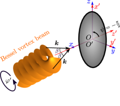
Figure 1: A Bessel vortex beam of $\ell$th-order with half-cone angle $\beta$ interacting with a spheroidal particle. The beam propagates along the $x$ axis toward $-\infty$ and along the $z^{\prime}$ axis toward $+\infty$. The center of both coordinate systems $O(x,y,z)$ (blue axes) and $O^{\prime}(x^{\prime},y^{\prime},z^{\prime})$ (red axes) are located in the particle geometric center. A $90^{\circ}$-counterclockwise rotation around $y$ and $y^{\prime}$ axis maps $O^{\prime}$ onto $O$ system.

III Scattering in the long-wavelength limit

The spheroidal particle has a major and minor axis denoted by $2a$ and $2b$, respectively, with interfocal distance being $d=2\sqrt{a^{2}-b^{2}}$. The acoustic scattering is now described in a coordinate system $O$ fixed in the geometric center of the particle at rest. The major axis lies in the $z$ direction–see Fig. 1. For symmetry reasons, we describe the particle in prolate spheroidal coordinates to which $\xi\geq 1$ is radial distance, $-1\leq\eta\leq 1$, and $0\leq\varphi\leq 2\pi$ is azimuth angle. In this case, the particle corresponds to the surface defined by $\xi=\xi_{0}=2a/d=\text{const.}$ The particle aspect ratio is defined as the major-to-minor axis ratio, which relates to the particle geometric parameter $\xi_{0}$ as

$$\frac{a}{b}=\frac{1}{\sqrt{1-\xi_{0}^{-2}}}.$$ (5)

The particle volume is $V=4\pi ab^{2}/3=\pi d^{3}\xi_{0}(\xi_{0}^{2}-1)/6.$ A spherical particle of radius $r_{0}$ is recovered as $\xi_{0}\rightarrow\infty$, with $\xi_{0}d\rightarrow 2r_{0}$. Whereas a slender particle corresponds to the minor semiaxis being much smaller than the major semiaxis, $a/b\gg 1$ and then $\xi_{0}\approx 1$.

In the long-wavelength scattering analysis, we define the expansion parameter as proportional to the interfocal-to-wavelength ratio as

$$\epsilon=\frac{kd}{2}=\frac{ka}{\xi_{0}}\ll 1.$$ (6)

We emphasize that the other size parameter related to the minor semiaxis $b$, say $kb/\xi_{0}$, is also much smaller than one, as $b<a$. In this case, only the monopole and dipole modes of the incident and scattered waves are needed to describe the particle-wave interaction. Accordingly, the partial wave expansions of the incident and scattering potential velocities in the particle frame are given in prolate spheroidal coordinates by Flammer (2005)

$$\phi_{\text{in}} =\phi_{0}\sum_{n=0}^{1}\sum_{m=-n}^{n}a_{nm}S_{nm}(\epsilon,\eta)R_{nm}^{(1)}(\epsilon,\xi)\textrm{e}^{\textrm{i}m\varphi},$$ (7a)

$$\phi_{\text{sc}} =\phi_{0}\sum_{n=0}^{1}\sum_{m=-n}^{n}a_{nm}s_{nm}S_{nm}(\epsilon,\eta)R_{nm}^{(3)}(\epsilon,\xi)\textrm{e}^{\textrm{i}m\varphi},$$ (7b)

where $S_{nm}$ is the angular function of the first kind, and $R_{nm}^{(1)}$ and $R_{nm}^{(3)}$ are the radial functions of the first and third kind, respectively. The quantities $a_{n}^{m}$ and $s_{nm}$ are the beam-shape and scaled scattering coefficients.

We assume that the particle behaves as a rigid and immovable spheroid. Hence, the velocity normal component is zero on the particle surface, $\partial_{\xi}(\phi_{\textrm{in}}+\phi_{\textrm{sc}})_{\xi=\xi_{0}}=0$. Using (7) in this condition, one obtains the scattering coefficient as

$$s_{nm}=-\frac{\partial_{\xi}R_{nm}^{(1)}}{\partial_{\xi}R_{nm}^{(3)}}\biggr{|}_{\xi=\xi_{0}}.$$ (8)

We shall see in Sec. IV that in the long-wavelength limit, only the dipole scattering coefficients contribute to the acoustic radiation torque. Hence, after Taylor-expanding the radial functions given in (27) around $\epsilon=0$, we obtain the dipole scattering coefficients as Silva and Drinkwater (2018)

$$s_{10} =\frac{\textrm{i}\epsilon^{3}}{6}f_{10}-\frac{\epsilon^{6}}{36}f_{10}^{2},$$ (9a)

$$s_{1,-1} =s_{11}=\frac{\textrm{i}\epsilon^{3}}{12}f_{11}-\frac{\epsilon^{6}}{144}f_{11}^{2},$$ (9b)

where

$$f_{10} =\frac{2}{3}\left[\frac{\xi_{0}}{\xi_{0}^{2}-1}-\ln\left(\frac{\xi_{0}+1}{\sqrt{\xi_{0}^{2}-1}}\right)\right]^{-1},$$ (10a)

$$f_{11} =\frac{8}{3}\left[\frac{2-\xi_{0}^{2}}{\xi_{0}(\xi_{0}^{2}-1)}+\ln\left(\frac{\xi_{0}+1}{\sqrt{\xi_{0}^{2}-1}}\right)\right]^{-1}$$ (10b)

are the scattering factors.

In the far-field $k\xi\gg 1$, the spheroidal expansion in (7) asymptotically approaches the expansion in spherical coordinates $(r,\theta,\varphi)$ as follows Silva and Drinkwater (2018)

$$\phi_{\textrm{in}} =\frac{\phi_{0}}{kr}\sum_{n=0}^{1}\sum_{m=-n}^{n}{a}_{nm}\sin\left(kr-\frac{n\pi}{2}\right)Y_{n}^{m}(\theta,\varphi),$$ (11a)

$$\phi_{\textrm{sc}} =\phi_{0}\frac{\textrm{e}^{\textrm{i}kr}}{kr}\sum_{n=0}^{1}\sum_{m=-n}^{n}\textrm{i}^{-n-1}{a}_{nm}s_{nm}Y_{n}^{m}(\theta,\varphi),$$ (11b)

where $Y_{n}^{m}(\theta,\varphi)$ is the spherical harmonic of $n$th-order and $m$th-degree. Here the beam-shape coefficient $a_{nm}$ describes an incident wave in spherical coordinates. Hereafter, we shall consider the beam-shape coefficients in spherical coordinates.

IV Acoustic radiation torque

The density of linear momentum flux carried by an acoustic wave is well-known from the fluid mechanics theory Silva (2011a) $\overline{\bf{P}}=-\overline{\mathcal{L}}{\bf I}+\rho_{0}\overline{\bm{v}\bm{v}}$, with the over bar denoting time-average over a wave period and $\bf I$ being the unit tensor. The acoustic fields $\mathcal{L}$ and $\rho_{0}\bm{v}\bm{v}$ are the Lagrangian density and Reynolds’ stress tensor. The density of angular momentum flux is then $\overline{\bf{L}}=\bm{r}\times\overline{\bf{P}}$. The radiation force exerted by the incident wave on an surface element $\textrm{d}S$ of the particle is $\textrm{d}\bm{F}_{\text{rad}}=\overline{\bf{P}}\cdot\bm{n}\,\textrm{d}S$, with $\bm{n}$ being the outwardly unit vector at the particle surface $S_{0}$, whereas the moment of the infinitesimal radiation force is given by $\textrm{d}\bm{\tau}_{\text{rad}}=\bm{r}\times\textrm{d}\bm{F}_{\text{rad}}=\overline{\bf{L}}\cdot\bm{n}\,\textrm{d}S$. Therefore, the acoustic radiation torque on the particle is expressed by

$$\bm{\tau}_{\text{rad}}=\int_{S_{0}}\overline{\bf{L}}\cdot\bm{n}\,\textrm{d}S.$$ (12)

As the angular momentum flux satisfies the conservation law Zhang and Marston (2011a) $\nabla\cdot\overline{\bf{L}}=\bm{0}$, the integral can be evaluated over a virtual surface $S_{1}$ of a sphere in the far-field $kr\gg 1$ that encloses the particle. Accordingly, the radiation torque is expressed by $\bm{\tau}_{\text{rad}}=-\int_{S_{1}}\left(\bm{r}\times\rho_{0}\overline{\bm{v}\bm{v}}\right)\cdot\bm{e}_{r}\,\textrm{d}S$, with $\bm{e}_{r}$ being the unit-vector in radial direction. The fluid velocity is the sum of the incident and scattered velocities, $\bm{v}=\bm{v}_{\text{in}}+\bm{v}_{\text{sc}}$. Substituting the total fluid velocity into the far-field expression of the radiation torque and noting that $\overline{\bm{v}\bm{v}}=(1/2)\text{Re}[\bm{v}\bm{v}^{*}]$, we find Lopes et al. (2016)

$$\bm{\tau}_{\text{rad}}=-\frac{\rho_{0}r^{2}}{2}\text{Re}\int_{\Omega_{\text{s}}}\bm{r}\times(\bm{v}_{\text{in}}\bm{v}_{\text{sc}}^{*}+\bm{v}_{\text{sc}}\bm{v}_{\text{in}}^{*}+\bm{v}_{\text{sc}}\bm{v}_{\text{sc}}^{*})\cdot\bm{e}_{r}\,\textrm{d}\Omega_{\text{s}},$$ (13)

where ‘Re’ means the real part of, the asterisk denotes complex conjugation, $\Omega_{\text{s}}$ represents the unit-sphere, and $\textrm{d}\Omega_{\text{s}}$ is solid angle. No torque is formed in the absence of the particle; hence, $\text{Re}\int_{\Omega_{\text{s}}}\bm{r}\times\bm{v}_{\text{in}}\bm{v}_{\text{in}}^{*}\cdot\bm{e}_{r}\,\textrm{d}\Omega_{\text{s}}=\bm{0}$. Using the partial wave expansion in the far-field as given in (11) into Eq. (13), one can show that the Cartesian coordinates of the radiation torque is expressed by Silva et al. (2012)

$${\tau}_{\text{rad},x} =-\frac{E_{0}}{k^{3}\sqrt{2}}\,\text{Re}\biggl{[}(a_{1,-1}+a_{11})(1+s_{11})a^{*}_{10}s^{*}_{10}$$

$$+a_{10}(1+s_{10})(a_{1,-1}^{*}+a_{11}^{*})s_{11}^{*}\biggr{]},$$ (14a)

$${\tau}_{\text{rad},y} =-\frac{E_{0}}{k^{3}\sqrt{2}}\,\text{Re}\biggl{[}\textrm{i}\,(a_{1,-1}-a_{11})(1+s_{11})a^{*}_{10}s^{*}_{10}$$

$$-\textrm{i}\,a_{10}(1+s_{10})(a_{1,-1}^{*}-a_{11}^{*})s_{11}^{*}\biggr{]},$$ (14b)

$${\tau}_{\text{rad},z} =\frac{E_{0}}{k^{3}}\,\text{Re}\left[(|a_{1,-1}|^{2}-|a_{11}|^{2})(1+s_{11})s_{11}^{*}\right].$$ (14c)

Clearly, the radiation torque is caused by the nonlinear interaction between the incident and scattered dipole modes.

To compute the radiation torque from (14), the beam-shape coefficients of the incident wave should be known a priori. Notable examples are plane waves, and Bessel vortex Gong and Marston (2017) and Gaussian beams Mitri and Silva (2014). Numerical schemes and the addition theorem of spherical functions have been employed to compute the coefficients for different types of beam Silva (2011b); Mitri and Silva (2011); Silva et al. (2015, 2013); Lopes et al. (2016).

We now proceed to calculate the FOBB radiation torque in broadside incidence to the particle. In this case, the Bessel beam propagates along the $x$ axis toward $-\infty$ in the particle system $O$. We see in Fig. 1 that the laboratory system $O^{\prime}$ can be mapped onto the particle system $O$ through a $90^{\circ}$-counterclockwise rotation around the $y^{\prime}$ axis.

In the laboratory system $O^{\prime}$, the beam-shape coefficient of the FOBB is given by Mitri and Silva (2011)

$$a^{\prime}_{n\ell}=4\pi\,\textrm{i}^{n-m}Y_{n}^{m}(\beta,0)H(n-m)\delta_{m\ell},$$ (15)

where $H(n-m)$ is the unit-step function, which is equal to $0$ for $n-m<0$ and $1$ for $n-m\geq 0$. According to (14), we have to compute the dipole beam-shape coefficient $a_{1,m}$ in the particle system $O$. The relation between the beam-shape coefficient in the laboratory and particle system is given through the Wigner $D$-function $D_{m\mu}^{n}(\alpha,\psi,\zeta)$ as Mishchenko et al. (2002)

$$a_{nm}=\sum_{\mu=-n}^{n}a^{\prime}_{n\mu}D_{m\mu}^{n}\left(\alpha,\psi,\zeta\right),$$ (16)

where $\alpha$, $\psi,$ and $\zeta$ are the Euler angles. Mapping system $O$ onto $O^{\prime}$ corresponds to the Euler angles $\alpha=0$, $\psi=-\pi/2$, and $\zeta=0$. To obtain $a_{1,m}$ we need only the dipole beam-shape coefficient in system $O^{\prime}$, $a^{\prime}_{1,\mu}$. According to Eq. (16), this coefficient is $a_{1,\mu}^{\prime}=-\delta_{\mu,1}\sqrt{6\pi}\sin\beta.$ By replacing it into Eq. (16), we find the dipole beam-shape coefficients in the particle system as

$$a_{1,-1}=a_{11}=-\sqrt{\frac{3\pi}{2}}\sin\beta,\quad a_{10}=\sqrt{{3\pi}}\sin\beta.$$ (17)

Using this result into (14), we find the radiation torque along the $x$-axis as

$${\tau}_{\text{rad},x}=\frac{3\pi}{k^{3}}E_{0}\sin^{2}\beta\,\text{Re}\left[s_{10}+s_{11}+2s_{10}s_{11}^{*}\right].$$ (18)

Using the scattering coefficients of (9) into this expression, we find

$$\bm{\tau}_{\text{rad}} =-(ka)^{3}\chi\pi a^{3}E_{0}\sin^{2}\beta\,\bm{e}_{x},\quad ka\ll 1,$$ (19a)

$$\chi =\frac{\left(f_{11}-2f_{10}\right)^{2}}{48\xi_{0}^{6}},$$ (19b)

where $\chi$ is related to the difference of the dipole factors.

The asymptotic gyroacoustic expressions as the particle geometric parameter describes a spherical ($\xi_{0}\gg 1$) and slender particle ($\xi_{0}\approx 1$) are given, respectively, by

$$\chi =\frac{3}{400}\left(\frac{1}{\xi_{0}^{4}}-\frac{47}{35\xi_{0}^{6}}\right),$$ (20a)

$$\chi =\frac{4}{27}(\xi_{0}-1)^{2}+{\frac{4}{9}}(\xi_{0}-1)^{3}\left(3+\ln\left[\frac{(\xi_{0}-1)^{2}}{4}\right]\right).$$ (20b)

The radiation torque vanishes as the particle geometry approaches a sphere, $\lim_{\xi_{0}\rightarrow\infty}\tau_{\text{rad}}=0$. This is supported by the fact that no torque is produced on a nonabsorbing sphere Silva et al. (2012).

Importantly, both asymptotic expansions of the gyroacoustic factor in (20) approach to zero. This suggests that the geometric torque factor $\chi$ should have an extreme value in the interval $1\leq\xi_{0}<\infty$. Using the Nelder-Mead numerical method through NMaximize function of Mathematica Software Wolfram Research, Inc. (2019), we find the maximum value $\chi_{\text{max}}=0.14$ at $\xi_{0}=1.3181$.

We now establish the connection between the acoustic radiation torque and acoustic spin. To do so, we express the radiation torque in the laboratory frame (system $O^{\prime}$) as $\bm{\tau}_{\text{rad}}=\gamma\pi a^{3}(ka)^{3}E_{\text{in}}(0)\,\bm{e}_{z^{\prime}}.$ The torque is positive given that $\bm{e}_{z^{\prime}}=-\bm{e}_{x}$, i.e., the $z^{\prime}$ and $x$ axis have opposite orientation. Using Eq. (4), we find at the spin-induced radiation torque on the particle as

$${\tau}_{\text{rad}}=\frac{\chi\pi a^{3}\omega}{2}{S}_{z^{\prime}}(0).$$ (21)

V Particle angular velocity

In broadside incidence, a FOBB may set the spheroidal particle to spin around its minor axis. Here we consider that the particle is immersed in a viscous incompressible fluid with dynamic viscosity $\mu_{0}$. To simplify our analysis, we assume that the yielded flow due to the particle spin has a small Reynolds number $Re\ll 1$, i.e., the so-called Stokes’ flow. It is worth noticing that by solving the acoustic scattering problem we have considered a compressible fluid.

In the laboratory frame (system $O^{\prime}$), the rotation dynamics is described by the Newton’s second law,

$$I_{\text{p}}\dot{\Omega}=\tau_{\text{rad}}-\tau_{\text{drag}}(\Omega),$$ (22)

where $I_{\text{p}}$ is the particle moment of inertia relative to the minor axis, $\Omega$ is the particle angular velocity, and $\tau_{\text{drag}}$ is the drag torque that counteracts the radiation torque.

Assuming the no-slip boundary condition at the particle surface $\xi=\xi_{0}$, one can find the drag torque as Kong et al. (2012)

$$\tau_{\text{drag}}=\pi\mu_{0}d^{3}\tilde{\tau}_{\text{drag}}\,{\Omega},$$ (23a)

$$\tilde{\tau}_{\text{drag}}={\frac{4}{3}\frac{1-2\xi_{0}^{2}}{2\xi_{0}-(1+\xi_{0}^{2})\ln\left(\frac{\xi_{0}+1}{\xi_{0}-1}\right)}.}$$ (23b)

The dimensionless drag torque $\tilde{\tau}_{\text{drag}}$ depends only of the geometry of the particle. As the particle asymptotically approaches ($\xi_{0}\gg 1$) a sphere of radius $r_{0}$, we recover the classical result of the drag torque for a spherical geometry, ${\tau}_{\text{drag}}^{\text{sphere}}=8\pi\mu_{0}r_{0}^{3}\Omega,$ with $r_{0}\approx\xi_{0}d/2$.

Table 1: The acoustic parameters of acoustofluidics and levitation systems at room temperature Lide (2004).

Medium	Density $\rho_{0}\,$\mathrm{[}\mathrm{k}\mathrm{g}\mathrm{/}\mathrm{m}\mathrm{{}^{3}}$]$	Speed of sound $c_{0}\,$\mathrm{[}\mathrm{m}\mathrm{/}\mathrm{s}$]$	Dynamic viscosity $\mu_{0}\,[$\mathrm{Pa}\cdot\mathrm{s}$]$
Air	$1.22$	$343$	$1.86\times 10^{-5}$
Water	$998$	$1483$	$10^{-3}$

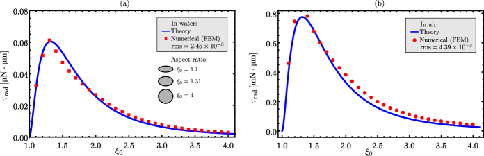
Figure 2: The radiation torque exerted on a particle in (a) water and (b) air as a function of the particle geometric parameter $\xi_{0}$. The torque is evaluated with Eq. (19a) with $\beta=\pi/4$. The parameters for water are $a=120\,\mu$m, $f=1\,$MHz, and $p_{0}=500\,$kPa; while for air, we have $a=680\,\mu$m, $f=40\,$kHz, and $p_{0}=3.5\,$kPa. The red square and circular dots correspond to finite-element simulation results. The maximum value of the radiation torque is at $\xi_{0}=1.31$ ($a/b=1.54$). Three particles with different aspect ratios ($\xi_{0}=1.1,1.31,4$) are depicted in panel (a).

As the angular velocity increases, the radiation and drag torques balance each other. Thus, the particle reaches a stationary angular velocity that can be obtained by combining Eqs. (19a), (22) and (23),

$$\bm{\Omega}_{\text{st}} =\frac{\bm{\tau}_{\text{rad}}}{\pi\mu_{0}d^{3}\tilde{\tau}_{\text{drag}}}=(ka)^{3}\tilde{\Omega}_{\text{st}}\frac{E_{0}}{\mu_{0}}\sin^{2}\beta\,\bm{e}_{z^{\prime}},$$ (24a)

$$\tilde{\Omega}_{\text{st}} =\frac{\chi\xi_{0}^{3}}{{8}\tilde{\tau}_{\text{drag}}},$$ (24b)

with $\tilde{\Omega}_{\text{st}}$ being the dimensionless angular velocity. By measuring the angular velocity $\Omega_{\text{st}}$ and knowing the particle and beam parameters, one can determine the fluid viscosity $\mu_{0}$ through Eq. (24a).

For a quasispherical and slender particle, the dimensionless angular velocity is, respectively,

$$\tilde{\Omega}_{\text{st}} =\frac{3}{3200}\left(\frac{1}{\xi_{0}^{4}}-\frac{31}{70\xi_{0}^{6}}\right),\quad\xi_{0}\gg 1,$$ (25a)

$$\tilde{\Omega}_{\text{st}} =-\frac{1}{36}(\xi_{0}-1)^{2}\left[1+\ln\left(\frac{\xi_{0}-1}{2}\right)\right].\quad\xi_{0}\approx 1.$$ (25b)

The relation between the axial acoustic spin and particle angular velocity follows by replacing Eq. (21) into (24a),

$$\bm{S}_{z^{\prime}}(0) =\gamma\bm{\Omega}_{\text{st}}$$ (26a)

$$\gamma =\frac{16\mu_{0}\tilde{\tau}_{\text{drag}}}{(ka)^{3}\chi\xi_{0}^{3}\omega},$$ (26b)

where $\gamma$ is the gyroacoustic ratio of the spin and angular velocity in the SI units of $\mathrm{kg}\text{\,}{\mathrm{m}}^{-1}$. This result describes how the spin is transferred to a subwavelength spheroidal particle. It also enables the experimental assessment of the acoustic spin by measuring the angular velocity of a subwavelength spheroidal particle.

VI Model predictions

We provide some predictions for typical experimental setups of acoustical vortex tweezers Baudoin et al. (2019) and acoustic levitation Marzo et al. (2015) to which the particle is immersed in a water-like medium and air, respectively. The acoustic parameters of these fluids are summarized in Table 1. The particle has a fixed major semiaxis of $a=$680\text{\,}\mathrm{\SIUnitSymbolMicro m}$$ in air and $a=$120\text{\,}\mathrm{\SIUnitSymbolMicro m}$$ in water.

The theoretical predictions will be compared with 3D finite-element simulation results performed in Comsol Multiphysics (Comsol Inc., USA). The radiation torque was computed by numerical integration of the angular momentum flux $\overline{\bf{L}}$ over the particle surface as described in Eq. (12). The mean discretization length on the surface is $b/50$; while in the surrounding fluid, we consider at least $\lambda/12$. The domain has a cylindrical geometry with $36b$ diameter and height. We have also adopted the first-order scattering boundary condition at the domain edges.

In Fig. 2, we show the radiation torque exerted on a spheroidal particle as a function of the geometric parameter $\xi_{0}$ in water and air. The torque is evaluated with Eq. (19a). The pressure peaks are $p_{0}=$3.5\text{\,}\mathrm{kPa}$$ (air) and $p_{0}=$0.5\text{\,}\mathrm{MPa}$$ (water). The driving frequencies are $f=$40\text{\,}\mathrm{kHz}$$ (air) and $f=$1\text{\,}\mathrm{MHz}$$ (water). The half-cone angle of the beam is $\beta=\pi/4$. According to Eq. (6) the size parameter $\epsilon$ is always smaller than $0.51$. The radiation torques peak at $\xi_{0}=1.31$, which corresponds to the aspect ratio $a/b=1.54$. finite-element results are also depicted for comparison. The root mean square error (rms) is about $10^{-3}$ in both cases.

In Fig. 3, we plot the angular velocity versus the particle geometric parameter $\xi_{0}$ with different peak pressures $p_{0}=1,\,$2\text{\,}\mathrm{kPa}$$ (air) and $p_{0}=100,\,$500\text{\,}\mathrm{kPa}$$ (water). We note that the peak velocity is reached at $\xi_{0}=1.21$, which corresponds to the aspect ratio $a/b=1.77$. When compared to the radiation torque, this maximum value appears for a different geometric parameter. This happens because the viscous drag torque acts on the particle, as shown in Eq. (24b), changing the optimal aspect ratio for the angular velocity. In water, the angular velocity can be as large as $100$ rpm, whereas in air, it can be ten times this value.

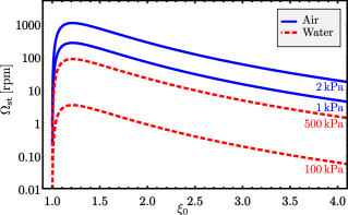
Figure 3: The stationary angular velocity as a function of the particle geometric parameter $\xi_{0}$ for different peak pressures in water and air. The velocity is calculated with Eq. (24a) and $\beta=\pi/4$. The parameters for water are $a=120\,\mu$m and $f=1\,$MHz; and for air, $a=680\,\mu$m and $f=40\,$kHz. The maximum value of the angular velocity is at $\xi_{0}=1.21$ ($a/b=1.77$).

VII Summary and conclusion

We have demonstrated that the acoustic spin can be transferred to a subwavelength spheroidal particle. Using the partial wave expansion of the incident and scattered velocity potentials in spheroidal coordinates and integrating the total angular momentum density in the far-field, we derived a general expression of the radiation torque in the long-wavelength limit. Considering a broadside incidence of a FOBB onto the particle centered at the beam axis, we obtained the corresponding radiation torque. In turn, the torque produces an angular velocity on the particle that rotates around its minor axis.

We offer a more fundamental explanation of the spin-induced torque using a description from quantum physics. The acoustic FOBB is regarded as a spin-1 field Bliokh and Nori (2019), whereas a prolate spheroid can be classified as a spin-0 and spin-1 particle under axial and transverse rotations, respectively. Therefore, we found that the spin can only be transferred from the FOBB in broadside incidence to the particle inducing a transverse rotation. Importantly, axial rotations can be generated by viscous torques caused by tangential stresses within the particle boundary layer. However, the viscous torque can be neglected as the boundary layer thickness, $\delta=(2\mu_{0}/\rho_{0}\omega)^{1/2}$ is much smaller than the particle size Lee and Wang (1989). Here $\delta/a\sim 10^{-3}$ (in water) and $\delta/a\sim 10^{-2}$ (in air). For this reason, this torque was discarded in our analysis.

The stationary angular velocity is obtained by taking the radiation and drag torque balance in Eq. (22). Considering the physical parameters of acoustofluidic and experimental levitation setups, our model predicts that the stationary angular velocity can reach $100\text{\,}\,\mathrm{r}\mathrm{p}\mathrm{m}$ in water and $1000\text{\,}\,\mathrm{r}\mathrm{p}\mathrm{m}$ in air. Therefore, it is feasible to measure the angular velocity and use the result to obtain the acoustic spin. We can also determine the fluid viscosity by measuring the angular velocity. Additionally, by measuring the acoustic spin, we can obtain the beam energy density as described in Eq. (2). This may provide a means of assessing the energy of focused ultrasonic vortices in acoustic levitation systems Marzo et al. (2015) and acoustical vortex tweezers Baudoin et al. (2019).

In conclusion, we have established a connection between the acoustic spin and the angular velocity of a spheroidal particle in a viscous fluid. The developed method can also be applied to unveil the properties of other spin-carrying acoustic beams.

Appendix A Monopole and dipole radial functions

In the long-wavelength limit, the radial spheroidal functions are given to the $\epsilon^{6}$-order by Burke (1966)

$$R_{00}^{(1)} =1+\frac{\epsilon^{2}}{18}\left(2-3C_{1}^{2}\right)+\frac{\epsilon^{4}}{16200}\biggl{[}112-180C_{1}^{2}+135C_{1}^{4}+\frac{\epsilon^{2}}{882}\left(2192-8064C_{1}^{2}+5670C_{1}^{4}-2835C_{1}^{6}\right)\biggr{]},$$ (27a)

$$R_{10}^{(1)} =\frac{\epsilon}{C_{1}}+\frac{\epsilon^{2}C_{1}}{150}\biggl{[}2-5C_{1}^{2}+\frac{\epsilon^{2}}{4900}\left(368-700C_{1}^{2}+875C_{1}^{4}\right)\biggr{]},$$ (27b)

$$R_{11}^{(1)} =\frac{\epsilon S_{1}}{3}+\frac{\epsilon^{3}S_{1}}{150}\biggl{[}4-5C_{1}^{2}+\frac{\epsilon^{2}}{4900}(712-1400C_{1}^{2}+875C_{1}^{4})\biggr{]},$$ (27c)

$$R_{00}^{(2)} =-\frac{2}{\epsilon}\biggl{\{}L-\frac{\epsilon^{2}}{6}[6C_{1}+L(3C_{2}-5)]+\frac{3}{5}\left(\frac{\epsilon}{6}\right)^{4}\left[11C_{1}+9C_{3}+\frac{L}{60}(1109-1380C_{2}+135C_{4})\right]\biggr{\}},$$ (27d)

$$R_{10}^{(2)} =\frac{3C_{1}}{\epsilon^{2}}\biggl{\{}2C_{1}-\frac{C_{2}}{C_{1}}-2L-\left(\frac{\epsilon}{10}\right)^{2}\left[18C_{1}-\frac{4C_{2}}{C_{1}}+L(22-10C_{2})\right]+\frac{1}{882}\left(\frac{\epsilon}{10}\right)^{4}$$

$$\times\biggl{[}272313C1-864\frac{C_{2}}{C_{1}}+7875C_{3}-L(116073-99540C_{2}+7875C_{2})\biggr{]}\biggr{\}},$$ (27e)

$$R_{11}^{(2)} =-\frac{3S_{1}}{2\epsilon^{2}}\biggl{\{}\frac{C_{1}}{S_{1}^{2}}-2L-\left(\frac{\epsilon}{10}\right)^{4}\biggl{[}8C_{1}\left(5-\frac{1}{S_{1}^{2}}\right)-8L(33+5C_{2})\biggr{]}-\frac{1}{196}\left(\frac{\epsilon}{10}\right)^{2}\biggl{[}85800C_{1}-1750C_{3}$$

$$+\frac{712C_{1}}{S_{1}^{2}}-L(106324-76950C_{2}-1750C_{4})\biggr{]}\biggr{\}},$$ (27f)

$$R_{nm}^{(3)} =R_{nm}^{(1)}+\textrm{i}R_{nm}^{(2)},$$ (27g)

where $R_{nm}^{(2)}$ is the radial function of the second-kind. Note that $R_{nm}^{(i)}=R^{(i)}_{n,-m}$, with $i=1,2,3$. The auxiliary functions are expressed by

$$C_{n} =\frac{1}{2}\left[(\sqrt{\xi^{2}-1}+\xi)^{n}+(\sqrt{\xi^{2}-1}+\xi)^{-n}\right],$$

$$S_{n} =\frac{1}{2}\left[(\sqrt{\xi^{2}-1}+\xi)^{n}-(\sqrt{\xi^{2}-1}+\xi)^{-n}\right],$$

$$L =\frac{1}{2}\ln\left(\frac{1+(\sqrt{\xi^{2}-1}+\xi)^{-1}}{1-(\sqrt{\xi^{2}-1}+\xi)^{-1}}\right).$$

Appendix B Wigner $D$ function

The Wigner $D$ function $D_{\mu m}^{n}(0,-\pi/2,0)$ was evaluated with Mathematica Software (Wolfram Inc., USA). To the dipole approximation, we have

$$D_{00}^{0}=1,$$ (28a)

$$D_{-1,-1}^{1}=D_{-1,1}^{1}=D_{1,-1}^{1}=D_{11}^{1}=\frac{1}{2},$$ (28b)

$$D_{-1,0}^{1}=D_{01}^{1}=-\frac{1}{\sqrt{2}},$$ (28c)

$$D_{0,-1}^{1}=D_{10}^{1}=\frac{1}{\sqrt{2}},$$ (28d)

$$D_{00}^{1}=0.$$ (28e)

References

- Ohanian (1986) H. C. Ohanian, Am. J. Phys. 54, 500 (1986).
- Belinfante (1939) F. J. Belinfante, Physica 6, 887 (1939).
- Shi et al. (2019) C. Shi, R. Zhao, Y. Long, S. Yang, Y. Wang, H. Chen, J. Ren, and X. Zhang, Nat. Sci. Rev. 6, 707 (2019).
- Bliokh and Nori (2019) K. Y. Bliokh and F. Nori, Phys. Rev. B 99, 174310 (2019).
- Silva (2014) G. T. Silva, J. Acoust. Soc. Am. 136, 2405 (2014).
- Zhang and Marston (2011a) L. Zhang and P. L. Marston, J. Acoust. Soc. Am. 129, 1679 (2011a).
- Zhang and Marston (2011b) L. Zhang and P. L. Marston, Phys. Rev. E 84, 065601 (2011b).
- Silva et al. (2012) G. T. Silva, T. P. Lobo, and F. G. Mitri, Europhys. Lett. 97, 54003 (2012).
- Mitri et al. (2012) F. G. Mitri, T. P. Lobo, and G. T. Silva, Phys. Rev. E 85, 026602 (2012).
- Zhang and Marston (2013) L. Zhang and P. L. Marston, Biomed. Opt. Expr. 4, 1610 (2013).
- Mitri (2016) F. G. Mitri, Ultrasonics 72, 57 (2016).
- Zhang (2018) L. Zhang, Phys. Rev. Applied 10, 034039 (2018).
- Gong et al. (2019) Z. Gong, P. L. Marston, and W. Li, Phys. Rev. Appl. 11, 064022 (2019).
- Schwarz et al. (2015) T. Schwarz, P. Hahn, G. Petit-Pierre, and J. Dual, Microfluid Nanofluid 18, 65 (2015).
- Wang et al. (2012) W. Wang, L. A. Castro, M. Hoyos, and T. E. Mallouk, ACS Nano 67, 6122 (2012).
- Wijaya and Lim (2015) F. B. Wijaya and K.-M. Lim, Acta Acust. united Ac. 101, 531 (2015).
- Jerome et al. (2019) T. S. Jerome, Y. A. Ilinskii, E. A. Zabolotskaya, and M. F. Hamilton, J. Acoust. Soc. Am. 145, 36 (2019).
- Fan et al. (2008) Z. Fan, D. Mei, K. Yang, and Z. Chen, J. Acoust. Soc. Am. 124, 2727 (2008).
- Silva et al. (2013) G. T. Silva, J. H. Lopes, and F. G. Mitri, IEEE Trans. Ultrason. Ferroelectr. Freq. Control 60, 1207 (2013).
- Zhang and Marston (2011c) L. Zhang and P. L. Marston, Phys. Rev. E 84, 035601 (2011c).
- Leão-Neto and Silva (2016) J. P. Leão-Neto and G. T. Silva, Ultrasonics 71, 1 (2016).
- Kong et al. (2012) D. Kong, Z. Cui, Y. Pan, and K. Zhang, Intl. J. Pure Appl. Math. 75, 455 (2012).
- Marzo et al. (2015) A. Marzo, S. A. Seah, B. W. Drinkwater, D. R. Sahoo, B. Long, and S. Subramanian, Nat. Commun. 6, 8661 (2015).
- Baudoin et al. (2019) M. Baudoin, J.-C. Gerbedoen, A. Riaud, O. B. Matar, N. Smagin, and J.-L. Thomas, Sci. Adv. 5, eaav1967 (2019).
- Flammer (2005) C. Flammer, Spheroidal Wave Functions (Dover Publications, London, 2005).
- Silva and Drinkwater (2018) G. T. Silva and B. W. Drinkwater, J. Acoustic. Soc. Am. 144, EL453 (2018).
- Silva (2011a) G. T. Silva, J. Acoust. Soc. Am. 130, 3541 (2011a).
- Lopes et al. (2016) J. H. Lopes, M. Azarpeyvand, and G. T. Silva, IEEE Trans. Ultrason. Ferroelectr. Freq. Control 63, 186 (2016).
- Gong and Marston (2017) Z. Gong and P. L. Marston, J. Acoust. Soc. Am. 141, EL574 (2017).
- Mitri and Silva (2014) F. G. Mitri and G. T. Silva, Phys. Rev. E 90, 053204 (2014).
- Silva (2011b) G. T. Silva, IEEE Trans. Ultrason. Ferroelectr. Freq. Control 58, 298 (2011b).
- Mitri and Silva (2011) F. G. Mitri and G. T. Silva, Wave Motion 46, 392 (2011).
- Silva et al. (2015) G. T. Silva, A. L. Baggio, J. H. Lopes, and F. G. Mitri, IEEE Trans. Ultrason. Ferroelectr. Freq. Control 62, 576 (2015).
- Mishchenko et al. (2002) M. I. Mishchenko, L. D. Travis, and A. A. Lacis, Scattering, Absorption, and Emission of Light by Small Particles (Cambridge University Press, Cambridge, 2002).
- Wolfram Research, Inc. (2019) Wolfram Research, Inc., “Mathematica, Version 10.0,” https://www.wolfram.com/mathematica (2019), Champaign, IL.
- Lide (2004) D. R. Lide, CRC Handbook of Chemistry and Physics, 84th ed. (CRC Press, Boca Raton, FL, 2004).
- Lee and Wang (1989) C. P. Lee and T. G. Wang, J. Acoust. Soc. Am. 85, 1081 (1989).
- Burke (1966) J. E. Burke, Stud. Appl. Math. 45, 425 (1966).