CNN-based Density Estimation and Crowd Counting: A Survey

Abstract

Accurately estimating the number of objects in a single image is a challenging yet meaningful task and has been applied in many applications such as urban planning and public safety. In the various object counting tasks, crowd counting is particularly prominent due to its specific significance to social security and development. Fortunately, the development of the techniques for crowd counting can be generalized to other related fields such as vehicle counting and environment survey, if without taking their characteristics into account. Therefore, many researchers are devoting to crowd counting, and many excellent works of literature and works have spurted out. In these works, they are must be helpful for the development of crowd counting. However, the question we should consider is why they are effective for this task. Limited by the cost of time and energy, we cannot analyze all the algorithms. In this paper, we have surveyed over 220 works to comprehensively and systematically study the crowd counting models, mainly CNN-based density map estimation methods. Finally, according to the evaluation metrics, we select the top three performers on their crowd counting datasets and analyze their merits and drawbacks. Through our analysis, we expect to make reasonable inference and prediction for the future development of crowd counting, and meanwhile, it can also provide feasible solutions for the problem of object counting in other fields. We provide the density maps and prediction results of some mainstream algorithm in the validation set of NWPU dataset for comparison and testing. Meanwhile, density map generation and evaluation tools are also provided. All the codes and evaluation results are made publicly available at https://github.com/gaoguangshuai/survey-for-crowd-counting.

I Introduction

Over the past few decades, an increasing number of research communities, have considered the problem of object counting as their mainly research direction, as a consequence, many works have been published to count the number of objects in images or videos across wide variety of domains such as crowding counting [1, 2, 3, 4, 5, 6, 7, 8, 9, 10, 11, 12, 13], cell microscopy [14, 15, 16], animals [17], vehicles [2, 18, 19, 20], leaves [21, 22] and environment survey [23, 24]. In all these domains, crowd counting is of paramount importance, and it is crucial to building a more high-level cognitive ability in some crowd scenarios, such as crowd analysis [25, 26] and video surveillance [27]. As the increasing growth of the world’s population and subsequent urbanization result in a rapid crowd gathering in many scenarios such as parades, concerts and stadiums. In these scenarios, crowd counting plays an indispensable role for social safety and control management.

Considering the specific importance of crowd counting aforementioned, more and more researchers have attempted to design various sophisticated projects to address the problem of crowd counting. Especially in the last half decades, with the advent of deep learning, Convolution Neural Networks (CNNs) based models have been overwhelmingly dominated in various computer vision tasks, including crowd counting. Although different tasks have their unique attributes, there exist common features such as structural features and distribution patterns. Fortunately, the techniques for crowd counting can be extended to some other fields with specific tools. Therefore, in this paper, we expect to provide a reasonable solution for other tasks through the deep excavation of the crowd counting task, especially for CNN-based density estimation and crowd counting models. Our survey aims to involve various parts, which is ranging algorithm taxonomy from some interesting under-explored research direction. Beyond taxonomically reviewing existing CNN-based crowd counting and density estimation models, representing datasets and evaluation metrics, some factors and attributes, which largely affect the performance the designed model, are also investigated, such as distractors and negative samples. We provide the density maps and prediction results of some mainstream algorithm in the validation set of NWPU dataset [28] for comparison and testing. Meanwhile, density map generation and evaluation tools are also provided. All the codes and evaluation results are made publicly available at https://github.com/gaoguangshuai/survey-for-crowd-counting.

I-A Related Works and Scope

The various approaches for crowd counting are mainly divided into four categories: detection-based, regression-based, density estimation, and more recently CNN-based density estimation approaches. We focus on the CNN-based density estimation and crowd counting model in this survey. For the sake of completeness, it is necessary to review some other related works in this subsection.

Early works [29, 30, 31, 32] on crowd counting use detection-based approaches. These approaches usually apply a person or head detector via a sliding window on an image. Recently many extraordinary object detectors such as R-CNN [33, 34, 35], YOLO [36], and SSD [37] have been presented, which may perform dramatic detection accuracy in the sparse scenes. However, they will present unsatisfactory results when encountered the situation of occlusion and background clutter in extremely dense crowds.

To reduce the above problems, some works [38, 27, 39] introduce regression-based methods which directly learn the mapping from an image patch to the count. They usually first extract global features [40] (texture, gradient, edge features), or local features [41] (SIFT [42], LBP [43], HOG [44], GLCM [45]). Then some regression techniques such as linear regression [46] and Gaussian mixture regression [47] are used to learn a mapping function to the crowd counting.

These methods are successful in dealing with the problems of occlusion and background clutter, but they always ignore spatial information. Therefore, Lemptisky et al. [16] first adopt a density estimation based method by learning a linear mapping between local features and corresponding density maps. For reducing the difficulty of learning a linear mapping, [48] proposes a non-linear mapping, random forest regression, which obtains satisfactory performance by introducing a crowdedness prior and using it to train two different forests. Besides, this method needs less memory to store the forest. These methods consider the spatial information, but they only use traditional hand-crafted features to extract low-level information, which cannot guide the high-quality density map to estimate more accurate counting.

Recently, benefiting from the powerful feature representation of CNNs, more researchers utilize it to improve the density estimation. Earlier heuristic models typically leverage basic CNNs to predict the density of the crowds [49, 50, 51, 15], which obtain significant improvement compared with traditional hand-crafted features. Lately, more effective and efficient models based on Fully Convolution Network (FCN), which has become the mainstream network architecture for the density estimation and crowd counting. Different supervised level and learning paradigm for different models, also there are some models designed in cross scene and multiple domains. A brief chronology is shown in Fig. 1, which illustrates the main advancements and milestones of crowd counting techniques. The goal of this survey is focused on the modern CNN-based for density estimation and crowd counting, Fig. 2 depicts a taxonomy of curial methodologies to be covered in the survey.

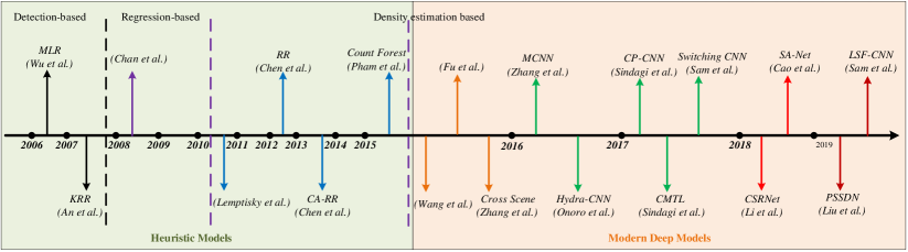
Figure 1: A brief chronology of crowd counting. The first incorporation of deep learning techniques for crowd counting is from 2015. See Section 1 for more detailed description. Milestone models in this figure: MLR [52], KRR [53], Chan et al. [27], Lemptisky et al. [16], RR [40], CA-RR [54], Count Forest [48], Wang et al. [49], Fu et al. [50], Cross scene [51], MCNN [1], Hydra-CNN [2], CP-CNN [6], CMTL [55], switching CNN [5], CSRNet [12], SANet [11], PSSDN [56] and LSF-CNN [57]. The trend in the past few years has been designing crowd counting models based on multi-column (in green), single-column (in red) network architecture and object localization or tracking depending on counting techniques (in crimson), which are either contemporary and potential direction in future. While traditional heuristic methods are highlighted with the blue-shaded area and the modern CNN-based density estimation and crowd counting models are with the red-shaded backgrounds, respectively.

Scope of the survey. Considering that reviewing all state-of-the-art methods is impractical (and fortunately unnecessary), this paper sorts out some mainstream algorithms, which are all influential or essential papers published in, but not limited to, prestigious journals and conferences. The survey focuses on the modern CNN-based density estimation methods in recent years, and some early works are also included for the sake of completeness. We classify existing methods into several categories, in terms of network architecture, supervision form, influence of cross-scene or multi-domain, etc. Such comprehensive and systematic taxonomies can be more helpful for the readers to in-depth understand the progress of crowd counting in the past years.

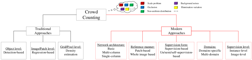
Figure 2: The overall architecture of this work. We concentrate on the modern density map-based approaches mainly CNN-based for crowd counting.

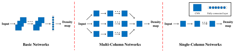
Figure 3: Comparison of the structure of existing density map-based networks.

I-B Related previous reviews and surveys

TABLE I: Summary of previous reviews.

#	Title	Year	Venue	Brief description
1	Crowd analysis: a survey [24]	2008	MVA	This paper presents a survey on crowd analysis methods employed in computer vision research and discusses perspectives from other research disciplines and how they can contribute to the computer vision approach.
2	Crowd analysis using computer vision techniques [58]	2010	ISPM	A survey on crowd analysis by using computer vision techniques, including different aspects such as people tracking, crowd density estimation, event detection, validation and simulation.
3	A Survey of Human-Sensing:Methods for Detecting Presence, Count, Location, Track, and Identity [59]	2010	ACM Computing Surveys	a survey of the inherently multidisciplinary literature of human-sensing , focusing mainly on the extraction of five commonly needed spatio-temporal properties: namely presence, count, location, track and identity.
4	Crowd counting and profiling: Methodology and evaluation [60]	2013	MSVAC	This study describes and compares the state-of-the-art methods for video imagery based crowd counting, and provides a systematic evaluation of different methods using the same protocol.
5	Performance evaluation of crowd image analysis using the PETS2009 dataset [61]	2014	PRL	This paper presents PETS2009 crowd analysis dataset and highlights detection and tracking performance on it
6	Crowded scene analysis: A survey [62]	2015	TCSVT	This paper surveys the state-of-the-art techniques on crowded scene analysis with different methods such as crowd motion pattern learning, crowd behavior, activity analysis and anomaly detection in crowds.
7	An evaluation of crowd counting methods, features and regression models [63]	2015	CVIU	This paper presents an evaluation across multiple datasets to compare holistic, local and histogram based methods, and to compare various image features and regression models.
8	Recent survey on crowd density estimation and counting for visual surveillance [64]	2015	EAAI	This paper presents a survey on crowd density estimation and counting methods employed for visual surveillance in the perspective of computer vision research.
9	Advances and trends in visual crowd analysis: A systematic survey and evaluation of crowd modelling techniques [65]	2016	Neurocomputing	This paper aims to give an account of such issues by deducing key statistical evidence from the existing literature and providing recommendations towards focusing on the general aspects of techniques rather than any specific algorithm.
10	Crowd scene understanding from video: a survey [66]	2017	TOMM	This survey explores crowd analysis as it relates to two primary research areas: crowd statistics and behavior understanding.
11	A survey of recent advances in cnn-based single image crowd counting and density estimation [67]	2018	PRL	A review of various single image crowd counting and density estimation methods with a specific focus on recent CNN-based approaches.
12	Convolutional neural networks for crowd behaviour analysis: a survey [68]	2019	VC	A survey for crowd analysis using CNN

Table I lists the existing reviews or surveys which are related to our paper. Notably, Zhan et al [24] and Junior et al. [58] are the first ones for crowd analysis. Li et al. [62] review the task of crowded scene analysis with different methods, while Zitouni et al. [65] evaluate different methods with different criteria. Loy et al. [60] make detailed comparisons of state-of-the-arts for crowd counting based on video imagery with the same protocol. Ryan et al. [60] present an evaluation across multiple datasets to compare various image features and regression models and Saleh et al. [64] survey two main approaches in direct and indirect manners. Grant et al. [66] explore two kinds of crowd analysis. While these surveys make detail analysis on crowd counting and scene analysis, they are only for traditional methods with hand-crafted features. In recent work, Sindagi et al. [67] provide a survey of recent state-of-the-art CNN-based approaches for crowd counting and density estimation for the single image. However, it only roughly introduces the latest advancement of CNN-based methods, which are only up to the year 2017. Tripathi et al. [68] put forward a review on crowd analysis using CNN, which is not just for crowd counting, thereby it was not adequate comprehensive and in-depth. As we know, the techniques are incremental month by month, and it is also an urgent need for us to document the development of crowd counting in the past half-decade.

Different from previous surveys that focus on hand-crafted features or primitive CNNs, our work systematically and comprehensively reviews CNN-based density estimation crowd counting approaches. Specifically, we summarize the existing crowd counting models from various aspects and list the results of some representing mainstream algorithms in terms of evaluation metrics on several typical benchmark crowd counting datasets. Finally, we select the top three performers and carefully and thoroughly analyze the properties of these models. We also offer insights for essential open issues, challenges, and future direction. Through this survey, we expect to make reasonable inference and prediction for the future development of crowd counting, and meanwhile, it can also provide feasible solutions and make guidance for the problem of object counting in other domains.

I-C Contributions of this paper

In summary, the contributions in this paper are mainly in the following folds:

1. Comprehensive and systematic overview from various aspects. We category the CNN-based models according to several taxonomies, including network architecture, supervised form, learning paradigm, etc. The taxonomies can motivate researches with a deep understanding of the critical techniques of CNN-based methods.

2. Attribute-based performance analysis. Based on the performance of the SOTA methods, we analyze the reasons why they perform well, the techniques they utilize. Besides, we discuss the various challenge factors that promote researchers to design more effective algorithms.

3. Open questions and future directions. We look through some important issues for model design, dataset collection, and some generalization to other domains with domain adaptation or transfer learning and explore some promising research directions in the future.

These contributions provide detailed and in-depth review, which differs from the previous review or survey works to a large extent.

The remainder of the paper is organized as follows. Section II conducts a comprehensive literature review of mainstream CNN-based density estimation and crowd counting models according to the proposed taxonomies. Section III examines the most notable datasets for crowd counting and some datasets for other object counting tasks, while section IV describes several widely used evaluation metrics. Section V benchmarks some representing models and makes an in-depth analysis. Section VI presents a discussion and put forward some open issues and possible future directions. Finally, the conclusion is concluded in Section VII.

TABLE II: Summary of state-of-the-art methods. See II for more detailed description.

Methods	Year$\&$Venue	Network architecture	Reference manner	Supervision form	Learning paradigm	Supervision level
Fu et al. [50]	2015 EAAI	Basic	Patch-based	Fully-Sup.	STL	Instance level
Wang et al. [49]	2015 ACMMM	Basic	Patch-based	Fully-Sup.	STL	Instance level
Cross scene [51]	2015 CVPR	Basic	Patch-based	Fully-Sup.	MTL	Instance level
MCNN [1]	2016 CVPR	Multi-column	Whole image-based	Fully-Sup.	STL	Instance level
Crowdnet [3]	2016 ACMMM	Multi-column	Patch-based	Fully-Sup.	STL	Instance level
CNN-Boosting [15]	2016 ECCV	Basic	Patch-based	Fully-Sup.	STL	Instance level
Hydra-CNN [2]	2016 ECCV	Multi-column	Patch-based	Fully-Sup.	MTL	Instance level
Shang et al. [69]	2016 ECCV	Multi-column	Whole image-based	Fully-Sup.	STL	Instance level
CMTL [55]	2017 AVSS	Multi-column	Whole image-based	Fully-Sup.	MTL	Instance level
Switching CNN [5]	2017 CVPR	Multi-column	Patch-based	Fully-Sup.	MTL	Instance level
CP-CNN [6]	2017 ICCV	Multi-column	Whole image-based	Fully-Sup.	MTL	Instance level
D-ConvNet [70]	2018 CVPR	Single-column	Whole image-based	Filly-Sup.	STL	Instance level
CSRNet [12]	2018 CVPR	Single-column	Whole image-based	Fully-Sup.	STL	Instance level
DRSAN [71]	2018 IJCAI	Multi-column	Whole image-based	Fully-Sup.	STL	Instance level
DecideNet [7]	2018 CVPR	Multi-column	Patch-based	Fully-Sup.	MTL	Instance level
SaCNN [9]	2018 WACV	Single column	Whole image-based	Fully-Sup.	MTL	Instance level
SACNN [11]	2018 ECCV	Single column	Patch-based	Fully-Sup.	MTL	Instance level
IG-CNN [72]	2018 CVPR	Multi-column	Patch-based	Fully-Sup.	MTL	Instance level
ic-CNN [73]	2018 ECCV	Multi-column	Whole image-based	Fully-Sup.	MTL	Instance level
ACSCP [74]	2018 CVPR	Multi-column	Patch-based	Fully-Sup.	MTL	Instance level
NetVLAD [75]	2018 TII	Single-column	Whole image-based	Fully-Sup.	MTL	Instance level
CL [76]	2018 ECCV	Single-column	Patch-based	Fully-Sup.	MTL	Instance level
L2R [77]	2018 CVPR	Basic	Whole image-based	Self-Sup.	MTL	–
GAN-MTR [78]	2018 WACV	Basic	Whole image-based	Semi-Sup.	MTL	–
PaDNet [79]	2019 TIP	Single-column	Patch-based	Fully-Sup.	STL	Instance level
ASD [80]	2019 ICASSP	Multi-column	Whole image-based	Fully-Sup.	MTL	Instance level
SPN [81]	2019 WACV	Single column	Whole image-based	Fully-Sup.	STL	Instance level
SR-GAN [82]	2019 CVIU	Basic	Whole image-based	Semi-Sup.	MTL	–
ADCrowdnet [83]	2019 CVPR	Single column	Whole image-based	Fully-Sup.	STL	Instance level
SAAN [8]	2019 WACV	Multi-column	Whole image-based	Fully-Sup.	MTL	Instance level
SAA-Net [13]	2019 CVPR	Single column	Whole image-based	Fully-Sup.	MTL	Instance level
SFCN${\dagger}^{2}$ [84]	2019 CVPR	Single column	Whole image-based	Fully-Sup.	STL	Instance level
SE Cycle GAN [84]	2019 CVPR	Single column	Whole image-based	Fully-Sup.	STL	Instance level
PACNN [85]	2019 CVPR	Single column	Whole image-based	Fully-Sup.	STL	Instance level
CAN&ECAN [86]	2019 CVPR	Single column	Whole image-based	Fully-Sup.	STL	Instance level
CFF [87]	2019 ICCV	Single-column	Whole image-based	Fully-Sup.	MTL	Instance level
PCC Net [88]	2019 TCSVT	Multi-column	Whole image-based	Fully-Sup.	MTL	Instance level
SFANet [89]	2019 CVPR	Single column	Whole image-based	Fully-Sup.	MTL	Instance level
W-Net [90]	2019 CVPR	Single column	Whole image-based	Fully-Sup.	STL	Instance level
SL2R [91]	2019 CVPR	Basic	Whole image-based	Self-Sup.	MTL	–
TEDnet [92]	2019 CVPR	Single column	Whole image-based	Fully-Sup.	STL	Instance level
RReg [93]	2019 CVPR	Multi-column	Whole image-based	Fully-Sup.	STL	Instance level
RAZNet [94]	2019 CVPR	Multi-column	Whole image-based	Fully-Sup.	MTL	Instance level
AT-CNN [95]	2019 CVPR	Single-column	Whole image-based	Fully-Sup.	MTL	Instance level
GWTA-CCNN [96]	2019 AAAI	Single column	Patch-based	Un-Sup.	STL	–
HA-CCN [97]	2019 TIP	Single column	Whole image-based	Fully-Sup./Weak-Sup	STL	Instance/Image level
L2SM [98]	2019 ICCV	Single column	Patch-based	Fully-Sup	STL	Instance level
RANet [99]	2019 ICCV	Multi-column	Whole image-based	Fully-Sup	STL	Instance level
McML [100]	2019 ACM MM	Multi-column	Whole image-based	Fully-Sup	STL	Instance level
ILC [101]	2019 CVPR	Multi-column	Whole image-based	Fully-Sup.	MTL	Image level

II Taxonomy for crowd counting

In this section, we review CNN-based crowd counting algorithms in the following taxonomies. Chiefly is representative network architectures for crowd counting (II-A). Next is the learning paradigm of the methods (II-B), and then is the inference manner of the networks (II-C). Additionally, the supervision forms of networks are also introduced in II-D. Meanwhile, to evaluate the generalization ability of the algorithms, we classify existing works into domain-specific and multi-domain ones (II-E). Finally, based on the supervised level, we classify the CNN-based models into instance-level and image-level ones (II-F). We group the important models and describe them roughly in chronological order. A summary of the state-of-the-art is presented in Table II.

II-A Representative network architectures for crowd counting

In view of different types of network architectures, we divide crowd counting models into three categories: basic CNN based methods, multi-column based methods, and single-column based methods. The category of network architectures is illustrated in Fig. 3.

II-A1 Basic CNN

This network architecture adopts the basic CNN layers which convolutional layers, pooling layers, uniquely fully connected layers, without additional feature information required. They generally are involved in the initial works using CNN for density estimation and crowd counting.

$\bullet$ Fu et al. [50] put forward the first CNN-based model for crowd counting, which accelerates the speed and accuracy of the model by removing some similar network connections existed in feature maps and cascading two ConvNet classifiers.

$\bullet$ Wang et al. [49] propose a deep network based on Alexnet architecture [102] for extremely dense crowd counting, the adoption of expanded negative samples, whose ground truth counting are zeros, to reduce the interference.

$\bullet$ CNN-boosting [15] employs basic CNNs in a layer-wise manner, and leverages layered boosting and selective sampling to improve the counting accuracy and reduce training time.

Since without additional feature information provided, basic CNNs are simple and easy to implement yet usually perform low accuracy.

II-A2 Multi-column

These network architectures usually adopt different columns to capture multi-scale information corresponding to different receptive fields, which have brought about excellent performance for crowd counting.

$\bullet$ MCNN [1], a pioneering work explicitly focusing on the multi-scale problem. MCNN is a multi-column architecture with three branches that use different kernel sizes (large, medium, small). However, the similar even the same depth and structure of the three branches, which makes the network look like a simple assembling of several weak regressors.

$\bullet$ Hydra-CNN [2] uses a pyramid of image patches corresponding to different scales to learn a multi-scale non-linear regression model for the final density map estimation.

$\bullet$ CrowdNet [3] combines shallow and deep networks at different columns, of which the shallow one captures the low-level features corresponding to large scale variation and the deep one captures the high-level semantic information.

$\bullet$ Switching CNN [5] trains several independent CNN crowd density regressors on the image patches, the regressors have the same structure with MCNN [1]. In addition, a switch classifier is also trained alternatively on the regressions to select the best one for the density estimation.

$\bullet$ CP-CNN [6] is a contextual pyramid CNN that combines global and local contextual information to generate high-quality density maps. Moreover, adversarial learning  [103] is utilized to fuse the features from different levels.

$\bullet$ TDF-CNN [104] delivers top-down information to the bottom-up network to amend the density estimation.

$\bullet$ DRSAN [71] handles the issues of scale variation and rotation variation taking advantages of Spatial Transformer Network (STN) [105].

$\bullet$ SAAN [8] is similar to the idea of MoC-CNN [106] and CP-CNN [6], but utilizes visual attention mechanism to automatically select the particular scale both for the global image level and local image patch level.

$\bullet$ RANet [99] provides local self-attention (LSA) and global self-attention (GSA) to capture short-range and long-range interdependence information respectively, furthermore, a relation module is introduced to merge LSA and GSA to obtain more informative aggregated feature representations.

$\bullet$ McML [100] incorporates a statistical network into the multi-column network to estimate the mutual information between different columns, the proposed mutual learning scheme which can optimize each column alternately whilst retaining other columns fixed on each mini-batch training data.

$\bullet$ DADNet [107] takes dilated-CNN with different dilated rates to capture more contextual information as front-end and adaptive deformable convolution as a back-end to locate the positions of the objects accurately.

Albeit great progress has been achieved by these multi-column network, they still suffer from several significant disadvantages, which have been demonstrated through conducting experiments by Li et al. [12]. First of all, it is difficult to train the multi-column networks since it requires more time and a more bloated structure. Next, using different branches but almost the same network structures, it inevitably leads to a lot of information redundancy. Moreover, multi-column networks always require density-level classifiers before sending images into the networks. However, due to the number of crowds is varying greatly in the congested scene of the real world, making it difficult to define the granularity of density level. Meanwhile, more fine-grained classifiers also mean that more columns and more sophisticated structures are required to be designed, thereby causing more redundancy. Finally, these networks consume a large number of parameters for density-level classifiers rather than preparing them for the generation of final density maps. Thus the lack of parameters for density map generation will degrade the quality.

As all the disadvantages mentioned above, multi-column network architectures may be ineffective in a narrow sense. Thus it motivates many researchers to exploit simpler yet effective and efficient networks. Therefore, single column network architectures are come out to cater to the demands of more challenging situations in the crowd counting.

II-A3 Single column

The single-column network architectures usually deploy single and deeper CNNs rather than the bloated structure of multi-column network architecture, and the premise is not to increase the complexity of the network.

$\bullet$ W-VLAD [108] takes account of semantic features and spatial cues, additionally, a novel locality-aware feature (LAF) is introduced to represent the spatial information.

$\bullet$ SaCNN [9] is a scale-adaptive CNN that takes an FCN with fixed small receptive fields as backbone and adapts the feature maps extracted from multiple layers to the same sizes and then combines them to generate the final density map.

$\bullet$ D-ConvNet [70] called as De-correlated ConvNet, takes advantage of negative correlation learning (NCL) to improve the generalization capability of the ensemble models with a set of weak regressors with convolutional feature maps.

$\bullet$ CSRNet [12] adopts dilated convolution layers to expand the receptive field while maintaining the resolution as back-end network.

$\bullet$ SANet [11] is built on the shoulder of Inception architecture [109] in the encoder to extract multi-scale features and using Transposed convolution layers in the decoder to up-sampling the extracted feature maps.

$\bullet$ SPN [81] leverages a shared deep single-column structure and extracts the multi-scale features in the high-layers by Scale Pyramid Module (SPM), which deploys four parallel dilated convolution with different dilation rates.

$\bullet$ ADCrowdNet [83] combines visual attention mechanism and multi-scale deformable convolutional scheme into a cascading framework.

$\bullet$ SAA-Net [13] mimics multi-branches but single column by learning a set of soft gate attention mask on the intermediate feature maps, which uses the hierarchical structure of CNNs. The ides behind it is somewhat similar to SaCNN [9] but adding attention mask on corresponding feature maps.

$\bullet$ W-Net [90] is inspired by U-Net [110], adding an auxiliary Reinforcement branch to accelerate the convergence and retain local pattern consistency, and using Structural Similarity Index (SSIM) to estimate the final density maps.

$\bullet$ TEDnet [92] is a trellis encoder-decoder network architecture, which integrates multiple decoding paths to capture multi-scale features and exploits dense skip connections to obtain the supervised information. In addition, to alleviate the gradient vanishing problem and improve the back-propagation ability, a combinational loss comprising local coherence and spatial correlation loss is also presented.

Due to their architectural simplicity and training efficiency, single column network architecture has received more and more attention in the recent years.

II-B Learning paradigm

From the view of different paradigms, crowd counting networks can be bifurcated as single-task and multi-task based methods.

II-B1 Single-task based methods

The classical methodology is to learn one task at one time, i.e., single-task learning [111]. Most CNN-based crowd counting methods belong to this paradigm, which generally generates density maps and then sum all the pixels to obtain the total count number, or the count number directly.

II-B2 Multi-task based methods

More recently, inspired by the success of multi-task learning in various computer vision tasks, it has shown better performance by combing density estimation and other tasks such as classification, detection, segmentation, etc. Multi-task based methods are generally designed with multiple subnets; besides, in contrast to pure single column architecture, there may be other branches corresponding to different tasks. In summary, multi-task architectures can be regarded as the cross-fertilize between multi-column and single-column but different from either one.

$\bullet$ CMTL [55] combines crowd count classification and density map estimation into an end-to-end cascaded framework. It divides crowd count into groups and takes this as a high-level prior to integrate into the density map estimation network.

$\bullet$ Decidenet [7] predicts the crowd count by generating the detection-based and regression-based density maps, respectively. To adaptively decide which model is appropriate, an attention module is adopted to guide the network to allocate relative weights and further select suitable mode. It can automatically switch between detection and regression mode. However, it may suffer from a huge number of parameters by utilizing the multi-column structure.

$\bullet$ IG-CNN [72] is a hierarchical clustering model, which can generate image groups in the dataset and a set of particular networks specialized in their respective group. It can adapt and grow regarding the complexity of the dataset.

$\bullet$ ic-CNN [73] puts forward a two-branch network, one of which is generating low-resolution density maps, and the other is refining the low-resolution maps and feature maps extracted from previous layers to produce higher resolution density maps.

$\bullet$ ACSCP [74] ACSCP introduces an adversarial loss to make the blurring density maps sharp. Moreover, a scale-consistency regularizer is designed to guarantee the calibration of cross-scale model and collaboration between different scale paths.

$\bullet$ CL [76] simultaneously addresses three tasks, including crowd counting, density map estimation, and localization in dense crowds, according to the fact that they are related to each other making the loss function in the optimization of deep CNN decomposable.

$\bullet$ CFF [87] assumes that point annotations not just for constructing density maps, repurposing the point annotations for free in two ways. One is supervised focus from segmentation, and the other is from global density. The focus for free can be regarded as the complement of other excellent approaches, which benefits counting if ignoring the base network.

$\bullet$ PCC Net [88] takes perspective change into account, which is composed of three components, Density Map Estimation for leaning local features, Random High-level Density Classification for predicting density labels of image patches, and Fore-/Background Segmentation (FBS) for segmenting the foreground and background.

$\bullet$ RAZ-Net [94] observes that the density map is not consistent with the correct person density, which implies that crowd localization cannot depend on the density map. A recurrent attentive zooming network is proposed to increase the resolution for localization and an adaptive fusion strategy to enhance the mutual ability between counting and localization.

$\bullet$ ATCNN [95] fuses three heterogenous attributes, i.e., geometric, semantic and numeric attributes, taking them as auxiliary tasks to assist the crowd counting task.

$\bullet$ CDT [112] not only makes an overall comparison of density maps on counting, but also extends to detection and tracking.

$\bullet$ NetVLAD [75, 113] is a multi-scale and multi-task framework which assembles multi-scale features captured from the input image into a compact feature vector in the means of ”Vector of Locally Aggregated Descriptors” (VLAD). Additionally, ”deeply supervised” operations are exploited on the bottom layers to provide additional information to boost the performance.

II-C Inference manner

Based on the different training manners, the CNN-based crowd counting approaches can be classified as patch-based inference and the whole image-based inference.

II-C1 Patch-based methods

This inference manner is required to train using patches randomly cropped from the image. In the test phase, using a sliding window spreads over the whole test image, and getting the estimations of each window and then assembling them to obtain the final total count of the image.

$\bullet$ Cross-scene [51] randomly selects overlapping patches from the training images to serve as training samples, and the density maps of corresponding image patches are treated as the ground truth. The total count of the selected training patch is computed by integrating over the density map. The value of count is a decimal, rather than an integer.

$\bullet$ CCNN [2] is primarily leaning a regression function to project the appearance of the image patches onto their corresponding object density maps. The model adopts the same sizes of all patches and the same covariance value of the Gaussian function in the groundtruth density map generation process, which limits the accuracy when encounters the large scale variation scenarios.

$\bullet$ DML [114] integrates metric learning into a deep regression network, which can simultaneously extract density-level features and learn better distance measurement.

$\bullet$ PaDNet [79] present a novel Density-Aware Network (DAN) module to discriminate variable density of the crowds, and Feature Enhancement Layer (FEL) module is to boost the global and local recognition performance.

$\bullet$ L2SM [98, 115] attempts to address the density pattern shift issue, which is resulting from nonuniform density between sparse and dense regions, by providing two modules, i.e., Scale Sreserving Network (SPN) to obtain patch-level density maps and a learn to scale module (L2SM) to compute scale ratios for dense regions.

$\bullet$ GSP [116] devises a global sum pooling operation to replace global average pooling (GAP) or fully connected layers (FC), considering the counting task as a simple linear mapping problem and avoiding patchwise cancellation and overfitting in the training phase with small datasets of large images.

II-C2 Whole image-based methods

Patch-based methods always neglect global information and burden much computation cost due to the sliding window operation. Thus the whole image-based methods usually take the whole image as input, and output corresponding density map or a total number of the crowds, which is more convergence but may lose local information sometimes.

$\bullet$ JLLG [69] feeds the whole image into a pre-trained CNN to obtain high-level features, then maps these features to local counting numbers. It takes advantage of contextual information both in the global and local count.

$\bullet$ Weighted VLAD [117] integrates semantic information into learning locality-aware feature (LAF) sets for crowd counting. First, mapping the original pixel space onto a dense attribute feature map, then utilizing the LAF to capture more spatial context and local information.

II-D Supervision form

According to whether human-labeled annotations are used for training, crowd counting methods can be classified into two categories: fully-supervised methods and un-/self-/semi-supervised methods.

II-D1 Fully-supervised methods

The vast majority of CNN-based crowd counting methods rely on large-scale accurately hand-annotated and diversified data. However, the acquisition of these data is a time-consuming and more onerous labeling burden than usual. Beyond that, due to the rarely labeled data, the methods may suffer from the problem of over-fitting, which leads to a significant degradation in performance when transferring them in the wild or other domains. Therefore, training data with less or even without labeled annotations is a promising research topic in the future.

II-D2 Un/semi/weakly/self-supervised methods

Un/semi-supervised learning denotes that learning without or with a few ground-truth labels, while self-supervised learning represents that adding an auxiliary task which is different from but related to supervised tasks. Some methods exploit unlabeled data for training have achieved comparative performance in contrast with supervised methods.

$\bullet$ GWTA-CCNN [96] presents a stacked convolution autoencoder based on Grid Winner-Take-All [118] paradigm for unsupervised feature learning, of which 99% parameters can be trained without any labeled data.

$\bullet$ SR-GAN [82] generalizes semi-supervised GANs from classification problems to regression problems by introducing a loss function of feature contrasting.

$\bullet$ GAN-MTR [78] applies semi-supervised learning GANs objectives to multiple object regression problem, which trains a basic network the same as [51] with the use of unlabeled data.

$\bullet$ DG-GAN [119] presents a semi-supervised dual-goal GAN framework to seek both the number of individuals in the crowd scene and discriminate whether the real or fake images.

$\bullet$ CCLL [120] puts forward a semi-supervised method by utilizing a sub-modular to choose the most representative frames from the sequences to circumvent redundancy and retain densities, graph Laplacian regularization and spatiotemporal constraints are also incorporated into the model.

$\bullet$ L2R [77, 91] exploits unlabeled crowd data for pre-training CNNs in a multi-task framework, which is inspired by self-supervised learning and based on the observation that the crowd count number of the patches must be fewer or equal to the larger patch which contains them. The method is fully supervised in essence but an additional task of count ranking in a self-supervised manner.

$\bullet$ HA-CNN [97] offers the first attempt to fine-turn the network to new scenes in a weakly supervised manner, by leveraging the image-level labels of crowd images into density levels.

$\bullet$ CCWld [84] provides a data collector and labeler for crowd counting, where the data is from an electronic game. With the collector and labeler, it can collect and annotate data automatically, and the first large-scale synthetic crowd counting dataset is constructed.

$\bullet$ CODA [121] presents a novel scale-aware adversarial density adaption approach for object counting, which can be used to generalize the trained model to unseen scenes in an unsupervised manner.

$\bullet$ OSSS [122] designs a one-shot scene-specific crowd counting model by taking advantage of fine-turning.

II-E Domain adaptation

Almost all the existing counting methods are designed in a specific domain; therefore, designing a counting model which can count any object domain is a challenging yet meaningful task. The domain adaptation technique may be a powerful tool to tackle this problem.

$\bullet$ CAC [123] formulates the counting as a matching problem, which presents a Generic Matching Network (GMN) in a class-agnostic manner. GMN can be trained by the amount of video data labeled for tracking due to counting as a matching problem. In a few-shot learning way, it can use an adapter module to apply to different domains.

$\bullet$ PPPD [124] provides a patch-based, multi-domain object counting network by leveraging a set of domain-specific scaling and normalization layers which only uses a few of parameters. It can also be extended to perform a visual domain classification even in an unseen observed domain.

$\bullet$ SE CycleGAN [84] takes advantage of domain adaptation technique, incorporating Structural Similarity Index (SSIM) [125] into traditional CycleGAN framework to make up the domain gap between synthetic data and real-world data.

$\bullet$ MFA+SDA [126] is drawing the idea from SE Cycle GAN, which is also a GAN-based adaptation model. The authors propose a Multi-level Feature-aware Adaptation to reduce the domain gap and present a Structured Density map Alignment for handling the unseen crowd scenes.

$\bullet$ DACC [127] is composed of two modules: Inter-domain Features Segregation (IFS) and Gaussian-prior Reconstruction (GPR). IFS is designed to translate the synthetic data to realistic images, and GPR is used to generate higher-fidelity density maps with pseudo labels.

$\bullet$ FSC [128] extracts semantic domain-invariant features via crowd masks generated by a pre-trained crowd segmentation model. The error estimations in the background regions are reduced significantly.

II-F Instance-/image-based supervision

The aim of object counting is to estimate the number of objects. If the ground truth is labeled with point or bounding box, the method pertains to instance-level supervision. In contrast, image-level supervision just needs to count the number of different object instance instead.

II-F1 Instance-level supervision

Most crowd density estimation methods are based on instance-level (point-level or bounding box) supervision, which needs hand-labeled annotations for each instance location.

II-F2 Image-level supervision

Image-level supervision-based methods need to count the number of instances within or beyond the subitizing range, which do not require location information. It can be regarded as estimating the count at one shot or glance [129].

$\bullet$ ILC [101] generates a density map of object categories, which obtains the total object count estimation and spatial distribution of object instances simultaneously.

III Datasets

With the blooming development of crowd counting, numerous datasets have been introduced, which can motivate many more algorithms to cater to various challenges such as scale variations, background clutter in the surveillance video and changeable environment, illumination variation in the wild. In this section, we review almost all the crowd counting datasets from beginning up to now. Table III summarizes some representing datasets, including crowd counting datasets with real-world data and one with synthetic data, for the sake of completeness, we also survey several datasets applied in other domains, to evaluate the generalization ability of the designed algorithms. The datasets are sorted by chronology and the specific statistics of them are listed in Table III. Some samples from the representing datasets are depicted in Fig. 4.

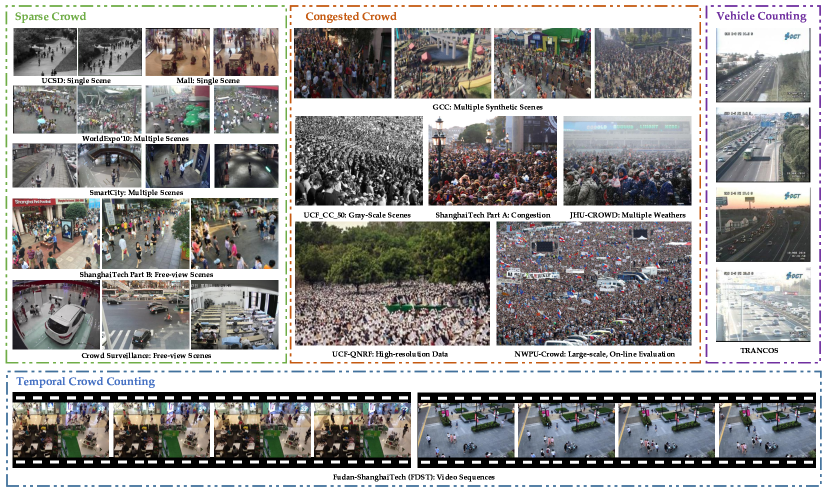
Figure 4: Some samples from representing crowd counting datasets.

III-A Most frequently-used datasets

In this subsection, we introduce some most frequently used crowd counting datasets, i.e., UCSD [27], Mall [40], UCF_CC_50 [38], WorldExpo’10 [51], Shanghai Tech [1], which are listed by chronologically.

$\bullet$ UCSD [27] is the first dataset for crowd counting, which is collected from cameras on the sidewalk. It is composed of 2000 frames with a size of 238$\times$158 and the ground truth annotations of each pedestrian in every five frames. For the rest of frames, the labels are created by using linear interpolation. Since it is collected from a single location, thus there is no change of the perspective view in different frames.

$\bullet$ Mall [40] is a dataset collected from the surveillance video of a shopping mall. The video sequence in the dataset is composed of 2000 frames with a size of 320$\times$240, which contains 62,325 pedestrians in total. Compared with UCSD [27], Mall covers more diversity densities as well as different activity patterns (static and moving persons) under more significant illumination conditions. Additionally, there exists more perspective distortion, resulting in larger size change and appearance of objects, and has severe occlusions due to scene objects.

$\bullet$ UCF_CC_50 [38] is the first really challenging dataset created from publicly available Web images. It includes a variety of densities and different perspective distortions for different scenes such as concerts, protests, stadiums and marathons. Considering that only 50 images in this dataset, a 5-fold cross-validation protocol is conducted on it. Due to the small-scale data volume, even the most advanced recent CNN-based methods are far from optimal for the results on it.

$\bullet$ WorldExpo’10 [51] is a large data-driven cross-scene crowd counting dataset collected from Shanghai 2010 WorldExpo, which includes 1,132 annotated video sequences captured by 108 surveillance cameras. It contains a total of 3920 frames with a size of 576$\times$720, of which 199,923 persons are annotated.

$\bullet$ Shanghai Tech [1] is one of the largest large-scale crowd counting datasets in previous few years which is composed of 1198 images with 330,165 annotations. According to different density distributions, the dataset is divided into two parts: Part_A (SHT_A) and Part_B (SHT_B). SHT_A contains images randomly selected from the Internet, whilst Part_B includes the images are taken from a busy street of a metropolitan area in Shanghai. The density in Part_A is much larger than that in Part_B. This dataset successfully creates a challenging dataset across different scenes types and densities. However, the number of images in different density sets is uneven, which makes the training set and test set tend to be low-density sets. Nevertheless, the scale changes and perspective distortion presented by this dataset provide new challenges and opportunities for the design of many CNN-based networks.

III-B More recently datasets

$\bullet$ Smartcity [9] is created by Tencent YouTu, which contains 50 images in 10 scenes such as sidewalk, office entrance, shopping mall. All of them are high shot for video surveillance. The dataset includes indoor and outdoor scenes, and mainly to verify the generalization ability of the model on very sparse scenes.

$\bullet$ UCF-QNRF [76] is collected from Flickr, Web Search and Hajj footage, which consists of 1,535 challenging images with about 1.25 million annotations. The images in this dataset come with a wider variety of scenes and contain the most diverse set of viewpoints, densities, and lighting variations. However, some of them are so high-resolution that they may lead to memory issues in GPU while training the entire scene.

$\bullet$ City Street [130] is a multi-view video dataset of which the data is collected from a busy city street by using five synchronized cameras, which is composed of 500 multi-view images in total

$\bullet$ ShanghaiTechRGBD [131] is a large-scale RGB-D dataset which consists of 2,193 images with 144,512 labeled head counts. With the crowd scenarios and various lighting condition, making the dataset is the most challenging RGB-D crowd counting dataset regarding the number of head counts.

$\bullet$ FDST [132] is a new large-scale video crowd counting dataset, which consists of 100 videos captured from 13 different scenes including shopping malls, squares, hospitals, etc, which contains 15,000 frames with 394,081 annotated heads, and all with frame-wise annotation.

$\bullet$ Crowd Surveillance [133] contains 13,945 high-resolution images with 386,513 people in total, making the largest and highest average resolution for crowd counting so far. In addition, regions of interest (ROI) annotation is also provided to filter out the regions which are too blurry or ambiguous for training and test.

$\bullet$ JHU-CROWD [134] is a larger dataset w.r.t the number of images and several particular properties such as adverse conditions (weather-based degradations), learning bias mitigated (including distractor images), richer annotations (image-level and head-level in addition to point-level annotations).

$\bullet$ DLR-ACD [135] contains 33 large aerial images with average resolution is 3619$\times$5226, which are captured by standard DSLR cameras installed on an airborne platform on a helicopter. The images come from 16 flight campaigns, and the dataset contains 226,291 person annotations in total.

$\bullet$ DroneCrowd [136] is a drone-based dataset for density map estimation, crowd localization and tracking, simultaneously. The dataset is composed of 112 video sequences with 33,600 frames in total. The average resolution of the frames is 1920$\times$1080, collected from multiple drone devices, 70 different scenarios across four different cities in China. There are more than 4.8 million head annotations on 20,800 people trajectories.

$\bullet$ GCC [84] is collected from an electronic game Grand Theft Auto V (GTA5), named as ”GTA5 Crowd Counting” (GCC for short), which consists of 15,212 images, with resolution of 1080$\times$1920, containing 7,625,843 persons. Compared with the existing datasets, GCC has four advantages: 1) free collection and annotation; 2) larger data volume and higher resolution; 3) more diversified scenes, and 4) more accurate annotations.

$\bullet$ NWPU-Crowd [28] contains 5,109 images with 2,133,238 annotated instances in total. Compared with previous dataset in real world, in addition to data volume, there also some other advantages including negative samples, fair evaluation, higher resolution and large appearance variation.

TABLE III: Statistics of the object counting datasets, including crowd counting and other fields. Total-, min-, average- and max represent the total number, the minimum, average number and maximum number of instances in the datasets, respectively.

Dataset	Year	Attributes	Number of Images	Training/Test	Average Resolution	Count Statistics
						Total	Min	Average	Max
LHI1 [137]	2007	Real-world	–	–	352 $\times$ 288	–	–	–	–
UCSD [27]	2008	Real-world	2000	800/1200	238 $\times$ 158	49,885	11	24.9	46
PETS [138]	2010	Real-world	1076	–	384$\times$288	18289	0	–	40
Mall [40]	2012	Real-world	2000	800/1200	320 $\times$ 240	62,325	13	31	53
UCF_CC_50 [38]	2013	Real-world	50	–	2101 $\times$ 2888	63,974	94	1,280	4,543
AHU-Crowd [139]	2014	Real-world	–	–	–	–	–	–	–
MICC [140]	2014	Real-world	3358	–	–	17630	0	5.25	28
WorldExpo’10 [51]	2015	Real-world	3980	–	576 $\times$ 720	199,923	1	50.2	253
Indoor1 [141]	2016	Real-world	570,000	–	704$\times$576	–	0	–	59
LHI2 [142]	2016	Real-world	3,100	–	1280 $\times$ 720	5,900	–	–	–
AHU-CROWD [143]	2016	Real-world	107	–	–	45,000	58	–	2201
SHT_A [1]	2016	Real-world	482	300/182	589 $\times$ 868	241,677	33	501.4	3,139
SHT_B [1]	2016	Real-world	716	400/316	768 $\times$ 1024	88,488	9	123.6	578
Train Station [144]	2017	Real-world	2000	–	256 $\times$ 256	62581	1	–	53
STF(C5&C9) [144]	2017	Real-world	788$\&$600	–	576 $\times$ 704	–	3	–	65
Shanghai Subway Station [145]	2017	Real-world	3,000	–	–	–	28.78	–	–
Beijing BRT [146]	2018	Real-world	1280	–	640 $\times$ 360	–	1	–	64
EBP [147]	2018	Real-world	–	–	720 $\times$ 408	–	–	–	–
Smartcity [9]	2018	Real-world	50	–	1920 $\times$ 1080	369	1	7.4	14
CrowdFlow [148]	2018	Synthetic	–	–	300$\sim$450	–	–	–	–
UCF-QNRF [76]	2018	Real-world	1,535	1201/334	2013 $\times$ 2902	1,251,642	49	815	12,865
CIISR [149]	2019	Real-world	1000	–	1080 $\times$ 720	–	–	117	–
Venice [86]	2019	Real-world	167	–	1280 $\times$ 720	–	–	–	–
Indoor2 [150]	2019	Real-world	148,243	–	352 $\times$ 288 or 704$\times$576	1,834,770	0	12.4	40
City Street [130]	2019	Real-world	500	300/200	676 $\times$ 380	–	70	–	150
ShanghaiTechRGBD [131]	2019	Real-world	2193	1193/1000	1080 $\times$ 1920	144,512	6	65.9	234
FDST [132]	2019	Real-world	15,000	9000/6000	1920 $\times$ 1080 and 1280 $\times$ 720	394,081	9	26.7	57
Crowd Surveillance [133]	2019	Real-world	13,945	–	1342 $\times$ 840	386,513	–	35	–
JHU-CROWD [134]	2019	Real-world	4250	3888/1062	1450 $\times$ 900	1,114,785	–	262	7286
ZhengzhouAirport [151]	2019	Real-world	1,111	–	–	49,061	7	–	128
DLR-ACD [135]	2019	Aerial imagery	33	19/14	3619 $\times$ 5226	226,291	285	6857	24,368
DroneCrowd [136]	2019	Drone-based	33,600	–	1920 $\times$ 1080	4,864,280	25	144.8	455
Categorized [152]	2019	Categories counting	553	–	–	16,521	1	29.8	206
GCC [84]	2019	Synthetic	15,212	–	1080 $\times$ 1920	7,625,843	0	501	3,995
NWPU-Crowd [28]	2020	Real-world	5,109	–	2311 $\times$ 3383	2,133,238	0	418	20,033
Caltech [153]	2012	Pedestrian detection	2000	–	–	15043	6	–	14
TRANCOS [20]	2015	Vehicle counting	1244	403/420/421	640 $\times$ 480	46,796	9	–	107
Penguins [17]	2016	Penguins counting	80095	–	–	–	0	7.18	67
WIDER FACE [154]	2016	Face detection	32,203	40$\%$/10$\%$/50$\%$	–	393,703	–	–	–
DukerMTMC [155]	2016	tracking, human detection or ReID	over 2 million	–	1920$\times$1080	2,700	–	–	–
WebCamT [156]	2017	WebCam traffic counting	60 million	42,200/17800	352$\times$240	–	–	–	–
CARPK [157]	2017	Drone view-based car counting	1448	989/459	–	89,777	–	–	–
MTC [158]	2017	Planting counting	361	186/175	–	–	–	–
DCC [124]	2018	Cell counting	177	100/77	–	–	0	34.1	101
Wheat-Spike [159]	2018	wheat spikes counting	20	8/2/10	1k$\sim$3k	20,101	749	1005	1287
VisDrone2019 People [160]	2018	Drone-based crowd counting	3347	2392/329/626	969$\times$1482	108,464	10	32.41	289
VisDrone2019 Veheicle [160]	2018	Drone-based vehicle counting	5303	3953/364/986	991$\times$1511	198,984	10	37.52	349

III-C Some special crowd counting datasets

In this subsection, we briefly introduce some special crowd counting datasets, which are only used in some certain scenarios. These datasets contain line crowd counting (LHI [137, 142], crowd sequences (PETS [138], Venice [86]), multi-sources (AHU-Crowd [139, 143], CIISR [149], Venice [86]), indoor (MICC [140], Indoor¹ [141], Indoor² [150]), train station (TS [144], STF [144]), subway station (Shanghai Subway Station [145]), BRT (Beijing BRT [146]), bridge (EBP [147]), airport (ZhengzhouAirport [151]), categorized [152]. The specific statistics of these datasets are listed in Tabel III.

III-D Representing object Counting datasets in other fields

For completeness, we introduce some representing object counting dataset in other fields, to verify the generalization ability of the designed model further.

$\bullet$ Caltech [153] is a dataset for pedestrian detection, which has 2000 images and 15043 pedestrians in total. The dataset can be used to verify the performance of the algorithms in sparse scenes.

$\bullet$ TRANCOS [20] is the first one for vehicle counting in traffic jam images. The dataset is often used to evaluate the generalization ability of the crowd counting methods.

$\bullet$ The penguin dataset [17] is a product of an ongoing project for monitoring the penguin population in Antarctica.The dataset can be used to study climate change, etc.

$\bullet$ WIDER FACE [154] is a large-scale face detection benchmark, which is composed of 32,203 images in total and 393,703 faces with bounding boxes annotations.

$\bullet$ DukerMTMC [155] is a multi-view video dataset for multi-view tracking, human detection and re-identification (ReID), which contains over 2 million frames and more than 2,700 identities.

$\bullet$ WebCamT [156] is the first largest annotated webcam traffic dataset to date, which consists of 60 million frames collected from 212 web cameras with different locations, camera perspective, and traffic states.

$\bullet$ CARPK [157] is a car counting datasets collected from 4 different parking lots with drone view, which contains nearly 90,000 cars in total, all the images with bounding box annotations.

$\bullet$ MTC [158] includes 361 high-resolution images of maize tassels in the wild filed. Compared with the other objects that have similar physical sizes, maize tassels have the heterogeneous physical sizes and self-changing over time. Thus it is more suitable for evaluating the robustness to object-size variations of the designed model.

$\bullet$ DCC [124] is a cell microscopy dataset, which contains 177 images with a variety of tissues and species. Across these images, the average count is 34.1, and the standard deviation is 21.8.

$\bullet$ Wheat-Spike [159] is a challenging dataset due to irregular placement or collection of wheat spikes, which contains 20 images in total, where the data are split into 8, 2 and 10 for training, validation and test.

$\bullet$ VisDrone2019 [160] originates from an object detection dataset with bounding boxes annotated, Bai et al. [161] takes the center of bounding box as the location of objects, selecting pedestrian and people to form VisDrone2019 People dataset, and combining car, van, truck and bus to construct VisDrone2019 Vehicle dataset.

IV Evaluation metrics

There are several ways to evaluate the performance between predicted estimations and ground truths. In this section, we review some universally-agreed and popularly adopted measures for crowd counting model evaluation. According to different evaluation criteria, we divide the evaluation metrics into three categories: image-level for evaluating the counting performance, pixel-level for measuring the density map quality and point-level for assessing the precision of localization.

IV-A Image-level metrics

Two most common used metrics are Mean Absolute Error (MAE) and Mean Square Error (RMSE), which are defined as follows:

$$\footnotesize MAE=\frac{1}{N}\sum_{i=1}^{N}\left|C_{I_{i}}^{pred}-C_{I_{i}}^{gt}\right|,$$ (1)

$$\footnotesize RMSE=\sqrt{\frac{1}{N}\sum_{i=1}^{N}\left|C_{I_{i}}^{pred}-C_{I_{i}}^{gt}\right|^{2}},$$ (2)

where $N$ is the number of the test image, $C_{I_{i}}^{\text{ pred }}$ and $C_{i}^{gt}$ represent the prediction results and ground truth, respectively. Roughly speaking, $MAE$ determines the accuracy of the estimates, while $RMSE$ indicates the robustness of the estimates.

Considering aforementioned $MAE$ may loss the location information, to provide a more accurate evaluation, Guerrero et al. [20] propose a new metric is Grid Average Mean Absolute Error (GAME), which is defined as follows:

$$\footnotesize GAME(L)=\frac{1}{N}\sum_{n=1}^{N}\left(\sum_{l=1}^{4^{L}}\left|C_{I_{i}}^{pred}-C_{I_{i}}^{gt}\right|\right),$$ (3)

where $4^{L}$ denotes that dividing the image into some non-overlapping regions. The higher $L$, the more restrictive of the GAME metric will be. Note that when $L=0$, $GAME$ will degenerate into $MAE$.

Similarly, accounting for the localization errors, a mean pixel-level absolute error (MPAE) [162] is proposed as follows:

$$\footnotesize\mathrm{MPAE}=\frac{\sum_{i=1}^{N}\sum_{j=1}^{H}\sum_{k=1}^{W}\left|D_{i,j,k}-\hat{D}_{i,j,k}\right|\times 1_{\left\{D_{i,j,k}\in R_{i}\right\}}}{N},$$ (4)

where $D_{i,j,k}$ denotes the ground-truth density map of $i$-th image at the pixel ($j$,$k$), $\hat{D}_{i,j,k}$ means the corresponding estimated density map, $R_{i}$ represents the ROI of the $i$-th image, $1_{\{\cdot\}}$ indicates the indicator function, and $W$, $H$ and $N$ are the width, height and the number of test samples. MPAE measures the degree of wrongly localized the densities are.

In view of both $MAE$ and $RMSE$ are the metrics for global accuracy and robustness, which cannot evaluate the local regions, thus Tian et al. [79] expand $MAE$ and $RMSE$ to patch mean absolute error ($PMAE$) and patch mean squared error ($PMSE$), which are defined as

$$\footnotesize PMAE=\frac{1}{m\times N}\sum_{i=1}^{m\times N}\left|C_{I_{i}}^{pred}-C_{I_{i}}^{gt}\right|,$$ (5)

$$\footnotesize PMSE=\sqrt{\frac{1}{m\times N}\sum_{i=1}^{m\times N}\left(C_{I_{i}}^{pred}-C_{I_{i}}^{gt}\right)^{2}},$$ (6)

where $m$ is the splitted non-overlapping patches. Note that when $m$ equals to 1, $PMAE$ and $PMSE$ degenerate into $MAE$ and $RMSE$, respectively.

IV-B Pixel-level metrics

Two metrics named Peak Signal to Noise Ratio (PSNR) and Structural Similarity Index (SSIM) [125] are usually used to measure the quality of the generated density map. Specifically, PSNR, the most common and widely used evaluation index of the image, which is essentially based on the error between corresponding pixels, in other words, error sensitivity. Generally speaking, high values represent smaller errors. However, it does not take the human visual characteristics into account, for example, the human is more sensitive to the contrast difference of lower spatial frequency and more sensitive to the brightness than hue, the perceptual results of a region is influenced by surrounding adjacent regions, etc. Therefore, the evaluation results are often inconsistent with people’s subjective feelings.

In addition, SSIM [125] measures the image similarity from three aspects: brightness, contrast and structure, which can be regarded as the multiplication of the three parts. The value of SSIM is in the range of [0,1], the larger of the value, the less distortion of the image.

IV-C point-level metrics

To evaluate the localization performance of the model, Average Precision (AP) and Average Recall (AR) are two most common used metrics. Generally speaking, when the value of AP increases, AR decreases. Thus how to trade off between them is a worthy considering question.

V Benchmarking and analysis

V-A Overall benchmarking results evaluation

Table IV presents results of 53 state-of-the-art CNN-based methods and 7 representative traditional approaches over six mainstream benchmark datasets in crowd counting task. Two widely used evaluation metrics, i.e., MAE and RMSE are for measuring the accuracy and robustness of the models. All the models are representative and the results listed in the Table IV are published in their papers or reported by other works .

$\bullet$ CNN-based v.s. traditional models. Comparing the traditional models with CNN-based ones in Table IV, as excepted, we observe that CNN-based methods make great improvement of performances by a large margin. It also demonstrates that strong feature learning ability of deep convolution neural network based on large-scale annotated data.

$\bullet$ Performance comparison of CNN-based models. Since the year of 2015, the first CNN-based density map estimation model was proposed for crowd counting, the performance has also been improved gradually over time, which has witnessed the significant progress of the crowd counting model. Among the deep models, Cross scene [51] performs the worst performance, as the first ones to apply CNNs for crowd counting, which adopts the basic network structure and handle the cross-scene problem that transfers the pre-trained CNN to unseen scenes. Thus the model is lower compared with the single-scene and domain-specific model. However, this work provides a good solution to the generalizing trained model to unseen scenes.

V-B Properties-based evaluation

We choose three top-performing models in terms of MAE and RMSE over six commonly used datasets, ending up with collecting 19 models, including two heuristic models, i.e., MCNN [1] and CSRNet [12], the main properties of these state-of-the-arts are listed in Table V. These properties cover the main techniques that could be used to explain the reason they perform well.

From Table V, we can find that, among these state-of-the-art methods, two-thirds of which adopt single column network architecture. For this phenomenon, perhaps we can reach the following conclusion: instead of making the network wider, deeper networks may be better. In addition, more than one third of them incorporate visual attention mechanism [71, 7, 83, 8, 13, 89, 87, 97] and dilation convolution layer [12, 80, 81, 83, 84, 86, 163] into their frameworks. Instead of using all available information of the input image in many CNNs-based methods, the visual attention mechanism is to use pertinent information to compute the neural responses, which can learn to weight the importance of each pixel of feature maps. Due to the prominent ability, visual attention mechanism has been applied to many computer vision tasks, such as image classification [164], semantic segmentation [165], image deblurring [166], and visual pose estimation [167], it is also suitable for the problem of crowd counting, highlighting the regions of interest containing the crowd and filtering out the noise in the background clutter situations. Dilated convolution layers, a good alternate of the pooling layer, have demonstrated that significant improvement of accuracy in segmentation tasks [168, 169, 170]. The advantage of the dilation convolution layer is that enlarging receptive field without information loss caused by pooling operations (max and average pooling, etc.) and without increasing the number of parameters and the number of computations (such as up-sampling operations of the de-convolution layer in FCN [171]). Therefore, the dilation convolution layer can be integrated into the crowd counting framework to capture more multi-scale features and maintain more detailed information.

Spatial Transformer Network (STN) [105] and deformable convolution [172] have a similar effect to address the problem of rotation, scaling or warping, which limit the capacity of feature invariance of standard CNNs. Specifically, STN is a sub-differential sampling module, which requires no extra annotations and has the capacity of adaptively learning spatial transformation between different data. It can not only carry out the spatial transformation on the input image but also any layer of the convolutional layer to realize the spatial transformation of different feature maps. Due to the remarkable performance, STN has been applied to many communities, such as multi-label image recognition [173] and saliency detection [174]. Therefore, it also adopted by Liu et al. [71] to address the scale and rotation variation in crowd counting.

Conditional random fields (CRFs) [175] or Markov Random Fields (MRFs) [176] have been usually leveraged as a post-possessing operation to refine the features and outputs of the CNNs with a message passing mechanism [177]. In the work of  [178], the first to utilize CRFs to refine features with different scales for the crowd counting task and demonstrates the effectiveness on the benchmark datasets. Zhang et al. [179] propose an attentional neural fields (ANF) framework which integrates CRFs and non-local operation [180] (similar as self-attention) for crowd counting.

Perspective distortion is a major challenge in the crowd counting, while perspective information may be provided in two ways: one is related to camera’s 6 degree-of-freedom (DOF) [181], the other is to identify the scale variation in the distance from the camera in the counting task. It can provide additional information with respect to scale variation and perspective geometry, many traditional crowd counting methods [27, 182] utilize it to normalize the regression features or detection features of changeable scales. Some modern CNNs-based methods also use perspective information to infer the ground truth density [51, 1] or body part maps [183]. These methods utilize perspective information yet without using the perspective map. Instead, some works [86, 85] leverage it to encode global or local scales in the network.

Spatial pyramid pooling (SPP) [184] was originally raised for visual recognition, which has several advantages than traditional networks, firstly it adapts the input images with arbitrary sizes; additionally, as the pooling layers with different sizes are extracted from the feature map and then aggregating them into a vector with fixed length, so that improve the robustness and accuracy. Moreover, it can accelerate convergence speed. Therefore, it is used to capture and fuse multi-scale features in SCNet [185], PaDNet [79] and CAN [86] for crowd counting.

Pan-density crowd counting aims to deal with two phenomena in crowd scenarios: varying densities and distributions in different scenarios and inconsistent densities of local regions in the same scene. Most current methods are designed for a specific density or scenario so that it is difficult to take full advantage of pan-density information. Although many multi-column architectures are designed to cope with this problem, such as MCNN [1], Switch-CNN [5] and CP-CNN [6], they always suffer from low efficiency, high computation complexity, and biased local estimation. However, PaDNet [79] is put forward to provide a reasonable solution to effectively identify specific crowd by the sub-networks in Density-Aware Network (DAN), and learn an enhancement rate for each feature map by a Feature Enhancement Layer (FEL). In the final, these feature maps are fused to obtain better counting.

TABLE IV: Comparison of the performance of different methods on the representing crowd counting datasets. Red, green and blue indicate the first, the second and the third best performance, respectively. Note that the MAE in WorldExpo’10 [51] is the average value of the five cross-scenes, SFCN${\dagger}^{2}$ [84] represents that model takes ResNet101 as backbone, pre-trained on GCC [84], ”–” denotes that results are not available and ”$\downarrow$” indicates the lower the better of the results.

#	Methods	Year$\&$Venue	UCSD [27]		Mall [40]		UCF_CC_50 [38]		WorldExpo’10 [51]		SHT_A [1]		SHT_B [1]		UCF-QNRF [76]
			MAE$\downarrow$	RMSE$\downarrow$	MAE$\downarrow$	RMSE$\downarrow$	MAE$\downarrow$	RMSE$\downarrow$	MAE$\downarrow$	RMSE$\downarrow$	MAE$\downarrow$	RMSE$\downarrow$	MAE$\downarrow$	RMSE$\downarrow$	MAE$\downarrow$	RMSE$\downarrow$
1	GP [27]	2008 CVPR	2.24	7.97	3.72	20.1	–	–	–	–	–	–	–	–	–	–
2	Lempitsky et.al [16]	2010 NIPS	1.70	–	–	–	493.4	487.1	–	–	–	–	–	–	–	–
3	LBP+RR [40]	2012 BMVC	–	–	–	–	–	–	31.0	–	303.2	371.0	59.1	81.7	–	–
4	Idrees 2013 [38]	2012 CVPR	–	–	–	–	468.0	590.3	–	–	–	–	–	–	315.0	508.0
5	CA-RR [54]	2013 CVPR	2.07	6.86	3.43	17.7	–	–	–	–	–	–	–	–	–	–
6	Faster RCNN [34]	2015 NIPS	–	–	5.91	6.60	–	–	–	–	–	–	44.51	53.22	–	–
7	Count-Forest [48]	2015 ICCV	1.61	4.40	2.50	10.0	–	–	–	–	–	–	–	–	–	–
8	Cross-scene [51]	2015 CVPR	1.60	3.31	–	–	467.0	498.5	12.9	–	181.8	277.7	32.0	49.8	–	–
9	MCNN [1]	2016 CVPR	1.07	1.35	2.24	8.5	377.6	509.1	11.6	–	110.2	173.2	26.4	41.3	–	–
10	MSCNN [186]	2017 ICIP	–	–	–	–	363.7	468.4	11.7	–	83.8	127.4	17.7	30.2	–	–
11	CMTL [55]	2017 AVSS	–	–	–	–	322.8	397.9	–	–	101.3	152.4	20.0	31.1	252	514
12	Switching CNN [5]	2017 CVPR	1.62	2.10	–	–	318.1	439.2	9.4	–	90.4	135.0	21.6	33.4	228	445
13	CP-CNN [6]	2017 ICCV	–	–	–	–	295.8	320.9	8.86	–	73.6	106.4	20.1	30.1	–	–
14	SaCNN [9]	2018 WACV	–	–	–	–	314.9	424.8	8.5	–	86.8	139.2	16.2	25.8	–	–
15	ACSCP [74]	2018 CVPR	1.04	1.35	–	–	291.0	404.6	7.5	–	75.7	102.7	17.2	27.4	–	–
16	CSRNet [12]	2018 CVPR	1.16	1.47	–	–	266.1	397.5	8.6	–	68.2	115.0	10.6	16.0	120.3	208.5
17	IG-CNN [72]	2018 CVPR	–	–	–	–	291.4	349.4	11.3	–	72.5	118.2	13.6	21.1	–	–
18	DecideNet [7]	2018 CVPR	–	–	1.52	1.90	–	–	9.23	–	–	–	21.53	31.98	–	–
19	DRSAN [71]	2018 IJCAI	–	–	1.72	2.1	219.2	250.2	7.76	–	69.3	96.4	11.1	18.2	–	–
20	ic-CNN (two stages) [73]	2018 ECCV	–	–	–	–	260.9	365.5	10.3	–	68.5	116.2	10.7	16.0	–	–
21	SANet [11]	2018 ECCV	1.02	1.29	–	–	258.4	334.9	8.2	–	67.0	104.5	8.4	13.6	–	–
22	SCNet [185]	2018 arXiv	–	–	–	–	280.5	332.8	6.4	–	71.9	107.9	9.3	14.4	–	–
23	MA-Net [187]	2019 TCSVT	–	–	1.76	2.2	245.4	349.3	8.34	–	61.8	100.0	8.6	13.3	–	–
24	PaDNet [79]	2019 TIP	0.85	1.06	–	–	185.8	278.3	–	–	59.2	98.1	8.1	12.2	96.5	170.2
25	ASD [80]	2019 ICASSP	–	–	–	–	196.2	270.9	–	–	65.6	98.0	8.5	13.7	–	–
26	SAA-Net [13]	2019 CVPR	–	–	–	–	238.2	310.8	–	–	63.7	104.1	8.2	12.7	97.5	167.8
27	PACNN [85]	2019 CVPR	0.89	1.18	–	–	267.9	357.8	7.8	–	66.3	106.4	8.9	13.5	–	–
28	SFCN${\dagger}^{2}$ [84]	2019 CVPR	–	–	–	–	214.2	318.2	–	–	64.8	107.5	7.6	13.0	102.0	171.4
29	CAN(ECAN) [86]	2019 CVPR	–	–	–	–	212.2	243.7	7.4 (7.2)	–	62.3	100.0	7.8	12.2	107	183
30	SFANet [89]	2019 arXiv	0.82	1.07	–	–	219.6	316.2	–	–	59.8	99.3	6.9	10.9	100.8	174.5
31	CFF [87]	2019 ICCV	–	–	–	–	–	–	–	–	65.2	109.4	7.2	12.2	–	–
32	DUBNet [188]	2019 AAAI	1.03	1.24	–	–	235.2	332.7	–	–	66.4	111.1	9.4	15.1	116	178
33	CTN [189]	2019 arXiv	–	–	–	–	219.3	331.0	–	–	64.3	107.0	8.6	14.6	–	–
34	DENet [190]	2019 arXiv	1.05	1.31	–	–	241.9	345.4	8.2	–	65.5	101.2	9.6	15.4	–	–
35	W-Net [90]	2019 arXiv	0.82	1.05	–	–	201.9	309.2	–	–	59.5	97.3	6.9	10.3	–	–
36	DSNet [163]	2019 arXiv	0.82	1.06	–	–	183.3	240.6	–	–	61.7	102.6	6.7	10.5	91.4	160.4
37	SAAN [8]	2019 WACV	–	–	1.28	1.68	271.6	391.0	–	–	–	–	16.86	28.41	–	–
38	ADCrowdNet [83]	2019 CVPR	1.09	1.35	–	–	273.6	362.0	7.3	–	70.9	115.2	7.7	12.9	–	–
39	PSDDN [56]	2019 CVPR	–	–	–	–	359.4	514.8	–	–	85.4	159.2	16.1	27.9	–	–
40	TEDnet [92]	2019 CVPR	–	–	–	–	249.4	354.5	8.0	–	64.2	109.1	8.2	12.8	113	188
41	SPN [81]	2019 WACV	1.03	1.32	–	–	259.2	335.9	–	–	61.7	99.5	9.4	14.4	–	–
42	PCC Net [88]	2019 TCSVT	–	–	–	–	240.0	315.5	9.5	–	73.5	124.0	11.0	19.0	132	191
43	RAZ-Net [94]	2019 CVPR	–	–	–	–	–	–	8.0	–	65.1	106.7	8.4	14.1	116	195
44	RReg(MCNN) [93]	2019 CVPR	–	–	–	–	–	–	8.7	–	72.6	114.3	15.5	23.1	–	–
45	RReg(CSRNet) [93]	2019 CVPR	–	–	–	–	–	–	8.5	–	63.1	96.2	8.72	13.56	–	–
46	AT-CFCN [95]	2019 CVPR	–	–	2.28	2.90	–	–	–	–	–	–	11.05	19.66	–	–
47	AT-CSRNet [95]	2019 CVPR	–	–	–	–	–	–	7.8	–	–	–	8.11	13.53	–	–
48	IA-DCCN [191]	2019 CVPR	–	–	–	–	264.2	394.4	–	–	66.9	108.4	10.2	16.0	125.3	185.7
49	HA-CCN [97]	2019 TIP	–	–	–	–	256.2	348.4	–	–	62.9	94.9	8.1	13.4	118.1	180.4
50	L2SM [98]	2019 ICCV	–	–	–	–	188.4	315.3	–	–	64.2	98.4	7.2	11.1	104.7	173.6
51	DSSINet [178]	2019 ICCV	–	–	–	–	216.9	302.4	6.67	–	60.63	96.04	6.85	10.34	99.1	159.2
52	BL [192]	2019 ICCV	–	–	–	–	229.3	308.2	–	–	62.8	101.8	7.7	12.7	88.7	154.8
53	LSC-CNN [57]	2019 ICCV	–	–	–	–	225.6	302.7	8.0	–	66.4	117.0	8.1	12.7	120.5	218.2
54	SANet [11]+SPANet [193]	2019 ICCV	1.00	1.28	–	–	232.6	311.7	7.7	–	59.4	92.5	6.5	9.9	–	–
55	MBTTBF-SCFB [194]	2019 ICCV	–	–	–	–	233.1	300.9	–	–	60.2	94.1	8.0	15.5	97.5	165.2
56	S-DCNet [195]	2019 ICCV	–	–	–	–	204.2	301.3	–	–	58.3	95.0	6.7	10.7	104.4	176.1
57	PGCNet [133]	2019 ICCV	–	–	–	–	259.4	317.6	8.1	–	57.0	86.0	8.8	13.7	–	–
58	ANF [179]	2019 ICCV	–	–	–	–	250.2	340.0	8.1	–	63.9	99.4	8.3	13.2	110	174
59	RANet [99]	2019 ICCV	–	–	–	–	239.8	319.4	–	–	59.4	102.0	7.9	12.9	111	190
60	ACSPNet [196]	2019 Neurocomputing	1.02	1.28	1.76	2.24	275.2	383.7	9.8	–	85.2	137.1	15.4	23.1	–	–

TABLE V: Main properties of state-of-the-art methods.

	Multi-column	Single-column	Attention-based	Dilation convolution	Spatial transformer	CRFs/MRF	Perspective information	Pyramid pooling	Pan-density /sub-region
MCNN [1]	✓						✓		✓
CSRNet [12]		✓		✓
DRSAN [71]	✓		✓		✓
DecideNet [7]	✓		✓
SCNet [185]		✓		✓				✓
PaDNet [79]	✓							✓	✓
SAAN [8]	✓		✓
PACNN [85]		✓					✓
CAN&ECAN [86]		✓		✓			✓	✓
SFANet [89]		✓	✓
W-Net [90]		✓	✓
DSNet [163]		✓		✓
L2SM [98]		✓
DSSINet [178]	✓		✓	✓		✓
SPANet [193]	✓								✓
MBTTBF-SCFB [194]	✓		✓			✓
BL [192]		✓
S-DCNet [195]		✓							✓
PGCNet [133]		✓					✓

Comprehensively considering the statistical results from Table V and the analysis of various methods, we make the following observations:

$\bullet$ Among the CNN methods, most networks are based on single column network architecture, which is more simpler yet effective than multi-column architectures that are high complexity and bloated structure as demonstrated in  [12].

$\bullet$ The techniques of visual attention mechanism, dilation convolution, and spatial pyramid pooling (SPP) can significantly improve the performance of the final estimation and the quality of density maps.

$\bullet$ Incorporating perspective information [51, 1, 86, 85] into the network can provide additional support and guidance for the extraction of multi-scale features.

$\bullet$ Spatial transformer network [105, 71] and deformable convolution [172, 83] can help to address the rotation and uniform distributions of crowds which is more suitable for the crowd understanding problem in the congested noisy scenarios.

$\bullet$ Pan-density learning [79] can not only take full advantages of global features but also make up biased local estimation.

$\bullet$ Multi-pathway or multi-task framework [7, 80, 89] followed by jointly loss function can improve the estimation performance and speed up the training.

V-C Attributes-based analysis

Albeit significant performance improvement has been achieved to a great extent by applying CNNs into density map estimation crowd counting models, there are remain some challenges to be conquered. A robust network should have the capability of coping with various complex scenarios. The existence of challenges always brings many difficulties to the models, such as occlusion, scale variation, perspective distortion, rotation, illumination variation, and weather changes. Some samples are shown in Fig. 5. Moreover, the scenes of the images are from indoor, outdoor, and in the wild. It is worth noting that these attributes are not mutually exclusive. In other words, there may exist several attributes in one image. We also take the aforementioned methods in Table V as an example to analyze these attributes in detail.

Figure 5: The challenges in crowd counting.

$\bullet$ Occlusion. As the crowd density increasing, the crowd will appear to occlude each other partly, which limits the capacity ability of traditional detection algorithms and prompts the emergence of density estimation models.

$\bullet$ Complex background. Background regions (have no person instances) includes confusing objects or have similar appearance or colors with the foreground, this can be suppressed through semantic segmentation or visual attention operations, such as [71, 7, 83, 8, 13, 89, 197].

$\bullet$ Scale variation. The most primary problem should be addressed in the density estimation models, as the scales of objects (such as the sizes of people heads) vary as the distance from the camera. Therefore, almost all the density estimation models are designed for addressing the scale variation problem in the first step.

$\bullet$ Non-uniform distribution. For intuitive understanding in the examples of Fig. 5, we can observe that diverse densities and distributions in different scenes and inconsistent distributions of local regions even in the same scene. The problem can be effectively addressed in the work of  [198], which presents the first model to estimate various crowd densities with different regressors. Jiang et al. [151] tackle this issue by proposing a multi-level convolution neural network (MLCNN) which fuses multiple density maps generated by multi-level features. This problem can also be regarded as pan-density crowd counting, and related solutions can be referred to PaDNet [79].

$\bullet$ Perspective distortion. Perspective distortion would drastically lead to person scale variation in the crowding counting scenes, which is related to camera calibration to estimate the 6 degree-of-freedom (DOF) of a camera.

$\bullet$ Rotation. The issue of rotation variation drastically due to the camera viewpoints such as different pose and photographic angles, it is addressed by the work  [71] via incorporating spatial transformer network (STN) into LSTM framework.

$\bullet$ Illumination variation. The illumination varies at different times in a day, usually from dark to light and then to dark, from dawn to dusk.

$\bullet$ Weather changes. The scenes in the wild usually under various types of weather conditions, such as clear, clouds, rain, foggy, thunder, overcast, and extra sunny.

The above challenges promote us to design more effective and robust frameworks to address these issues, and this also indicates that there is still much research room in the direction of crowd counting.

VI Discussion

In this section, we discuss some important factors that will directly affect the performance of the crowd counting model design and some promising research directions.

VI-A Model design

$\bullet$ Ground truth density maps generation. As a cornerstone towards CNN-based density estimation and crowd counting models, the generation of high-fidelity ground truth density maps is essential to data preparation for training. To convert an image with the original labels (generally refer to head location) to a density map, Lempitsky et al. [16] first raised and defined as a sum of Gaussian kernels centered on the locations of objects. This strategy works well for characterizing the density distribution of circle-like objects such as cells and bacteria. To tackle scale variations, Zhang et al. [51] put forward a solution by exploiting perspective information: the density map can be obtained by a sum of Gaussian kernels as a head part and a bivariate normal distribution. However, this strategy introduces a new issue of acquiring the perspective map. Fortunately, Zhang et al. [1] find that head size is related to the distance between two neighboring persons. Based on it, a geometry-adaptive kernel-based density map generation method is created, which inspires lots of works adopting this tool to prepare their data training. Although such strategy works well in the dense crowd scenes, it would fail in the sparse scenes. A depth-adaptive kernel-based density map generation method [131] is proposed by positing that the sizes of all heads are the same in the real world.

However, all the methods above are not content-aware. Therefore, Oghaz et al. [199] propose a brute-force nearest neighbor search technique to provide the absolute nearest neighbors despite the distribution of points, through using an integration of Chan-Vese segmentation algorithm, two-dimension Gaussian filter and brute-force nearest neighbor search technique. Recently, Xu et al. [115] claim that the target density map generation manner may fail in the dense regions, since the density map is given by the sum of severely overlapped Gaussian blobs, which leads to diverse density patterns different from the sparse regions. Therefore, a learning-to-scale module (L2SM) is applied to re-scale the dense regions into similar scale levels, so as to ameliorate the pattern shifts and increase the counting accuracy. In another way, Ma et al. [192] propose a Bayesian loss to enforce a more reliable density contribution probability model from the point-annotations. Olmschenk et al. [200] propose an inverse k-nearest neighbor (ikNN) map to supersede the density maps, which can offer a smooth training gradient and accurate localization simultaneously, this also breaks the routine and opens new paths for us. Wan et al. [201] propose an adaptive density map generator that generates a learnable density map representation from the ground truth dot labels.

Anyway, the proper selecting for density map generation will lay a solid foundation for the crowd counting.

$\bullet$ Loss function. The customized design of loss function is also an essential procedure in training effective models. Density map estimation CNN-based crowd counting methods are mostly a regression task, which usually adopt Euclidean distance as loss function to measure the difference between the estimated density map and ground truth. Although widely used, only the Euclidean loss employed may have some disadvantages such as sensitivity to outliers and image blur, pixel independent assumption neglecting the local coherence, and spatial correlation in density maps. Therefore, SmoothL1 loss [33] and Tukey Loss [202] are more robust for outliers can be leveraged, as described in  [113]. Besides, an adversarial loss [103] is integrated to address the issue and improve the quality of density maps [6, 74, 203]. Nevertheless, density maps may contain little high-level semantic information, thus a light-weight SSIM local pattern consistency loss combined with Euclidean loss to enforce the local structural similarity between estimated density maps and ground truths [11], but it only can tackle the local consistent of regions with a fixed size. Therefore, further, a Dilated Multi-scale Structure Similarity (DMS-SSIM) loss [178, 204] is utilized to make the network learn the local similarity within the regions of varied sizes and generate the density maps with local consistency. Besides, a novel scale-aware loss function to specialize person head on a particular scale [13]. Additionally, a combination of spatial abstraction loss (SAL) and the spatial correlation loss (SCL) are provided in [92] to improve density map quality. In another way, accounting for the spatial variation of density, a Maximum Excess over Pixels (MEP) loss [193] is proposed to optimize the pixel-level subregion which has a high discrepancy with the ground-truth density map.

Overall, designing appropriate loss functions helps boost the performance of the models.

$\bullet$ Information fusion of multi cues. Generally, the information fusion of multiple cues can significantly improve the performance of the algorithm, for instance, the integration of scale-aware and context-aware would boost the performance [86, 6], the combination of different pathways for sparse and dense scenarios [7, 80, 89]. Meanwhile, heterogeneous attributes, such as geometric/semantic/numeric attributes are leveraged to assist the density estimation for crowd counting [95].

As a whole, there is an abundant of data availability across many different data sources or modalities in various formats. Fusing these heterogeneous cues with ”broad learning” may be a reliable research direction.

$\bullet$ Network Topology. The network topology represents the information flow within the network, which influences the training complexity and parameters that are required. Proved by many experiments, the encoder-decoder pipeline appears promising performance for the crowd counting task, for instance, CSRNet [12] adopts a standard encoder-decoder structure, which takes a pre-trained VGG16 [205] as a backbone, and builds dilated convolution operation in the decoder. SA-Net [11] presents a similar model, which uses Inception model [109] in the encoder and Transposed convolution layers in the decoder. W-Net [90] directly leverages U-Net [110] structure with VGG16 [205] replacing the encoder block, and adds a extra branch for faster convergence. TEDnet [92] deploys an encoder-decoder hierarchy in a trellis manner. SGANet [206] investigates the effectiveness of Inception-v3 [207] for crowd counting. Beyond encoder-decoder pipeline, VGG16 [205] is the best backbone for feature extraction among VGG16bn, Resnet50 [208] and Inception [109], which has been empirically demonstrated in [90] and strong transfer ability for crowd analysis.

VI-B Dataset construction

In light of previous observation, we would put forward some suggestions for the construction of crowd counting dataset, w.r.t., scene diversity, multi-view, annotation accuracy, etc.

$\bullet$ Scene diversity. Some earlier datasets for crowd counting is in single-scene, i.e., the images are from the same video sequence, which has no variation in the perspective across different images, such as UCSD [27] and Mall [40], as illustrated in Fig. 4.

To meet the need of cross-scene and diversified data for deep model training, some more challenging datasets are proposed, including UCF_CC_50 [38], SHT_A [1], UCF_QNRF [76], and countless others. Nevertheless, there are some drawbacks that limit their generation ability, for instance, UCF_CC_50 [38] is limited by the small number of availability of high-resolution crowd images, SHT_A [1] is suffered from non-uniform density level and inaccurate labels of some samples. UCF_QNRF [76] has the most number of high-count crowd images and annotations with diverse densities, which is more significant than UCF_CC_50 [38], however, the intra-class variation may sometimes exceed the capability of the network. Notably, they may tackle some unseen extreme cases when transferring the data to the wild, such as weather change and illumination variation. GCC [84] may provide a reasonable solution by constructing a large-scale synthetic crowd counting, which consists of more diverse scenes to mimic the challenges in the wild better. Albeit plenty of data in GCC [84], there exists a large “domain gap” between synthetic and real data.

$\bullet$ Multi-view. Previous datasets are for single-view counting, which cannot satisfy the requirements of large and wide scenes, taking public parks or long queue in train station as an example, the scene is so wide that cannot be fully captured by single view, so long that too low of the resolution away from the camera, or most of the crowds are occluded by large objects. Some attempts have been made to tackle the shortcoming, for example, City street dataset [130] is collected from a busy street intersection, which contains large range crowds with more complex occlusion patterns and large scale variations.

$\bullet$ Annotation accuracy. There exists an intrinsic shortcoming in the existing dense crowd counting dataset, the annotations are not very accurate, such as some samples are from UCF_CC_50 [38] and Shanghai Tech Part_A [1]. In fact, this problem is inevitable due to data annotated by different subjects or following different standards.

$\bullet$ Annotation tools. Effective annotation tools are critical in the process of dataset construction. We strongly recommend an online efficient annotation tool based on HTML5 + Javascript + Python, which supports two types of label form, i.e., point and bounding box. During the process of annotation, images are adaptively zoomed in/out to annotate heads according to different scales, and each of them are divided into $16\times 16$ blocks, which provides five scales for the annotators, specifically $2^{(}i)$ ($i=0,1,2,3,4$) times size of the original image. This annotation tool can effectively improve the annotation speed and quality. With the aid of this effective annotation tool, we construct a large-scale dataset named as NWPU-Crowd [28], and more detailed description is shown in the video demo at https://www.youtube.com/watch?v=U4Vc6bOPxm0/. Moreover, some mainstream models are benchmarked on our NWPU-Crowd [28] dataset, the code of which are open-sourced at https://github.com/gjy3035/NWPU-Crowd-Sample-Code. and more detailed results are at https://www.crowdbenchmark.com/nwpucrowd.html.

As a whole, constructing cross-scene, multi-view and accurately annotated datasets which able to more faithfully reflect the real world challenge is essential to boost the generalization ability of crowd counting. Additionally, effective annotation tools are vital for the construction of the datasets.

VI-C The quality of density maps

Most existing methods pay attention to the count rather than the quality of density maps, which is an essential factor that affects the performance. Sindagi [6] first observed this issue and proposed to incorporate global context into the training process while used adversarial loss together with Euclidean loss to obtain shaper and high-quality density maps. We choose several representing methods that concentrate the quality of density maps in terms of two measures, i.e., PSNR and SSIM [125], as illustrated in Table VI. From the table, we can see that SE Cycle GAN [84] shows the worst performance. We suspect it should be attributed to the “domain gap” between synthetic data and real-world data.

TABLE VI: Comparison of the quality of density maps on the SHT_A dataset [1] in terms of PNSR and SSIM [125]. Red and underline indicate the best and the worst performance, respectively. ”$\uparrow$” indicates the higher the better of the results.)

Methods	Year$\&$Venue	PSNR$\uparrow$	SSIM$\uparrow$
MCNN [1]	2016 CVPR	21.4	0.52
Switching CNN [5]	2017 CVPR	21.91	0.67
CP-CNN [6]	2017 ICCV	21.72	0.72
CSRNet [12]	2018 CVPR	23.79	0.76
MPC [209]	2019 AI	21.24	0.62
SE Cycle GAN [84]	2019 CVPR	18.61	0.407
DACC [127]	2019 arxiv	21.94	0.502
W-Net [90]	2019 arXiv	–	0.93
PCC Net [88]	2019 TCSVT	22.78	0.74
MVSAN [204]	2019 ICME	23.17	0.77
SCAR [210]	2019 Neurocomputing	23.93	0.81
CFF [87]	2019 ICCV	25.4	0.78
ADCrowdnet [83]	2019 CVPR	24.48	0.88
TEDnet [92]	2019 CVPR	25.88	0.83
DADNet [107]	2019 ACMMM	24.16	0.81
ANF [179]	2019 ICCV	24.1	0.78

VI-D Domain adaption or transfer learning

Supervised learning requires accurate annotations, which is tedious by manually labeling, especially in extremely congested scenes. Also, mainstream models are almost designed for domain-specific. However, when generalizing the training model to unseen scenes, it would produce sub-optimal results due to the unpredictable domain gap. Table VII reports the evaluation results on Shanghai Part A [1] of the pre-trained NWPU-Crowd [28] models. Compared with the oracle errors, there are obvious performance degradations: the average MAE increases by 44.6% and RMSE increases by 47.0% respectively.

TABLE VII: The MAE/RMSE of the oracle evaluation (traditional supervised training within Shanghai Tech Part A) and cross-dataset evaluation (training on NWPU-Crowd and test on Shanghai Tech Part A), and the corresponding performance degradations.

Method	Oracle (MAE/RMSE)	Cross-dataset Evaluation (MAE/RMSE)	Relative Errors Rise (%)
MCNN [1]	110.2/173.2	151.6/217.7	$\uparrow$ 37.6/25.7
CSRNet [12]	68.2/115.0	111.0/169.2	$\uparrow$ 62.6/53.5
C3F-VGG [211]	71.4/115.7	96.5/151.6	$\uparrow$ 35.2/31.0
CANNet [86]	62.3/100.0	83.5/137.4	$\uparrow$ 34.0/37.4
SCAR [210]	66.3/114.1	96.6/161.5	$\uparrow$ 45.7/71.5
SFCN† [84]	71.5/114.3	108.8/185.8	$\uparrow$ 52.2/62.6

The main reason about the performance degradations is that there are many differences (also named as domain gap/shifts) between the above datasets, including density range, image style, etc. To remedy the domain gap, the technique of domain adaptation comes in handy, which can provide a feasible solution to reduce manpower by transferring effective features across diverse domains. In this process, GAN-based methods have demonstrated an important influence on this issue. For instance, SSIM Embedding (SE) Cycle GAN [84] takes advantage of the domain adaptation technique, incorporating Structural Similarity Index (SSIM) [125] into traditional CycleGAN framework to make up the domain gap between synthetic data and real-world data. Although SE Cycle GAN [84] addresses the problem to a certain extent, there still performs relatively low estimation count than other state-of-the-art methods. However, it paves the way for the transfer between different domains. We believe it will be of great benefit to crowd counting by refining this GAN-based method in the future.

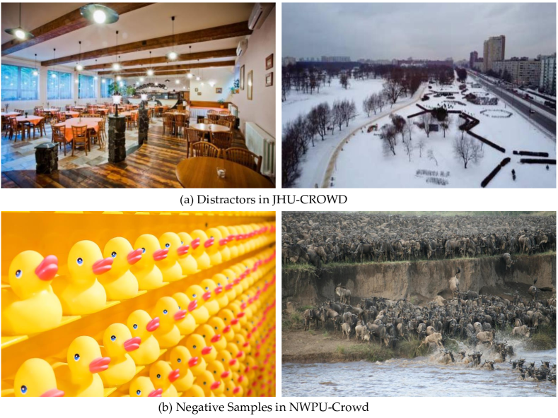
Figure 6: The exemplars of distractors and negative samples for crowd counting.

VI-E Robustness for background

A robust counting model does not only accurately estimate the crowd density but also produce the zero-density response for background regions. To further evaluate models’ robustness, the recently released large-scale datasets, such as JHU-CROWD [134] introduces $100$ distractors and NWPU-Crowd [28] introduces $351$ negative samples into their own datasets, respectively. These data do not contain person objects or crowd regions. It is worth mentioning that NWPU-Crowd [28] deliberately collects some scenes with densely arranged other objects to confuse counting models. Fig. 6 shows some typical distractors and negative samples. These labeled data can effectively facilitate the counting model to perform better in the real world.

TABLE VIII: The MAE/RMSE of mainstream methods on the distractors of JHU-CROWD and the negative samples of NWPU-Crowd.

Method	Distractors in JHU-CROWD	Negative Samples in NWPU-Crowd
MCNN [1]	103.8/238.5	356.0/1232.5
CMTL [1]	135.8/263.8	-
Switching CNN [5]	100.5/235.5	-
SA-Net [11]	71.9/167.7	432.0/974.4
PCC-Net [88]	-	85.3/438.8
CSRNet [12]	44.3/102.4	176.0/572.3
C3F-VGG [211]	-	141.0/474.2
CANNet [86]	-	82.6/343.4
SCAR [210]	-	122.9/660.8
SFCN† [84]	-	54.2/154.7
CG-DRCN [134]	43.4/97.8	-

Table VIII lists the estimation errors (MAE/RMSE) on the aforementioned distractors and negative samples. From the results, we can find that current models mistakenly estimate the density of these samples. For a light model, PCC-Net performs better than many VGG-backbone methods (CSRNet [12], C3F-VGG [211] and SCAR [210]). The main reason may be reside in that PCC-Net [88] incorporates segmentation information to classify the foreground (namely head) and background. Therefore, there maybe an alternative way that uses multi-task learning (patch-level counting, segmentation, group detection, etc.) to extract large-range features.

VI-F Universality or generalization

Nearly all the existing models for object counting are designed for a specific task, however, creating a universal model able to adapt any class of object is a meaningful challenge, it is also the most effective method to evaluate the robustness and generalization ability of the algorithm. Despite there are specialties between different tasks, there still exist many commonalities, such as crowd counting, vehicle counting, and cell counting. For instance, CAC [123] formulates the counting as a matching object through mining the self-similarity between images, which presents a Generic Matching Network (GMN) in a class-agnostic manner. PPPD [124] provides a patch-based, multi-domain object counting network by leveraging a set of domain-specific scaling and normalization layers, which only uses a few of parameters. It can also be extended to perform a visual domain classification even in an unseen observed domain, which outstands out its versatility and modular nature. The method has been successfully applied to people, penguins, and cell counting.

Designing a unified principle (the generation of ground truth density map by using Gaussian function in  [16] takes a good example) and framework that can be applied to different tasks, it looks a bit awkward yet promising research direction in future.

VI-G Lightweight network

Current CNN-based deep models are designed with a sophisticated structure, which always comes with millions of parameters and the cost of a tremendous increase in computation (FLOPs). Although a great effort has been devoted to making the model efficient, such as CSRNet [12] and SCNet [185], they usually adopt VGG16 [205] or ResNet [208] pre-trained on Imagenet [212], which is a large dataset for classification, but the task of object counting belongs to a regression task. Thus it may affect the performance to some extent. Additionally, the pre-trained mechanism is a very time-consuming process. Generally speaking, the most straightforward way to determine whether a network is lightweight is the number of parameters, the less the number of parameters, the lighter of the model. Table IX shows a comparison of the number of parameters in some representative models. From the Table, we can find that LCNN [213] has the least number of parameters, which has nearly 2138 $\times$ lower than the worst one, CP-CNN [6]. We suspect it should be attributed to LCNN [213] is a shallow network without pretraining. Less number of parameters, which proves more efficient of the model.

Lightweight networks can reduce the computation cost, but they are usually accompanied by accuracy drop. Therefore, in the premise of without sacrificing accuracy, designing lightweight and efficient networks to reduce the computation cost in the counting task is a promising challenge in the future.

TABLE IX: Number of parameters (in millions). Red and underline indicate the least and the most parameters’ number, respectively.

Method	Parameters
MCNN [1]	0.13
Hydra-CNN [2]	0.56
Switching CNN [5]	15.11
CP-CNN [6]	68.4
CSRNet [12]	16.26
SA-Net [11]	0.91
ACSCP [74]	5.1
L2R [77]	16.75
DRSAN [71]	24.10
ic-CNN [72]	16.82
IG-CNN [73]	4.70
D-Conv1et [70]	16.62
BSAD [183]	1.30
MMCNN [214]	6.8
TDF-CNN [104]	1.15
ASD [80]	16.26
TEDnet [92]	1.63
ANF [179]	7.9
MRCNet [135]	20.3
SDA-MCNN [215]	2.0
LCNN [213]	0.032

VI-H Combination of image and video

Modern mainstream models for counting have been deployed only for images or videos [216, 217, 19, 218, 213, 162, 219]. When the video sequences are available, some algorithms are proposed to leverage temporal consistency to impel weak constraints on consecutive density estimation. Xiong et al. [217] utilize an LSTM model to estimate densities from one frame to the next. Liu et al. [162] explicitly enforce the constraint under the condition that the number of people must be strictly conserved as they move about. Nevertheless, the constraint is difficult to express, w.r.t. densities. Furthermore, Liu et al. [219] regress people flow rather than regressing densities from video sequences, which imposes strong consistency constraints without complicated network architectures required. Therefore, designing effective algorithms, which can cater to images and videos simultaneous is a meaningful and promising direction.

VI-I Wider-view crowd counting

Albeit outstanding performance have been achieved for crowd counting in single-view images, it is not applicable to large and wide scenes such as public parks or long subway platforms, since it cannot capture sufficient detailed information for a single-view camera. Therefore, to address the problem of wide-area counting, some efforts have been attempted to capture information from multiple camera views. For instance, Zhang et al. [130] proposed a multi-view multi-scale (MVMS) fusion model to predict a 2D scene-level density map on the ground-plane. Furthermore, Zhang et al. [220] achieve this by using 3D feature fusion with 3D scene-level density maps. Compared with 2D fusion [130], 3D fusion not only preserves the property of 2D density maps but also extracts more useful information of the crowd densities along the z-dimension (height). The aforementioned two models are based on the assumption that the cameras are fixed and camera parameters are known, therefore, designing models for cross-scene and multi-view counting with moving cameras and unknown camera parameters is an interesting yet challenging future work.

VI-J Localization, classification and tracking beyond object counting

The density estimation CNN-based models for crowd counting, regression-based methods indeed, although accurate count provided, it does not indicate the precise location and exact size of objects, thus maybe limits the further research and application, such as high-level understanding, localization, classification, and tracking. Some attempts have been made, for instance, DecideNet [7] generates the detection and regression-based density maps separately to estimate crowd density, and an attention module is incorporated to guide the final count. However, the model trains a fully supervised network with bounding box annotations, which needs to take large computation cost. CL [76] regresses density and localization maps simultaneously by introducing a composition loss. LCFCN [221] estimates the crowd count by segmenting the object blobs in an image, which only employs the point-annotations. CL [76] and LCFCN [221] simply concern the localization of crowds, whereas, PSDDN [56] not only predicts the localization but also estimates the size of persons. LSF-CNN [57] locates the position of every person in the crowd, sizes the dot-annotated heads with bounding boxes and finally counts them. All the above works demonstrate that the potential research value of this direction.

VI-K Small or tiny object counting

The problem of small or tiny objects has long been a challenging task in many computer vision communities. In highly congested crowd scenes, the sizes of persons’ heads are tiny. Additionally, some other potential applications may include object counting the number of contiguous dense buildings, ships, small vehicles and countless others in remote sensing images [222]. An apparent difference between object counting in remote sensing scene and nature scenes, the orientations of the objects are arbitrary due to the overhead view rather than upright perspective. Some further directions may include the integration of visual attention mechanism, dilated convolution, deformable convolution layer, and rotation invariance design into the framework.

VII Conclusion

Remarkable progress has been made in crowd counting over the past few decades. This paper has presented a survey of CNN-based density estimation and crowd counting models from several perspectives, including network architecture, learning paradigms, etc. We then summarize popular benchmark datasets, including crowd counting and several representing ones in other fields, as well as evaluation criteria for evaluating various methods. Besides, we also conduct a thorough performance benchmarking evaluation of representative models. Although all the works cannot be covered, we have selected the top-three performers to follow by a comprehensive and thorough analysis and discussion of these representing methods. We summarize the attributes or techniques which have a great assistant for the improvement of the performance.

In the next, we investigate several factors that would affect the performance of crowd counting, and we finally look through some potential challenges and open issues in deep learning era, and put forward insightful discussions and promising research directions in the future.

Standing on the standpoint of technical innovations, we expect this work can provide a feasible scheme to understand state-of-the-art, but more importantly, insights for future exploration in crowd counting and bridge to object counting in other domains.

Guangshuai Gao received the B.Sc. degree in applied physics from college of science and the M.Sc. degree in signal and information processing from the School of Electronic and Information Engineering, from the Zhongyuan University of Technology, Zhengzhou, China, in 2014 and 2017, respectively. He is currently pursuing the Ph.D. degree with the Laboratory of Intelligent Recognition and Image Processing, Beijing Key Laboratory of Digital Media, School of Computer Science and Engineering, Beihang University. His research interests include image processing, pattern recognition, and digital machine learning.

Junyu Gao received the B.E. degree in computer science and technology from the Northwestern Polytechnical University, Xi’an 710072, Shaanxi, P. R. China, in 2015. He is currently pursuing the Ph.D. degree from Center for Optical Imagery Analysis and Learning, Northwestern Polytechnical University, Xian, China. His research interests include computer vision and pattern recognition.

Qingjie Liu received the Ph.D. degree in computer science from the Intelligent Recognition and Image Processing Laboratory, Beihang University, Beijing, China, in 2015. He is currently an Assistant Professor with the School of Computer Science and Engineering, Beihang University. He is also a Distinguished Research Fellow with the Hangzhou Institute of Innovation, Beihang University, Hangzhou. His current research interests include Remote sensing image analysis, pattern recognition, and computer vision. He is a member of the IEEE.

Qi Wang (M’15-SM’15) received the B.E. degree in automation and the Ph.D. degree in pattern recognition and intelligent systems from the University of Science and Technology of China, Hefei, China, in 2005 and 2010, respectively. He is currently a Professor with the School of Computer Science and with the Center for OPTical IMagery Analysis and Learning (OPTIMAL), Northwestern Polytechnical University, Xi’an, China. His research interests include computer vision and pattern recognition.

Yunhong Wang received the B.S. degree in electronic engineering from Northwestern Polytechnical University, Xi’an, China, in 1989, and the M.S. and Ph.D. degrees in electronic engineering from the Nanjing University of Science and Technology, Nanjing, China, in 1995 and 1998, respectively. She was with the National Laboratory of Pattern Recognition, Institute of Automation, Chinese Academy of Sciences, Beijing, China, from 1998 to 2004. Since 2004, she has been a Professor with the School of Computer Science and Engineering, Beihang University, Beijing, where she is also the Director of the Laboratory of Intelligent Recognition and Image Processing and the Beijing Key Laboratory of Digital Media. Her research interests include biometrics, pattern recognition, computer vision, data fusion, and image processing. She is a Fellow of IEEE, IAPR, and CCF.

References

- [1] Y. Zhang, D. Zhou, S. Chen, S. Gao, and Y. Ma, “Single-image crowd counting via multi-column convolutional neural network,” in CVPR, 2016, pp. 589–597.
- [2] D. Onoro-Rubio and R. J. López-Sastre, “Towards perspective-free object counting with deep learning,” in ECCV. Springer, 2016, pp. 615–629.
- [3] L. Boominathan, S. S. Kruthiventi, and R. V. Babu, “Crowdnet: A deep convolutional network for dense crowd counting,” in ACM MM. ACM, 2016, pp. 640–644.
- [4] D. Kang and A. Chan, “Crowd counting by adaptively fusing predictions from an image pyramid,” BMVC, 2018.
- [5] D. B. Sam, S. Surya, and R. V. Babu, “Switching convolutional neural network for crowd counting,” in CVPR. IEEE, 2017, pp. 4031–4039.
- [6] V. A. Sindagi and V. M. Patel, “Generating high-quality crowd density maps using contextual pyramid cnns,” in ICCV, 2017, pp. 1861–1870.
- [7] J. Liu, C. Gao, D. Meng, and A. G. Hauptmann, “Decidenet: Counting varying density crowds through attention guided detection and density estimation,” in CVPR, 2018, pp. 5197–5206.
- [8] M. Hossain, M. Hosseinzadeh, O. Chanda, and Y. Wang, “Crowd counting using scale-aware attention networks,” in WACV. IEEE, 2019, pp. 1280–1288.
- [9] L. Zhang, M. Shi, and Q. Chen, “Crowd counting via scale-adaptive convolutional neural network,” in WACV. IEEE, 2018, pp. 1113–1121.
- [10] J. Sang, W. Wu, H. Luo, H. Xiang, Q. Zhang, H. Hu, and X. Xia, “Improved crowd counting method based on scale-adaptive convolutional neural network,” IEEE Access, 2019.
- [11] X. Cao, Z. Wang, Y. Zhao, and F. Su, “Scale aggregation network for accurate and efficient crowd counting,” in ECCV, 2018, pp. 734–750.
- [12] Y. Li, X. Zhang, and D. Chen, “Csrnet: Dilated convolutional neural networks for understanding the highly congested scenes,” in CVPR, 2018, pp. 1091–1100.
- [13] R. R. Varior, B. Shuai, J. Tighe, and D. Modolo, “Scale-aware attention network for crowd counting,” CVPR, 2019.
- [14] Y. Wang and Y. Zou, “Fast visual object counting via example-based density estimation,” in ICIP. IEEE, 2016, pp. 3653–3657.
- [15] E. Walach and L. Wolf, “Learning to count with cnn boosting,” in ECCV. Springer, 2016, pp. 660–676.
- [16] V. Lempitsky and A. Zisserman, “Learning to count objects in images,” in NIPS, 2010, pp. 1324–1332.
- [17] C. Arteta, V. Lempitsky, and A. Zisserman, “Counting in the wild,” in ECCV. Springer, 2016, pp. 483–498.
- [18] H. Zhang, Z. Kyaw, S.-F. Chang, and T.-S. Chua, “Visual translation embedding network for visual relation detection,” in CVPR, 2017, pp. 5532–5540.
- [19] S. Zhang, G. Wu, J. P. Costeira, and J. M. Moura, “Fcn-rlstm: Deep spatio-temporal neural networks for vehicle counting in city cameras,” in ICCV, 2017, pp. 3667–3676.
- [20] R. Guerrero-Gómez-Olmedo, B. Torre-Jiménez, R. López-Sastre, S. Maldonado-Bascón, and D. Onoro-Rubio, “Extremely overlapping vehicle counting,” in PRIA. Springer, 2015, pp. 423–431.
- [21] S. Aich and I. Stavness, “Leaf counting with deep convolutional and deconvolutional networks,” in ICCV, 2017, pp. 2080–2089.
- [22] M. V. Giuffrida, M. Minervini, and S. A. Tsaftaris, “Learning to count leaves in rosette plants,” 2016.
- [23] G. French, M. Fisher, M. Mackiewicz, and C. Needle, “Convolutional neural networks for counting fish in fisheries surveillance video,” MVAB, pp. 1–7, 2015.
- [24] B. Zhan, D. N. Monekosso, P. Remagnino, S. A. Velastin, and L.-Q. Xu, “Crowd analysis: a survey,” MVA, vol. 19, no. 5-6, pp. 345–357, 2008.
- [25] J. Shao, K. Kang, C. Change Loy, and X. Wang, “Deeply learned attributes for crowded scene understanding,” in CVPR, 2015, pp. 4657–4666.
- [26] B. Zhou, X. Wang, and X. Tang, “Understanding collective crowd behaviors: Learning a mixture model of dynamic pedestrian-agents,” in CVPR. IEEE, 2012, pp. 2871–2878.
- [27] A. B. Chan, Z.-S. J. Liang, and N. Vasconcelos, “Privacy preserving crowd monitoring: Counting people without people models or tracking,” in CVPR. IEEE, 2008, pp. 1–7.
- [28] Q. Wang, J. Gao, W. Lin, and X. Li, “Nwpu-crowd: A large-scale benchmark for crowd counting,” arXiv:2001.03360v1, 2020.
- [29] I. S. Topkaya, H. Erdogan, and F. Porikli, “Counting people by clustering person detector outputs,” in AVSS. IEEE, 2014, pp. 313–318.
- [30] M. Li, Z. Zhang, K. Huang, and T. Tan, “Estimating the number of people in crowded scenes by mid based foreground segmentation and head-shoulder detection,” in ICPR. IEEE, 2008, pp. 1–4.
- [31] B. Leibe, E. Seemann, and B. Schiele, “Pedestrian detection in crowded scenes,” in CVPR, vol. 1. IEEE, 2005, pp. 878–885.
- [32] M. Enzweiler and D. M. Gavrila, “Monocular pedestrian detection: Survey and experiments,” TPAMI, vol. 31, no. 12, pp. 2179–2195, 2009.
- [33] R. Girshick, “Fast r-cnn,” in ICCV, 2015, pp. 1440–1448.
- [34] S. Ren, K. He, R. Girshick, and J. Sun, “Faster r-cnn: Towards real-time object detection with region proposal networks,” in NIPS, 2015, pp. 91–99.
- [35] K. He, G. Gkioxari, P. Dollár, and R. Girshick, “Mask r-cnn,” in ICCV, 2017, pp. 2961–2969.
- [36] J. Redmon, S. Divvala, R. Girshick, and A. Farhadi, “You only look once: Unified, real-time object detection,” in CVPR, 2016, pp. 779–788.
- [37] W. Liu, D. Anguelov, D. Erhan, C. Szegedy, S. Reed, C.-Y. Fu, and A. C. Berg, “Ssd: Single shot multibox detector,” in ECCV. Springer, 2016, pp. 21–37.
- [38] H. Idrees, I. Saleemi, C. Seibert, and M. Shah, “Multi-source multi-scale counting in extremely dense crowd images,” in CVPR, 2013, pp. 2547–2554.
- [39] A. B. Chan and N. Vasconcelos, “Bayesian poisson regression for crowd counting,” in ICCV. IEEE, 2009, pp. 545–551.
- [40] K. Chen, C. C. Loy, S. Gong, and T. Xiang, “Feature mining for localised crowd counting.” in BMVC, vol. 1, no. 2, 2012, p. 3.
- [41] D. Ryan, S. Denman, C. Fookes, and S. Sridharan, “Crowd counting using multiple local features,” in DITCA. IEEE, 2009, pp. 81–88.
- [42] D. G. Lowe et al., “Object recognition from local scale-invariant features.” in ICCV, vol. 99, no. 2, 1999, pp. 1150–1157.
- [43] T. Ojala, M. Pietikäinen, and T. Mäenpää, “Gray scale and rotation invariant texture classification with local binary patterns,” in ECCV. Springer, 2000, pp. 404–420.
- [44] N. Dalal and B. Triggs, “Histograms of oriented gradients for human detection,” in CVPR, vol. 1. IEEE Computer Society, 2005, pp. 886–893.
- [45] R. M. Haralick, K. Shanmugam et al., “Textural features for image classification,” TSMC, no. 6, pp. 610–621, 1973.
- [46] N. Paragios and V. Ramesh, “A mrf-based approach for real-time subway monitoring,” in CVPR, vol. 1. IEEE, 2001, pp. 1–1034.
- [47] Y. Tian, L. Sigal, H. Badino, F. De la Torre, and Y. Liu, “Latent gaussian mixture regression for human pose estimation,” in ACCV. Springer, 2010, pp. 679–690.
- [48] V.-Q. Pham, T. Kozakaya, O. Yamaguchi, and R. Okada, “Count forest: Co-voting uncertain number of targets using random forest for crowd density estimation,” in ICCV, 2015, pp. 3253–3261.
- [49] C. Wang, H. Zhang, L. Yang, S. Liu, and X. Cao, “Deep people counting in extremely dense crowds,” in ACM MM. ACM, 2015, pp. 1299–1302.
- [50] M. Fu, P. Xu, X. Li, Q. Liu, M. Ye, and C. Zhu, “Fast crowd density estimation with convolutional neural networks,” EAAI, vol. 43, pp. 81–88, 2015.
- [51] C. Zhang, H. Li, X. Wang, and X. Yang, “Cross-scene crowd counting via deep convolutional neural networks,” in CVPR, 2015, pp. 833–841.
- [52] X. Wu, G. Liang, K. K. Lee, and Y. Xu, “Crowd density estimation using texture analysis and learning,” in ICRB. IEEE, 2006, pp. 214–219.
- [53] S. An, W. Liu, and S. Venkatesh, “Face recognition using kernel ridge regression,” in CVPR. IEEE, 2007, pp. 1–7.
- [54] K. Chen, S. Gong, T. Xiang, and C. Change Loy, “Cumulative attribute space for age and crowd density estimation,” in CVPR, 2013, pp. 2467–2474.
- [55] V. A. Sindagi and V. M. Patel, “Cnn-based cascaded multi-task learning of high-level prior and density estimation for crowd counting,” in AVSS. IEEE, 2017, pp. 1–6.
- [56] Y. Liu, M. Shi, Q. Zhao, and X. Wang, “Point in, box out: Beyond counting persons in crowds,” CVPR, 2019.
- [57] D. B. Sam, S. V. Peri, A. Kamath, R. V. Babu et al., “Locate, size and count: Accurately resolving people in dense crowds via detection,” arXiv preprint arXiv:1906.07538, 2019.
- [58] J. C. S. J. Junior, S. R. Musse, and C. R. Jung, “Crowd analysis using computer vision techniques,” ISPM, vol. 27, no. 5, pp. 66–77, 2010.
- [59] T. Teixeira, G. Dublon, and A. Savvides, “A survey of human-sensing: Methods for detecting presence, count, location, track, and identity,” ACM Computing Surveys, vol. 5, no. 1, pp. 59–69, 2010.
- [60] C. C. Loy, K. Chen, S. Gong, and T. Xiang, “Crowd counting and profiling: Methodology and evaluation,” in MSVAC. Springer, 2013, pp. 347–382.
- [61] J. Ferryman and A.-L. Ellis, “Performance evaluation of crowd image analysis using the pets2009 dataset,” PRL, vol. 44, pp. 3–15, 2014.
- [62] T. Li, H. Chang, M. Wang, B. Ni, R. Hong, and S. Yan, “Crowded scene analysis: A survey,” TCSVT, vol. 25, no. 3, pp. 367–386, 2015.
- [63] D. Ryan, S. Denman, S. Sridharan, and C. Fookes, “An evaluation of crowd counting methods, features and regression models,” CVIU, vol. 130, pp. 1–17, 2015.
- [64] S. A. M. Saleh, S. A. Suandi, and H. Ibrahim, “Recent survey on crowd density estimation and counting for visual surveillance,” EAAI, vol. 41, pp. 103–114, 2015.
- [65] M. S. Zitouni, H. Bhaskar, J. Dias, and M. E. Al-Mualla, “Advances and trends in visual crowd analysis: A systematic survey and evaluation of crowd modelling techniques,” Neurocomputing, vol. 186, pp. 139–159, 2016.
- [66] J. M. Grant and P. J. Flynn, “Crowd scene understanding from video: a survey,” TOMM, vol. 13, no. 2, p. 19, 2017.
- [67] V. A. Sindagi and V. M. Patel, “A survey of recent advances in cnn-based single image crowd counting and density estimation,” PRL, vol. 107, pp. 3–16, 2018.
- [68] G. Tripathi, K. Singh, and D. K. Vishwakarma, “Convolutional neural networks for crowd behaviour analysis: a survey,” The Visual Computer, vol. 35, no. 5, pp. 753–776, 2019.
- [69] C. Shang, H. Ai, and B. Bai, “End-to-end crowd counting via joint learning local and global count,” in ICIP. IEEE, 2016, pp. 1215–1219.
- [70] Z. Shi, L. Zhang, Y. Liu, X. Cao, Y. Ye, M.-M. Cheng, and G. Zheng, “Crowd counting with deep negative correlation learning,” in CVPR, 2018, pp. 5382–5390.
- [71] L. Liu, H. Wang, G. L. andWanli Ouyang, and L. Lin, “Crowd counting using deep recurrent spatial-aware network,” in IJCAI, 2018, pp. 849–855.
- [72] D. Babu Sam, N. N. Sajjan, R. Venkatesh Babu, and M. Srinivasan, “Divide and grow: capturing huge diversity in crowd images with incrementally growing cnn,” in CVPR, 2018, pp. 3618–3626.
- [73] V. Ranjan, H. Le, and M. Hoai, “Iterative crowd counting,” in ECCV, 2018, pp. 270–285.
- [74] Z. Shen, Y. Xu, B. Ni, M. Wang, J. Hu, and X. Yang, “Crowd counting via adversarial cross-scale consistency pursuit,” in CVPR, 2018, pp. 5245–5254.
- [75] Z. Shi, L. Zhang, Y. Sun, and Y. Ye, “Multiscale multitask deep netvlad for crowd counting,” TII, vol. 14, no. 11, pp. 4953–4962, 2018.
- [76] H. Idrees, M. Tayyab, K. Athrey, D. Zhang, S. Al-Maadeed, N. Rajpoot, and M. Shah, “Composition loss for counting, density map estimation and localization in dense crowds,” in ECCV, 2018, pp. 532–546.
- [77] X. Liu, J. van de Weijer, and A. D. Bagdanov, “Leveraging unlabeled data for crowd counting by learning to rank,” in CVPR, 2018, pp. 7661–7669.
- [78] G. Olmschenk, H. Tang, and Z. Zhu, “Crowd counting with minimal data using generative adversarial networks for multiple target regression,” in WACV. IEEE, 2018, pp. 1151–1159.
- [79] Y. Tian, Y. Lei, J. Zhang, and J. Z. Wang, “Padnet: Pan-density crowd counting,” TIP, 2019.
- [80] X. Wu, Y. Zheng, H. Ye, W. Hu, J. Yang, and L. He, “Adaptive scenario discovery for crowd counting,” ICASSP, 2019.
- [81] C. X., B. Y., S. N., and G. C., “Scale pyramid network for crowd counting,” in WACV, 2019, pp. 1941–1950.
- [82] G. Olmschenk, Z. Zhu, and H. Tang, “Generalizing semi-supervised generative adversarial networks to regression using feature contrasting,” CVIU, vol. 186, pp. 1–12, 2019.
- [83] N. Liu, Y. Long, C. Zou, Q. Niu, L. Pan, and H. Wu, “Adcrowdnet: An attention-injective deformable convolutional network for crowd understanding,” CVPR, 2019.
- [84] Q. Wang, J. Gao, W. Lin, and Y. Yuan, “Learning from synthetic data for crowd counting in the wild,” in CVPR, 2019.
- [85] M. Shi, Z. Yang, C. Xu, and Q. Chen, “Revisiting perspective information for efficient crowd counting,” CVPR, 2019.
- [86] W. Liu, M. Salzmann, and P. Fua, “Context-aware crowd counting,” CVPR, 2019.
- [87] P. M. Zenglin Shi and C. G. M. Snoek, “Counting with focus for free,” in ICCV, 2019, pp. 4200–4209.
- [88] J. Gao, Q. Wang, and X. Li, “Pcc net: Perspective crowd counting via spatial convolutional network,” TCSVT, 2019.
- [89] L. Zhu, Z. Zhao, C. Lu, Y. Lin, Y. Peng, and T. Yao, “Dual path multi-scale fusion networks with attention for crowd counting,” arXiv preprint arXiv:1902.01115, 2019.
- [90] V. K. Valloli and K. Mehta, “W-net: Reinforced u-net for density map estimation,” arXiv preprint arXiv:1903.11249, 2019.
- [91] X. Liu, J. Van De Weijer, and A. D. Bagdanov, “Exploiting unlabeled data in cnns by self-supervised learning to rank,” TPAMI, 2019.
- [92] X. Jiang, Z. Xiao, B. Zhang, X. Zhen, X. Cao, D. Doermann, and L. Shao, “Crowd counting and density estimation by trellis encoder-decoder network,” CVPR, 2019.
- [93] J. Wan, W. Luo, B. Wu, A. B. Chan, and W. Liu, “Residual regression with semantic prior for crowd counting,” in CVPR, 2019, pp. 4036–4045.
- [94] C. Liu, X. Weng, and Y. Mu, “Recurrent attentive zooming for joint crowd counting and precise localization,” in CVPR, 2019, pp. 1217–1226.
- [95] M. Zhao, J. Zhang, C. Zhang, and W. Zhang, “Leveraging heterogeneous auxiliary tasks to assist crowd counting,” in CVPR, 2019, pp. 12 736–12 745.
- [96] H. M. R. V. B. Deepak Babu Sam, Neeraj N Sajjan, “Almost unsupervised learning for dense crowd counting,” in AAAI, 2019.
- [97] V. A. Sindagi and V. M. Patel, “Ha-ccn: Hierarchical attention-based crowd counting network,” TIP, 2019.
- [98] C. Xu, K. Qiu, J. Fu, S. Bai, Y. Xu, and X. Bai, “Learn to scale: Generating multipolar normalized density map for crowd counting,” in ICCV, 2019.
- [99] A. Zhang, J. Shen, Z. Xiao, F. Zhu, X. Zhen, X. Cao, and L. Shao, “Relational attention network for crowd counting,” in ICCV, 2019, pp. 6788–6797.
- [100] Z. Cheng, J. Li, D. Qi, W. Xiao, H. Junyan, and H. Alexander, “Improving the learning of multi-column convolutional neural network for crowd counting,” ACMMM, 2019.
- [101] H. Cholakkal, G. Sun, F. S. Khan, and L. Shao, “Object counting and instance segmentation with image-level supervision,” CVPR, 2019.
- [102] A. Krizhevsky, I. Sutskever, and G. E. Hinton, “Imagenet classification with deep convolutional neural networks,” in NIPS, 2012, pp. 1097–1105.
- [103] I. Goodfellow, J. Pouget-Abadie, M. Mirza, B. Xu, D. Warde-Farley, S. Ozair, A. Courville, and Y. Bengio, “Generative adversarial nets,” in NIPS, 2014, pp. 2672–2680.
- [104] D. B. Sam and R. V. Babu, “Top-down feedback for crowd counting convolutional neural network,” in AAAI, 2018.
- [105] M. Jaderberg, K. Simonyan, A. Zisserman et al., “Spatial transformer networks,” in NIPS, 2015, pp. 2017–2025.
- [106] S. Kumagai, K. Hotta, and T. Kurita, “Mixture of counting cnns: Adaptive integration of cnns specialized to specific appearance for crowd counting,” arXiv preprint arXiv:1703.09393, 2017.
- [107] D. Guo, K. Li, Z.-J. Zha, and M. Wang, “Dadnet: Dilated-attention-deformable convnet for crowd counting,” in ACMMM. ACM, 2019, pp. 1823–1832.
- [108] B. Sheng, C. Shen, G. Lin, J. Li, W. Yang, and C. Sun, “Crowd counting via weighted vlad on dense attribute feature maps,” TCSVT, vol. 28, no. 8, pp. 1788–1797, 2018.
- [109] C. Szegedy, W. Liu, Y. Jia, P. Sermanet, S. Reed, D. Anguelov, D. Erhan, V. Vanhoucke, and A. Rabinovich, “Going deeper with convolutions,” in CVPR, 2015, pp. 1–9.
- [110] O. Ronneberger, P. Fischer, and T. Brox, “U-net: Convolutional networks for biomedical image segmentation,” in ICMICCAI. Springer, 2015, pp. 234–241.
- [111] R. Caruana, “Multitask learning,” Machine learning, vol. 28, no. 1, pp. 41–75, 1997.
- [112] D. Kang, Z. Ma, and A. B. Chan, “Beyond counting: Comparisons of density maps for crowd analysis tasks-counting, detection, and tracking,” TCSVT, 2018.
- [113] L. Zhang, Z. Shi, M.-M. Cheng, Y. Liu, J.-W. Bian, J. T. Zhou, G. Zheng, and Z. Zeng, “Nonlinear regression via deep negative correlation learning,” TPAMI, 2019.
- [114] Q. Wang, J. Wan, and Y. Yuan, “Deep metric learning for crowdedness regression,” TCSVT, vol. 28, no. 10, pp. 2633–2643, 2018.
- [115] C. Xu, D. Liang, Y. Xu, W. Zhan, M. Tomizuka, and X. Bai, “Autoscale: Learning to scale for crowd counting,” arXiv:1912.09632, 2019.
- [116] S. Aich and I. Stavness, “Global sum pooling: A generalization trick for object counting with small datasets of large images,” in CVPRW, 2019, pp. 73–82.
- [117] B. Sheng, C. Shen, G. Lin, J. Li, W. Yang, and C. Sun, “Crowd counting via weighted vlad on a dense attribute feature map,” TCSVT, vol. 28, no. 8, pp. 1788–1797, 2016.
- [118] A. Makhzani and B. J. Frey, “Winner-take-all autoencoders,” in NIPS, 2015, pp. 2791–2799.
- [119] G. Olmschenk, J. Chen, H. Tang, and Z. Zhu, “Dense crowd counting convolutional neural networks with minimal data using semi-supervised dual-goal generative adversarial networks,” in CVPRW, 2019, pp. 21–28.
- [120] Q. Zhou, J. Zhang, L. Che, H. Shan, and J. Z. Wang, “Crowd counting with limited labeling through submodular frame selection,” T-ITS, vol. 20, no. 5, pp. 1728–1738, 2018.
- [121] L. Wang, Y. Li, and X. Xue, “Coda: Counting objects via scale-aware adversarial density adaption,” ICME, 2019.
- [122] M. A. Hossain, M. Kumar, M. Hosseinzadeh, O. Chanda, and Y. Wang, “One-shot scene-specific crowd counting,” BMVC, 2019.
- [123] E. Lu, W. Xie, and A. Zisserman, “Class-agnostic counting,” ACCV, 2018.
- [124] M. Marsden, K. McGuinness, S. Little, C. E. Keogh, and N. E. O’Connor, “People, penguins and petri dishes: Adapting object counting models to new visual domains and object types without forgetting,” in CVPR, 2018, pp. 8070–8079.
- [125] Z. Wang, A. C. Bovik, H. R. Sheikh, E. P. Simoncelli et al., “Image quality assessment: from error visibility to structural similarity,” TIP, vol. 13, no. 4, pp. 600–612, 2004.
- [126] J. Gao, Q. Wang, and Y. Yuan, “Feature-aware adaptation and structured density alignment for crowd counting in video surveillance,” arXiv:1912.03672, 2019.
- [127] J. Gao, T. Han, Q. Wang, and Y. Yuan, “Domain-adaptive crowd counting via inter-domain features segregation and gaussian-prior reconstruction,” arXiv:1912.03677, 2019.
- [128] T. Han, J. Gao, Y. Yuan, and W. Qi, “Focus on semantic consistency for cross-domain crowd understanding,” arXiv preprint arXiv:2002.08623, 2020.
- [129] P. Chattopadhyay, R. Vedantam, R. R. Selvaraju, D. Batra, and D. Parikh, “Counting everyday objects in everyday scenes,” in CVPR, 2017, pp. 1135–1144.
- [130] Q. Zhang and A. B. Chan, “Wide-area crowd counting via ground-plane density maps and multi-view fusion cnns,” in CVPR, 2019, pp. 8297–8306.
- [131] D. Lian, J. Li, J. Zheng, W. Luo, and S. Gao, “Density map regression guided detection network for rgb-d crowd counting and localization,” in CVPR, 2019, pp. 1821–1830.
- [132] Y. Fang, B. Zhan, W. Cai, S. Gao, and B. Hu, “Locality-constrained spatial transformer network for video crowd counting,” in ICME. IEEE, 2019, pp. 814–819.
- [133] Z. Yan, Y. Yuan, W. Zuo, T. Xiao, Y. Wang, S. Wen, and E. Ding, “Perspective-guided convolution networks for crowd counting,” in ICCV, 2019.
- [134] V. A. Sindagi, R. Yasarla, and V. M. Patel, “Pushing the frontiers of unconstrained crowd counting: New dataset and benchmark method,” in ICCV, 2019, pp. 1221–1231.
- [135] R. Bahmanyar, E. Vig, and P. Reinartz, “Mrcnet: Crowd counting and density map estimation in aerial and ground imagery,” BMVCW, 2019.
- [136] L. Wen, D. Du, P. Zhu, Q. Hu, Q. Wang, L. Bo, and S. Lyu, “Drone-based joint density map estimation, localization and tracking with space-time multi-scale attention network,” arXiv:1912.01811, 2019.
- [137] B. Yao, X. Yang, and S.-C. Zhu, “Introduction to a large-scale general purpose ground truth database: methodology, annotation tool and benchmarks,” in EMMCVPRW. Springer, 2007, pp. 169–183.
- [138] A. Ellis and J. Ferryman, “Pets2010: Dataset and challenge,” AVSS, pp. 143–150, 2010.
- [139] M. K. Lim, V. J. Kok, C. C. Loy, and C. S. Chan, “Crowd saliency detection via global similarity structure,” in ICPR. IEEE, 2014, pp. 3957–3962.
- [140] E. Bondi, L. Seidenari, A. D. Bagdanov, and A. Del Bimbo, “Real-time people counting from depth imagery of crowded environments,” in AVSS. IEEE, 2014, pp. 337–342.
- [141] J. Luo, J. Wang, H. Xu, and H. Lu, “Real-time people counting for indoor scenes,” Signal Processing, vol. 124, pp. 27–35, 2016.
- [142] Z. Zhao, H. Li, R. Zhao, and X. Wang, “Crossing-line crowd counting with two-phase deep neural networks,” in ECCV. Springer, 2016, pp. 712–726.
- [143] Y. Hu, H. Chang, F. Nian, Y. Wang, and T. Li, “Dense crowd counting from still images with convolutional neural networks,” VCIR, vol. 38, pp. 530–539, 2016.
- [144] H. Farhood, X. He, W. Jia, M. Blumenstein, and H. Li, “Counting people based on linear, weighted, and local random forests,” in DICTA. IEEE, 2017, pp. 1–7.
- [145] G. He, Q. Chen, D. Jiang, X. Lu, and Y. Yuan, “A double-region learning algorithm for counting the number of pedestrians in subway surveillance videos,” EAAI, vol. 64, pp. 302–314, 2017.
- [146] X. Ding, Z. Lin, F. He, Y. Wang, and Y. Huang, “A deeply-recursive convolutional network for crowd counting,” in ICASSP. IEEE, 2018, pp. 1942–1946.
- [147] H. Zheng, Z. Lin, J. Cen, Z. Wu, and Y. Zhao, “Cross-line pedestrian counting based on spatially-consistent two-stage local crowd density estimation and accumulation,” T-CSVT, vol. 29, no. 3, pp. 787–799, 2018.
- [148] G. Schröder, T. Senst, E. Bochinski, and T. Sikora, “Optical flow dataset and benchmark for visual crowd analysis,” in AVSS. IEEE, 2018, pp. 1–6.
- [149] M. Xu, Z. Ge, X. Jiang, G. Cui, B. Zhou, C. Xu et al., “Depth information guided crowd counting for complex crowd scenes,” PRL, 2019.
- [150] M. Ling and X. Geng, “Indoor crowd counting by mixture of gaussians label distribution learning,” TIP, vol. 28, no. 11, pp. 5691–5701, 2019.
- [151] X. Jiang, L. Zhang, P. Lv, Y. Guo, R. Zhu, Y. Li, Y. Pang, X. Li, B. Zhou, and M. Xu, “Learning multi-level density maps for crowd counting.” T-NNLS, 2019.
- [152] S. S. S. Das, S. M. Rashid, M. E. Ali et al., “Cccnet: An attention based deep learning framework for categorized crowd counting,” arXiv preprint arXiv:1912.05765, 2019.
- [153] P. Dollar, C. Wojek, B. Schiele, and P. Perona, “Pedestrian detection: An evaluation of the state of the art,” TPAMI, vol. 34, no. 4, pp. 743–761, 2012.
- [154] S. Yang, P. Luo, C.-C. Loy, and X. Tang, “Wider face: A face detection benchmark,” in CVPR, 2016, pp. 5525–5533.
- [155] E. Ristani, F. Solera, R. Zou, R. Cucchiara, and C. Tomasi, “Performance measures and a data set for multi-target, multi-camera tracking,” in ECCV. Springer, 2016, pp. 17–35.
- [156] S. Zhang, G. Wu, J. P. Costeira, and J. M. Moura, “Understanding traffic density from large-scale web camera data,” in Proceedings of the IEEE Conference on Computer Vision and Pattern Recognition, 2017, pp. 5898–5907.
- [157] M.-R. Hsieh, Y.-L. Lin, and W. H. Hsu, “Drone-based object counting by spatially regularized regional proposal network,” in ICCV, 2017, pp. 4145–4153.
- [158] H. Lu, Z. Cao, Y. Xiao, B. Zhuang, and C. Shen, “Tasselnet: counting maize tassels in the wild via local counts regression network,” Plant methods, vol. 13, no. 1, p. 79, 2017.
- [159] A. Josuttes, S. Aich, I. Stavness, C. Pozniak, and S. Shirtliffe, “Utilizing deep learning to predict the number of spikes in wheat (triticum aestivum),” Phenome 2018 Posters, vol. 5, p. 8, 2018.
- [160] P. Zhu, L. Wen, X. Bian, H. Ling, and Q. Hu, “Vision meets drones: A challenge,” arXiv preprint arXiv:1804.07437, 2018.
- [161] H. Bai, S. Wen, and S.-H. G. Chan, “Crowd counting on images with scale variation and isolated clusters,” ICCVW, 2019.
- [162] W. Liu, K. M. Lis, M. Salzmann, and P. Fua, “Geometric and physical constraints for drone-based head plane crowd density estimation,” in IROS, 2019.
- [163] F. Dai, H. Liu, Y. Ma, J. Cao, Q. Zhao, and Y. Zhang, “Dense scale network for crowd counting,” CoRR, vol. abs/1906.09707, 2019.
- [164] J. Hu, L. Shen, and G. Sun, “Squeeze-and-excitation networks,” in CVPR, 2018, pp. 7132–7141.
- [165] M. Ren and R. S. Zemel, “End-to-end instance segmentation with recurrent attention,” in CVPR, 2017, pp. 6656–6664.
- [166] R. Qian, R. T. Tan, W. Yang, J. Su, and J. Liu, “Attentive generative adversarial network for raindrop removal from a single image,” in CVPR, 2018, pp. 2482–2491.
- [167] X. Chu, W. Yang, W. Ouyang, C. Ma, A. L. Yuille, and X. Wang, “Multi-context attention for human pose estimation,” in CVPR, 2017, pp. 1831–1840.
- [168] F. Yu and V. Koltun, “Multi-scale context aggregation by dilated convolutions,” arXiv preprint arXiv:1511.07122, 2015.
- [169] L.-C. Chen, G. Papandreou, I. Kokkinos, K. Murphy, and A. L. Yuille, “Deeplab: Semantic image segmentation with deep convolutional nets, atrous convolution, and fully connected crfs,” TPAMI, vol. 40, no. 4, pp. 834–848, 2018.
- [170] L.-C. Chen, G. Papandreou, F. Schroff, and H. Adam, “Rethinking atrous convolution for semantic image segmentation,” arXiv preprint arXiv:1706.05587, 2017.
- [171] J. Long, E. Shelhamer, and T. Darrell, “Fully convolutional networks for semantic segmentation,” in CVPR, 2015, pp. 3431–3440.
- [172] J. Dai, H. Qi, Y. Xiong, Y. Li, G. Zhang, H. Hu, and Y. Wei, “Deformable convolutional networks,” in ICCV, 2017, pp. 764–773.
- [173] Z. Wang, T. Chen, G. Li, R. Xu, and L. Lin, “Multi-label image recognition by recurrently discovering attentional regions,” in ICCV, 2017, pp. 464–472.
- [174] J. Kuen, Z. Wang, and G. Wang, “Recurrent attentional networks for saliency detection,” in CVPR, 2016, pp. 3668–3677.
- [175] J. Lafferty, A. McCallum, and F. C. Pereira, “Conditional random fields: Probabilistic models for segmenting and labeling sequence data,” 2001.
- [176] S. Z. Li, “Markov random field models in computer vision,” in European conference on computer vision. Springer, 1994, pp. 361–370.
- [177] P. Krähenbühl and V. Koltun, “Efficient inference in fully connected crfs with gaussian edge potentials,” in NIPS, 2011, pp. 109–117.
- [178] L. Liu, Z. Qiu, G. Li, S. Liu, W. Ouyang, and L. Lin, “Crowd counting with deep structured scale integration network,” in ICCV, 2019.
- [179] A. Zhang, L. Yue, J. Shen, F. Zhu, X. Zhen, X. Cao, and L. Shao, “Attentional neural fields for crowd counting,” in ICCV, 2019, pp. 5714–5713.
- [180] X. Wang, R. Girshick, A. Gupta, and K. He, “Non-local neural networks,” in CVPR, 2018, pp. 7794–7803.
- [181] X.-S. Gao, X.-R. Hou, J. Tang, and H.-F. Cheng, “Complete solution classification for the perspective-three-point problem,” TPAMI, vol. 25, no. 8, pp. 930–943, 2003.
- [182] A. B. Chan and N. Vasconcelos, “Counting people with low-level features and bayesian regression,” TIP, vol. 21, no. 4, pp. 2160–2177, 2012.
- [183] S. Huang, X. Li, Z. Zhang, F. Wu, S. Gao, R. Ji, and J. Han, “Body structure aware deep crowd counting,” TIP, vol. 27, no. 3, pp. 1049–1059, 2018.
- [184] K. He, X. Zhang, S. Ren, and J. Sun, “Spatial pyramid pooling in deep convolutional networks for visual recognition,” TPAMI, vol. 37, no. 9, pp. 1904–1916, 2015.
- [185] Z. Wang, Z. Xiao, K. Xie, Q. Qiu, X. Zhen, and X. Cao, “In defense of single-column networks for crowd counting,” arXiv preprint arXiv:1808.06133, 2018.
- [186] L. Zeng, X. Xu, B. Cai, S. Qiu, and T. Zhang, “Multi-scale convolutional neural networks for crowd counting,” in ICIP. IEEE, 2017, pp. 465–469.
- [187] S. Jiang, X. Lu, Y. Lei, and L. Liu, “Mask-aware networks for crowd counting,” TCSVT, 2019.
- [188] M.-h. Oh, P. A. Olsen, and K. N. Ramamurthy, “Crowd counting with decomposed uncertainty,” AAAI, 2019.
- [189] R. Viresh, S. Mubarak, and H. N. Minh, “Crowd transformer network,” arXiv preprint arXiv:1904.02774v1, 2019.
- [190] L. Liu, J. Jiang, W. Jia, S. Amirgholipour, M. Zeibots, and X. He, “Denet: A universal network for counting crowd with varying densities and scales,” Neurocomputing, 2019.
- [191] V. A. Sindagi and V. M. Patel, “Inverse attention guided deep crowd counting network,” AVSS, 2019.
- [192] Z. Ma, X. Wei, X. Hong, and Y. Gong, “Bayesian loss for crowd count estimation with point supervision,” in ICCV, 2019, pp. 6142–6151.
- [193] Z.-Q. Cheng, J.-X. Li, Q. Dai, X. Wu, and A. G. Hauptmann, “Learning spatial awareness to improve crowd counting,” ICCV, 2019.
- [194] V. A. Sindagi and V. M. Patel, “Multi-level bottom-top and top-bottom feature fusion for crowd counting,” ICCV, 2019.
- [195] H. Xiong, H. Lu, C. Liu, L. Liang, Z. Cao, and C. Shen, “From open set to closed set: Counting objects by spatial divide-and-conquer,” in ICCV, 2019.
- [196] J. Ma, Y. Dai, and Y.-P. Tan, “Atrous convolutions spatial pyramid network for crowd counting and density estimation.” Neurocomputing, vol. 350, pp. 91–101, 2019.
- [197] J. Chen, S. Wen, and Z. Wang, “Crowd counting with crowd attention convolutional neural network,” Neurocomputing, 2019.
- [198] X. Tan, C. Tao, T. R. andJinhui Tang, and G. Wu, “Crowd counting via multi-layer regression,” in ACMMM. ACM, 2019, pp. 1907–1915.
- [199] M. M. Oghaz, A. R. Khadka, V. Argyriou, and P. Remagnino, “Content-aware density map for crowd counting and density estimation,” arXiv preprint arXiv:1906.07258, 2019.
- [200] G. Olmschenk, H. Tang, and Z. Zhu, “Improving dense crowd counting convolutional neural networks using inverse k-nearest neighbor maps and multiscale upsampling,” arXiv preprint arXiv:1902.05379, 2019.
- [201] J. Wan and A. Chan, “Adaptive density map generation for crowd counting,” in ICCV, 2019, pp. 1130–1139.
- [202] V. Belagiannis, C. Rupprecht, G. Carneiro, and N. Navab, “Robust optimization for deep regression,” in ICCV, 2015, pp. 2830–2838.
- [203] J. Yang, Y. Zhou, and S.-Y. Kung, “Multi-scale generative adversarial networks for crowd counting,” in ICPR. IEEE, 2018, pp. 3244–3249.
- [204] Z. Qiu, L. Liu, G. Li, Q. Wang, N. Xiao, and L. Lin, “Crowd counting via multi-view scale aggregation networks,” in ICME. IEEE, 2019, pp. 1498–1503.
- [205] K. Simonyan and A. Zisserman, “Very deep convolutional networks for large-scale image recognition,” arXiv preprint arXiv:1409.1556, 2014.
- [206] Q. Wang and T. P. Breckon, “Segmentation guided attention network for crowd counting via curriculum learning,” arXiv preprint arXiv:1911.07990, 2019.
- [207] C. Szegedy, V. Vanhoucke, S. Ioffe, J. Shlens, and Z. Wojna, “Rethinking the inception architecture for computer vision,” in CVPR, 2016, pp. 2818–2826.
- [208] K. He, X. Zhang, S. Ren, and J. Sun, “Deep residual learning for image recognition,” in CVPR, 2016, pp. 770–778.
- [209] H. Jiang and W. Jin, “Effective use of convolutional neural networks and diverse deep supervision for better crowd counting,” Applied Intelligence, pp. 1–19, 2019.
- [210] J. Gao, Q. Wang, and Y. Yuan, “Scar: Spatial-/channel-wise attention regression networks for crowd counting,” Neurocomputing, vol. 363, pp. 1–8, 2019.
- [211] J. Gao, W. Lin, B. Zhao, D. Wang, C. Gao, and J. Wen, “C3 framework: An open-source pytorch code for crowd counting,” arXiv preprint arXiv:1907.02724, 2019.
- [212] J. Deng, W. Dong, R. Socher, L.-J. Li, K. Li, and L. Fei-Fei, “Imagenet: A large-scale hierarchical image database,” in CVPR. IEEE, 2009, pp. 248–255.
- [213] X. Wu, B. Xu, Y. Zheng, H. Ye, J. Yang, and L. He, “Video crowd counting via dynamic temporal modeling,” arXiv preprint arXiv:1907.02198, 2019.
- [214] B. Yang, J. Cao, N. Wang, Y. Zhang, and L. Zou, “Counting challenging crowds robustly using a multi-column multi-task convolutional neural network,” SPIC, vol. 64, pp. 118–129, 2018.
- [215] B. Yang, W. Zhan, N. Wang, X. Liu, and J. Lv, “Counting crowds using a scale-distribution-aware network and adaptive human-shaped kernel,” Neurocomputing, 2019.
- [216] Z. Zou, H. Shao, X. Qu, W. Wei, and P. Zhou, “Enhanced 3d convolutional networks for crowd counting,” BMVC, 2019.
- [217] F. Xiong, X. Shi, and D.-Y. Yeung, “Spatiotemporal modeling for crowd counting in videos,” in ICCV, 2017, pp. 5151–5159.
- [218] G. He, Z. Ma, B. Huang, B. Sheng, and Y. Yuan, “Dynamic region division for adaptive learning pedestrian counting,” in ICME. IEEE, 2019, pp. 1120–1125.
- [219] W. Liu, M. Salzmann, and P. Fua, “Estimating people flows to better count them in crowded scenes,” arXiv preprint arXiv:1911.10782, 2019.
- [220] Q. Zhang and A. B. Chan, “3d crowd counting via multi-view fusion with 3d gaussian kernels,” in AAAI, 2020.
- [221] I. H. Laradji, N. Rostamzadeh, P. O. Pinheiro, D. Vazquez, and M. Schmidt, “Where are the blobs: Counting by localization with point supervision,” in ECCV, 2018, pp. 547–562.
- [222] G. Gao, Q. Liu, and Y. Wang, “Dense object counting in remote sensing images,” in ICASSP. IEEE, 2020.