Practical Quantum Computing: solving the wave equation using a quantum approach

Abstract

In the last years, several quantum algorithms that try to address the problem of partial differential equation solving have been devised. On one side, “direct” quantum algorithms that aim at encoding the solution of the PDE by executing one large quantum circuit. On the other side, variational algorithms that approximate the solution of the PDE by executing several small quantum circuits and making profit of classical optimisers. In this work we propose an experimental study of the costs (in terms of gate number and execution time on a idealised hardware created from realistic gate data) associated with one of the “direct” quantum algorithm: the wave equation solver devised in [PCS. Costa, S. Jordan, A. Ostrander, Phys. Rev. A 99, 012323, 2019]. We show that our implementation of the quantum wave equation solver agrees with the theoretical big-O complexity of the algorithm. We also explain in great details the implementation steps and discuss some possibilities of improvements. Finally, our implementation proves experimentally that some PDE can be solved on a quantum computer, even if the direct quantum algorithm chosen will require error-corrected quantum chips, which are not believed to be available in the short-term.

I Introduction

Quantum computing has drawn a lot of attention in the last few years, following the successive announcements from several world-wide companies about the implementation of quantum hardware with an increasing number of qubits or reduced error rates ibm (2019b); int (2019); goo (2019); Arute et al. (2019); Pino et al. (2020).

Along with the hardware improvement, new quantum algorithms were discovered, yielding potential quantum speed-up and applications in various fields such as quantum chemistry Cao et al. (2018), linear algebra Harrow et al. (2009); Gilyén et al. (2018); Shao and Xiang (2020); Xu et al. (2019); Bravo-Prieto et al. (2019); Huang et al. (2019) or optimisation Kerenidis and Prakash (2018, 2017); Farhi et al. (2014). Recent works even show that differential equations may be solved by using a quantum computer Childs and Liu (2019); García-Ripoll (2019); Arrazola et al. (2018); Srivastava and Sundararaghavan (2018); Xin et al. (2018); Berry et al. (2017); Berry (2010); Leyton and Osborne (2008); Childs et al. (2020); Todorova and Steijl (2020); Lubasch et al. (2019). But despite the large number of algorithms available, it is hard to find an actual implementation of a quantum differential equation solver, Hamiltonian simulation being the unique exception by solving the time-dependant Schrödinger equation.

In this work, we present and analyse a quantum wave equation solver we implemented from scratch according to the algorithm depicted in Costa et al. (2019). During the solver implementation, we had to look for a Hamiltonian Simulation procedure. The implementations we found being too restricted, we decided to implement our own Hamiltonian Simulation procedure, which will also be analysed.

To the best of our knowledge, this work is the first to analyse experimentally the characteristics of a quantum PDE solver. Such a study has already been performed on the HHL algorithm, in Scherer et al. (2017). We checked that the practical implementation agrees with the theoretical asymptotic complexities on several quantities of interest such as the total gate count with respect to the number of discretisation points used or the precision, the number of qubits required versus the number of discretisation points used to approximate the solution or precision of the solution when compared to a classical finite-difference solver. Finally, we verified that the execution time of the generated quantum circuit on today’s accessible quantum hardware was still following the theoretical asymptotic complexities devised for the total gate count. Quantum hardware data were extracted from IBM Q chips.

We show experimentally that it is possible to solve the 1-dimensional wave equation on a quantum computer with a time-complexity that grows as $\mathcal{O}\left(N_{d}^{3/2}\log\left(N_{d}\right)^{2}\right)$ where $N_{d}$ is the number of discretisation points used to approximate the solution. But even if the asymptotic scaling is better than classical algorithms, we found out that the constants hidden in the big-O notation were huge enough to make the solver less efficient than classical solvers for reasonable discretisation sizes.

II Problem considered

We consider a simplified version of the wave equation on the 1-dimensional line $[0,1]$ where the propagation speed $c$ is constant and equal to $1$. This equation can be written as

$$\frac{\partial^{2}}{\partial t^{2}}\phi(x,t)=\frac{\partial^{2}}{\partial x^{2}}\phi(x,t).$$ (1)

Moreover, we only consider solving eq. 1 with the Dirichlet boundary conditions

$$\frac{\partial}{\partial x}\phi(0,t)=\frac{\partial}{\partial x}\phi(1,t)=0.$$ (2)

No assumption is made on initial speed $\phi(x,0)$ and initial velocity $\frac{\partial\phi}{\partial t}(x,0)$.

The resolution of this simplified wave equation on a quantum computer is an appealing problem for the first implementation of a PDE solver for several reasons. First, the wave equation is a well-known and intensively studied problem for which a lot of theoretical results have been verified. Secondly, even-though it is a relatively simple PDE, the wave equation can be used to solve some interesting problems such as seismic imaging Bamberger et al. (1979, 1977). Finally, the theoretical implementation of a quantum wave equation solver has already been studied in Costa et al. (2019).

In this paper, we present the complete implementation of a 1-dimensional wave equation solver using quantum technologies based on qat library. To the best of our knowledge, this work is the first to consider the implementation of an entire PDE solver that can run on a quantum computer. Specifically, we explain all the implementation details of the solver from the mathematical theory to the actual quantum circuit used. The characteristics of the solver are then discussed and analysed, such as the estimated gate count and estimated execution time on real quantum hardware. We show that the implementation follows the theoretical asymptotic behaviours devised in Costa et al. (2019). Moreover, the wave equation solver algorithm relies critically on an efficient implementation of a Hamiltonian simulation algorithm, which we have also implemented and analysed thoroughly.

III Implementation

The algorithm used to solve the wave equation is explained in Costa et al. (2019) and uses a Hamiltonian simulation procedure. Costa et al. chose the Hamiltonian simulation algorithm described in Berry et al. (2015a) for its nearly optimal theoretical asymptotic behaviour. We privileged instead the Hamiltonian simulation procedure explained in Ahokas (2004); Berry et al. (2007) for its good experimental results based on Childs et al. (2018) and its simpler implementation (detailed in appendix A).

The code has been written using qat, a Python library shipped with the Quantum Learning Machine (QLM), a package developed and maintained by Atos. It has not been extensively optimized yet, which means that there is still a large room for possible improvements.

All the circuits used in this paper have been generated with a subset of qat’s gate set:

$$\left\{H,X,R_{y}\left(\theta\right),P_{h}\left(\theta\right),CP_{h}\left(\theta\right),CNOT,CCNOT\right\}$$ (3)

and have then been translated to the gate set

$$\left\{U_{1}\left(\lambda\right),U_{2}\left(\lambda,\phi\right),U_{3}\left(\lambda,\phi,\theta\right),CNOT\right\}$$ (4)

for $U_{1}$, $U_{2}$ and $U_{3}$ defined in Equation (7) of Coles et al. (2018) as follow:

$$U(\lambda,\phi,\theta)=\begin{pmatrix}\cos\left(\frac{\theta}{2}\right)&-e^{i\lambda}\sin\left(\frac{\theta}{2}\right)\\ e^{i\phi}\sin\left(\frac{\theta}{2}\right)&e^{i(\lambda+\phi)}\cos\left(\frac{\theta}{2}\right)\end{pmatrix}$$ (5)

$$U_{3}(\lambda,\phi,\theta)=U(\lambda,\phi,\theta)$$ (6)

$$U_{2}(\lambda,\phi)=U\left(\frac{\pi}{2},\lambda,\phi\right)$$ (7)

$$U_{1}(\lambda)=U(0,0,\lambda)$$ (8)

Note 1.

The target gate set presented in eq. 4 does not correspond to the physical gate set implemented by IBM hardware (see Equation (8) of Coles et al. (2018)). This choice is justified by the fact that IBM only provides hardware characteristics such as gate times for the gate set of eq. 4 and not for the real hardware gate set.

This implementation aims at validating in practice the theoretical asymptotic complexities of Hamiltonian simulation algorithms and providing a proof-of-concept showing that it is possible to solve a partial differential equation on a quantum computer.

III.1 Sparse Hamiltonian simulation algorithm

Definition 1.

$s$-sparse matrix: A $s$-sparse matrix with $s\in\mathbb{N}^{*}$ is a matrix that has at most $s$ non-zero entries per row and per column

Definition 2.

sparse matrix: A sparse matrix is a $s$-sparse matrix with $s\in\mathcal{O}\left(\log(N)\right)$, $N$ being the size of the matrix.

In the past years, a lot of algorithms have been devised to simulate the effect of a Hamiltonian on a quantum state Low and Chuang (2017b, 2016, a); Low (2018); Berry and Childs (2012); Berry et al. (2015a, 2007); Berry et al. (2015b); Kieferova et al. (2018); Shmoys et al. (2014); Childs and Wiebe (2012); Childs and Kothari (2011). Among all these algorithms, only few have already been implemented for specific cases qis (2019); sim (2019) but to the best of our knowledge no implementation is currently capable of simulating a generic sparse Hamiltonian.

The domain of application of the already existing methods being too narrow, we decided to implement our own generic sparse Hamiltonian simulation procedure. We based our work on the product-formula approach described in Ahokas (2004); Berry et al. (2007). One advantage of this approach is that product-formula based algorithms have already been thoroughly analysed both theoretically Berry et al. (2007); Ahokas (2004) and practically Childs et al. (2018); Scherer et al. (2017), and several implementations are publicly available, though restricted to Hamiltonians that can be decomposed as a sum of tensor products of Pauli matrices. Moreover, Ahokas (2004) provides a lot of implementation details that allowed us to go straight to the development step.

Our implementation is capable of simulating an arbitrary sparse Hamiltonian provided that it has already been decomposed into a sum of $1$-sparse Hermitian matrices with either only real or only complex entries, each described by an oracle. The implementation has been validated with several automated tests and a more complex case involving the simulation of a $2$-sparse Hamiltonian and described in section III.2. Furthermore, it agrees perfectly with the theoretical complexities devised in Ahokas (2004); Berry et al. (2007) as studied and verified in section IV.

III.2 Quantum wave equation solver

Using the Hamiltonian simulation algorithm implementation, we successfully implemented a 1-dimensional wave equation solver using the algorithm described in Costa et al. (2019) and explained in appendix B and appendix C.

For the specific case considered (eq. 1 and eq. 2), solving the wave equation for a time $T$ on a quantum computer boils down to simulating a $2$-sparse Hamiltonian for a time $f(T)$, the function $f$ being thoroughly described in Costa et al. (2019) and eq. 18. The constructed quantum circuit can then be applied to a quantum state representing the initial position $\psi(x,0)$ and velocity $\frac{\partial\phi}{\partial t}(x,0)$, and will evolve this state towards a quantum state representing the final position $\phi(x,T)$ and velocity $\frac{\partial\phi}{\partial t}(x,T)$.

As for the Hamiltonian simulation procedure, the practical results we obtain from the implementation of the quantum wave equation solver seems to match the theoretical asymptotic complexities. See section IV for an analysis of the theoretical asymptotic complexities.

IV Results

Using a simulator instead of a real quantum computer has several advantages. In terms of development process, a simulator allows the developer to perform several actions that are not possible as-is on a quantum processor such as describing a quantum gate with a unitary matrix instead of a sequence of hardware operations. Another useful operation that is possible on a quantum simulator and not currently achievable on a quantum processor is efficient generic state preparation.

Our implementation uses only standard quantum gates and does not leverage any of the simulator-only features such as quantum gates implemented from a unitary matrix. In other words, both the Hamiltonian simulation procedure and the quantum wave equation solver are “fully quantum” and are readily executable on a quantum processor, provided that it has enough qubits. As a proof, and in order to benchmark our implementation, we translated the generated quantum circuits to IBM Q Melbourne gate-set (see eq. 4). IBM Q Melbourne ibm (2019a) is a quantum chip with 14 usable qubits made available by IBM the 23^th of September, 2018.

Note 2.

We chose IBM Q Melbourne mainly because, at the time of writing, it was the publicly accessible quantum chip with the larger number of qubits and so was deemed to be the closest to future quantum hardware. It is important to note that even if IBM Q Melbourne has 14 qubits, the quantum circuits constructed in this paper are not runnable because they require more qubits. Consequently, because of this hardware limitation, hardware topology has also been left apart of the study.

This allowed us to have an estimation of the number of hardware gates needed to either solve the wave equation or simulate a specific Hamiltonian on this specific hardware. Combining these numbers and the hardware gate execution time published in mel (2019b), we were able to compute a rough approximation of the time needed to solve the considered problem presented in eq. 1 and eq. 2 on this specific hardware.

IV.1 Hamiltonian simulation

As explained in section III.1, the Hamiltonian simulation algorithm implemented has been first devised in Ahokas (2004); Berry et al. (2007). A quick review of the algorithm along with implementation details can be found in appendix A. This Hamiltonian simulation procedure requires that the Hamiltonian matrix $H$ to simulate can be decomposed as

$$H=\sum_{j=1}^{m}H_{j}$$ (9)

where each $H_{j}$ is an efficiently simulable Hermitian matrix.

In our benchmark, we simulated the Hamiltonian described in eq. 39. According to Ahokas (2004), real $1$-sparse Hermitian matrices with only $1$ or $0$ entries can be simulated with $\mathcal{O}\left(n\right)$ gates and $2$ calls to the oracle, $n$ being the number of qubits the Hamiltonian $H$ acts on. The exact gate count can be found in table 1 in the row $1$-sparse HS.

Let $O_{i}$ be the gate complexity of the oracle implementing the $i$^th Hermitian matrix $H_{i}$ of the decomposition in eq. 9, we end up with an asymptotic complexity of $\mathcal{O}\left(n+O_{i}\right)$ to simulate $H_{i}$. Once again, the exact gate count is decomposed in table 1.

Applying the Trotter-Suzuki product-formula of order $k$ (see Definition definition 4 in section A.5 for the definition of the Trotter-Suzuki product-formula) on the quantum circuit simulating the Hermitian matrices produces a circuit of size

$$\mathcal{O}\left(5^{k}\sum_{i=1}^{m}(n+O_{i})\right).$$ (10)

This circuit should finally be repeated $r$ times in order to achieve an error of at most $\epsilon$, with

$$r\in\mathcal{O}\left(5^{k}m\tau{\left(\frac{m\tau}{\epsilon}\right)}^{\frac{1}{2k}}\right),$$ (11)

and $\tau=t\max_{i}||H_{i}||$, $t$ being the time for which we want to simulate the given Hamiltonian and $||\cdot||$ being the spectral norm Berry et al. (2007).

Merging eq. 10 and eq. 11 gives us the complexity

$$\mathcal{O}\left(5^{2k}m\tau{\left(\frac{m\tau}{\epsilon}\right)}^{\frac{1}{2k}}\sum_{i=1}^{m}(n+O_{i})\right).$$ (12)

This generic expression of the asymptotic complexity can be specialized to our benchmark case. The number of gates needed to implement the oracles is $\mathcal{O}\left(n^{2}\right)$ and the chosen decomposition contains $m=2$ Hermitian matrices, each with a spectral norm of $1$. Replacing the symbols in eq. 10 and eq. 11 results in the asymptotic gate complexity of

$$\mathcal{O}\left(5^{k}n^{2}\right)$$ (13)

for the circuit simulating $e^{-iHt/r}$ and a number

$$r\in\mathcal{O}\left(5^{k}t{\left(\frac{t}{\epsilon}\right)}^{\frac{1}{2k}}\right)$$ (14)

of repetitions, which lead to a total gate complexity of

$$\mathcal{O}\left(5^{2k}n^{2}t{\left(\frac{t}{\epsilon}\right)}^{\frac{1}{2k}}\right).$$ (15)

In order to check that our implementation follows this theoretical asymptotic behaviour, we chose to let $k=1$ and plotted the number of gates generated versus the three parameters that have an impact on the number of gates: the number of discretisation points $N_{d}$ (fig. 1(a)), the time of simulation $t$ (fig. 1(b)) and the precision $\epsilon$ (fig. 1(c)). The corresponding asymptotic complexity should be

$$\mathcal{O}\left(n^{2}\frac{t^{3/2}}{\sqrt{\epsilon}}\right)=\mathcal{O}\left(\log_{2}{\left(N_{d}\right)}^{2}\frac{t^{3/2}}{\sqrt{\epsilon}}\right).$$ (16)

A small discrepency can be observed in fig. 1(a): the theoretical asymptotic number of gates is $\mathcal{O}\left(\log_{2}\left(N\right)^{2}\right)$ but the experimental values seem better fitted with an asymptotic behaviour of $\mathcal{O}\left(\log_{2}\left(N\right)^{7/4}\right)$. This may be caused by the asymptotic regime not being reached yet.

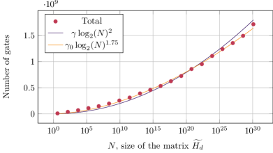
(a) Number of quantum gates versus simulated matrix size. The values of the constants $\gamma=250\,000$ and $\gamma_{0}=2\,000\,000$ have been chosen arbitrarily to fit the experimental data.

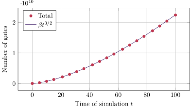
(b) Number of quantum gates versus physical time. The value of $\beta=39\,000\,000$ has been chosen arbitrarily to fit the experimental data.

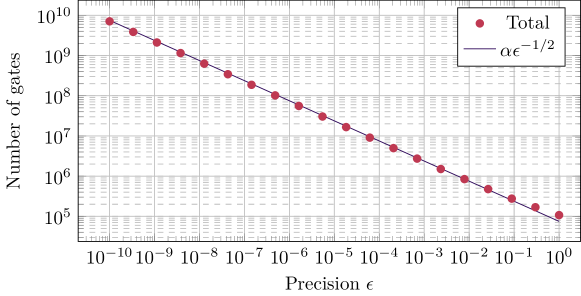
(c) Number of quantum gates versus targeted solution precision. The value of $\alpha=130\,000$ has been chosen arbitrarily to fit the experimental data.

Figure 1: Number of quantum gates needed to simulate the Hamiltonian described in appendix B using the oracles implemented following appendix C. Graphs generated with a Trotter-Suzuki product-formula order $k=1$, $32$ discretisation points (i.e. $n=6$ qubits) for fig. 1(b) and fig. 1(c), a physical time $t=1$ for fig. 1(a) and fig. 1(c) and a precision $\epsilon=10^{-5}$ for fig. 1(a) and fig. 1(b).

IV.2 Wave equation solver

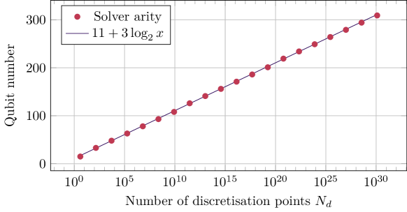
Figure 2: Plot of the number of logical qubits needed to run the wave equation solver for a time $t=1$, a precision $\epsilon=10^{-5}$ and a Trotter-Suzuki product-formula of order $k=1$. The constants values $11$ and $3$ have been chosen arbitrarily to fit the experimental data. The number of physical qubits needed will depend on their error rate as noted in Fowler et al. (2012). Multiplying the number of logical qubits by $3$ to $4$ orders of magnitude might be a good estimate of the actual number of physical qubits required.

The first characteristic of the wave equation solver that needs to be checked is its validity: is the quantum wave equation solver capable of solving accurately the wave equation as described in eq. 1 and eq. 2?

To check the validity of the solver, we used qat simulators and Atos QLM to simulate the quantum program generated to solve the wave equation with different values for the number of discretisation points $N_{d}$, for the physical time $t$ and for the precision $\epsilon$. fig. 3 shows the classical solution versus the quantum solution and the absolute error between the two solutions for $N_{d}=32$, $t=0.4$ and $\epsilon=10^{-3}$. The solution obtained by the quantum solver is nearly exactly the same as the classical solution obtained with finite differences. The error between the two solutions is of the order of $10^{-7}$, which is $4$ orders of magnitudes smaller than the error we asked for.

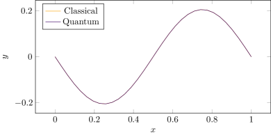
(a) Quantum versus classical solution. Solutions are not visually distinguishable on the graph, see the associated absolute error.

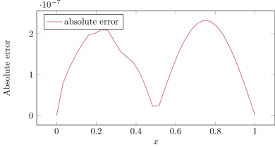
(b) Absolute error between the solution obtained by a classical finite-difference solver and the solution computed with the quantum solver.

Figure 3: Comparison of the classical solver and the quantum solver. Both solvers solved the $1$-D wave equation with $N_{d}=32$ discretisation points and a physical time of $t=0.4$. The classical solver uses finite-differences with a very small time-step in order to avoid as much as possible errors due to time-discretisation. The quantum solver was instructed to solve the wave equation with a precision of at least $\epsilon=10^{-3}$, used a Trotter-Suzuki order of $k=1$. The solutions of the two solvers are too close to be able to notice a difference (they overlap on the graph), that is why a second graph plotting the absolute error between the two solvers is included.

Once the validity of our solver has been checked on multiple test cases, the next interesting property we would like to verify is the asymptotic cost: does the implemented simulator seem to agree with the theoretical asymptotic complexities derived from Costa et al. (2019) and Berry et al. (2007)?

In our specific case, the Hamiltonian $H$ to simulate can be decomposed in two $1$-sparse Hermitian matrices, both of them having a spectral norm of $1$. The exact decomposition can be found in section B.3. We chose to let the product-formula order be equal to $k=1$ and reuse the asymptotic complexity found in eq. 15 by changing the time of simulation $t$ by the time $f(t)$:

$$\mathcal{O}\left(5^{2k}n^{2}f(t){\left(\frac{f(t)}{\epsilon}\right)}^{\frac{1}{2k}}\right).$$ (17)

Following the study performed in Costa et al. (2019),

$$f(t)=\frac{t}{\delta x}=t\left(N_{d}-1\right)$$ (18)

where $\delta x$ is the distance between two discretisation points. Moreover, it is possible to prove (see section B.3) that

$$n=\left\lceil\log_{2}(2N_{d}-1)\right\rceil$$ (19)

Replacing $f(t)$ and $n$ in eq. 10 and eq. 11 gives us a gate complexity of

$$\mathcal{O}\left(5^{k}\log_{2}\left(N_{d}\right)^{2}\right)$$ (20)

to construct a circuit simulating $e^{-iHt/r}$ and a number of repetitions

$$r\in\mathcal{O}\left(5^{k}tN_{d}{\left(\frac{tN_{d}}{\epsilon}\right)}^{\frac{1}{2k}}\right).$$ (21)

Merging the two expression results in a gate complexity of

$$\mathcal{O}\left(5^{2k}tN_{d}{\log_{2}(N_{d})}^{2}{\left(\frac{tN_{d}}{\epsilon}\right)}^{\frac{1}{2k}}\right).$$ (22)

Choosing the Totter-Suzuki formula order $k=1$ gives us a final complexity of

$$\mathcal{O}\left(N_{d}^{3/2}{\log_{2}(N_{d})}^{2}\frac{t^{3/2}}{\sqrt{\epsilon}}\right)$$ (23)

to solve the wave equation presented in eq. 1. This theoretical result is verified experimentally in fig. 4(a).

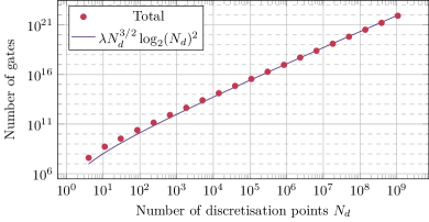
(a) Number of quantum gates needed to solve the wave equation described in eq. 1 versus discretisation size. The value of $\lambda=300\,000$ has been chosen arbitrarily to fit the experimental data.

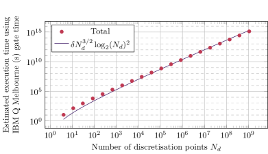
(b) Estimated execution time of the wave equation solver on IBM Q Melbourne hardware. Individual gate times have been extracted from mel (2019a) and mel (2019b). GF pulse time has been approximated via arithmetic mean to $347$ns, GD pulse time is $100$ns and buffer time is $20$ns. The value of $\delta=0.06$ has been chosen arbitrarily to fit the experimental data.

Figure 4: Graphs generated with a Trotter-Suzuki product-formula order $k=1$, a physical time $t=1$ and a precision $\epsilon=10^{-5}$.

V Discussion

In this work, we focus on the practical cost of implementing a $1$-dimensional quantum wave equation solver on a quantum computer. We show that a quantum computer is able to solve partial differential equations by constructing and simulating the quantum circuits described. We also study the scaling of the solver with respect to several parameters of interest and show that the theoretical asymptotic bounds are mostly verified.

In future works, one can study the possibilities of circuit optimisation. It would also be interesting to implement Neumann boundary conditions instead of Dirichlet ones. A practical implementation including a non-constant propagation speed $c$ has also been realised during the writing of this paper. The results were encouraging but were not judged mature enought to include them in the paper. Finally, future works might want to extend the wave equation solver to $2$ dimensions or more.

Supplementary material

The implementation of the quantum wave equation solver is available at https://gitlab.com/cerfacs/qaths. The qprof tool is available at https://gitlab.com/qcomputing/qprof/qprof.

Appendix A Product-formula implementation details

A.1 Hamiltonian simulation

Hamiltonian simulation is the problem of constructing a quantum circuit that will evolve a quantum state according to a Hamiltonian matrix, following the Schrödinger equation. In other words, Hamiltonian simulation algorithms generate a quantum circuit performing the unitary transformation $U$ such that $||U-e^{-iHt}||<\epsilon$, $H$ being a given Hamiltonian matrix, $t$ a time of evolution and $\epsilon$ a precision with respect to $||\cdot{}||$, the spectral norm.

Several quantum algorithms have been developed in the last few years to solve the problem of $s$-sparse Hamiltonian simulation Low and Chuang (2017b, 2016, a); Low (2018); Berry and Childs (2012); Berry et al. (2015a, 2007); Berry et al. (2015b); Kieferova et al. (2018); Shmoys et al. (2014); Childs and Wiebe (2012); Childs and Kothari (2011). Among these algorithms we decided to implement the product-formula approach Berry et al. (2007); Ahokas (2004), for the reasons presented in section III.1.

The product formula algorithm has three main steps: decompose, simulate, recompose. It works by first decomposing the $s$-sparse Hamiltonian matrix $H$ that should be simulated as a sum of Hermitian matrices $H_{j}$ that are considered easy to simulate

$$H=\sum_{j=0}^{m-1}H_{j}.$$ (24)

The second step is then to simulate each $H_{j}$ separately, i.e. to create quantum circuits implementing $e^{-iH_{j}t}$ for all the $H_{j}$ in the decomposition in eq. 24. The last step uses the simulations computed in step two to approximate $e^{-iHt}$.

The very first questions that should be answered before starting any implementation of the product-formula algorithm are “What is an easy to simulate matrix?” and “What kind of Hermitian matrices are easy to simulate?”.

A.2 Easy to simulate matrices

One of the most desirable properties for an “easy to simulate” matrix is the possibility to simulate it exactly, i.e. to construct a quantum circuit that will perfectly implement $e^{-iHt}$. This property becomes a requirement when one wants rigorous bounds on the error of the final simulation. Another enviable property of these matrices is that they can be simulated with a low gate number and only a few calls to the matrix oracle.

Definition 3 (Easy to simulate matrix).

A Hermitian matrix $H$ can be qualified as “easy to simulate” if there exist an algorithm that takes as input a time $t$ and the matrix $H$ and outputs a quantum circuit ${C(H)}_{t}$ such that

1. The quantum circuit ${C(H)}_{t}$ implements exactly the unitary transformation $e^{-iHt}$, i.e.

   $$\left|\left|e^{-iHt}-{C(H)}_{t}\right|\right|=0.$$

2. The algorithm only needs $\mathcal{O}\left(1\right)$ calls to the oracle of $H$ and $\mathcal{O}\left(\log N\right)$ additional gates, $N$ being the dimension of the matrix $H$.

With this definition of an “easy to simulate” matrix, we can now search for matrices or group of matrices that satisfy this definition.

A.2.1 Multiples of the identity

The first and easiest matrices that fulfil the easy to simulate matrix requirements are the multiples of the identity matrix $\left\{\alpha I,\,\alpha\in\mathbb{R}\right\}$ with $I$ the identity matrix. The quantum circuit to simulate this class of matrices can be found in Vazquez (2018).

A.2.2 $1$-sparse Hermitian matrices

A larger class of matrices that can be efficiently and exactly simulated are the $1$-sparse, integer weighted, Hermitian matrices. Quantum circuits simulating exactly $1$-sparse matrices with integer weights can be found in Ahokas (2004).

Note 3.

Procedures simulating $1$-sparse matrices with real (non-integers) weights are also described in the paper, but these matrices do not fall in the “easy to simulate” category because the procedures explained are exact only if all the matrix weights can be represented exactly with a fixed-point representation, which is not always verified.

Note 4.

Multiples of identity matrices presented in section A.2.1 are a special case of $1$-sparse matrices. The two classes have been separated because more efficient quantum circuits exists for $\alpha I$ matrices.

A.3 Decomposition of $H$

Once the set of “easy to simulate” matrices has been established, the next step of the algorithm is to decompose the $s$-sparse matrix $H$ as a sum of matrices in this set.

There are two possible ways of performing this decomposition, each one with its advantages and drawbacks: applying a procedure computing the decomposition automatically, or decompose the matrix $H$ beforehand and provide the decomposition to the algorithm.

The first solution, which is to automatically construct the oracles of the $H_{j}$ matrices from the oracle of the $H$ matrix has been studied in Ahokas (2004) and Childs and Kothari (2011). Thanks to this automatic decomposition procedure, we only need to implement one oracle. This simplicity comes at the cost of a higher gate count: each call to the automatically constructed oracles of the matrices $H_{j}$ will require several calls to the oracle of $H$ along with additional gates.

On the other hand, the second solution offers more control at the cost of less abstraction and more work. The decomposition of $H$ is not automatically computed and should be performed beforehand. Once the matrix $H$ has been decomposed as in eq. 9, the oracles for the matrices $H_{j}$ should be implemented. This means that we should now implement $m$ oracles instead of only $1$ for the first solution. The main advantage of this method over the one using automatic-decomposition is that it gives us more control, a control that can be used to optimize even more the decomposition of eq. 24 (less $H_{j}$ in the decomposition, $H_{j}$ matrices that can be simulated more efficiently, …).

All the advantages and drawbacks weighted, we chose to implement the second option for several reasons. First, the implementation of the automatic decomposition procedure adds a non-negligible implementation complexity to the whole Hamiltonian simulation procedure. Moreover, the automatic decomposition procedure can be implemented afterwards and plugged effortlessly to the non-automatic implementation. Finally, our use-case only required to simulate a $2$-sparse Hamiltonian that can be decomposed as the sum of two $1$-sparse, easy to simulate, Hermitian matrices, which makes the manual decomposition step manageable.

A.4 Simulation of the $H_{j}$

Once the matrix $H$ has been decomposed following eq. 24 with each $H_{j}$ being an “easy to simulate” matrix, the simulation of $H_{j}$ becomes a straightforward application of the procedures described in section A.2.

After this step, we have access to quantum circuits implementing $e^{-iH_{j}t}$ for $j\in\left[0,m-1\right]$ and $t\in\mathbb{R}$.

A.5 Re-composition of the $e^{-iH_{j}t}$

The ultimate step of the algorithm is to approximate the desired evolution $e^{-iHt}$ with the evolutions $e^{-iH_{j}t}$. In the special case of mutually commuting $H_{j}$, this step is trivial as it boils down to use the properties of the exponential function on matrices and write $e^{iHt}=e^{i\sum_{j}H_{j}t}=\prod_{j}e^{iH_{j}t}$. But in the more realistic case where the matrices $H_{j}$ do not commute, a more sophisticated method should be used to approximate the evolution $e^{-iHt}$. To this end, we used the first-order Lie-Trotter-Suzuki product formula defined in Definition definition 4.

Definition 4 (Lie-Trotter-Suzuki product formula Suzuki (1990, 1986); Childs et al. (2018)).

The Lie-Trotter-Suzuki product formula approximates

$$\exp\left(\lambda\sum_{j=0}^{m-1}\alpha_{j}H_{j}\right)$$ (25)

with

$$S_{2}(\lambda)=\prod_{j=0}^{m-1}e^{\alpha_{j}H_{j}\lambda/2}\prod_{j=m-1}^{0}e^{\alpha_{j}H_{j}\lambda/2}$$ (26)

and can be generalized recursively to higher-orders

$$S_{2k}\left(\lambda\right)={\left[S_{2k-2}\left(p_{k}\lambda\right)\right]}^{2}\times S_{2k-1}\left(\left(1-4p_{k}\right)\lambda\right){\left[S_{2k-2}\left(p_{k}\lambda\right)\right]}^{2}$$ (27)

with $p_{k}={\left(4-4^{1/(2k-1)}\right)}^{-1}$ for $k>1$. Using this formula, we have the approximation

$$e^{\lambda H}={\left[S_{2k}\left(\frac{\lambda}{n}\right)\right]}^{n}+\mathcal{O}\left(\frac{|\lambda|^{2k+1}}{n^{2k}}\right).$$ (28)

We used the Lie-Trotter-Suzuki product formula with $\lambda=-it$ to approximate the operator $e^{-iHt}$ up to an error of $\epsilon\in\mathcal{O}\left(\frac{t^{2k+1}}{n^{2k}}\right)$.

Appendix B Hermitian matrix construction and decomposition

One of the main challenge in implementing a quantum wave equation solver lies in the construction and implementation of the needed oracles. This appendix describes the first step of the implementation process: the construction and decomposition of the Hamiltonian matrix that will be simulated using the Hamiltonian simulation procedure introduced in appendix A.

This appendix follows the analysis performed in Costa et al. (2019) and adds details and observations that will be refereed to in appendix C when dealing with the actual oracle implementation.

B.1 Hamiltonian matrix description

In order to devise the Hamiltonian matrix that should be simulated to solve the wave equation, the first step is to discretise eq. 1 with respect to space. Such a discretisation can be seen as a graph $G_{\delta x}$ whose vertices are the discretisation points and with edges between nearest neighbour vertices. The graph $G_{\delta x}$ is depicted in fig. 5.

Figure 5: Graph $G_{\delta x}$ built from the discretisation of the $1$-dimensional line $[0,1]$ with $N_{d}$ discretisation points (i.e. $\delta x=\frac{1}{N_{d}-1}$).

The graph Laplacian of $G_{\delta x}$, defined as

$${L(G_{\delta x})}_{i,j}:=\begin{cases}\deg(v_{i})&\text{if }i=j\\ -1&\text{if }(i\neq j)\land(v_{i}\mbox{ adjacent to }v_{j})\\ 0&\text{otherwise}\\ \end{cases}$$ (29)

can then be used to approximate the differential operator $\frac{\partial^{2}}{\partial x^{2}}$. By using the discretisation approximation

$$\frac{\partial^{2}\phi}{\partial x^{2}}(i\delta x,t)\approx\frac{\phi_{i-1,t}-2\phi_{i,t}+\phi_{i+1,t}}{{\delta x}^{2}}$$ (30)

with $\phi_{i,t}=\phi(i\delta x,t)$, and approximating $\phi(x,t)$ with a vector $\phi={\left[\phi_{i,t}\right]}_{0\leqslant i<N_{d}}$, the matrix

$$A=-\frac{1}{{\delta x}^{2}}L(G_{\delta x})$$ (31)

approximates the second derivative of $\phi$ when $\delta x\to 0$ as

$${\left[A\phi\right]}_{i}=\frac{\phi((i-1)\delta x,t)-2\phi(i\delta x,t)+\phi((i+1)\delta x,t)}{{\delta x}^{2}}.$$ (32)

The approximation in eq. 31 is then used in eq. 1 to approximate the spatial derivative operator:

$$\frac{\partial^{2}}{\partial t^{2}}\phi=-\frac{1}{{\delta x}^{2}}L(G_{\delta x})\phi.$$ (33)

Based on this formula, Costa et al. (2019) shows that simulating

$$H=\begin{pmatrix}0&B\\ B^{\dagger}&0\\ \end{pmatrix}$$ (34)

with

$$BB^{\dagger}=L(G_{\delta x})$$ (35)

constructs a quantum circuit that will evolve a part of the quantum state it is applied on according to the discretised wave equation in eq. 33.

A matrix $B$ satisfying eq. 35 can be obtained directly from the graph $G_{\delta x}$ representing the discretisation. The algorithm to construct the matrix $B$ can be decomposed in three steps. First, the vertices (discretisation points) should be arbitrarily ordered by assigning them a unique index in $[0,N_{d}-1]$. Then, each edge of the graph is arbitrarily oriented and indexed with indices in $[0,N_{d}-2]$. Finally, $B$ is computed with the following definition

$$B_{ij}=\left\{\begin{array}[]{ll}1&\text{if edge }j\text{ is a self-loop of vertex }i\text{,}\\ 1&\text{if edge }j\text{ has vertex }i\text{ as source,}\\ -1&\text{if edge }j\text{ has vertex }i\text{ as sink,}\\ 0&\text{otherwise}\\ \end{array}\right..$$ (36)

Note that edges’ orientation and vertices/edges ordering is completely arbitrary. Changing either the edges orientation on one of the orderings will change the matrix $B$ but will not affect $BB^{\dagger}$ which should be equal to $L(G_{\delta x})$. This freedom in the ordering and orientation choices takes a crucial importance in the oracle implementation as it allows us to pick the ordering/orientation that will produce an easy-to-implement matrix $B$.

B.2 Dirichlet boundary conditions

Fixing boundary conditions is a requirement for most of the partial differential equations to admit a unique well-defined solution. There exist several boundary conditions such as Neumann, Dirichlet, Robin or Cauchy ones. For simplicity, we restricted ourselves to the study of eq. 1 with Dirichlet boundary condition of eq. 2.

In the case of Dirichlet boundary conditions on the $1$-dimensional line $[0,1]$, the two boundary nodes at $x=0$ and $x=1$ can be ignored as their value is always equal to $0$. Moreover, Costa et al. (2019) shows that the graph $G_{\delta x}^{D}$ representing the discretisation with Dirichlet boundary conditions of eq. 2 is simply $G_{\delta x}$ with self-loops on the two outer nodes (i.e. the ones indexed $1$ and $N_{d}-2$ as $0$ and $N_{d}-1$ are ignored). $G_{\delta x}^{D}$ is depicted in fig. 6. The algorithm to construct the matrix $B$ remain the same as explained in section B.1.

Figure 6: Graph $G_{\delta x}^{D}$ representing the discretisation of the 1-dimensional line $[0,1]$ with Dirichlet boundary conditions. The points and edges in grey are only drawn for illustration purpose and are ignored in the analysis because the boundary condition impose a value of $0$ on these vertices. Loops are added to $G_{\delta x}$ to encode the fact that this graph represents Dirichlet boundary conditions. Vertices (resp. edges) are ordered with indices within $[0,N_{c}-1]$ (resp. $[0,N_{c}+1]$). $N_{c}$ is the number of considered points and is equal to $N_{d}-2$ (the two extremal points are ignored).

B.3 Matrices construction

All the pieces are now in place to start building the matrix $B_{\text{d}}\in\mathbb{R}^{(N_{c}-1)\times N_{c}}$. Using the definition of the matrix $B$ written in eq. 36 and the graph $G_{\delta x}^{D}$ depicted in fig. 6 we end up with

$$B_{\text{d}}=\begin{pmatrix}1&1&0&\cdots&0\\ 0&-1&1&\ddots&\vdots\\ \vdots&\ddots&\ddots&\ddots&0\\ 0&\cdots&0&-1&1\\ \end{pmatrix}$$ (37)

We can easily check that $B_{\text{d}}B_{\text{d}}^{\dagger}$ is equal to the well-known discretisation matrix

$$B_{\text{d}}B_{\text{d}}^{\dagger}=\begin{pmatrix}2&-1&0&\cdots&0\\ -1&2&\ddots&\ddots&\vdots\\ 0&\ddots&\ddots&\ddots&0\\ \vdots&\ddots&\ddots&2&-1\\ 0&\cdots&0&-1&2\\ \end{pmatrix},$$ (38)

which validate the method of construction of $B_{\text{d}}$.

Computing $\widetilde{H_{\text{d}}}$, the Hamiltonian matrix that should be simulated to evolve the quantum state according to the wave equation in eq. 1 with Dirichlet boundary conditions, is now straightforward. Using eq. 34, we directly obtain

$$\widetilde{H_{d}}=\frac{1}{\delta x}\begin{pmatrix}0&\cdots&\cdots&0&1&1&0&\cdots&0\\ \vdots&&&\vdots&0&-1&1&\ddots&\vdots\\ \vdots&&&\vdots&\vdots&\ddots&\ddots&\ddots&0\\ 0&\cdots&\cdots&0&0&\cdots&0&-1&1\\ 1&0&\cdots&0&0&\cdots&\cdots&\cdots&0\\ 1&-1&\ddots&\vdots&\vdots&&&&\vdots\\ 0&1&\ddots&0&\vdots&&&&\vdots\\ \vdots&\ddots&\ddots&-1&\vdots&&&&\vdots\\ 0&\cdots&0&1&0&\cdots&\cdots&\cdots&0\\ \end{pmatrix}$$ (39)

As explained in appendix A, the Hamiltonian simulation algorithm implemented requires that the Hamiltonian to simulate is split as a sum of $1$-sparse Hermitian matrices. There are a lot of valid decompositions for the matrix $\widetilde{H_{d}}$ and we are free to choose the decomposition that will simplify the most the oracle implementation or reduce the gate complexity.

We made the choice to decompose $B_{\text{d}}$ as two $1$-sparse matrices and then reflect this decomposition on $\widetilde{H_{d}}$. Let $B_{1}$ and $B_{-1}$ defined as

$$B_{1}=\begin{pmatrix}0&1&0&\cdots&0\\ \vdots&\ddots&1&\ddots&\vdots\\ \vdots&&\ddots&\ddots&0\\ 0&\cdots&\cdots&0&1\\ \end{pmatrix}$$ (40)

$$B_{-1}=\begin{pmatrix}1&0&\cdots&\cdots&0\\ 0&-1&\ddots&&\vdots\\ \vdots&\ddots&\ddots&\ddots&\vdots\\ 0&\cdots&0&-1&0\\ \end{pmatrix}$$ (41)

we have $B_{\text{d}}=B_{1}+B_{-1}$. Let also

$$\widetilde{H_{1}}=\frac{1}{\delta x}\begin{pmatrix}0&B_{1}\\ {B_{1}}^{\dagger}&0\\ \end{pmatrix},\quad\widetilde{H_{-1}}=\frac{1}{\delta x}\begin{pmatrix}0&B_{-1}\\ {B_{-1}}^{\dagger}&0\\ \end{pmatrix},$$ (42)

it is easy to see that $\widetilde{H_{d}}=\widetilde{H_{1}}+\widetilde{H_{-1}}$ and that both $\widetilde{H_{1}}$ and $\widetilde{H_{-1}}$ are $1$-sparse Hermitian matrices.

For convenience, we also define

$$H_{1}=\begin{pmatrix}0&B_{1}\\ {B_{1}}^{\dagger}&0\\ \end{pmatrix},\quad H_{-1}=\begin{pmatrix}0&B_{-1}\\ {B_{-1}}^{\dagger}&0\\ \end{pmatrix},$$ (43)

and $H_{d}=H_{1}+H_{-1}$, the $\widetilde{H_{1}}$, $\widetilde{H_{-1}}$ and $\widetilde{H_{d}}$ matrices rescaled to contain only integer weights. These matrices have the interesting property that simulating $\widetilde{H_{d}}$ (resp. $\widetilde{H_{1}}$, $\widetilde{H_{-1}}$) for a time $t$ is equivalent to simulating $H_{d}$ (resp. $H_{1}$, $H_{-1}$) for a time $\frac{t}{\delta x}$. This property will be used in the following sections as it offers us the opportunity to simulate the integer-weighted matrices $H_{d}$, $H_{1}$ and $H_{-1}$ instead of the real-weighted ones $\widetilde{H_{d}}$, $\widetilde{H_{1}}$ and $\widetilde{H_{-1}}$.

Note also that a lower bound of the number of qubits needed to solve the wave equation for $N_{d}$ discretisation points can be computed from the dimensions of $H_{d}$. As the non-empty upper-left block of matrix $H_{d}$ is of dimension $\left(2N_{d}-1\right)\times\left(2N_{d}-1\right)$, we need at least

$$\left\lceil\log_{2}(2N_{d}-1)\right\rceil$$ (44)

qubits to simulate it. This estimation does not take into account ancilla qubits that may be needed to implement the oracles.

Appendix C Oracle construction

Oracles can be seen as the interface between a quantum procedure and real-world data. Their purpose is to encode classical data such that a quantum algorithm can process it efficiently.

C.1 Oracle interface

In order to work as a bridge between the classical and the quantum worlds and to be used by the quantum algorithm, a clear interface for the oracle should be established.

We chose to use the interface described in (Ahokas, 2004, Eq. 4.4) with slight modifications improving the arity of the oracle for our specific case of $1$-sparse matrices.

More precisely, our oracles $O$ implement the following interface

$$O\left|x_{0}\right\rangle_{x}\left|0\right\rangle_{m}\left|0\right\rangle_{v}\left|0\right\rangle_{s}=\left|x_{0}\right\rangle_{x}\left|m(x_{0})\right\rangle_{m}\left|v(x_{0})\right\rangle_{v}\left|s(x_{0})\right\rangle_{s}$$ (45)

with $\left|x_{0}\right\rangle_{x}$ encoding a row index as a unsigned integer, $m(x)$ the function that returns the column index of the only non-zero element in row $x$, $v(x)=|w(x)|$ the absolute value of the weight $w(x)$ of the first (and only) non-zero element in row $x$ and

$$s(x)=\left\{\begin{split}0&\text{ if }w(x)\geqslant 0\\ 1&\text{ else }\end{split}\right.$$ (46)

the sign of the first non-zero entry in row $x$.

Note that the quantum register are labeled with their respective usage: $x$ for the index of of the row considered, $m$ for the index of the column considered, $v$ for the value of the element at $(\mathrm{row},\mathrm{index})$ and $s$ for the sign of the element at $(\mathrm{row},\mathrm{index})$. A fifth label “$a$” is used along the paper to label a register used as an ancilla.

The interface of the oracle $O$ can also be obtained with 3 separate oracles that will each take care of computing one output:

$$M\left|x_{0}\right\rangle_{x}\left|0\right\rangle_{m}=\left|x_{0}\right\rangle_{x}\left|m(x)\right\rangle_{m}$$ (47)

$$V\left|x_{0}\right\rangle_{x}\left|0\right\rangle_{v}=\left|x_{0}\right\rangle_{x}\left|v(x)\right\rangle_{v}$$ (48)

$$S\left|x_{0}\right\rangle_{x}\left|0\right\rangle_{s}=\left|x_{0}\right\rangle_{x}\left|s(x)\right\rangle_{s}$$ (49)

C.2 Optimisation of $M$ and $S$

Claim 1.

The simulation algorithms provided by Ahokas (2004) have the interesting property that if the oracle $V$ encodes a weight of zero for some inputs (i.e. $v(x)=0$ for some $x$) then the outputs of oracles $M$ and $S$ are ignored for those inputs.

Proof.

The circuit simulating a $1$-sparse $m$-bit-integer weighted Hamiltonian $H$ depicted in fig. 7 is taken from Ahokas (2004).

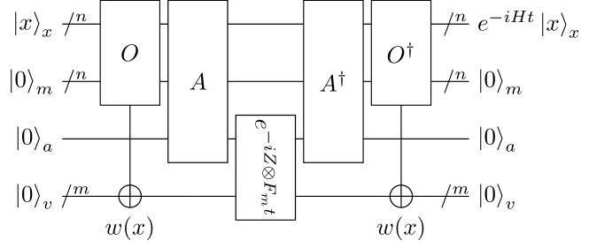
Figure 7: Quantum circuit re-created from (Ahokas, 2004, p. 71) that simulates a 1-sparse integer-weighted Hamiltonian for a given time $t$. $O$ is the implementation of the oracle, $A$ is a quantum circuit defined in (Ahokas, 2004, p. 70). $F_{m}$ is defined as the diagonal matrix with diagonal entries increasing from $0$ to $2^{m}-1$ (see eq. 51).

In our special case of $1$-bit weights (i.e. $m=1$), the third quantum gate $e^{-iZ\otimes F_{m}t}$ can be written as

$$\begin{split}e^{-iZ\otimes F_{m}t}&=e^{-iZ\otimes F_{1}t}\\ &=\exp\left[-i\begin{pmatrix}F_{1}&0\\ 0&-F_{1}\\ \end{pmatrix}t\right]\\ &=\begin{pmatrix}e^{-iF_{1}t}&0\\ 0&e^{iF_{1}t}\\ \end{pmatrix}\\ &=\begin{pmatrix}1&0&0&0\\ 0&e^{-it}&0&0\\ 0&0&1&0\\ 0&0&0&e^{-it}\\ \end{pmatrix}.\end{split}$$ (50)

where

$$F_{m}=\begin{pmatrix}0&0&\cdots&\cdots&\cdots&\cdots&0\\ 0&1&\ddots&&&&\vdots\\ \vdots&\ddots&2&\ddots&&&\vdots\\ \vdots&&\ddots&3&\ddots&&\vdots\\ \vdots&&&\ddots&4&\ddots&\vdots\\ \vdots&&&&\ddots&\ddots&0\\ 0&\cdots&\cdots&\cdots&\cdots&0&2^{m}-1\\ \end{pmatrix}.$$ (51)

It follows from the matrix notation that if the second qubit $e^{-iZ\otimes F_{1}t}$ is applied on is in the state $\left|0\right\rangle$, the gate $e^{-iZ\otimes F_{1}t}$ is the identity transformation, i.e. the unitary operation $e^{-iZ\otimes F_{1}t}$ sends $\left|00\right\rangle$ (resp. $\left|10\right\rangle$) to $\left|00\right\rangle$ (resp. $\left|10\right\rangle$). This means that if the oracle $O$ does not set the last qubit to $\left|1\right\rangle$ (i.e. the oracle encodes a weight of $0$ for the $x$^th row of $H$), the quantum circuit depicted in fig. 7 can be simplified up to an identity transformation as the effects of $O$ (resp. $A$) are reverted by $O^{\dagger}$ (resp. $A^{\dagger}$).

Rephrasing, if the $x$^th row of matrix $H$ has no non-zero entries, the effects of the oracle $O$ is ignored, which implies that the effects of the oracles $M$ and $S$ that compose $O$ are also ignored. ∎

Using the result of Claim 1, we are free to implement any transformation that best suits us for the set of inputs $\left|x\right\rangle$ such that the $x$^th row of the considered Hermitian matrix ($H_{1}$ or $H_{-1}$) has no non-zero elements as long as the oracle $V$ implements the right transformation.

To illustrate clearly the implemented transformations we chose to encode with $M$ and $S$, the next sections will re-write the matrices $H_{1}$ and $H_{-1}$ according to eq. 43 but with one $\mathbf{0}$ or $\mathbf{-0}$ in each empty row. A $\mathbf{0}$ entry at position $(i,j)$ in the matrix means that the row $i$ was empty, the oracle $M$ will map $\left|i\right\rangle_{x}$ to $\left|j\right\rangle_{m}$ and the oracle $S$ will encode a positive sign, i.e. $\left|0\right\rangle_{s}$. The same reasoning applies for $\mathbf{-0}$ entries, except that the encoded sign is now negative, i.e. $\left|1\right\rangle_{s}$.

The following sections will explain step by step the construction of each of the three oracles $M$, $V$ and $S$, both for the matrix $H_{1}$ ($M_{1}$, $V_{1}$ and $S_{1}$) and the matrix $H_{-1}$ ($M_{-1}$, $V_{-1}$ and $S_{-1}$).

C.3 About arithmetic and logic quantum gates

Implementing the oracles $M$, $V$ and $S$ for the matrices $H_{1}$ and $H_{-1}$ requires several arithmetic and logic quantum gates such as or, add or compare.

All these gates have been implemented prior to the oracle implementation and the implementation steps are detailed in this section.

C.3.1 The or gate

The or gate is easily implemented using only X and CCX (or Toffoli) gates. The implementation used is depicted in fig. 8 and uses the famous Boole algebra formula linking not, or and and: $x\vee y=\neg(\neg x\wedge\neg y)$.

=

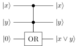
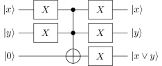
Figure 8: Implementation of the or gate.

C.3.2 The add and sub gates

Most of the research papers presenting an implementation of the add or sub gates only consider the case where the two numbers to add or subtract are stored in quantum registers.

In our case, the oracles implementation requires an adder and subtractor that can add or subtract to a quantum register a quantity known when the quantum circuit is generated, i.e. not necessarily encoded on a quantum state.

Claim 2.

Implementing a subtractor is trivial once an adder procedure is available.

Proof.

A subtractor can be implemented from a generic adder by using the identity

$$a-b=(a^{\prime}+b)^{\prime}$$ (52)

where ^′ denotes the bitwise complementation.

The circuit resulting of the application of this identity is depicted in fig. 9 and only requires one call to the adder and $2n$ additional gates, $n$ being the number of qubits used to represent one of the operands.

=

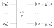
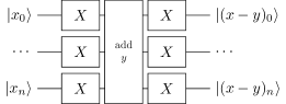
Figure 9: Implementation of the sub gate from an add gate. The $y$ value encoding is intentionally omitted. The subtractor will use the same encoding as the adder (i.e. either the $y$ value is encoded on a quantum register or it is encoded directly in the quantum circuit implementing the adder). Note that the $y$ value is not negated.

∎

Note 5.

Following Claim 2 we will restrict the study to implementing an adder. Implementing a subtractor is trivial and cheap in term of additional quantum gates used once an adder is available.

Definition 5.

Generation-time value A generation-time value is a value that is known by the programmer when generating the quantum circuit. Knowing a value at generation-time may allow to optimise even further the generated quantum circuit. The closest analog in classical programming would be C-like macros or recent C++ constexpr expressions.

The easiest solution to overcome the problem caused by the non-compatible input formats between our problem (with a generation-time value) and the existing adders (with two values encoded on quantum registers) is to encode the quantity known at generation-time into ancillary qubits and then use the regular adder algorithms to add to a quantum register the value encoded in a second quantum register. Even if this solution is trivial to implement, it has the huge downside of requiring $\mathcal{O}\left(\log_{2}b\right)$ additional ancillary qubits to temporarily store the generation-time value $b$.

Another answer to the problem would be to adapt a quantum adder originally devised to add two quantum registers to a quantum adder capable of adding a constant value to a quantum register. Several adders Thapliyal and Ranganathan (2017); Cuccaro et al. (2004); Draper (2000) have been studied to check if they can be modified to allow a generation-time input, i.e. if it possible to remove completely the quantum register storing the right-hand-side (or left-hand-side) of the addition.

The task of removing the quantum register storing one of the operands appears to be challenging for adders based on classical arithmetic like Cuccaro et al. (2004); Thapliyal and Ranganathan (2017) but trivial for Draper’s quantum adder introduced in Draper (2000).

Claim 3.

Draper’s quantum adder can be adapted into an efficient adder that takes as right-hand side input a unsigned “generation-time” integer value and add this value to a sufficiently large quantum register encoding another unsigned integer.

Proof.

The original Drapper’s adder as introduced in Draper (2000) is illustrated in fig. 10.

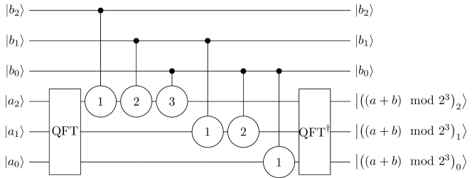
Figure 10: Original Draper’s adder example for $3$-qubit registers $\left|a\right\rangle$ and $\left|b\right\rangle$. The round gates between the two applications of the Quantum Fourier Transform (QFT gates) are controlled phase gates and are defined in Draper (2000). Note that the adder wraps on overflow, meaning that if an overflow happens, the result will be $(a+b)\mod 2^{3}$.

The only quantum gates using the quantum register $\left|b\right\rangle$ are the controlled-phase gates. Moreover, they only use the qubits of the right-hand-side register $\left|b\right\rangle$ as controls.

In the case of a constant value of $b$ known at generation time, we can replace each controlled-phase gate by either a phase gate if the corresponding bit of $b$ is $1$ or by an identity gate (or a “no-op” gate) if the bit of $b$ is $0$. Once this transformation has been performed, the quantum register $\left|b\right\rangle$ is no longer used and can be safely removed from the circuit. ∎

The final quantum add gate implementation is depicted in fig. 11, requires $\mathcal{O}\left(n^{2}\right)$ gates and has a depth of $\mathcal{O}\left(n\right)$. Following Barenco et al. (1996); Draper (2000); Cleve and Watrous (2000), the asymptotic gate count can be improved to $\mathcal{O}\left(n\log(n)\right)$ by removing the rotation with an angle below a given threshold that depend on hardware noise.

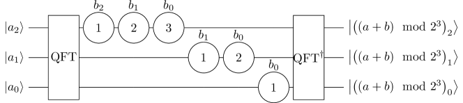
Figure 11: Modified Draper’s adder example for $3$-qubit register $\left|a\right\rangle$ and $3$-bit classical constant $b$. The round gates between the two applications of the Quantum Fourier Transform (QFT gates) are phase gates and are defined in Draper (2000). A label $b_{i}$ above a phase gate means that the phase gate should only be applied when the $i$^th bit of $b$ is set to $1$. Note that the adder wraps on overflow, meaning that if an overflow happens, the result will be $(a+b)\mod 2^{3}$.

C.3.3 The cmp gate

For the same reasons exposed in the adder implementation in section C.3.2, the cmp gate cannot be implemented using the arithmetic comparator presented in Cuccaro et al. (2004) because removing the right-hand side qubits seems to be a challenging task.

Instead, we use the idea from (Cuccaro et al., 2004, Section 4.3) that explain how to implement a comparator only by using a quantum adder. The comparison algorithm works by computing the high-bit of the expression $a-b$. If this high-bit is in the state $\left|1\right\rangle$ then $a<b$.

In order to compute the high-bit of $a-b$, several options are open. The two most promising options are described in the following paragraphs.

The first option is to use a subtractor acting on $n+1$ qubits and behaving nicely on underflows (i.e. underflows result in cycling to the highest-value), as illustrated in fig. 12. This approach requires $2$ calls to the subtractor and $1$ additional $2$-qubit quantum gate.

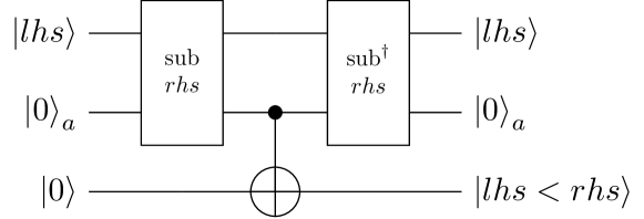
Figure 12: Computation of the high-bit of $lhs-rhs$ with a $(n+1)$-qubit subtractor. The second quantum register is an ancilla qubit that is appended to the quantum register storing $\left|\mathrm{lhs}\right\rangle$ in order to form a $(n+1)$-qubit register. The result is stored in a third quantum register as $\left|1\right\rangle$ if $lhs<rhs$, else $\left|0\right\rangle$.

Another solution would be to use eq. 52 to change the subtraction into an addition and then use a specialised procedure to compute the high-bit of the addition of two numbers $a$ and $b$ ($a$ being encoded on a quantum register and $b$ a constant). Computing the high-bit of an addition between a quantum register and a constant can be performed with the CARRY gate introduced in Häner et al. (2016). This approach requires $\mathcal{O}\left(n\right)$ Toffoli, CNOT and X gates.

Each of the described methods has its advantages and drawbacks.

For example, the first method crucially relies on a quantum subtractor, and will have the same properties as the subtractor used. In our specific case, we use the subtractor implemented with Drapper’s adder Draper (2000) as explained in section C.3.2, which in turn uses the quantum Fourier transform. The main disadvantage of using the QFT when looking at practical implementation on quantum hardware is that the QFT involves phase gates with exponentially small angles. These gates may be implemented correctly up to a given threshold, but very small rotation angles will inevitably not be as precise as normal rotation angles due to the hardware limitations in precision. This problem can be circumvented by using an approximate QFT algorithm Barenco et al. (1996); Cleve and Watrous (2000) that will cut all the rotation gates that have a rotation angle smaller than a given threshold from the generated circuit but the algorithm will not be exact anymore (small probability of incorrect result).

On the other hand, the CARRY gate involves only X, controlled-X and Toffoli gates. This restriction makes this implementation more robust than the first one to hardware approximations. Another difference is the connectivity needed by the approaches: the first method relies on a adder implemented with the quantum Fourier transform, which use an all-to-all connectity whereas the CARRY gate, once the qubits correctly ordered, only contains gates on adjacent qubits. As a side note, the exclusive use of logical gates X, controlled-X and Toffoli may allow us to simulate efficiently the CARRY gate on classical hardware as it only involves classical arithmetic.

As a last word, in the future, the QFT may be implemented directly into the hardware chips to make it more efficient because it is one of the most used quantum procedure (and so one of the best candidate for optimisation). Taking this possibility into account seems a little premature right now but may have a high impact on the efficiency and precision of the first solution presented.

After summarising all the drawbacks and advantages, we decided to use the arithmetic comparator for its linear number of gates, because it is based on arithmetic which does not involve exponentially small rotation angles and because the need to have $n-1$ dirty qubits to lend to the procedure is not an issue in our implementation.

C.3.4 The eq gate

The last gate the oracle implementation will need is an eq gate, testing the equality between an integer stored in a quantum register and a generation-time constant integer.

This gate has been implemented with a multi-controlled Tofolli gate and a few X gates before and after the control qubits of the Toffoli gates that should be equal to $\left|0\right\rangle$. The X gates are necessary because a raw Toffoli gate set its target qubit only when all its control are in the state $\left|1\right\rangle$, but we want each control qubit to be equal to a specific bit of the generation-time constant integer, which can be either $\left|0\right\rangle$ or $\left|1\right\rangle$.

An implementation example is available in fig. 13.

=

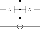
Figure 13: Example of eq gate implementation for the compile-time value $5$. X gates are applied to the second control qubit because the only bit set to $0$ in the big-endian binary representation of $5=101_{2}$ is at the second (middle) position.

Implementing a NOT gate controlled by $n$ qubits can be done with only one ancilla qubit or $n-2$ garbage qubits and requires $\mathcal{O}\left(n\right)$ X, controlled-X or Toffoli gates mul (2015).

C.4 Oracles for $H_{1}$

As noted in section C.2, the oracles $M_{1}$ and $S_{1}$ can be optimized by using the fact that they can encode anything for $\left|x\right\rangle_{x}$ when the $x$^th row of $H_{1}$ is empty.

We decided to use this optimization opportunity to add regularity to the description of the $H_{1}$ matrix. The implemented matrix $H_{1}$, denoted as $H_{1}^{\text{impl}}$, is described in eq. 53.

Note 6.

All indices start at $0$. The first row of a matrix has the index $0$, the second row the index $1$ and so on. This convention is used to match Python’s indexing that starts at $0$.

$$\begin{split}H_{1}^{\text{impl}}=\begin{array}[]{r}{\begin{array}[]{rrr}\overbrace{\hphantom{\begin{matrix}\vdots&0&\cdots&0\\ \vdots&-1&\ddots&\vdots\\ \vdots&1&\ddots&0\\ \vdots&\ddots&\ddots&-1\\ 0&\cdots&\cdots&\cdots\\ \end{matrix}}}^{N_{c}}&\overbrace{\hphantom{\begin{matrix}1&1&0&\cdots&0\\ 0&-1&1&\ddots&\vdots\\ \vdots&\ddots&\ddots&\ddots&\vdots\\ \cdots&\cdots&\cdots&\cdots&\vdots\\ \end{matrix}}}^{N_{c}+1}&{\overbrace{\hphantom{\begin{matrix}0&\cdots&\cdots&\cdots&\cdots&0\\ \vdots&&&&&\vdots\\ \vdots&&&&&\vdots\\ \vdots&&&&&\vdots\\ \end{matrix}}}^{2^{q}-\left(2N_{c}+1\right)}}\\ \end{array}}\\[0.0pt] \begin{array}[]{r}\rotatebox[origin={c}]{90.0}{$N_{c}$}\left\{\vphantom{\begin{matrix}1&1&0&\cdots&0\\ 0&-1&1&\ddots&\vdots\\ \vdots&\ddots&\ddots&\ddots&\vdots\\ \cdots&\cdots&\cdots&\cdots&\vdots\\ \end{matrix}}\right.\\[5.0pt] \rotatebox[origin={c}]{90.0}{$N_{c}+1$}\left\{\vphantom{\begin{matrix}\vdots&0&\cdots&0\\ \vdots&-1&\ddots&\vdots\\ \vdots&1&\ddots&0\\ \vdots&\ddots&\ddots&-1\\ 0&\cdots&\cdots&\cdots\\ \end{matrix}}\right.\\[5.0pt] \rotatebox[origin={c}]{90.0}{$2^{q}-\left(2N_{c}+1\right)$}\left\{\vphantom{\begin{matrix}0&\cdots&\cdots&\cdots\\ \vdots&&&\\ \vdots&&&\\ \vdots&&&\\ \vdots&&&\\ 0&\cdots&\cdots&\cdots\\ \end{matrix}}\right.\\ \end{array}\setcounter{MaxMatrixCols}{15}\begin{pmatrix}0&\cdots&\cdots&0&0&1&0&\cdots&0&0&\cdots&\cdots&\cdots&\cdots&0\\ \vdots&&&\vdots&\vdots&\ddots&\ddots&\ddots&\vdots&\vdots&&&&&\vdots\\ \vdots&&&\vdots&\vdots&&\ddots&\ddots&0&\vdots&&&&&\vdots\\ 0&\cdots&\cdots&0&0&\cdots&\cdots&0&1&0&&&&&\vdots\\ 0&\cdots&\cdots&0&0&\cdots&\cdots&\cdots&0&\mathbf{0}&&&&&\vdots\\ 1&\ddots&&\vdots&\vdots&&&&\vdots&0&&&&&\vdots\\ 0&\ddots&\ddots&\vdots&\vdots&&&&\vdots&\vdots&&&&&\vdots\\ \vdots&\ddots&\ddots&0&\vdots&&&&\vdots&\vdots&&&&&\vdots\\ 0&\cdots&0&1&0&\cdots&\cdots&\cdots&0&0&\cdots&\cdots&\cdots&\cdots&0\\ 0&\cdots&\cdots&0&\mathbf{0}&0&\cdots&\cdots&0&0&\cdots&\cdots&\cdots&\cdots&0\\ \vdots&&&&\ddots&\mathbf{0}&\ddots&&\vdots&\vdots&&&&&\vdots\\ \vdots&&&&&\ddots&\mathbf{\ddots{}}&\ddots&\vdots&\vdots&&&&&\vdots\\ \vdots&&&&&&\ddots&\mathbf{0}&0&0&&&&&\vdots\\ \vdots&&&&&&&\ddots&\mathbf{0}&0&\ddots&&&&\vdots\\ 0&\cdots&\cdots&\cdots&\cdots&\cdots&\cdots&\cdots&0&\mathbf{0}&0&0&\cdots&\cdots&0\\ \end{pmatrix}\end{array}\end{split}$$ (53)

According to the shape of the matrix in eq. 53, the oracle $M_{1}$ should implement the transformation

$$M_{1}|x\rangle_{x}|0\rangle_{m}\mapsto\begin{cases}|x\rangle_{x}\otimes|x+(N_{c}+1)\rangle_{m}&\text{if }x<(N_{c}+1)\\ |x\rangle_{x}\otimes|x-(N_{c}+1)\rangle_{m}&\text{else}\\ \end{cases}.$$ (54)

$M_{1}$ can be easily implemented with the quantum circuit depicted in fig. 14.

Figure 14: Implementation of the oracle $M_{1}$. The cmp gate compare the value of the control quantum register (interpreted as a unsigned integer) with the parameter given (written below the cmp). If the control register is strictly lower than the parameter, the gate set the qubit it is applied on to $\left|1\right\rangle$. The add (resp. sub) gate used in this quantum circuit add (resp. subtract) the value of its parameter to (resp. from) the quantum register it is applied on only if the control qubit is in the state $\left|1\right\rangle$.

The oracle $V$ cannot be simplified using the results from Claim 1. It should implement the transformation written in eq. 55.

$$V_{1}|x\rangle_{x}|0\rangle_{v}\mapsto\begin{cases}|x\rangle_{x}|1\rangle_{v}&\text{if }(x<2N_{c}+1)\land(x\neq N_{c})\\ |x\rangle_{x}|0\rangle_{v}&\text{else}\\ \end{cases}.$$ (55)

The implementation of the oracle $V_{1}$ is depicted in fig. 15. The first part, Set, sets the weight qubit to $1$ for all $\left|x\right\rangle_{x}$ such that $x<2N_{c}+1$. As this does not correspond to the correct expression of $V$, the second part Correct is here to set the weight register back to $\left|0\right\rangle_{v}$ when $x==N_{c}$.

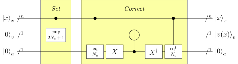
Figure 15: Implementation of the oracle $V_{1}$. The cmp gate compare the value of the control quantum register (interpreted as a unsigned integer) with the parameter given (written below the cmp). If the control register is strictly lower than the parameter, the gate set the qubit it is applied on to $\left|1\right\rangle$. The eq gate used in this quantum circuit sets its target qubit to $\left|1\right\rangle$ if the value of its parameter is equal to the value encoded on the quantum register controling the gate.

The last oracle left to implement in order to be able to simulate $H_{1}$ is $S_{1}$, the oracle encoding the signs of the non-zero entries of $H_{1}$. The convention used to encode the sign of an entry has been taken from Ahokas (2004) and is: a positive sign is encoded as $\left|0\right\rangle_{s}$, a negative sign is encoded as $\left|1\right\rangle_{s}$. As shown in eq. 53, $H_{1}$ only contains positive non-zero entries so the sign oracle $S_{1}$ should implement the simple transformation of eq. 56: the identity.

$$S_{1}|x\rangle_{x}|0\rangle_{s}\mapsto|x\rangle_{x}|0\rangle_{s}$$ (56)

C.5 Oracles for $H_{-1}$

The matrix $H_{-1}$ has less regularity than $H_{1}$, which will lead to a more complex implementation. The implemented matrix $H_{-1}$, denoted as $H_{-1}^{\text{impl}}$, is described in eq. 57.

$$\begin{split}H_{-1}^{\text{impl}}=\begin{array}[]{r}{\begin{array}[]{rrr}\overbrace{\hphantom{\begin{matrix}\vdots&0&\cdots&0\\ \vdots&-1&\ddots&\vdots\\ \vdots&1&\ddots&0\\ \vdots&\ddots&\ddots&-1\\ 0&\cdots&\cdots&\cdots\\ \end{matrix}}\hskip 4.30554pt}^{N_{c}}&\overbrace{\hphantom{\begin{matrix}0&-\mathbf{0}&\ddots&&\vdots\\ &\ddots&\ddots&\ddots&\vdots\\ &&\ddots&\ddots&0\\ &&&\ddots&-\mathbf{0}\\ &&&&\ddots\\ \cdots&\cdots&\cdots&\cdots&\cdots\\ \end{matrix}}\hskip 2.15277pt}^{N_{c}+1}&{\overbrace{\hphantom{\begin{matrix}0&\cdots&\cdots&\cdots&\cdots&0\\ \vdots&&&&&\vdots\\ \vdots&&&&&\vdots\\ 0&&&&&\vdots\\ \mathbf{0}&\ddots&&&&\vdots\\ 0&-\mathbf{0}&0&\cdots&\cdots&0\\ \end{matrix}\hskip 8.61108pt}}^{2^{q}-\left(2N_{c}+1\right)}}\\ \end{array}}\\[0.0pt] \begin{array}[]{r}\rotatebox[origin={c}]{90.0}{$N_{c}$}\left\{\vphantom{\begin{matrix}1&1&0&\cdots&0\\ 0&-1&1&\ddots&\vdots\\ \vdots&\ddots&\ddots&\ddots&\vdots\\ \cdots&\cdots&\cdots&\cdots&\vdots\\ \end{matrix}}\right.\\[5.0pt] \rotatebox[origin={c}]{90.0}{$N_{c}+1$}\left\{\vphantom{\begin{matrix}\vdots&0&\cdots&0\\ \vdots&-1&\ddots&\vdots\\ \vdots&1&\ddots&0\\ \vdots&\ddots&\ddots&-1\\ 0&\cdots&\cdots&\cdots\\ \end{matrix}}\right.\\[5.0pt] \rotatebox[origin={c}]{90.0}{$2^{q}-\left(2N_{c}+1\right)$}\left\{\vphantom{\begin{matrix}0&-\mathbf{0}&\ddots&&\vdots\\ &\ddots&\ddots&\ddots&\vdots\\ &&\ddots&\ddots&0\\ &&&\ddots&-\mathbf{0}\\ &&&&\ddots\\ \cdots&\cdots&\cdots&\cdots&\cdots\\ \end{matrix}}\right.\\ \end{array}\setcounter{MaxMatrixCols}{15}\begin{pmatrix}0&\cdots&\cdots&0&1&0&\cdots&\cdots&0&0&\cdots&\cdots&\cdots&\cdots&0\\ \vdots&&&\vdots&0&-1&\ddots&&\vdots&\vdots&&&&&\vdots\\ \vdots&&&\vdots&\vdots&\ddots&\ddots&\ddots&\vdots&\vdots&&&&&\vdots\\ 0&\cdots&\cdots&0&0&\cdots&0&-1&0&\vdots&&&&&\vdots\\ 1&0&\cdots&0&0&\cdots&\cdots&\cdots&0&\vdots&&&&&\vdots\\ 0&-1&\ddots&\vdots&\vdots&&&&\vdots&\vdots&&&&&\vdots\\ \vdots&\ddots&\ddots&0&\vdots&&&&\vdots&\vdots&&&&&\vdots\\ \vdots&&\ddots&-1&0&&&&\vdots&\vdots&&&&&\vdots\\ 0&\cdots&\cdots&0&-\mathbf{0}&\ddots&&&\vdots&0&\cdots&\cdots&\cdots&\cdots&0\\ 0&\cdots&\cdots&\cdots&0&-\mathbf{0}&\ddots&&\vdots&0&\cdots&\cdots&\cdots&\cdots&0\\ \vdots&&&&&\ddots&\ddots&\ddots&\vdots&\vdots&&&&&\vdots\\ \vdots&&&&&&\ddots&\ddots&0&\vdots&&&&&\vdots\\ \vdots&&&&&&&\ddots&-\mathbf{0}&0&&&&&\vdots\\ \vdots&&&&&&&&\ddots&-\mathbf{0}&\ddots&&&&\vdots\\ 0&\cdots&\cdots&\cdots&\cdots&\cdots&\cdots&\cdots&\cdots&0&-\mathbf{0}&0&\cdots&\cdots&0\\ \end{pmatrix}\end{array}\end{split}$$ (57)

Following the placement of the non-zero and the $\mathbf{0}$ or $-\mathbf{0}$ entries in the matrix $H_{-1}^{\text{impl}}$ of eq. 57, the oracle $M_{-1}$ should implement the transformation

$$M_{-1}|x\rangle_{x}|0\rangle_{m}\mapsto\begin{cases}|x\rangle_{x}|x+N_{c}\rangle_{m}&\text{if }x<N_{c}\\ |x\rangle_{x}|x-N_{c}\rangle_{m}&\text{else}\\ \end{cases}.$$ (58)

This transformation is quite similar to the one implemented by the oracle $M_{1}$ in eq. 54: $N_{c}+1$ from the transformation $M_{1}$ has been replaced by $N_{c}$ in the transformation $M_{-1}$. Thanks to this similarity, the implementation of $M_{-1}$ will be a nearly-exact copy of the implementation of $M_{1}$. The full implementation of the $M_{-1}$ oracle is depicted in fig. 16.

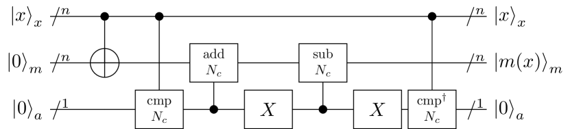
Figure 16: Implementation of the oracle $M_{-1}$. The cmp gate compare the value of the control quantum register (interpreted as a unsigned integer) with the parameter given (written below the cmp). If the control register is strictly lower than the parameter, the gate set the qubit it is applied on to $\left|1\right\rangle$. The add (resp. sub) gate used in this quantum circuit add (resp. subtract) the value of its parameter to (resp. from) the quantum register it is applied on only if the control qubit is in the state $\left|1\right\rangle$.

The weight oracle $V_{-1}$ is the simplest to implement for the matrix $H_{-1}$, even if it cannot take advantage of the optimisation discussed in Claim 1. The transformation that should be implemented by the oracle $V_{-1}$ is shown in eq. 59.

$$V_{-1}|x\rangle_{x}|0\rangle_{v}\mapsto\begin{cases}|x\rangle_{x}|1\rangle_{v}&\text{if }x<2N_{c}\\ |x\rangle_{x}|0\rangle_{v}&\text{else}\\ \end{cases}.$$ (59)

The implementation of the weight oracle $V_{-1}$ is illustrated in fig. 17.

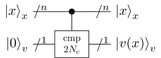
Figure 17: Implementation of the oracle $V_{-1}$. The cmp gate compare the value of the control quantum register (interpreted as a unsigned integer) with the parameter given (written below the cmp). If the control register is strictly lower than the parameter, the gate set the qubit it is applied on to $\left|1\right\rangle$.

The last oracle left to implement is $S_{-1}$, the sign oracle. Due to the sign irregularity in the matrix $H_{-1}^{\text{impl}}$, the implementation of $S_{-1}$ is more involved and requires several ancillary qubits. According to the shape of the matrix $H_{-1}^{\text{impl}}$, the sign oracle $S_{-1}$ should implement the transformation defined in eq. 60.

$$S_{-1}|x\rangle_{x}|0\rangle_{s}\mapsto\begin{cases}|x\rangle_{x}|0\rangle_{s}&\text{if }(x=0)\lor(x=N_{c})\\ |x\rangle_{x}|1\rangle_{s}&\text{else}\\ \end{cases}.$$ (60)

An implementation of the oracle $S_{-1}$ is illustrated in fig. 18.

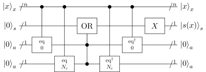
Figure 18: Implementation of the oracle $S_{-1}$. The eq gate used in this quantum circuit is presented in fig. 13 and test if the value encoded in its control qubits is equal to the compile-time value given. The OR gate flips the target qubits if and only if at least one of the two control qubits is in the state $\left|1\right\rangle$.

Appendix D Implementation of higher-order Laplacians

The results shown in this paper have all been generated using the second-order discretisation formula shown in eq. 30. Higher-order formulas are studied in (Costa et al., 2019, VI, VII and C).

Note 7.

As shown in (Costa et al., 2019, VII.B), higher-order discretisations with Neumann boundary conditions are not implementable using the algorithm described in appendix B.

In this appendix we replace the second-order formula given in eq. 30 and used all along the paper by the fourth-order formula given in (Costa et al., 2019, Eq. (46)) and re-written below

$$\frac{\partial^{2}\phi}{\partial x^{2}}(i\delta x,t)\approx\frac{1}{{\delta x}^{2}}\left(\frac{5}{2}\phi_{i,t}-\frac{4}{3}\left(\phi_{i-1,t}+\phi_{i+1,t}\right)+\frac{1}{12}\left(\phi_{i-2,t}+\phi_{i+2,t}\right)\right).$$ (61)

We are left to devise the matrix $B_{d}^{4}$ that satisfy $B_{d}^{4}{B_{d}^{4}}^{\dagger}=\Delta_{4}$ where $\Delta_{4}$ is the discretisation matrix arising from the fourth-order finite-differences approximation in eq. 61.

(Costa et al., 2019, Eq. (47) and VII.C) devised an analytic formula for $\hat{B}_{d}^{4}$, the $B_{d}^{4}$ matrix with periodic boundary conditions, using the matrix $\hat{S}$ representing the cyclic permutation $\{1,2,\dots,N\}$ with entries $\hat{S}_{i,j}=\delta_{i,(j+1\mod N)}$ as shown in eq. 62.

$$\hat{S}=\begin{pmatrix}0&0&\cdots&\cdots&\cdots&0&1\\ 1&0&&&&&0\\ 0&\ddots&\ddots&&&&\vdots\\ \vdots&\ddots&\ddots&\ddots&&&\vdots\\ \vdots&&\ddots&\ddots&\ddots&&\vdots\\ \vdots&&&\ddots&\ddots&\ddots&\vdots\\ 0&\cdots&\cdots&\cdots&0&1&0\\ \end{pmatrix}$$ (62)

With this definition of $\hat{S}$, the analytic formula for $\hat{B}_{d}^{4}$ is given in eq. 65, with $b$ and $c$ being solution of (Costa et al., 2019, Eqs. (53,54,55)). The exact values for $b$ and $c$ are:

$$b=\pm\frac{1}{2\sqrt{3}\sqrt{7\pm 4\sqrt{3}}}$$ (63)

$$c=\pm\sqrt{\frac{7\pm 4\sqrt{3}}{12}}$$ (64)

with the $\pm$ signs that can be chosen freely. Note that, $b=\pm\frac{1}{2\sqrt{3}\sqrt{7\pm 4\sqrt{3}}}$ and $c=\frac{1}{12b}$ are irrational because $\sqrt{3}\sqrt{7\pm 4\sqrt{3}}=\sqrt{3}\sqrt{2+\sqrt{3}}^{2}=\sqrt{3}\left(2+\sqrt{3}\right)=2\sqrt{3}+3$ is irrational.

eq. 66 shows the matrix shape with its entries.

$$\hat{B}_{d}^{4} =c\hat{S}-(b+c)*\mathbb{I}+b\hat{S}^{\dagger}$$ (65)

$$\approx\begin{pmatrix}b+c&b&0&\cdots&\cdots&\cdots&0&c\\ c&b+c&b&\ddots&&&&0\\ 0&c&\ddots&\ddots&\ddots&&&\vdots\\ \vdots&\ddots&\ddots&\ddots&\ddots&\ddots&&\vdots\\ \vdots&&\ddots&\ddots&\ddots&\ddots&\ddots&\vdots\\ \vdots&&&\ddots&\ddots&\ddots&b&0\\ 0&&&&\ddots&c&b+c&b\\ b&0&\cdots&\cdots&\cdots&0&c&b+c\\ \end{pmatrix}$$ (66)

Because periodicity has not been studied in the main use-case of this paper, we would like to also remove the need of periodic boundary conditions in this higher-order laplacian discretisation. This can be achieved by removing the upper-right entry of $\hat{S}$ by changing it from $1$ to $0$. The resulting matrix $S$ is shown in eq. 67.

$$S=\begin{pmatrix}0&0&\cdots&\cdots&\cdots&\cdots&0\\ 1&0&&&&&\vdots\\ 0&\ddots&\ddots&&&&\vdots\\ \vdots&\ddots&\ddots&\ddots&&&\vdots\\ \vdots&&\ddots&\ddots&\ddots&&\vdots\\ \vdots&&&\ddots&\ddots&\ddots&\vdots\\ 0&\cdots&\cdots&\cdots&0&1&0\\ \end{pmatrix}$$ (67)

Using the exact same formula we can devise $B_{d}^{4}$:

$$B_{d}^{4} =cS-(b+c)*\mathbb{I}+bS^{\dagger}$$ (68)

$$\approx\begin{pmatrix}b+c&b&0&\cdots&\cdots&\cdots&\cdots&0\\ c&b+c&b&\ddots&&&&\vdots\\ 0&c&\ddots&\ddots&\ddots&&&\vdots\\ \vdots&\ddots&\ddots&\ddots&\ddots&\ddots&&\vdots\\ \vdots&&\ddots&\ddots&\ddots&\ddots&\ddots&\vdots\\ \vdots&&&\ddots&\ddots&\ddots&b&0\\ \vdots&&&&\ddots&c&b+c&b\\ 0&\cdots&\cdots&\cdots&\cdots&0&c&b+c\\ \end{pmatrix}$$ (69)

Replacing $B_{d}^{4}$ in eq. 34 we obtain

$$\widetilde{H_{d}^{4}}=\frac{1}{\delta x}\begin{pmatrix}0&\cdots&\cdots&\cdots&0&b+c&b&0&\cdots&0\\ \vdots&&&&\vdots&c&b+c&b&\ddots&\vdots\\ \vdots&&&&\vdots&0&c&\ddots&\ddots&0\\ \vdots&&&&\vdots&\vdots&\ddots&\ddots&b+c&b\\ 0&\cdots&\cdots&\cdots&0&0&\cdots&0&c&b+c\\ b+c&c&0&\cdots&0&0&\cdots&\cdots&\cdots&0\\ b&b+c&\ddots&\ddots&\vdots&\vdots&&&&\vdots\\ 0&\ddots&\ddots&\ddots&0&\vdots&&&&\vdots\\ \vdots&\ddots&\ddots&b+c&c&\vdots&&&&\vdots\\ 0&\cdots&0&b&b+c&0&\cdots&\cdots&\cdots&0\\ \end{pmatrix}.$$ (70)

One of the main difference with the second-order approximation used all along this paper is that, with the fourth-order approximation, the entries of the matrix $\widetilde{H_{d}^{4}}$ are no longer multiples of a common number $\alpha\in\mathbb{R}$. This means that we cannot write down $\widetilde{H_{d}^{4}}$ as an integer weighted matrix multiplied by a real number, and so the trick used in section B.3 to simulate the integer weighted matrix $H_{d}$ for a time $\alpha t$ is no longer applicable.

Consequently, and independently of the decomposition we use for $\hat{H_{d}^{4}}$, at least one of the matrices in the decomposition of $\hat{H_{d}^{4}}$ will not be “easy to simulate” as defined in Definition definition 3.

Ultimately, the main consequence of this observation is that we will have to use a real-weighted hamiltonian simulation procedure. Such a procedure can be found in Ahokas (2004) but requires to approximate the real-weighted entries with a fixed-point representation that has at least 2 evident caveats:

1. It is impossible to encode the irrational numbers $b$ and $c$ exactly with a fixed-point representation. This means that we add another layer of approximation, even before the approximation caused by the use of a product-formula.

2. The hamiltonian simulation procedures used for real numbers requires more qubits. More precisely, the number of additional qubits required depends on the desired precision $\epsilon$ and grows as $\log_{2}\left(\frac{1}{\epsilon}\right)$.

Note 8.

Even if the $H_{d}^{4}$ matrix seems quite hard to simulate, it is still a $3$-sparse matrix. This means that it is still managable to hand-write the oracles. Moreover, having a small number of matrices in the decomposition helps in reducing the error introduced by product-formulas.

Appendix E Optimisation of the implementation

Once the correctness of the implementation validated, one of the most important remaining work is to try to optimise the implementation. The optimisation of a software is often performed as an iterative task.

The first step is to define a figure of merit, a quantity we want to minimise during the optimisation process. Among the most obvious figures of merit are the total number of gates, the number of CNOT gates or the total execution time of the quantum program. More complex quantities can also be considered, such as the execution time using error correction codes or the final state fidelity. In this paper we decided to take into account an estimation of the total execution time of the quantum program on an imaginary device that shares today’s chips characteristics.

The second step of the optimisation process consists in isolating the subroutines that contribute the most to the figure of merit. As an example, if the quantum program spend $90\%$ of the total execution time in one subroutine, this subroutine should be the first place to look for optimisations.

After the isolation of one or two subroutines, the actual optimisation can take place. The goal of this third step is to decrease the impact of the subroutines considered on the overall figure of merit without changing the final result of the implementation.

Finally, once the optimisation is performed, the optimisation process can be repeated by re-starting at the second step, until the program is considered sufficiently optimised.

One of the main difficulty we encountered when applying this optimisation process was to correctly isolate the most time-consumming subroutines. In classical computing, this step is usually performed with specialised tools such as gprof or a more advanced profiler, but no such tool exist for quantum programs. In order to fill this gap we developped qprof, a tool that analyses a quantum program and generates a report similar to the one generated by gprof. Using qprof and some of the various tools compatible with gprof, we plotted the call-graph shown in fig. 19(a).

From this call-graph, it is clear that the adder is the most costly subroutine and that it should be optimised. The adder internally uses the Quantum Fourier Transform (QFT), which takes more than $50\%$ of the total execution time. The issue is that the QFT implementation is already very concise and we do not expect to be able to optimise it enough to cut significantly its overall cost. This leads us to the conclusion that a new algorithm that do not require the QFT should be used to implement an adder. Such an algorithm can be found in Vedral et al. (1996).

Changing the implementation of the adder from Draper’s adder to the arithmetic-based adder from Vedral et al. (1996) improves drastically the total execution time of the quantum program and produce the call-graph in fig. 19(b).

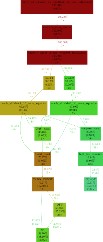
(a) Call graph of the quantum wave equation solver using Draper’s adder (QFT-based).

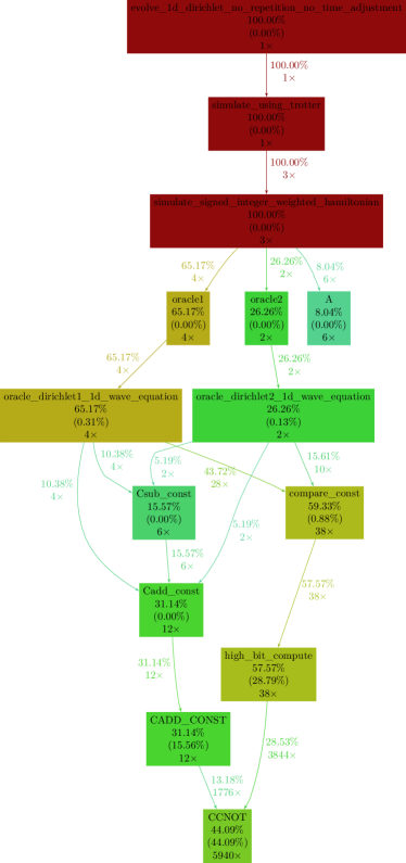
(b) Call graph of the quantum wave equation solver using an arithmetic-based adder.

Figure 19: All the gates or subroutines that account for less than $5\%$ of the total execution time are not displayed. Execution times for $u1$, $u2$, $u3$ and $cx$ gates have been averaged over all the data available for the quantum chip IBMQ Melbourne. Using the arithmetic-based adder, the overall execution time improved by a factor of $31$.

Appendix F Gate count analysis

F.1 Precise subroutines gate counts

table 1 summarise the gate count and ancilla qubit requirements for all the major subroutines used in the wave equation solver implementation. Using the entries of this table, it is possible to compute an estimation of the number of gates required to solve the wave equation.

As explained in appendix A, we need to simulate each of the $1$-sparse Hamiltonians in the decomposition. Aggregating the estimates in table 1 we obtain the costs in table 2 for the Hamiltonian simulation part. Note that the cost of the adder has been voluntarily omited from the computations in order to be able to compare the cost with different adder implementations. Let $a$ be the gate cost of the adder implementation chosen, the cost of simulating the Hamiltonian needed to solve the $1$-dimensional wave equation is: $82n-35+12a_{\mathtt{Toffoli}}$ Toffoli gates, $84n+21+9\left[0,n-1\right]+12a_{\mathtt{CNOT}}$ CNOT gates and $\mathcal{O}\left(n\right)+12a_{1-\mathtt{qubit}}$ $1$-qubit gates.

Choosing an adder implementation and simplifying the gate counts by omitting negligible terms we obtain the gate counts summarised in table 3. It is interesting to note that even if the arithmetic-based adder adds huge constants in the gate count, it does not change the asymptotic complexity whereas Draper’s adder changes the number of CNOT gates required from $\mathcal{O}\left(n\right)$ to $\mathcal{O}\left(n^{2}\right)$.

Gate	Toffoli count	CNOT count	$1$-qubit gate count	# ancillas	notes
or	1	0	5	0
QFT	0	$3\left(2n^{2}-2n+\lfloor\frac{n}{2}\rfloor\right)$	$2\left(n^{2}+n\right)$ $H$ $4\left(n^{2}-n\right)$ $T$ $\frac{n^{2}-n}{2}$ $R_{n}$	1 $\left|0\right\rangle$-init	$R_{n}$ gates might need to be decomposed Ross and Selinger (2014).
add_arith	$20n-10$	$22n$	$0$	$n-1$ $\left|0\right\rangle$-init	See Vedral et al. (1996).
add_qft	0	$6\left(2n^{2}-2n+\lfloor\frac{n}{2}\rfloor\right)$	$2\left(n^{2}+n\right)$ $H$ $4\left(n^{2}-n\right)$ $T$ $3\frac{n^{2}-n}{2}$ $R_{n}$	1 $\left|0\right\rangle$-init	See QFT note on $R_{n}$. fig. 11.
sub_qft	0	$6\left(2n^{2}-2n+\lfloor\frac{n}{2}\rfloor\right)$	$2\left(n^{2}+n\right)$ $H$ $4\left(n^{2}-n\right)$ $T$ $3\frac{n^{2}-n}{2}$ $R_{n}$ $2n$ $X$	1 $\left|0\right\rangle$-init	See QFT note on $R_{n}$. fig. 9.
CARRY	$2(n-1)$	$2+\left[0,n-1\right]$	$2n+\left[0,n-1\right]$ $X$	$n-1$ borrowed	See Häner et al. (2016).
$n$-contr. CNOT	$4n$	$0$	$0$	$n$ borrowed	See mul (2015).
eq	$4n$	$0$	$2\left[0,n\right]$ $X$	$n$ borrowed	fig. 13.
cmp	$2\left(n-1\right)$	$2+\left[0,n-1\right]$	$4n+\left[0,n-1\right]$ $X$	$n-1$ borrowed	See CARRY and section C.3.3.
A	$2n$	$4n$	$3n$ $H$ $3n$ $S$ $2n$ $T$ $2n$ $X$	0	See (Ahokas, 2004, Fig. 4.3.).
$e^{-iZ\otimes Z\otimes Ft}$	$8n$	$24n$	$36n$ $P_{h}$ $8$ $X$	0	Adapted from (Ahokas, 2004, Fig. 4.6)
$1$-sparse HS	$10n$	$28n$	$3n$ $H$ $3n$ $S$ $2n$ $T$ $2n+8$ $X$ $36n$ $P_{h}$	0	Oracle implementation cost not included. $2$ calls to the oracle are required. fig. 7.
$M_{1}$	$4\left(n-1\right)$	$5+2\left[0,n-1\right]$	$10n+2+\left[0,n-1\right]$ $X$	$1$ $\left|0\right\rangle$-init $n-1$ borrowed	add implementation cost not included. $2$ calls to add are required. fig. 14.
$V_{1}$	$2\left(n-1\right)$	$2+\left[0,n-1\right]$	$4n+\left[0,n-1\right]$ $X$	$n-1$ borrowed	fig. 15.
$S_{1}$	$0$	$0$	$0$	$0$	eq. 56.
$M_{-1}$	$4\left(n-1\right)$	$5+2\left[0,n-1\right]$	$10n+2+\left[0,n-1\right]$ $X$	$1$ $\left|0\right\rangle$-init $n-1$ borrowed	add implementation cost not included. $2$ calls to add are required. fig. 16.
$V_{-1}$	$2\left(n-1\right)$	$2+\left[0,n-1\right]$	$4n+\left[0,n-1\right]$ $X$	$n-1$ borrowed	fig. 17.
$S_{-1}$	$16n+1$	$0$	$5+8\left[0,n\right]$ $X$	$n$ borrowed	fig. 18.

Table 1: Precise gate count for the most important subroutines used in the quantum implementation of the wave equation solver. $n$ always reprensent the size of the input(s), except for the $n$-controlled CNOT where $n$ is the number of controls. When the number of gates depends on a generation-time value, the range of all the integer values possible is shown with square brackets. For example, $\left[0,n-1\right]$ means that, depending on the generation-time value provided, the number of gates will be an integer between $0$ and $n-1$ included. $\left|0\right\rangle$-init ancillas represent the standard ancilla-type: qubits that are given in the state $\left|0\right\rangle$ and should be returned in that exact same state. On the other side, borrowed ancillas can be given in any state and should be returned in the exact same state they were borrowed in.

Unitary	Toffoli count	CNOT count	$1$-qubit gate count	# ancillas	notes
$e^{-iH_{1}t}$	$22n-12$	$28n+7+3\left[0,n-1\right]$	$3n$ $H$ $3n$ $S$ $2n$ $T$ $36n$ $P_{h}$ $30n+10+2\left[0,n-1\right]$ $X$	$1$ $\left|0\right\rangle$-init $n-1$ borrowed	add implementation cost not included. $4$ calls to add are required.
$e^{-iH_{-1}t}$	$38n-11$	$28n+7+3\left[0,n-1\right]$	$3n$ $H$ $3n$ $S$ $2n$ $T$ $36n$ $P_{h}$ $30n+15+10\left[0,n\right]$ $X$	$1$ $\left|0\right\rangle$-init $n-1$ borrowed	add implementation cost not included. $4$ calls to add are required.
$e^{-iHt}$	$82n-35$	$84n+21+9\left[0,n-1\right]$	$9n$ $H$ $9n$ $S$ $6n$ $T$ $108n$ $P_{h}$ $90n+35+14\left[0,n\right]$ $X$	$1$ $\left|0\right\rangle$-init $n-1$ borrowed	add implementation cost not included. $12$ calls to add are required.

Table 2: Number of gates and ancillas needed to simulate the easy-to-simulate Hamiltonians $H_{1}$ and $H_{-1}$ that are part of the decomposition of $H$ as well as $e^{-iHt}$. It is important to realise that the gate counts for $e^{-iHt}$ are only valid up to a given $t$ or $\epsilon$ (once one is fixed, the value of the other can be computed). In order to make the gate count generic for any $t$ and $\epsilon$, the number of repetitions should be computed (see $n$ in eq. 28). Note that some of the $\left[0,n-1\right]$ ranges have been simplified to $\left[0,n\right]$ for conciseness.

Adder used	Toffoli count	CNOT count	$1$-qubit gate count	# ancillas
add_qft	$82n-35$	$144n^{2}-60n$	$24n^{2}+25n$ $H$ $9n$ $S$ $48n^{2}-42n$ $T$ $108n$ $P_{h}$ $18n^{2}-18n$ $R_{n}$ $114n+35+14\left[0,n\right]$ $X$	$2$ $\left|0\right\rangle$-init $n-1$ borrowed
add_arith	$222n-175$	$348n+21+9\left[0,n-1\right]$	$9n$ $H$ $9n$ $S$ $6n$ $T$ $108n$ $P_{h}$ $90n+35+14\left[0,n\right]$ $X$	$n$ $\left|0\right\rangle$-init $n-1$ borrowed

Table 3: Number of gates and ancillas needed to simulate the Hamiltonian used to solve the $1$-dimensional wave equation depending on the adder implementation used. It is important to realise that the gate counts for $e^{-iHt}$ reported in this table are only valid up to a given $t$ or $\epsilon$ (once one is fixed, the value of the other can be computed). In order to make the gate count generic for any $t$ and $\epsilon$, a number of repetitions $r$ should be computed (named $n$ in eq. 28 and studied in (Childs et al., 2018, arXiv: Appendix F) and Childs et al. (2019)). Note that the gate counts have been simplified by removing negligible terms when possible.

F.2 Impact of the precision requirements

The gate counts presented in table 1, table 2 and table 3 are only valid when the precision of the solver is not accounted for. When the solver precision matters, an additional step that consists is splitting the Hamiltonian Simulation into $r$ steps needs to be performed as noted in (Childs et al., 2018, arXiv: Appendix F).

Several bounds exist to determine a $r\in\mathbb{N}^{*}$ that will analytically ensure that the maximum allowable error $\epsilon$ is not exceeded. The definition of such bounds can be found in (Childs et al., 2018, arXiv: Appendix F) and Childs et al. (2019).

The first bound has been devised by analytically bounding the error of simulation due to the Trotter-Suzuki formula approximation by $\epsilon_{0}$

$$\left|\left|\exp\left(-it\sum_{j=0}^{m-1}H_{j}\right)-\left[S_{2k}\left(-\frac{it}{r}\right)\right]^{r}\right|\right|\leqslant\epsilon_{0}$$ (71)

and then let $\epsilon_{0}\leqslant\epsilon$ for a given desired precision $\epsilon$. If we let $\Lambda=\max_{j}||H_{j}||$ and

$$\tau=2m5^{k-1}\Lambda|t|$$ (72)

then

$$r^{ana}_{2k}=\left\lceil\max\left\{\tau,\sqrt[2k]{\frac{e\tau^{2k+1}}{3\epsilon}}\right\}\right\rceil.$$ (73)

This bound is called the analytic bound.

A better bound called the minimised bound can be devised by searching for the smallest possible $r$ that satisfies the conditions detailed in (Childs et al., 2018, Propositions F.3 and F.4). This bound is rewritten in Equation (74).

$$r^{min}_{2k}=\min\left\{r\in\mathbb{N}^{*}:\frac{\tau^{2k+1}}{3r^{2k}}\exp\left(\frac{\tau}{r}\right)<\epsilon\right\}$$ (74)

Another bound involving nested commutators of the $H_{i}$ is described in Childs et al. (2019) and gives

$$r_{2k}^{comm}\in\mathcal{O}\left(\frac{\alpha_{comm}^{\frac{1}{2k}}t^{1+\frac{1}{2k}}}{\epsilon^{\frac{1}{2k}}}\right)$$ (75)

where $k$ is the order of the product-formula used, $t$ the time of simulation, $\epsilon$ the error and

$$\alpha_{comm}=\sum_{i_{0},i_{1},\dots,i_{p}=0}^{m-1}\left|\left|\left[H_{i_{p}},\dots\left[H_{i_{1}},H_{i_{0}}\right]\right]\right|\right|.$$ (76)

Once the value of $r$ has been computed, the quantum circuit simulating the matrix $H$ for a time $\frac{t}{r}$ should be repeated $r$ times. This adds a factor of $r$ in front of all the gate counts computed in table 1, table 2 and table 3.

F.3 Impact of error-correction

When error-correction is studied, two gates are particularly important: $T$ and Toffoli gates. The $T$ gate has a prohibitive cost when compared to the Clifford quantum gates and implementing a Toffoli gate requires $7$ of such $T$ gates as noted in Fowler et al. (2012) and (Shende and Markov, 2008, Fig. 1).

table 4 summarise the cost of the non Clifford quantum gates used in the implementation of the $1$-dimensional wave equation solver. The rotation gates need to be approximated. One solution to approximate the $R_{n}$ and $P_{h}$ gates is given in Ross and Selinger (2014). In order to obtain practical results as opposed to theoretical ones, we chose to use the number computed in (Kim and Choi, 2018, Table 1).

The final $T$-count is summarised in fig. 20. From fig. 20(b) it is clear that the add_arith implementation is more efficient than the add_qft one.

Gate	$T$ count	Notes
$T$	1
$S$	2
CCNOT	$7$	See Fowler et al. (2012).
$P_{h}$	379	$\epsilon=10^{-15}$, approximated from Kim and Choi (2018).
$R_{n}$	379	$\epsilon=10^{-15}$, approximated from Kim and Choi (2018).

Table 4: $T$-gate cost of the non Clifford quantum gates used in the wave equation solver implementation.

(a) Number of $T$-gates needed to simulate the Hamiltonian used to solve the $1$-dimensional wave equation depending on the adder implementation used. Based on table 3 and table 4.

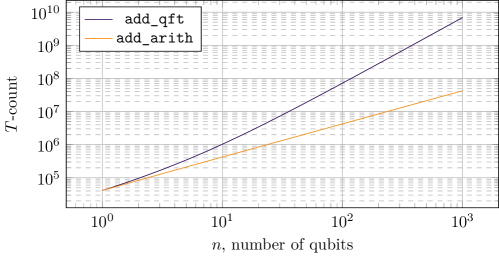
(b) Plot of the $T$-count devised in fig. 20(a) for the two different adder implementations.

Figure 20: Analysis of the $T$-count of the $1$-dimensional wave equation solver quantum implementation with respect to the adder implementation used.

References

- (1)
- mul (2015) 2015. Constructing Large Controlled Nots. https://algassert.com/circuits/2015/06/05/Constructing-Large-Controlled-Nots.html. (2015). Accessed: 2020-03-27.
- ibm (2019a) 2019a. 14-qubit backend: IBM Q team, ”IBM Q 16 Melbourne backend specifications V1.3.0” (2019). (2019). Retrieved from https://quantum-computing.ibm.com.
- qis (2019) 2019. Hamiltonian simulation implementation in qiskit-aqua. https://github.com/Qiskit/qiskit-aqua/blob/master/qiskit/aqua/operators/weighted_pauli_operator.py#L837. (2019). Accessed: 2020-03-27.
- ibm (2019b) 2019b. IBM Quantum Computing. https://www.ibm.com/quantum-computing/. (2019). Accessed: 2020-03-27.
- mel (2019a) 2019a. Melbourne gate specification. https://github.com/Qiskit/ibmq-device-information/tree/master/backends/melbourne/V1#gate-specification. (2019). Accessed: 2020-03-27.
- mel (2019b) 2019b. Melbourne hardware operation execution time. https://github.com/Qiskit/ibmq-device-information/blob/master/backends/melbourne/V1/version_log.md#gate-specification. (2019). Accessed: 2020-03-27.
- sim (2019) 2019. Quantum algorithms for the simulation of Hamiltonian dynamics. https://github.com/njross/simcount. (2019). Accessed: 2020-03-27.
- int (2019) 2019. Quantum computing — Intel Newsroom. https://newsroom.intel.com/press-kits/quantum-computing/. (2019). Accessed: 2020-03-27.
- goo (2019) 2019. Quantum Supremacy Using a Programmable Superconducting Processor. https://ai.googleblog.com/2019/10/quantum-supremacy-using-programmable.html. (2019). Accessed: 2020-03-27.
- Ahokas (2004) Graeme Robert Ahokas. 2004. Improved Algorithms for Approximate Quantum Fourier Transforms and Sparse Hamiltonian Simulations. Master’s thesis. University of Calgary. https://doi.org/10.11575/PRISM/22839
- Arrazola et al. (2018) Juan Miguel Arrazola, Timjan Kalajdzievski, Christian Weedbrook, and Seth Lloyd. 2018. Quantum algorithm for non-homogeneous linear partial differential equations. (09 2018). arXiv:1809.02622v1 http://arxiv.org/abs/1809.02622v1
- Arute et al. (2019) Frank Arute, Kunal Arya, Ryan Babbush, Dave Bacon, Joseph C. Bardin, Rami Barends, Rupak Biswas, Sergio Boixo, Fernando G. S. L. Brandao, David A. Buell, Brian Burkett, Yu Chen, Zijun Chen, Ben Chiaro, Roberto Collins, William Courtney, Andrew Dunsworth, Edward Farhi, Brooks Foxen, Austin Fowler, Craig Gidney, Marissa Giustina, Rob Graff, Keith Guerin, Steve Habegger, Matthew P. Harrigan, Michael J. Hartmann, Alan Ho, Markus Hoffmann, Trent Huang, Travis S. Humble, Sergei V. Isakov, Evan Jeffrey, Zhang Jiang, Dvir Kafri, Kostyantyn Kechedzhi, Julian Kelly, Paul V. Klimov, Sergey Knysh, Alexander Korotkov, Fedor Kostritsa, David Landhuis, Mike Lindmark, Erik Lucero, Dmitry Lyakh, Salvatore Mandrà, Jarrod R. McClean, Matthew McEwen, Anthony Megrant, Xiao Mi, Kristel Michielsen, Masoud Mohseni, Josh Mutus, Ofer Naaman, Matthew Neeley, Charles Neill, Murphy Yuezhen Niu, Eric Ostby, Andre Petukhov, John C. Platt, Chris Quintana, Eleanor G. Rieffel, Pedram Roushan, Nicholas C. Rubin, Daniel Sank, Kevin J. Satzinger, Vadim Smelyanskiy, Kevin J. Sung, Matthew D. Trevithick, Amit Vainsencher, Benjamin Villalonga, Theodore White, Z. Jamie Yao, Ping Yeh, Adam Zalcman, Hartmut Neven, and John M. Martinis. 2019. Quantum supremacy using a programmable superconducting processor. Nature 574 (10 2019), 505–510. Issue 7779. https://doi.org/10.1038/s41586-019-1666-5
- Bamberger et al. (1977) Alain Bamberger, Guy Chavent, and Patrick Lailly. 1977. Une application de la théorie du contrôle à un problème inverse de sismique. Ann. Geophys 33, 1 (1977), 2.
- Bamberger et al. (1979) Alain Bamberger, Guy Chavent, and Patrick Lailly. 1979. About the stability of the inverse problem in 1-D wave equations – application to the interpretation of seismic profiles. Applied Mathematics & Optimization 5 (3 1979), 1–47. Issue 1. https://doi.org/10.1007/BF01442542
- Barenco et al. (1996) Adriano Barenco, Artur Ekert, Kalle-Antti Suominen, and Päivi Törmä. 1996. Approximate Quantum Fourier Transform and Decoherence. (Jan 1996). https://doi.org/10.1103/PhysRevA.54.139 arXiv:quant-ph/9601018v1
- Berry (2010) Dominic W. Berry. 2010. High-order quantum algorithm for solving linear differential equations. (10 2010). https://doi.org/10.1088/1751-8113/47/10/105301 arXiv:1010.2745v2 J. Phys. A: Math. Theor. 47, 105301 (2014).
- Berry et al. (2007) Dominic W. Berry, Graeme Ahokas, Richard Cleve, and Barry C. Sanders. 2007. Efficient Quantum Algorithms for Simulating Sparse Hamiltonians. Communications in Mathematical Physics 270 (1 2007), 359–371. Issue 2. https://doi.org/10.1007/s00220-006-0150-x arXiv:quant-ph/0508139v2 Communications in Mathematical Physics 270, 359 (2007).
- Berry and Childs (2012) Dominic W. Berry and Andrew M. Childs. 2012. Black-box Hamiltonian Simulation and Unitary Implementation. Quantum Info. Comput. 12, 1-2 (01 2012), 29–62. https://doi.org/10.26421/QIC12.1-2 arXiv:0910.4157v4 Quantum Information and Computation 12, 29 (2012).
- Berry et al. (2015b) Dominic W. Berry, Andrew M. Childs, Richard Cleve, Robin Kothari, and Rolando D. Somma. 2015b. Simulating Hamiltonian Dynamics with a Truncated Taylor Series. Physical Review Letters 114 (3 2015). Issue 9. https://doi.org/10.1103/PhysRevLett.114.090502 arXiv:1412.4687v1 Phys. Rev. Lett. 114, 090502 (2015).
- Berry et al. (2015a) Dominic W. Berry, Andrew M. Childs, and Robin Kothari. 2015a. Hamiltonian Simulation with Nearly Optimal Dependence on all Parameters. In 2015 IEEE 56th Annual Symposium on Foundations of Computer Science. 792–809. https://doi.org/10.1109/FOCS.2015.54 arXiv:1501.01715v3 Proceedings of the 56th IEEE Symposium on Foundations of Computer Science (FOCS 2015), pp. 792-809 (2015).
- Berry et al. (2017) Dominic W. Berry, Andrew M. Childs, Aaron Ostrander, and Guoming Wang. 2017. Quantum Algorithm for Linear Differential Equations with Exponentially Improved Dependence on Precision. Communications in Mathematical Physics 356 (12 2017), 1057–1081. Issue 3. https://doi.org/10.1007/s00220-017-3002-y arXiv:1701.03684v2 Communications in Mathematical Physics 356, 1057-1081 (2017).
- Bravo-Prieto et al. (2019) Carlos Bravo-Prieto, Ryan LaRose, M. Cerezo, Yigit Subasi, Lukasz Cincio, and Patrick J. Coles. 2019. Variational Quantum Linear Solver: A Hybrid Algorithm for Linear Systems. (09 2019). arXiv:1909.05820v1 http://arxiv.org/abs/1909.05820v1
- Cao et al. (2018) Yudong Cao, Jonathan Romero, Jonathan P. Olson, Matthias Degroote, Peter D. Johnson, Mária Kieferová, Ian D. Kivlichan, Tim Menke, Borja Peropadre, Nicolas P. D. Sawaya, Sukin Sim, Libor Veis, and Alán Aspuru-Guzik. 2018. Quantum Chemistry in the Age of Quantum Computing. (12 2018). arXiv:1812.09976v2 http://arxiv.org/abs/1812.09976v2
- Childs and Kothari (2011) Andrew M. Childs and Robin Kothari. 2011. Simulating Sparse Hamiltonians with Star Decompositions. In Theory of Quantum Computation, Communication, and Cryptography. Springer Berlin Heidelberg, 94–103. https://doi.org/10.1007/978-3-642-18073-6_8 arXiv:1003.3683v2 Theory of Quantum Computation, Communication, and Cryptography (TQC 2010), Lecture Notes in Computer Science 6519, pp. 94-103 (2011).
- Childs and Liu (2019) Andrew M. Childs and Jin-Peng Liu. 2019. Quantum spectral methods for differential equations. (01 2019). arXiv:1901.00961v1 http://arxiv.org/abs/1901.00961v1
- Childs et al. (2020) Andrew M. Childs, Jin-Peng Liu, and Aaron Ostrander. 2020. High-precision quantum algorithms for partial differential equations. (Feb 2020). arXiv:2002.07868v1 http://arxiv.org/abs/2002.07868v1
- Childs et al. (2018) Andrew M. Childs, Dmitri Maslov, Yunseong Nam, Neil J. Ross, and Yuan Su. 2018. Toward the first quantum simulation with quantum speedup. Proceedings of the National Academy of Sciences 115 (09 2018), 9456–9461. Issue 38. https://doi.org/10.1073/pnas.1801723115 arXiv:1711.10980v1 Proceedings of the National Academy of Sciences 115, 9456-9461 (2018).
- Childs et al. (2019) Andrew M. Childs, Yuan Su, Minh C. Tran, Nathan Wiebe, and Shuchen Zhu. 2019. A Theory of Trotter Error. (Dec 2019). arXiv:1912.08854v1 http://arxiv.org/abs/1912.08854v1
- Childs and Wiebe (2012) Andrew M. Childs and Nathan Wiebe. 2012. Hamiltonian Simulation Using Linear Combinations of Unitary Operations. (02 2012). https://doi.org/10.26421/QIC12.11-12 arXiv:1202.5822v1 Quantum Information and Computation 12, 901-924 (2012).
- Cleve and Watrous (2000) Richard Cleve and John Watrous. 2000. Fast parallel circuits for the quantum Fourier transform. (06 2000). arXiv:quant-ph/0006004v1 http://arxiv.org/abs/quant-ph/0006004v1
- Coles et al. (2018) Patrick J. Coles, Stephan Eidenbenz, Scott Pakin, Adetokunbo Adedoyin, John Ambrosiano, Petr Anisimov, William Casper, Gopinath Chennupati, Carleton Coffrin, Hristo Djidjev, David Gunter, Satish Karra, Nathan Lemons, Shizeng Lin, Andrey Lokhov, Alexander Malyzhenkov, David Mascarenas, Susan Mniszewski, Balu Nadiga, Dan O’Malley, Diane Oyen, Lakshman Prasad, Randy Roberts, Phil Romero, Nandakishore Santhi, Nikolai Sinitsyn, Pieter Swart, Marc Vuffray, Jim Wendelberger, Boram Yoon, Richard Zamora, and Wei Zhu. 2018. Quantum Algorithm Implementations for Beginners. (04 2018). arXiv:1804.03719v1 http://arxiv.org/abs/1804.03719v1
- Costa et al. (2019) Pedro C. S. Costa, Stephen Jordan, and Aaron Ostrander. 2019. Quantum algorithm for simulating the wave equation. Physical Review A 99 (1 2019). Issue 1. https://doi.org/10.1103/PhysRevA.99.012323 arXiv:1711.05394v1 Phys. Rev. A 99, 012323 (2019).
- Cuccaro et al. (2004) Steven A. Cuccaro, Thomas G. Draper, Samuel A. Kutin, and David Petrie Moulton. 2004. A new quantum ripple-carry addition circuit. (10 2004). arXiv:quant-ph/0410184v1 http://arxiv.org/abs/quant-ph/0410184v1
- Draper (2000) Thomas G. Draper. 2000. Addition on a Quantum Computer. (08 2000). arXiv:quant-ph/0008033v1 http://arxiv.org/abs/quant-ph/0008033v1
- Farhi et al. (2014) Edward Farhi, Jeffrey Goldstone, and Sam Gutmann. 2014. A Quantum Approximate Optimization Algorithm. (Nov 2014). arXiv:1411.4028v1 http://arxiv.org/abs/1411.4028v1
- Fowler et al. (2012) Austin G. Fowler, Matteo Mariantoni, John M. Martinis, and Andrew N. Cleland. 2012. Surface codes: Towards practical large-scale quantum computation. (2012). https://doi.org/10.1103/PhysRevA.86.032324 arXiv:quant-ph/1208.0928v2
- García-Ripoll (2019) Juan José García-Ripoll. 2019. Quantum-inspired algorithms for multivariate analysis: from interpolation to partial differential equations. (09 2019). arXiv:1909.06619v1 http://arxiv.org/abs/1909.06619v1
- Gilyén et al. (2018) András Gilyén, Yuan Su, Guang Hao Low, and Nathan Wiebe. 2018. Quantum singular value transformation and beyond: exponential improvements for quantum matrix arithmetics. (06 2018). arXiv:1806.01838v1 http://arxiv.org/abs/1806.01838v1
- Häner et al. (2016) Thomas Häner, Martin Roetteler, and Krysta M. Svore. 2016. Factoring using 2n+2 qubits with Toffoli based modular multiplication. (11 2016). arXiv:1611.07995v2 http://arxiv.org/abs/1611.07995v2 Quantum Information and Computation, Vol. 17, No. 7 & 8 (2017).
- Harrow et al. (2009) Aram W. Harrow, Avinatan Hassidim, and Seth Lloyd. 2009. Quantum Algorithm for Linear Systems of Equations. Physical Review Letters 103 (10 2009). Issue 15. https://doi.org/10.1103/PhysRevLett.103.150502 arXiv:0811.3171v3 Phys. Rev. Lett. vol. 15, no. 103, pp. 150502 (2009).
- Huang et al. (2019) Hsin-Yuan Huang, Kishor Bharti, and Patrick Rebentrost. 2019. Near-term quantum algorithms for linear systems of equations. (Sep 2019). arXiv:1909.07344v2 http://arxiv.org/abs/1909.07344v2
- Kerenidis and Prakash (2017) Iordanis Kerenidis and Anupam Prakash. 2017. Quantum gradient descent for linear systems and least squares. (04 2017). arXiv:1704.04992v3 http://arxiv.org/abs/1704.04992v3
- Kerenidis and Prakash (2018) Iordanis Kerenidis and Anupam Prakash. 2018. A Quantum Interior Point Method for LPs and SDPs. (08 2018). arXiv:1808.09266v1 http://arxiv.org/abs/1808.09266v1
- Kieferova et al. (2018) Maria Kieferova, Artur Scherer, and Dominic Berry. 2018. Simulating the dynamics of time-dependent Hamiltonians with a truncated Dyson series. (05 2018). arXiv:1805.00582v1 http://arxiv.org/abs/1805.00582v1 Only eprint on arXiv.
- Kim and Choi (2018) Taewan Kim and Byung-Soo Choi. 2018. Efficient decomposition methods for controlled-Rnusing a single ancillary qubit. Scientific Reports 8, 1 (03 Apr 2018), 5445. https://doi.org/10.1038/s41598-018-23764-x
- Leyton and Osborne (2008) Sarah K. Leyton and Tobias J. Osborne. 2008. A quantum algorithm to solve nonlinear differential equations. (12 2008). arXiv:0812.4423v1 http://arxiv.org/abs/0812.4423v1
- Low (2018) Guang Hao Low. 2018. Hamiltonian simulation with nearly optimal dependence on spectral norm. (07 2018). arXiv:1807.03967v1 http://arxiv.org/abs/1807.03967v1
- Low and Chuang (2016) Guang Hao Low and Isaac L. Chuang. 2016. Hamiltonian Simulation by Qubitization. (10 2016). arXiv:1610.06546v2 http://arxiv.org/abs/1610.06546v2 Only available as eprint, no journal publication.
- Low and Chuang (2017a) Guang Hao Low and Isaac L. Chuang. 2017a. Hamiltonian Simulation by Uniform Spectral Amplification. (07 2017). arXiv:1707.05391v1 http://arxiv.org/abs/1707.05391v1 Only available as eprint. No journal publication.
- Low and Chuang (2017b) Guang Hao Low and Isaac L. Chuang. 2017b. Optimal Hamiltonian Simulation by Quantum Signal Processing. Physical Review Letters 118 (1 2017). Issue 1. https://doi.org/10.1103/PhysRevLett.118.010501 arXiv:1606.02685v2 Phys. Rev. Lett. 118, 010501 (2017).
- Lubasch et al. (2019) Michael Lubasch, Jaewoo Joo, Pierre Moinier, Martin Kiffner, and Dieter Jaksch. 2019. Variational Quantum Algorithms for Nonlinear Problems. (Jul 2019). arXiv:1907.09032v2 http://arxiv.org/abs/1907.09032v2
- Pino et al. (2020) Juan M. Pino, Joan M. Dreiling, Caroline. Figgatt, John P. Gaebler, Steven A. Moses, Charles H. Baldwin, Michael Foss-Feig, David Hayes, K. Mayer, Ciarán Ryan-Anderson, and Brian Neyenhuis. 2020. Demonstration of the QCCD trapped-ion quantum computer architecture. (Mar 2020). arXiv:2003.01293v2 http://arxiv.org/abs/2003.01293v1
- Ross and Selinger (2014) Neil J Ross and Peter Selinger. 2014. Optimal ancilla-free Clifford+ T approximation of z-rotations. arXiv preprint arXiv:1403.2975 (2014).
- Scherer et al. (2017) Artur Scherer, Benoît Valiron, Siun-Chuon Mau, Scott Alexander, Eric van den Berg, and Thomas E. Chapuran. 2017. Concrete resource analysis of the quantum linear-system algorithm used to compute the electromagnetic scattering cross section of a 2D target. Quantum Information Processing 16 (3 2017). Issue 3. https://doi.org/10.1007/s11128-016-1495-5 arXiv:1505.06552v2 Quantum Inf Process (2017) 16: 60.
- Shao and Xiang (2020) Changpeng Shao and Hua Xiang. 2020. Row and column iteration methods to solve linear systems on a quantum computer. Phys. Rev. A 101 (Feb 2020), 022322. Issue 2. https://doi.org/10.1103/PhysRevA.101.022322
- Shende and Markov (2008) Vivek V. Shende and Igor L. Markov. 2008. On the CNOT-cost of TOFFOLI gates. (2008). arXiv:quant-ph/0803.2316
- Shmoys et al. (2014) David Shmoys, Dominic W. Berry, Andrew M. Childs, Richard Cleve, Robin Kothari, and Rolando D. Somma. 2014. Exponential improvement in precision for simulating sparse Hamiltonians. In Proceedings of the 46th Annual ACM Symposium on Theory of Computing - STOC 14. 283–292. https://doi.org/10.1145/2591796.2591854 arXiv:1312.1414v2 Proceedings of the 46th ACM Symposium on Theory of Computing (STOC 2014), pp. 283-292 (2014).
- Srivastava and Sundararaghavan (2018) Siddhartha Srivastava and Veera Sundararaghavan. 2018. Box algorithm for the solution of differential equations on a quantum annealer. (12 2018). arXiv:1812.10572v2 http://arxiv.org/abs/1812.10572v2
- Suzuki (1986) Masuo Suzuki. 1986. Quantum statistical monte carlo methods and applications to spin systems. Journal of Statistical Physics 43 (6 1986), 883–909. Issue 5-6. https://doi.org/10.1007/BF02628318
- Suzuki (1990) Masuo Suzuki. 1990. Fractal decomposition of exponential operators with applications to many-body theories and Monte Carlo simulations. Physics Letters A 146 (6 1990), 319–323. Issue 6. https://doi.org/10.1016/0375-9601(90)90962-N
- Thapliyal and Ranganathan (2017) Himanshu Thapliyal and Nagarajan Ranganathan. 2017. Design of Efficient Reversible Logic Based Binary and BCD Adder Circuits. (12 2017). https://doi.org/10.1145/2491682 arXiv:1712.02630v1 J. Emerg. Technol. Comput. Syst. 9 (2013) 17:1-17:31.
- Todorova and Steijl (2020) Blaga N. Todorova and René Steijl. 2020. Quantum algorithm for the collisionless Boltzmann equation. J. Comput. Phys. 409 (5 2020), 109347. https://doi.org/10.1016/j.jcp.2020.109347
- Vazquez (2018) Almudena Carrera Vazquez. 2018. Quantum Algorithm for Solving Tri-Diagonal Linear Systems of Equations. Master’s thesis. ETH Zürich.
- Vedral et al. (1996) Vlatko Vedral, Adriano Barenco, and Artur Ekert. 1996. Quantum networks for elementary arithmetic operations. Physical Review A 54, 1 (Jul 1996), 147–153. https://doi.org/10.1103/physreva.54.147
- Xin et al. (2018) Tao Xin, Shijie Wei, Jianlian Cui, Junxiang Xiao, Iñigo Arrazola, Lucas Lamata, Xiangyu Kong, Dawei Lu, Enrique Solano, and Guilu Long. 2018. A Quantum Algorithm for Solving Linear Differential Equations: Theory and Experiment. (07 2018). arXiv:1807.04553v1 http://arxiv.org/abs/1807.04553v1
- Xu et al. (2019) Xiaosi Xu, Jinzhao Sun, Suguru Endo, Ying Li, Simon C. Benjamin, and Xiao Yuan. 2019. Variational algorithms for linear algebra. (09 2019). arXiv:1909.03898v1 http://arxiv.org/abs/1909.03898v1