Abstract

Macroscopic growth laws describe in an effective way the underlying complex dynamics of the spreading of infections, as in the case of CoviD-19, where the counting of the cumulative number $N(t)$ of detected infected individuals is a generally accepted variable to understand the epidemic phase. However $N(t)$ does not take into account the unknown number of asymptomatic cases $A(t)$. The considered model of CoviD-19 spreading is based on a system of coupled differential equations, which include the dynamics of the spreading among symptomatic and asymptomatic individuals and the strong containment effects due to the social isolation. The solution has ben compared with $N(t)$, determined by a single differential equation with no explicit reference to $A(t)$, showing the equivalence of the two methods. The model is applied to Covid-19 spreading in Italy where a transition from an exponential behavior to a Gompertz growth for $N(t)$ has been observed in more recent data. The information contained in the time series $N(t)$ turns out to be reliable to understand the epidemic phase, although it does not describe the total infected population. The asymptomatic population is larger than the symptomatic one in the fast growth phase of the spreading.

I Introduction

There is an impressive number of experimental verifications, in many different scientific sectors, that coarse-grain properties of systems, with simple laws with respect to the fundamental microscopic algorithms, emerge at different levels of magnification providing important tools for explaining and predicting new phenomena.

For example, the Gompertz law (GL) GL , initially applied to human mortality tables (i.e. aging), describes tumor growth steel ; norton , kinetics of enzymatic reactions, oxygenation of hemoglobin, intensity of photosynthesis as a function of CO2 concentration, drug dose-response curve, dynamics of growth, (e.g., bacteria, normal eukaryotic organisms). Analogously, the Logistic Law (LL) LL has been applied in population dynamics, in economics, in material science and in many other sectors.

The ability of macroscopic growth laws in describing the underlying complex dynamics is sometime surprising.

A clear and timely example is given by the infection spreading (Coronavirus oms1 ; oms2 in particular), where different Governments impose strong containment efforts on the basis of the mortality rate and of the growth rate of the cumulative total number of detected infected people $N(t)$ at time $t$, which has a strong impact on the national health systems.

However, there is a large number of infected people without any symptoms who contribute to the disease spreading but are not explicitly taken into account in $N(t)$, since not detected.

More precisely, a macroscopic growth law for $N(t)$ is solution of the general differential equation

$$\frac{dN}{dt}=\alpha_{eff}(t)N(t),$$ (1)

where $\alpha_{eff}(t)$ is the specific growth rate at time $t$. For example, if $\alpha_{eff(t)}=$constant one obtains the exponential behavior. Various growth patterns have been very recently applied to the time evolution of the CoviD-19 infection np7 ; np8 ; np9 ; np10 ; np11 ; np12 ; np13 . On the other hand, by using the previous equation to describe the epidemic phase, the cumulative number of asymptomatic infected individuals, $A(t)$, seems completely neglected. Indeed, the second term of the equation depends on $N(t)$ only.

For the CoviD-19 infection, since $A(t)$ is unknown, many Governments have correctly applied strong constraints to slow down the spreading: social isolation, information on the localization of infected individuals and the use of a very large number of medical swabs.

However, the question arises: is the information obtained by monitoring $N(t)$ reliable in understanding the epidemic phase?

By a simple model of the interaction between the symptomatic cumulative detected population $N(t)$ and the asymptomatic one, $A(t)$, we discuss how the effective coarse-grain equation (1) takes into account the asymptomatic population in the transient phase of the spreading. Moreover one gets useful indications on the number of asymptomatic individuals and on the effective lethality.

In Sec.1 different macroscopic growth laws are applied to the cumulative number of detected infected individuals in China, South Korea and Italy, where the containment effort started earlier, to describe the phases of the spreading. A simple dynamical model where the asymptomatic population and the isolation effect play an important role is discussed in Sec.2. The results are in Sec.3 and Sec.4 is devoted to comments and conclusions.

II Infection spreading phases: macroscopic description

The macroscopic growth laws in eq. (1), can be classified by considering the time derivative of $\alpha_{eff}$, as shown in ref. cast1 ; cast2 . For example the GL and the LL are in the, so called, universality class U2 cast1 , where $d\alpha_{eff}/dt=a_{1}\alpha+a_{2}\alpha^{2}$. Moreover, the Gompertz and the logistic equations can be written in a different way, which clarifies the feedback effect of the increasing population , i.e.

$$\frac{1}{N(t)}\frac{dN(t)}{dt}=-k_{g}\;\ln\frac{N(t)}{N_{\infty}^{g}}\qquad\text{Gompertz}\;,$$ (2)

$$\frac{1}{N(t)}\frac{dN(t)}{dt}=k_{l}\left(1-\frac{N(t)}{N_{\infty}^{l}}\right)\qquad\text{logistic}$$ (3)

where $k_{g}$, $N_{\infty}^{g}$, $k_{l}$ and $N_{\infty}^{l}$ are constants.

In the GL and in the LL, $k_{g}\ln(N_{\infty}^{g})$ and $k_{l}$ are respectively the initial exponential rates and the other terms determine their slowdown.

The comparison of the growth laws, solutions of the previous differential equations, with the data on the cumulative number of infected individuals is reported in fig. 1 for China, showing that the coronavirus spreading has three phases: an initial exponential behavior, followed by a Gompertz one and a final logistic phase. For South Korea, after the three phases, the spreading seems to restart (see fig. 2). Italy is still in the Gompertz growth phase (see fig. 3).

The previous equations neglect the large (undetected) asymptomatic population and the isolation effects, since they concern the time evolution of $N(t)$ only. However, a simple model in the next section shows that the GL takes into account a more complex underlying dynamics. The analysis can be repeated for the LL.

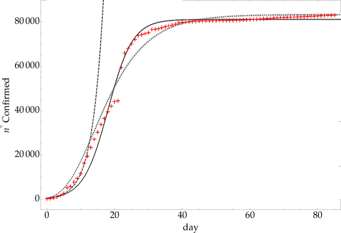
Figure 1: Comparison of the growth laws with the data of the cumulative number of infected individuals in China: continuous line si the logistic curve, dotted line the Gompertz, the dashed one the exponential. Time zero corresponds to the initial day - 22/01.

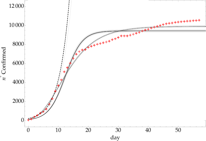
Figure 2: Comparison of the growth laws with the data of the cumulative number of infected individuals in South Korea: continuous line si the logistic curve, dotted line the Gompertz, the dashed one the exponential. Time zero corresponds to the initial day - 20/02.

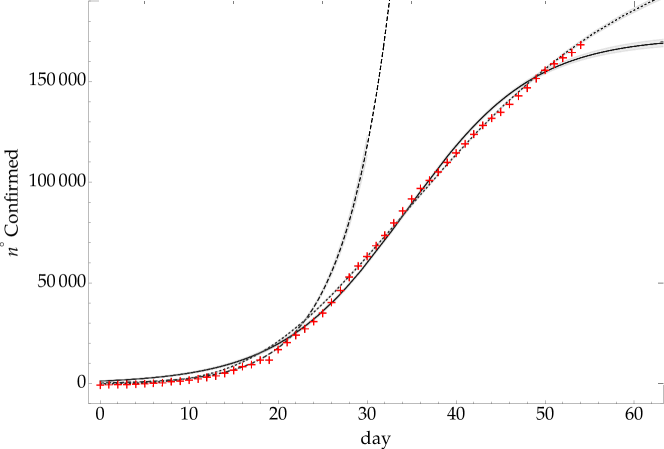
Figure 3: Comparison of the growth laws with the data of the cumulative number of infected individuals in Italy: continuous line si the logistic curve, dotted line the Gompertz, the dashed one the exponential. Time zero corresponds to the initial day - 22/02.

III A simple model: asymptomatic population and containment effects

In the model, we call $T(t)$ the cumulative total number of infected people, which is the sum of the number of the cumulative detected infected individuals $N(t)$ and of the asymptomatic ones $A(t)$: $T(t)=N(t)+A(t)$.

In the data of $N(t)$ the number of dead and of healed people is included, since they have been previously infected. In the fast growing phase, their total number is much smaller than $N(t)$ and therefore they are not included in the dynamics (the re-infection is considered very unlikely). The previous condition defines the transient phase.

Therefore one has to take into account the rates of the following processes ($n$ = detected infected person, $a$ = asymptomatic infected person): $n\rightarrow n+n$, $a\rightarrow n+a$, $n\rightarrow n+a$, $a\rightarrow a+a$ with rates $c_{1}(t)$, $c_{2}(t)$, $c_{3}(t)$, $c_{4}(t)$ respectively.

Accordingly, the corresponding mean field equations are

$$\frac{dN(t)}{dt}=c_{1}(t)N(t)+c_{2}(t)A(t),$$ (4)

$$\frac{dA(t)}{dt}=c_{3}(t)N(t)+c_{4}(t)A(t).$$ (5)

The functions $c_{i}(t)$, $i=1,4$, describe the damping effects due to the containment effort and we assume they have an exponential decreasing behavior:

$$c_{i}(t)\simeq e^{-\lambda t}$$ (6)

i.e. the rates of the dynamical processes decrease in time due to social isolation and other external constraints. This effect should be independent on the status of the infected individual (n or a). On the other hand, in the processes involving a symptomatic individual, he/she is (or should be) rapidly detected, together with those who belong to his/her chain of infection transmission, independently on their symptomatic or asymptomatic condition. Therefore the rate of the processes involving infected persons should be suppressed with respect to the transmission rate among asymptomatic persons, which is “invisible”.

In other terms, one expects that, in the transient phase, the rate of the process among asymptomatic individuals only, $a\rightarrow a+a$, decreases slowly than the other ones. As a first step, one assumes that the functions $c_{1}(t)$, $c_{2}(t)$, $c_{3}(t)$, $c_{4}(t)$ are given by

$$c_{1}(t)=c_{1}^{0}e^{-\lambda_{1}t},\phantom{...}c_{2}(t)=c_{2}^{0}e^{-\lambda_{1}t},\phantom{...}c_{3}(t)=c_{3}^{0}e^{-\lambda_{1}t},\phantom{...}c_{4}(t)=c_{4}^{0}e^{-\lambda_{2}t},$$ (7)

with $\lambda_{2}<\lambda_{1}$ and $c_{i}^{0}>0$. The coefficients $c_{i}^{0}$ are the initial rates and $\lambda_{1}$, $\lambda_{2}$ parameterize their reduction due to the isolation conditions.

it is an effective way to take into account the dynamics in eqs. (4, 5, 7).

To clarify that the solution of eq.(2) takes into account, in an effective way, the dynamics in eqs. (4, 5, 7), the system is analytically solved (see appendix) for $\lambda_{1}=\lambda_{2}$. For $\lambda_{2}<\lambda_{1}$ there is no analytical solution and the numerical one will be compared with the Italian data and the previous GL fit in the next section.

IV Results

The Gompertz fit (from eq. (2)) of Italian data is compared with the numerical solution of the dynamical system (4, 5, 7) with $\lambda_{2}<\lambda_{1}$ in fig. 4. The two curves are well compatible, indicating that the interaction between symptomatic and asymptomatic populations is contained in eq. (2) in an effective way. Moreover the solution of the system gives an estimate of the asymptomatic population, plotted in fig. 5.

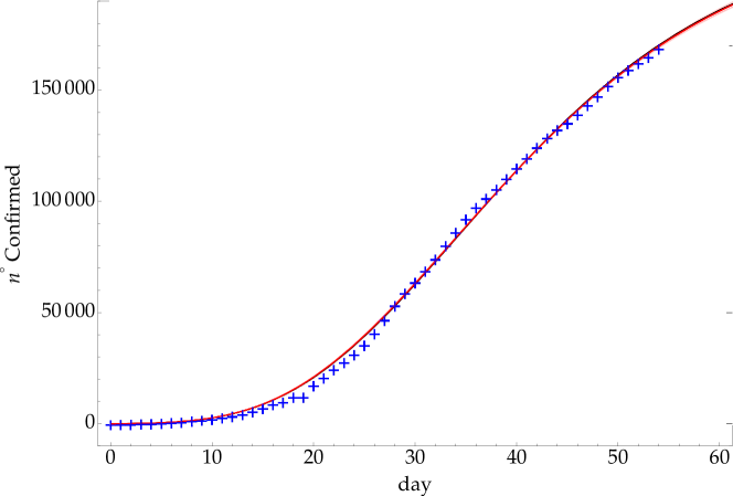
Figure 4: Cumulative number of infected individuals in Italy from February 22nd (day 0) to April the 16th. The GL fit (red) and the solution of the system in eq. (4, 5, 7) (black) are plotted versus the observed data. The parameters are: $N(0)=62$, $A(0)=N(0)$, $c_{1}^{0}=0.23$, $c_{2}^{0}=0.26$, $c_{3}^{0}=0.24$, $c_{4}^{0}=0.32$, $\lambda_{1}=0.0732$, $\lambda_{2}=0.045$. The two curves overlap.

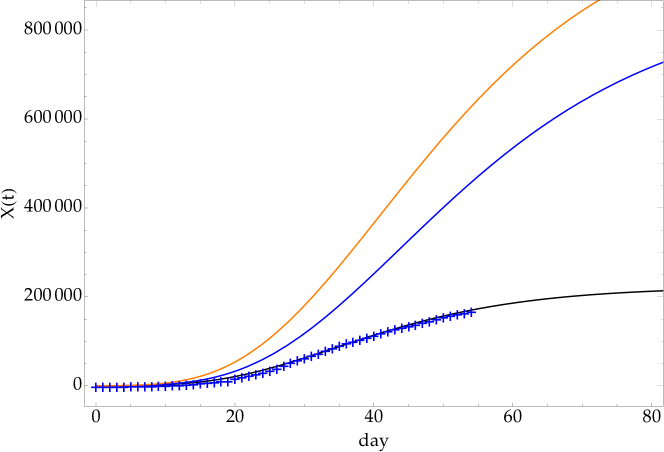
Figure 5: Cumulative number of infected individuals in Italy from February 22nd(day 0) to March 22nd. The solution of the system in eqs. (4, 5, 7) are plotted: detected in black, asymptomatic in blue, total in orange.

The previous analysis clearly suggests that:

• the curve $N(t)$ takes into account the dynamics of the asymptomatic individuals;

• in the fast growing phase there is a large asymptomatic population: to stop the infection spreading the strong social isolation is the best method;

• the time evolution of $N(t)$ is an effective macroscopic growth laws solution of eq. 2 for Italy, completely consistent with the system in eqs. (4, 5, 7).

In this respect the choice of monitoring the time evolution of $N(t)$ to understand the epidemic phase is reliable, since the underling dynamics is included in the time dependence of $\alpha_{eff}$ in eq. (1). This is probably related to the result that a general classification of the growth laws depends on the time derivative of $\alpha_{eff}$ cast1 ; cast2 .

On the other hand, the system of differential equations give more information than the single equation for $N(t)$. In particular, the ratio, $R(t)$ (see appendix), between symptomatic and asymptomatic populations is plotted as a function of time in fig. 6. Moreover, one can evaluate in a more reliable way the lethality of the infection, defined as the ratio of the number of dead individuals and the total number of infected ones. The italian lethality is $13\%$ neglecting the asymptomatic population, but, in our model, its value reduces to $\simeq 3\%$ considering the total infected population.

Figure 6: Ratio between asymptomatic and symptomatic populations.

V Comments and Conclusions

The model in eqs. (4, 5, 7) is a simplified version of a more complex dynamics net1 ; net2 and can be improved including other specific populations smaller .

Different analyses of the CoviD-19 spreading predict a large asymptomatic population. In ref. np10 the number of asymptomatic individuals in Italy on March 12th turns out to be more than 100.000 versus a symptomatic detected population of about 12.000. Our analysis suggests an asymptotic population of about 27500 individuals on March 12th, 76000 on March 19th and 129000 on March 24th. In ref. lan , the outbreak in Italy has been estimated, giving a ratio of about 1:3 between symptomatic and asymptomatic individuals on February 29Th. The evaluation of the asymptomatic population is a difficult task and the results are strongly model dependent.

Macroscopic laws in eq. (1) include the dynamics of the infection with the advantage of a reduction of the free parameters: the simple system in eqs. (4, 5, 7) has in principle 5 parameters plus 2 initial conditions, but the Gompertz curve has 2 parameters and 1 initial condition.

The reliability of $N(t)$ as an index of the spreading has been checked by a devoted analysis, including the crucial effects of the social isolation and the role of the asymptomatic individuals.

A further confirmation of this conclusion comes from the direct comparison between the daily rate $N(t+1)-N(t)$ and the corresponding mortality one, reported in figs. (7,8), which shows that the time evolution of $N(t)$ anticipates the other by about 8 days.

Figure 7: Confirmed daily rate.

Figure 8: Mortality daily rate.

It should be clear that the previous analysis implicitly assumes that the protocol concerning the detection of infected individuals, as for example the number of medical swabs (per day), does not change in time. Indeed, a modification in the detecting protocol (as in the Chinese case) or the sudden, strong, variation in the number of swabs could mimic an increase or a decrease in $N(t)$ of not dynamical origin.

VI Acknowledgements

P.C. thanks V. Latora for useful comments and suggestions.

VII Appendix

Let us consider the system of differential equations

$$\begin{cases}\displaystyle\frac{dN(t)}{dt}=c_{1}(t)N(t)+c_{2}(t)A(t)\\ \\ \displaystyle\frac{dA(t)}{dt}=c_{3}(t)N(t)+c_{4}(t)A(t)\end{cases}\;,$$ (8)

with

$$c_{i}=c_{i}^{0}\;e^{-\lambda\;t}\;,$$ (9)

.

It can be solved by defining the ratio

$$R(t)\equiv\frac{A(t)}{N(t)}\;,$$ (10)

which satisfies the equation

$$\frac{dR(t)}{dt}=e^{-\lambda\;t}\left[c_{3}^{0}-R(t)\;\left[c_{1}^{0}-c_{4}^{0}+c_{2}^{0}\;R(t)\right]\right]\;.$$ (11)

The analytical solution of the previous eq. (11) is

$$R(t)=\frac{R_{+}-R_{-}\;\frac{R_{0}-R_{+}}{R_{0}-R_{-}}\;e^{-\frac{c_{2}^{0}}{\lambda}\;(R_{+}-R_{-})\;\left(1-e^{-\lambda\;t}\right)}}{1-\frac{R_{0}-R_{+}}{R_{0}-R_{-}}\;e^{-\frac{c_{2}^{0}}{\lambda}\;(R_{+}-R_{-})\;\left(1-e^{-\lambda\;t}\right)}}\;,$$ (12)

where

$$R_{\pm}=\frac{1}{2}\left[-\frac{c_{1}^{0}-c_{4}^{0}}{c_{2}^{0}}\pm\sqrt{\left(\frac{c_{1}^{0}-c_{4}^{0}}{c_{2}^{0}}\right)^{2}+\frac{4\;c_{3}^{0}}{c_{2}^{0}}}\;\right]$$ (13)

and $R_{0}=R(t=0)=A_{0}/N_{0}$, being $N_{0}$ and $A_{0}$ the number of detected and asymptomatic infected individuals at the initial time respectively.

Putting $A(t)=R(t)\;N(t)$ in eq. (8) it turns out that

$$N(t)=\frac{N_{0}\;e^{\frac{c_{1}^{0}+c_{2}^{0}\;R_{+}}{\lambda}\left(1-e^{-\lambda t}\right)}}{R_{-}-R_{+}}\;\left[(R_{0}-R_{+})\;e^{\frac{c_{2}^{0}}{\lambda}(R_{-}-R_{+})\left(1-e^{-\lambda t}\right)}-R_{0}+R_{-}\right]\;,$$ (14)

and

$$A(t)=\frac{N_{0}\;e^{\frac{c_{1}^{0}+c_{2}^{0}\;R_{+}}{\lambda}\left(1-e^{-\lambda t}\right)}}{R_{+}-R_{-}}\Bigg{[}R_{-}\;(R_{+}-R_{0})\;e^{\frac{c_{2}^{0}(R_{-}-R_{+})}{\lambda}\left(1-e^{-\lambda t}\right)}+R_{+}(R_{0}-R_{-})\Bigg{]}\;.$$ (15)

Finally, for the specific case $c_{3}^{0}=c_{1}^{0}$ and $c_{2}^{0}=c_{4}^{0}=k\;c_{1}^{0}$, with $k$ some constant,

$$N(t)=\frac{N_{0}}{k+1}\;\left((k\;R_{0}+1)e^{\frac{c_{1}^{0}(k+1)}{\lambda}\;\left(1-e^{-\lambda t}\right)}+k(1-R_{0})\right)\;,$$ (16)

$$A(t)=\frac{N_{0}}{k+1}\;\left((k\;R_{0}+1)\;e^{\frac{c_{1}^{0}(k+1)}{\lambda}\;\left(1-e^{-\lambda t}\right)}+R_{0}-1\right)\;,$$ (17)

and

$$R(t)=1+\frac{(R_{0}-1)(1+k)}{(k\;R_{0}+1)\;e^{\frac{c_{1}^{0}\;(k+1)}{\lambda}\;\left(1-e^{-\lambda t}\right)}+k(1-R_{0})}$$ (18)

The typical time dependence of the previous solutions, $N(t)$ and $A(t)$, is plotted in figure 9.

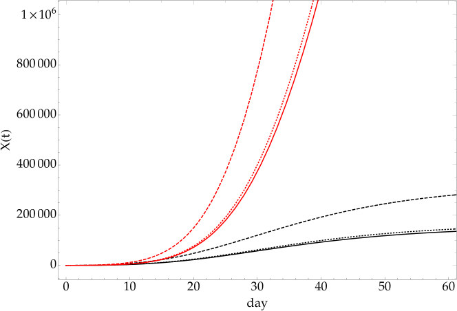
Figure 9: Solution of eq. (8) with $N(0)=62$, $A(0)=N(0)$, $c_{1}^{0}=0.23$, $c_{2}^{0}=0.26$, $c_{3}^{0}=0.24$, $c_{4}^{0}=0.32$. Black curves are for $\lambda=0.0732$, the red ones for $\lambda=0.045$. Continuous curves give the cumulative number of detected infected individuals ($N(t)$), the dotted one correspond to the asymptomatic ones, $A(t)$, and the dashed line is the total.

References

- (1) B. Gompertz, On the nature of the function expressive of the law of human mortality and a new mode of determining life contingencies, Phil. Trans. R. Soc. 115 (1825) 513.
- (2) G.G: Steel, Growth kinetics of tumours, Clarendon Press, Oxford, 1977.
- (3) L. A. Norton, Gompertzian model of human breast cancer growth, Cancer. Res. 48 (1988) 7067.
- (4) P. F. Verhulst, Notice sur la loi que la population poursuit dans son accroissement, Correspondance Mathématique et Physique, 10 (1838) 113.
-
(5)
World Health Organization, Coronavirus disease (COVID-19) outbreak,
https://www.who.int/emergencies/diseases/novel-coronavirus-2019. - (6) World Health Organization, Coronavirus disease (COVID-19) report, https://www.who.int/docs/default-source/ coronaviruse/who-china-joint-mission-on-covid-19-final-report.pdf.
- (7) A. Lai, A. Bergna, C. Acciarri, M. Galli, G. Zehender, Early Phylogenetic Estimate of the Effective Reproduction Number Of Sars-CoV-2, J. Med. Virol. 2020 Feb 25,doi: 10.1002/jmv.25723.
- (8) Y. Chen, Q. Liu, D. Guo, Emerging coronaviruses: Genome structure, replication, and pathogenesis, J. Med.Virol. 92 (2020) 418.
- (9) P.Castorina, A.Iorio and D.Lanteri, Data analysis on Coronavirus spreading by macroscopic growth laws, arXiv:2003.00507, 1 March 2020, in press in INternational Journal Modern Physics C.
- (10) L.Fenga, CoViD19: An Automatic,Semiparametric Estimation Method for the Population Infected in Italy, medRxiv preprint doi: https://doi.org/10.1101/2020.03.14.20036103.
- (11) D.Fanelli and F.Piazza, Analysis and forecast of COVID-19 spreading in China, Italy and France, arXiv:2003.06031, 13 March 2020.
- (12) A.Agosto and P. Giudici, A Poisson Autoregressive Model to Understand COVID-19 Contagion Dynamics, ssrn - abstract-id=3551626.
- (13) S.Bialek et al, CDC COVID-19 Response Team, Severe Outcomes Among Patients with Coronavirus Disease 2019 (COVID-19) - United States, February 12 - March 16, 2020. MMWR Morb Mortal Wkly Rep. ePub: 18 March 2020.
- (14) P. Castorina, P. P. Delsanto, C. Guiot, Classification Scheme for Phenomenological Universalities in Growth Problems in Physics and Other Sciences, Phys. Rev. Lett. 96 (2006) 188701.
- (15) P. Castorina and P. Blanchard, Unified approach to growth and aging in biological, technical and biotechnical systems, SpringerPlus 1 (2012).
- (16) S. A. Herzog, S. Blaizot and Niel Hens, Mathematical models used to inform study design or surveillance systems in infectious diseases: a systematic review, BMC Infectious Diseases 17 (2017) 775.
- (17) N. C. Grassly and C. Fraser, Mathematical models of infectious disease transmission, Nature Reviews Microbiology 6 (2008) 477.
- (18) V. Zlatic, I. Barjasic, A. Kadovic, H. Stefancic and A. Gabrielli, Bi-stability of SUDR+K model of epidemics and test kits applied to COVID-19, arXiv: 2003.08479, March 18th 2020.
- (19) A.R.Tuite, V. Ng, E.Rees and D.Fisman, Estimation of COVID-19 outbreak size in Italy, Lancet Infect Dis 2020 Published Online March 19, 2020, doi.org/10.1016/ S1473-3099(20)30227-9