Polynomial graph filters of multiple shifts and distributed implementation of inverse filtering

Abstract

Polynomial graph filters and their inverses play important roles in graph signal processing. In this paper, we introduce the concept of multiple commutative graph shifts and polynomial graph filters, which could play similar roles in graph signal processing as the one-order delay and finite impulse response filters in classical multi-dimensional signal processing. We implement the filtering procedure associated with a polynomial graph filter of multiple shifts at the vertex level in a distributed network on which each vertex is equipped with a data processing subsystem for limited computation power and data storage, and a communication subsystem for direct data exchange only to its adjacent vertices. In this paper, we also consider the implementation of inverse filtering procedure associated with a polynomial graph filter of multiple shifts, and we propose two iterative approximation algorithms applicable in a distributed network and in a central facility. We also demonstrate the effectiveness of the proposed algorithms to implement the inverse filtering procedure on denoising time-varying graph signals and a dataset of US hourly temperature at $218$ locations.

Keywords: Graph signal processing, polynomial graph filter, inverse filtering, distributed algorithm, distributed network, multivariate Chebyshev polynomial approximation.

1 Introduction

Graph signal processing provides an innovative framework to handle data residing on spatially distributed networks (SDN), such as the wireless sensor networks, smart grids and social network and many other irregular domains, [7, 17, 33, 38, 45, 51]. Graphs provide a flexible tool to model the underlying topology of the networks, and the edges present the interrelationship between data elements. For instance, an edge between two vertices may indicate the availability of a direct data exchanging channel between sensors of a distributed network, the functional connectivity between neural regions in brain, or the correlation between temperature records of neighboring locations. By leveraging graph spectral theory and applied harmonic analysis, graph signal processing has been extensively exploited, and many important concepts in classical signal processing, such as Fourier transform and wavelet filter banks, have been extended to graph setting [7, 16, 30, 33, 36, 37, 38, 45, 47].

Let ${\mathcal{G}}:=(V,E)$ be an undirected and unweighted graph with vertex set $V=\{1,\ldots,N\}$ and edge set $E\subset V\times V$, and define the geodesic distance $\rho(i,j)$ between vertices $i,j\in V$ by the number of edges in a shortest path connecting $i,j\in V$ and set $\rho(i,j)=\infty$ if vertices $i,j\in V$ belong to its different connected components. A graph filter on the graph $\mathcal{G}$ maps one graph signal ${\bf x}=(x(i))_{i\in V}$ linearly to another graph signal ${\bf y}={\bf H}{\bf x}$, and it is usually represented by a matrix ${\bf H}=(H(i,j))_{i,j\in V}$. Graph filters and their implementations are fundamental in graph signal processing, and they have been used in denoising, smoothing, consensus of multi-agent systems, the estimation of time series and many other applications [20, 46, 49, 50]. In the classical signal processing, filters are categorized into two families, finite impulse response (FIR) filters and infinite impulse response (IIR) filters. The FIR concept has been extended to graph filters with the duration of an FIR filter being replaced by the geodesic-width of a graph filter. Here the geodesic-width $\omega({\bf H})$ of a graph filter ${\bf H}=(H(i,j))_{i,j\in V}$ is the smallest nonnegative integer $\omega({\bf H})$ such that $H(i,j)=0$ hold for all $i,j\in V$ with $\rho(i,j)>\omega({\bf H})$ [5, 7, 10, 21, 22].

An elementary graph filter is a graph shift, which has one as its geodesic-width [13, 21, 36, 40]. In this paper, we introduce the concept of multiple commutative graph shifts ${\bf S}_{1},\dots,{\bf S}_{d}$, i.e.,

$${\bf S}_{k}{\bf S}_{k^{\prime}}={\bf S}_{k^{\prime}}{\bf S}_{k},\ 1\leq k,k^{\prime}\leq d,$$ (1.1)

and we consider the implementation of filtering and inverse filtering associated with a polynomial graph filter

$${\bf H}=h({\bf S}_{1},\ldots,{\bf S}_{d})=\sum_{l_{1}=0}^{L_{1}}\cdots\sum_{l_{d}=0}^{L_{d}}h_{l_{1},\dots,l_{d}}{\bf S}_{1}^{l_{1}}\cdots{\bf S}_{d}^{l_{d}},$$ (1.2)

where the polynomial

$$h(t_{1},\ldots,t_{d})=\sum_{l_{1}=0}^{L_{1}}\cdots\sum_{l_{d}=0}^{L_{d}}h_{l_{1},\dots,l_{d}}t_{1}^{l_{1}}\ldots t_{d}^{l_{d}}$$

in variables $t_{1},\cdots,t_{d}$ has polynomial coefficients $h_{l_{1},\dots,l_{d}}$, $0\leq l_{k}\leq L_{k},1\leq k\leq d$. The commutativity of graph shifts ${\bf S}_{1},\dots,{\bf S}_{d}$ guarantees that the polynomial graph filter ${\bf H}$ in (1.2) is independent on equivalent expressions of the multivariate polynomial $h$, and also the well-definedness of their joint spectrum, see Appendix A.3. The concept of commutative graph shifts ${\bf S}_{1},\dots,{\bf S}_{d}$ may play a similar role in graph signal processing as the one-order delay $z_{1}^{-1},\ldots,z_{d}^{-1}$ in classical multi-dimensional signal processing, and in practice graph shifts may have specific features and physical interpretation, see Appendix A and Section 5 for some illustrative examples. We remark that the commutative assumption on graph shifts ${\bf S}_{1},\ldots,{\bf S}_{d}$ is trivial for $d=1$ and polynomial graph filters of a single shift have been widely used in graph signal processing [6, 9, 19, 29, 40, 46, 49].

Polynomial graph filters ${\bf H}$ in (1.2) have geodesic-width $\omega({\bf H})$ no more than the degree $\sum_{k=1}^{d}L_{k}$ of the polynomial $h$. Our study of polynomial graph filters of multiple shifts is mainly motivated by signal processing on time-varying signals, such as video and data collected by a sensor network over a period of time, which carry different correlation characteristics for different dimensions/directions. In such a scenario, graph filters should be designed to reflect spectral characteristic on the vertex domain and also on the temporal domain, hence polynomial graph filters of multiple commutative shifts are preferable, see [26, 33, 38] and also Subsections 5.2 and 5.3. The design of polynomial filters of multiple graph shifts and their inverses with specific features and physical interpretation for engineering applications is beyond the scope of this paper and it will be discussed in our future work. Our discussion is also motivated by directional frequency analysis in [26], feature separation in [12] and graph filtering in [1] for time-varying graph signals.

For polynomial graph filters of a single shift, algorithms have been proposed to implement their filtering procedure in finite steps, with each step including data exchanging between adjacent vertices only, see [6, 19, 41, 46, 49, 50] and also Algorithm 2.1. The first main contribution is to extend the one-hop implementation in Algorithm 2.1 to the filtering procedure associated with polynomial graph filters of multiple shifts, see Algorithm 2.2 in Section 2. Therefore the filtering procedure associated with polynomial graph filters can be implemented on an SDN on which each agent is equipped with a data processing subsystem having limited data storage and computation power, and with a communication subsystem for data exchanging to its adjacent agents.

Inverse filtering associated with the graph filter having small geodesic-width plays an important role in graph signal processing, such as denoising, graph semi-supervised learning, non-subsampled filter banks and signal reconstruction [2, 3, 6, 9, 19, 21, 29, 32, 41, 46]. The challenge arisen in the inverse filtering is on its implementation, as the inverse filter ${\bf H}^{-1}$ usually has full geodesic-width even if the original filter ${\bf H}$ has small geodesic-width. For the case that the filter ${\bf H}$ is strictly positive definite, the inverse filtering procedure ${\bf b}\longmapsto{\bf H}^{-1}{\bf b}$ can be implemented by applying the iterative gradient descent method in a distributed network, see [2, 35, 41] and Remark 3.2. Denote the identity matrix by ${\bf I}$. To consider implementation of inverse filtering of an arbitrary invertible filter ${\bf H}$ with small geodesic-width, in Section 3 we start from selecting a graph filter ${\bf G}$ with small geodesic-width to approximate the inverse filter ${\bf H}^{-1}$ so that the spectral radius of ${\bf I}-{\bf H}{\bf G}$ is strictly less than 1, and then we propose an exponential convergent algorithm (3.5) and (3.6) to implement the inverse filtering procedure with each iteration mainly including two filtering procedures associated with filters ${\bf H}$ and ${\bf G}$, see Theorem 3.1.

For an invertible polynomial graph filter of a single shift, there are several methods to implement the inverse filtering in a distributed network approximately [6, 9, 19, 41, 46], see Remark 4.7. The second main contribution of this paper is that we introduce optimal polynomial filters and multivariate Chebyshev polynomial filters to provide good approximations to the inverse of an invertible polynomial graph filter ${\bf H}$ of multiple shifts, see Section 4. Then, based on the iterative approximation algorithm in Section 3, we propose the iterative optimal polynomial approximation algorithm (4.7) and the iterative Chebyshev polynomial approximation algorithm (4.16) to implement the inverse filtering procedure ${\bf b}\longmapsto{\bf H}^{-1}{\bf b}$, see Theorems 4.2 and 4.4 for their exponential convergence. More importantly, as shown in Algorithms 4.1 and 4.2, each iteration in the proposed iterative algorithms mainly contains two filtering procedures involving data exchanging between adjacent vertices only and hence they can be implemented in a distributed network of large size, where each vertex is equipped with systems for limited data storage, computation power and data exchanging facility to its adjacent vertices.

The paper is organized as follows. In Section 2, we consider distributed implementation of the filtering procedure associated with polynomial graph filters of multiple shifts at the vertex level. In Section 3, we propose an iterative approximation algorithm to implement an inverse filtering procedure. In Section 4, we propose the iterative optimal polynomial approximation algorithm and the iterative Chebyshev polynomial approximation algorithm to implement the inverse filtering procedure associated with a polynomial filter. The effectiveness of these two iterative algorithms to implement the inverse filtering procedure is demonstrated in Section 5. In Appendix A, we introduce two illustrative families of commutative graph shifts on circulant graphs and product graphs respectively, and we define joint spectrum (A.5) of multiple commutative graph shifts, which is crucial for us to develop the iterative algorithms for inverse filtering in Section 4. In Appendix A, we also consider the problem when a graph filter is a polynomial of multiple commutative graph shifts and how to measure the distance between a graph filter and the set of polynomial filters of commutative graph shifts.

2 Polynomial filter and distributed implementation

Algorithm 2.1 Backward iteratively synchronous realization of the filtering procedure ${\bf x}\longmapsto{\bf H}{\bf x}$ for a polynomial filter ${\bf H}=\sum^{L}_{l=0}h_{l}{\bf S}^{l}$ at a vertex $i\in V$.

  Inputs: Polynomial coefficients $h_{0},h_{1},\ldots,h_{L}$, entries $S(i,j),j\in{\mathcal{N}}_{i}$ in the $i$-th row of the shift ${\bf S}$, and the value $x(i)$ of the input signal ${\bf x}=(x(i))_{i\in V}$ at the vertex $i$.

  Initialization: $z^{(0)}(i)=h_{L}x(i)$ and $n=0$.

  1) Send $z^{(n)}(i)$ to its adjacent vertices $j\in{\mathcal{N}}_{i}$ and receive $z^{(n)}(j)$ from its adjacent vertices $j\in{\mathcal{N}}_{i}$.

  2) Update $z^{(n+1)}(i)=h_{L-n-1}x(i)+\sum\limits_{j\in{\mathcal{N}}_{i}}S(i,j)z^{(n)}(j).$

  3) Set $n=n+1$ and return to Step 1) if $n\leq L-1$.

  Output: The value $\tilde{x}(i)=z^{(L)}(i)$ is the output signal ${\bf H}{\bf x}=(\tilde{x}(i))_{i\in V}$ at the vertex $i$.

Let ${\mathcal{G}}=(V,E)$ be a connected, undirected and unweighted graph of order $N$. Graph shifts ${\bf S}$ on ${\mathcal{G}}$ are building blocks of a polynomial filter. Our familiar examples of graph shifts are the adjacency matrix ${\bf A}_{\mathcal{G}}$, Laplacian matrix ${\bf L}_{\cal G}:={\bf D}_{\mathcal{G}}-{\bf A}_{\mathcal{G}}$, symmetric normalized Laplacian matrix ${\bf L}^{\rm sym}_{\cal G}={\bf D}_{\mathcal{G}}^{-1/2}{\bf L}_{\cal G}{\bf D}_{\mathcal{G}}^{-1/2}$ and their variants, where ${\bf D}_{\mathcal{G}}$ is the degree matrix of the graph ${\mathcal{G}}$ [13, 21, 36, 40]. The filtering procedure ${\bf x}\longmapsto{\bf S}{\bf x}$ associated with a graph shift ${\bf S}=(S(i,j))_{i,j\in V}$ is a local operation that updates signal value at each vertex $i\in V$ by a “weighted” sum of signal values at adjacent vertices $j\in{\mathcal{N}}_{i}$,

$$\tilde{x}(i)=\sum_{j\in\mathcal{N}_{i}}S(i,j)x(j),$$

where ${\bf x}=(x(i))_{i\in V}$, ${\bf S}{\bf x}=(\tilde{x}(i))_{i\in V}$, and ${\mathcal{N}}_{i}$ is the set of adjacent vertices of $i\in V$. The above local implementation of filtering procedure has been extended to a polynomial graph filter ${\bf H}=\sum_{l=0}^{L}h_{l}{\bf S}^{l}$ of the shift ${\bf S}$,

$$\left\{\begin{array}[]{l}{\bf z}^{(0)}=h_{L}{\bf x},\\ {\bf z}^{(n+1)}=h_{L-n-1}{\bf x}+{\bf S}{\bf z}^{(n)},\ n=0,\ldots,L-1,\\ {\bf H}{\bf x}={\bf z}^{(L)},\end{array}\right.$$ (2.1)

where the filtering procedure ${\bf x}\longmapsto{\bf H}{\bf x}$ is divided into $(L+1)$-steps with the procedure in each step being a local operation [6, 19, 46, 49]. The parallel realization of the above implementation (2.1) at the vertex level is presented in Algorithm 2.1. In this section, we extend the above synchronized implementation at the vertex level to the filtering procedure associated with a polynomial graph filter ${\bf H}$ of multiple shifts, and propose a recursive algorithm containing about $\sum_{m=0}^{d-1}\prod_{k=1}^{m+1}(L_{k}+1)$ steps with the output value at each vertex in each step being updated from some weighted sum of the input values at adjacent vertices of its preceding step, see Algorithm 2.2.

Let ${\bf S}_{k}=(S_{k}(i,j))_{i,j\in V},1\leq k\leq d$, be commutative graph shifts and ${\bf H}$ be the polynomial graph filter in (1.2) with $d\geq 2$. For $1\leq m\leq d-1$ we use

$$v_{m}(l_{1},\ldots,l_{m})=l_{m}+l_{m-1}(L_{m}+1)+\cdots+l_{1}\prod_{k=2}^{m}(L_{k}+1)$$ (2.2)

to denote the lexicographical order of $(l_{1},\ldots,l_{m})$ with $0\leq l_{k}\leq L_{k},1\leq k\leq m$. Now we define a matrix ${\bf U}_{d-1}$ of size $N\times\prod_{k=1}^{d-1}(L_{k}+1)$ with its $v_{d-1}(l_{1},\ldots,l_{d-1})$-th column given by

$${\bf U}_{d-1}\big{(}:,v_{d-1}(l_{1},\ldots,l_{d-1})\big{)}=\sum^{L_{d}}_{l_{d}=0}h_{l_{1},\ldots,l_{d-1},l_{d}}{\bf S}^{l_{d}}_{d}{\bf x}.$$ (2.3)

Follow the procedure in (2.1), we can evaluate ${\bf U}_{d-1}(:,v_{d-1}(l_{1},\ldots,l_{d-1}))$ in $(L_{d}+1)$-steps with the filtering procedure in each step being a local operation, see Step 1 in Algorithm 2.2 for the distributed implementation at vertex level. Moreover, one may verify that

$${\bf H}{\bf x}=\sum_{l_{1}=0}^{L_{1}}\cdots\sum_{l_{d-1}=0}^{L_{d-1}}{\bf S}_{1}^{l_{1}}\cdots{\bf S}_{d-1}^{l_{d-1}}{\bf U}_{d-1}(:,v_{d-1}(l_{1},\ldots,l_{d-1}))$$ (2.4)

by (1.2) and (2.3). By induction on $m=d-2,\ldots,1$, we define matrices ${\bf U}_{m}$ of size $N\times\prod_{k^{\prime}=1}^{m}(L_{k^{\prime}}+1)$ by

$${\bf U}_{m}\big{(}:,v_{m}(l_{1},\ldots,l_{m})\big{)}=\sum_{l_{m+1}=0}^{L_{m+1}}{\bf S}_{m+1}^{l_{m+1}}{\bf U}_{m+1}\big{(}:,v_{m+1}(l_{1},\ldots,l_{m},l_{m+1})\big{)}$$ (2.5)

where $0\leq l_{k}\leq L_{k},1\leq k\leq m$. By induction on $m=d-2,\ldots,1$ we obtain from (2.5) that every column of the matrix ${\bf U}_{m}$ can be evaluated from ${\bf U}_{m+1}$ in $(L_{m+1}+1)$-steps, see Step 3 in Algorithm 2.2 for the distributed implementation at vertex level. By (2.4) and (2.5), we can prove

$${\bf H}{\bf x}=\sum_{l_{1}=0}^{L_{1}}\cdots\sum_{l_{m}=0}^{L_{m}}{\bf S}_{1}^{l_{1}}\cdots{\bf S}_{m}^{l_{m}}{\bf U}_{m}(:,v_{m}(l_{1},\ldots,l_{m}))$$ (2.6)

by induction on $m=d-2,\ldots,1$. Taking $m=1$ in (2.6) yields

$${\bf H}{\bf x}=\sum_{l_{1}=0}^{L_{1}}{\bf S}_{1}^{l_{1}}{\bf U}_{1}(:,l_{1}).$$ (2.7)

By (2.7), we finally evaluated the output ${\bf H}{\bf x}$ of the filtering procedure from the matrix ${\bf U}_{1}$ in $(L_{1}+1)$-steps with the filtering procedure in each step being a local operation, see Step 4 in Algorithm 2.2 for the implementation at vertex level.

Algorithm 2.2 Synchronous realization of the filtering procedure ${\bf x}\longmapsto{\bf H}{\bf x}$ for the polynomial filter ${\bf H}$ of multiple graph shifts at a vertex $i\in V$.

  Inputs:  Polynomial coefficients $h_{l_{1},\ldots,l_{d}},0\leq l_{1}\leq L_{1},\ldots,0\leq l_{d}\leq L_{d}$ of the polynomial filter ${\bf H}$ in (1.2), entries $S_{k}(i,j),j\in{\mathcal{N}}_{i}$ of the $i$-th row of graph shifts ${\bf S}_{k}=(S_{k}(i,j))_{i,j\in V},1\leq k\leq d$, and the value $x(i)$ of the input graph signal ${\bf x}=(x(k))_{k\in V}$ at vertex $i$.

  Step 1:  Find the $i$-th row of the matrix ${\bf U}_{d-1}$.      for $p=0,1,\ldots,\prod_{k=1}^{d-1}(L_{k}+1)-1$        Step 1a: Write $p=v_{d-1}(l_{1},\ldots,l_{d-1})$ for some $0\leq l_{k}\leq L_{k},1\leq k\leq d-1$.         Step 1b: Apply Algorithm 2.1 with polynomial coefficients and entries of the graph shift being replaced by polynomial coefficients $h_{l_{1},\ldots,l_{d-1},l_{d}},0\leq l_{d}\leq L_{d}$, and entries $S_{d}(i,j),j\in N_{i}$ in the $i$-th row of the shift ${\bf S}_{d}$, and denote the corresponding output by $z^{(L_{d})}(i)$.         Step 1c:  Set ${\bf U}_{d-1}(i,p)=z^{(L_{d})}(i)$.     end

  Step 2:  if $d=2$, set ${\bf W}(i,j)={\bf U}_{d-1}(i,j),0\leq j\leq L_{1}$ and do Step 4, otherwise do Step 3.

  Step 3:  Find the $i$-th row of the matrix ${\bf U}_{m},d-2\geq m\geq 1$.      for $m=d-2,\ldots,2,1$        for $p=0,1,\ldots,\prod_{k=1}^{m}(L_{k}+1)-1$          Step 3a: Apply Algorithm 2.1 with polynomial coefficients, entries of the graph shift and the value of input being replaced by polynomial coefficients $h_{l}=1,0\leq l\leq L_{m+1}$, entries $S_{m+1}(i,j),j\in N_{i}$ in the $i$-th row of the shift ${\bf S}_{m+1}$, and the value $z^{(0)}(i)={\bf U}_{m+1}\big{(}i,p(L_{m+1}+1)+L_{m+1}\big{)}$ of the $(p(L_{m+1}+1)+L_{m+1})$-column of the matrix ${\bf U}_{m+1}$, and denote the corresponding output by $z^{(L_{m+1})}(i)$.           Step 3b:  Set ${\bf U}_{m}(i,p)=z^{(L_{m+1})}(i)$.        end      end    Set ${\bf W}(i,j)={\bf U}_{1}(i,j),0\leq j\leq L_{1}$.

  Step 4:  Find the value of the output signal ${\bf H}{\bf x}$ at vertex $i$.          Step 4a: Apply Algorithm 2.1 with polynomial coefficients, entries of the graph shift and the value of input being replaced by polynomial coefficients $h_{l}=1,0\leq l\leq L_{1}$, entries $S_{1}(i,j),j\in N_{i}$ in the $i$-th row of the shift ${\bf S}_{1}$, and the value $u^{(0)}(i)={\bf W}\big{(}i,L_{1}\big{)}$ of the $L_{1}$-column of the matrix ${\bf W}$.           Step 4b: Denote the corresponding output by $u^{(L_{1})}(i)$. Output: The value $\tilde{x}(i)=u^{(L_{1})}(i)$ is the output signal ${\bf H}{\bf x}=(\tilde{x}(i))_{i\in V}$ at the vertex $i$.

Denote the degree of the graph ${\mathcal{G}}$ by $\deg{\mathcal{G}}$, and for two positive quantities $a$ and $b$, we denote $a=O(b)$ if $a\leq Cb$ for some absolute constant $C$, which is always independent of the order $N$ of the graph ${\mathcal{G}}$ and it could be different at different occurrences. Recall from the definition of a graph shift on a graph ${\mathcal{G}}$ that the number of nonzero entries in every row of a graph shift on the graph ${\mathcal{G}}$ is no more than $\deg{\mathcal{G}}+1$. To implement (2.3), (2.5) and (2.7) in a central facility, the operations of addition and multiplication are about $2N(\deg{\mathcal{G}}+1)\prod_{k=1}^{d}(L_{k}+1)$, $2N(\deg{\mathcal{G}}+1)\sum_{m=1}^{d-2}\prod_{k=1}^{m+1}(L_{k}+1)$ and $2N(\deg{\mathcal{G}}+1)(L_{1}+1)$ respectively, and memory required are about $d(\deg{\mathcal{G}}+1)N+\prod_{k=1}^{d}(L_{k}+1)+2N+N\sum_{m=0}^{d-1}\prod_{k=1}^{m}(L_{k}+1)$ to store the graph shifts ${\bf S}_{1},\dots,{\bf S}_{d}$, the polynomial coefficients of the polynomial graph filter ${\bf H}$, the original graph signal ${\bf x}$, the output ${\bf H}{\bf x}$ of the filtering procedure and matrices ${\bf U}_{m},1\leq m\leq d-1$, in (2.3), (2.5) and (2.6). Hence for the implementation of the filter procedure ${\bf x}\longmapsto{\bf H}{\bf x}$ in a central facility via applying (2.3), (2.5) and (2.7), the total computational cost is about $O\big{(}N\deg{\mathcal{G}}+(N+L_{d}+1)\prod_{k=1}^{d-1}(L_{k}+1)\big{)}$ and the memory requirement is about $O\big{(}N(\deg{\mathcal{G}}+1)\prod_{k=1}^{d}(L_{k}+1)\big{)}$.

Shown in Algorithm 2.2 is the implementation of (2.3), (2.5) and (2.7) at the vertex level. Hence it is implementable in a distributed network where each agent is equipped with a data processing subsystem for limited data storage and computation power, and a communication subsystem for direct data exchange to its adjacent vertices. Denote the cardinality of a set $E$ by $\#E$. To implement Algorithm 2.2 in a distributed network, we see that the data processing subsystem at a vertex $i\in V$ performs about $O\big{(}(\#{\mathcal{N}}_{i}+1)\sum_{m=0}^{d-1}\prod_{k=1}^{m+1}(L_{k}+1)\big{)}=O\big{(}(\deg{\mathcal{G}}+1)\prod_{k=1}^{d}(L_{k}+1)\big{)}$ operations of addition and multiplication, and it stores data of size about $O\big{(}\prod_{k=1}^{d}(L_{k}+1)+(\#{\mathcal{N}}_{i}+1)(d+2+\sum_{m=0}^{d-1}\prod_{k=1}^{m}(L_{k}+1))\big{)}=O\big{(}(\deg{\mathcal{G}}+L_{d}+1)\prod_{k=1}^{d-1}(L_{k}+1)\big{)}$, including polynomial coefficients of the filter ${\bf H}$, the $i$-th row of graph shifts ${\bf S}_{1},\dots,{\bf S}_{d}$, and the $i$-th and its adjacent $j$-th components of the original graph signal ${\bf x}$, the output ${\bf H}{\bf x}$ of the filtering procedure and the matrices ${\bf U}_{m},1\leq m\leq d-1$, where $j\in{\mathcal{N}}_{i}$. Comparing the implementation of (2.3), (2.5) and (2.7) in a central facility, the total computational cost to implement Algorithm 2.2 in a distributed network is almost the same, while the total memory is slightly large, since the polynomial coefficients of the polynomial graph filter ${\bf H}$ need to be stored at every agent in a distributed network while only one copy of the coefficients needs to be stored in a central facility. In addition to data processing in a central facility, the implementation of Algorithm 2.2 in a distributed network requires that every agent $i\in V$ communicates with its adjacent agents $j\in{\mathcal{N}}_{i}$ with the $j$-th components of the original graph signal ${\bf x}$, matrices ${\bf U}_{m},1\leq m\leq d-1$ and the output ${\bf H}{\bf x}$ of filtering procedure, which is about $O\big{(}\#{\mathcal{N}}_{i}\prod_{k=1}^{d}(L_{k}+1)\big{)}=O((\deg{\mathcal{G}}+1)\prod_{k=1}^{d}(L_{k}+1))$ loops. We observe that for the implementation of the proposed Algorithm 2.2 in a distributed network, the computational cost, memory requirement and communication expense for the data processing and communication subsystems equipped at each agent is independent on the size $N$ of the network.

3 Inverse filtering and iterative approximation algorithm

Let ${\bf H}$ be an invertible graph filter on the graph ${\mathcal{G}}$. In some applications, such as signal denoising, inpainting, smoothing, reconstructing and semi-supervised learning [2, 3, 6, 9, 19, 21, 29, 41, 46], an inverse filtering procedure

$${\bf x}={\bf H}^{-1}{\bf b}$$ (3.1)

is involved. In this section, we select a graph filter ${\bf G}$ which provides an approximation to the inverse filter ${\bf H}^{-1}$, propose an iterative approximation algorithm with each iteration including filtering procedures associated with filters ${\bf H}$ and ${\bf G}$, and show that the proposed algorithm (3.5) and (3.6) converges exponentially. The challenge to apply the iterative approximation algorithm (3.5) and (3.6) is how to select the filter ${\bf G}$ to approximate the inverse filter ${\bf H}^{-1}$ appropriately, which will be discussed in the next section when ${\bf H}$ is a polynomial filter of commutative graph shifts.

Denote the spectral radius of a matrix ${\bf A}$ by $\rho({\bf A})$. Take a graph filter ${\bf G}$ such that the spectral radius of ${\bf I}-{\bf H}{\bf G}$ is strictly less than 1, i.e.,

$$\rho({\bf I}-{\bf H}{\bf G})<1.$$ (3.2)

By Gelfand’s formula on spectral radius, the requirement (3.2) can be reformulated as

$$\rho({\bf I}-{\bf H}{\bf G})=\lim_{n\to\infty}\|({\bf I}-{\bf HG})^{n}\|_{2}^{1/n}<1,$$ (3.3)

where $\|{\bf x}\|_{2}$ is Euclidean norm of a vector ${\bf x}$ and $\|{\bf A}\|_{2}=\sup_{\|{\bf x}\|_{2}=1}\|{\bf A}{\bf x}\|_{2}$ is the operator norm of a matrix ${\bf A}$. By (3.3), we can rewrite the inverse filtering procedure (3.1) as

$${\bf x}={\bf G}\big{(}{\bf I}-({\bf I}-{\bf HG})\big{)}^{-1}{\bf b}={\bf G}\sum_{n=0}^{\infty}({\bf I}-{\bf HG})^{n}{\bf b}$$ (3.4)

by applying Neumann series to ${\bf I}-{\bf HG}$. Based on the above expansion, we propose the following iterative algorithm to implement the inverse filtering procedure (3.1):

$$\left\{\begin{array}[]{l}{\bf z}^{(m)}={\bf G}{\bf e}^{(m-1)},\\ {\bf e}^{(m)}={\bf e}^{(m-1)}-{\bf H}{\bf z}^{(m)},\\ {\bf x}^{(m)}={\bf x}^{(m-1)}+{\bf z}^{(m)},\ m\geq 1,\end{array}\right.$$ (3.5)

with initials

$${\bf e}^{(0)}={\bf b}\ \ {\rm and}\ \ {\bf x}^{(0)}={\bf 0}.$$ (3.6)

Due to the approximation property (3.2) of the graph filter ${\bf G}$ to the inverse filter ${\bf H}^{-1}$, we call the above algorithm (3.5) and (3.6) as an iterative approximation algorithm. In the following theorem, we show that the requirement (3.2) for the approximation filter is a sufficient and necessary condition for the exponential convergence of the iterative approximation algorithm (3.5) and (3.6).

Theorem 3.1.

Let ${\bf H}$ be an invertible graph filter and ${\bf G}$ be a graph filter. Then ${\bf G}$ satisfies (3.2) if and only if for any graph signal ${\bf b}$, the sequence ${\bf x}^{(m)},m\geq 1$, in the iterative approximation algorithm (3.5) and (3.6) converges exponentially to ${\bf H}^{-1}{\bf b}$. Furthermore, for any $r\in(\rho({\bf I}-{\bf H}{\bf G}),1)$, there exists a positive constant $C$ such that

$$\|{\bf x}^{(m)}-{\bf H}^{-1}{\bf b}\|_{2}\leq C\|{\bf x}\|_{2}r^{m},\ m\geq 1.$$ (3.7)

Proof.

$\Longrightarrow$: Applying the first two equations in (3.5) gives

$${\bf e}^{(m)}=({\bf I}-{\bf H}{\bf G}){\bf e}^{(m-1)},\ m\geq 1.$$

Applying the above expression repeatedly and using the initial in (3.6) yields

$${\bf e}^{(m)}=({\bf I}-{\bf H}{\bf G})^{m}{\bf b},\ m\geq 0.\vspace{-0.4em}$$ (3.8)

Combining (3.8) and the first and third equations in (3.5) gives

$${\bf x}^{(m)}={\bf x}^{(m-1)}+{\bf G}({\bf I}-{\bf H}{\bf G})^{m-1}{\bf b},\ m\geq 1.$$

Applying the above expression for ${\bf x}^{(m)},m\geq 1$, repeatedly and using the initial in (3.6), we obtain

$${\bf x}^{(m)}={\bf G}\sum_{n=0}^{m-1}({\bf I}-{\bf H}{\bf G})^{n}{\bf b},\ m\geq 1.\vspace{-0.4em}$$ (3.9)

By (3.3), there exists a positive constant $C_{0}$ for any $r\in(\rho({\bf I}-{\bf H}{\bf G}),1)$ such that

$$\|({\bf I}-{\bf H}{\bf G})^{n}\|_{2}\leq C_{0}r^{n},\ n\geq 1.$$ (3.10)

Combining (3.2), (3.4) and (3.9), we obtain

$$\|{\bf x}^{(m)}-{\bf x}\|_{2}=\Big{\|}{\bf G}\sum_{n=m}^{\infty}({\bf I}-{\bf H}{\bf G})^{n}{\bf b}\Big{\|}_{2}.\vspace{-0.4em}$$ (3.11)

From (3.10) and (3.11) it follows that

$$\|{\bf x}^{(m)}-{\bf x}\|_{2}\leq\|{\bf G}\|_{2}\|{\bf b}\|_{2}\sum_{n=m}^{\infty}\|({\bf I}-{\bf H}{\bf G})^{n}\|_{2}\leq C_{0}\|{\bf G}\|_{2}\|{\bf H}\|_{2}\|{\bf x}\|_{2}\sum_{n=m}^{\infty}r^{n}\leq\frac{C_{0}\|{\bf G}\|_{2}\|{\bf H}\|_{2}}{1-r}r^{m}\|{\bf x}\|_{2}\vspace{-0.4em}$$

for all $m\geq 1$. This proves the exponential convergence of ${\bf x}^{(m)},m\geq 0$ to ${\bf H}^{-1}{\bf b}$.

$\Longleftarrow$:  Suppose on the contrary that (3.2) does not hold. Then there exist an eigenvalue $\lambda$ of ${\bf I}-{\bf H}{\bf G}$ and an eigenvector ${\bf b}_{0}$ such that

$$|\lambda|\geq 1\ \ {\rm and}\ \ ({\bf I}-{\bf H}{\bf G}){\bf b}_{0}=\lambda{\bf b}_{0}.$$ (3.12)

Then the sequence ${\bf x}^{(m)},m\geq 1$, in the iterative approximation algorithm (3.5) and (3.6) with ${\bf b}$ replaced by ${\bf b}_{0}$ becomes

$$\vspace{-0.4em}{\bf x}^{(m)}=\Big{(}\sum_{n=0}^{m-1}\lambda^{n}\Big{)}{\bf G}{\bf b}_{0}=\left\{\begin{array}[]{ll}\frac{\lambda^{m}-1}{\lambda-1}{\bf G}{\bf b}_{0}&{\rm if}\ \lambda\neq 1\\ m{\bf G}{\bf b}_{0}&{\rm if}\ \lambda=1\end{array}\right.$$

by (3.9) and (3.12). Hence the sequence ${\bf x}^{(m)},m\geq 1$, does not converge to the nonzero vector ${\bf H}^{-1}{\bf b}_{0}$, since it is identically zero if ${\bf G}{\bf b}_{0}={\bf 0}$, and it diverges by the assumption that $|\lambda|\geq 1$ if ${\bf G}{\bf b}_{0}\neq{\bf 0}$. This contradicts to the exponential convergence assumption and completes the proof. ∎

By Theorem 3.1, the inverse filtering procedure (3.1) can be implemented by applying the iterative approximation algorithm (3.5) and (3.6) with the graph filter ${\bf G}$ being chosen so that (3.2) holds.

We finish this section with two remarks on the comparison among the gradient descent method [41], the autoregressive moving average (ARMA) method [19], and the proposed iterative approximation algorithm (3.5) and (3.6), cf. Remark 4.3.

Remark 3.2.

For a positive definite graph filter ${\bf H}$, the inverse filtering procedure (3.1) can be implemented by the gradient descent method

$${\bf x}^{(m)}={\bf x}^{(m-1)}-\gamma({\bf H}{\bf x}^{(m-1)}-{\bf b}),\ \ m\geq 1,$$ (3.13)

associated with the unconstrained optimization problem having the objective function $F({\bf x})={\bf x}^{T}{\bf H}{\bf x}-{\bf x}^{T}{\bf b}$, where $\gamma$ is an appropriate step length and ${\bf x}^{T}$ is the transpose of a vector ${\bf x}$. The above iterative method is shown in [41] to be convergent when $0<\gamma<2/\alpha_{2}$ and to have fastest convergence when $\gamma=2/(\alpha_{1}+\alpha_{2})$, where $\alpha_{1}$ and $\alpha_{2}$ are the minimal and maximal eigenvalues of the matrix ${\bf H}$, cf. Remark 4.3. By (3.13), we have that

$${\bf x}^{(m)}=\gamma\sum_{n=0}^{m-1}({\bf I}-\gamma{\bf H})^{n}{\bf b}+({\bf I}-\gamma{\bf H})^{m}{\bf x}^{(0)},\ m\geq 1.$$ (3.14)

By (3.14) and (3.9) in Theorem 3.1, the sequence ${\bf x}^{(m)},m\geq 1$, in the gradient descent algorithm with zero initial coincides with the sequence in the iterative approximation algorithm (3.5) and (3.6) with ${\bf G}=\gamma{\bf I}$, in which the requirement (3.2) is met as the spectrum of ${\bf I}-{\bf HG}$ is contained in $[1-\gamma\alpha_{2},1-\gamma\alpha_{1}]\subset(-1,1)$ whenever $0<\gamma<2/\alpha_{2}$.

Remark 3.3.

Let ${\bf S}$ be a graph shift and $h$ be a polynomial of order $L$ with its distinct nonzero roots $1/b_{l}$ satisfying

$$|b_{l}|\|{\bf S}\|_{2}<1,\ 1\leq l\leq L.$$ (3.15)

Applying partial fraction decomposition to the rational function $1/h(t)$ gives

$$(h(t))^{-1}=\sum_{k=1}^{L}{a_{k}}(1-b_{k}t)^{-1}$$

for some coefficients $a_{k},1\leq k\leq L$. Then for the polynomial filter ${\bf H}=h({\bf S})$, we can decompose the inverse filter ${\bf H}^{-1}$ into a family of elementary inverse filters $({\bf I}-b_{k}{\bf S})^{-1}$,

$${\bf H}^{-1}=\sum_{k=1}^{L}a_{k}({\bf I}-b_{k}{\bf S})^{-1}.$$

Due to the above decomposition, the inverse filtering procedure (3.1) can be implemented as follows,

$${\bf x}=\sum_{k=1}^{L}a_{k}({\bf I}-b_{k}{\bf S})^{-1}{\bf b}=:\sum_{k=1}^{L}a_{k}{\bf x}_{k}.$$ (3.16)

The autoregressive moving average (ARMA) method has widely and popularly been known in the time series model [19]. The ARMA can also be applied for the inverse filtering procedure (3.1), where it uses the decomposition (3.16) with the elementary inverse procedure ${\bf x}_{k}=({\bf I}-b_{k}{\bf S})^{-1}{\bf b}$ implemented by the following iterative approach,

$${\bf x}_{k}^{(m)}=b_{k}{\bf S}{\bf x}_{k}^{(m-1)}+{\bf b},\ m\geq 1$$

with initial ${\bf x}_{k}^{(0)}={\bf 0}$. We remark that the above approach is the same as the iterative approximation algorithm (3.5) and (3.6) with ${\bf H}$ and ${\bf G}$ replaced by ${\bf I}-b_{k}{\bf S}$ and ${\bf I}$ respectively. Moreover, in the above selection of the graph filters $\bf H$ and $\bf G$, the requirement (3.2) is met as it follows from (3.15) that

$$\rho({\bf I}-{\bf H}{\bf G})\leq\|{\bf I}-{\bf H}{\bf G}\|_{2}\leq|b_{k}|\|{\bf S}\|_{2}<1$$ (3.17)

for all $1\leq k\leq L$. Applying (3.17), we see that the convergence rate to apply ARMA in the implementation of the inverse filtering procedure is $(\max_{1\leq k\leq L}|b_{k}|)\rho({\bf S})<1$.

4 Iterative polynomial approximation algorithms for inverse filtering

Let ${\bf S}_{k}=(S_{k}(i,j))_{i,j\in V},1\leq k\leq d$, be commutative graph shifts on a connected, undirected and unweighted graph ${\mathcal{G}}=(V,E)$ of order $N$, $\Lambda$ be their joint spectrum (A.5), and ${\bf H}=h({\bf S}_{1},\ldots,{\bf S}_{d})$ be an invertible polynomial filter in (1.2). For polynomial graph filters of a single shift, there are several methods to implement the inverse filtering in a distributed network [6, 9, 19, 40, 41, 46] approximately, see Remark 4.7. In this section, we propose two iterative algorithms to implement the inverse filtering associated with a polynomial graph filter of commutative graph shifts in a distributed network with limited data processing and communication requirement for its agents and also in a centralized facility with linear complexity. For the case that the joint spectrum $\Lambda$ is fully known, we construct the polynomial interpolation approximation ${\bf G}_{I}$ and optimal polynomial approximations ${\widetilde{\bf G}}_{L},L\geq 0$, to approximate the inverse filter ${\bf H}^{-1}$ in Subsection 4.1, and propose the iterative optimal polynomial approximation algorithm (4.7) to implement the inverse filtering procedure ${\bf b}\longmapsto{\bf H}^{-1}{\bf b}$, see Theorem 4.2. For a graph ${\mathcal{G}}$ of large order, it is often computationally expensive to find the joint spectrum $\Lambda$ exactly. However, the graph shifts ${\bf S}_{k},1\leq k\leq d$, in some engineering applications are symmetric and their spectrum sets are known being contained in some intervals [8, 30, 39, 47]. For instance, the normalized Laplacian matrix on a simple graph is symmetric and its spectrum is contained in $[0,2]$. In Subsection 4.2, we consider the implementation of the inverse filtering procedure ${\bf b}\longmapsto{\bf H}^{-1}{\bf b}$ when the joint spectrum $\Lambda$ of commutative shifts ${\bf S}_{1},...,{\bf S}_{d}$ is contained in a cube. Based on multivariate Chebyshev polynomial approximation to the function $h^{-1}$, we introduce Chebyshev polynomial filters ${\bf G}_{K},K\geq 0$, to approximate the inverse filter ${\bf H}^{-1}$, and propose the iterative Chebyshev polynomial approximation algorithm (4.16) to implement the inverse filtering procedure ${\bf b}\longmapsto{\bf H}^{-1}{\bf b}$, see Theorem 4.4. In addition to the exponential convergence, the proposed iterative optimal polynomial approximation algorithm and Chebyshev polynomial approximation algorithm can be implemented at vertex level in a distributed network, see Algorithms 4.1 and 4.2.

4.1 Polynomial interpolation and optimal polynomial approximation

Let ${\bf U}$ be the unitary matrix in (A.4) and denote its conjugate transpose by ${\bf U}^{\rm H}$. For polynomial filters ${\bf H}=h({\bf S}_{1},\ldots,{\bf S}_{d})$ and ${\bf G}=g({\bf S}_{1},\ldots,{\bf S}_{d})$, one may verify that ${\bf U}({\bf I}-{\bf H}{\bf G}){\bf U}^{\rm H}$ is an upper triangular matrix with diagonal entries $1-h({\boldsymbol{\lambda}}_{i})g({\boldsymbol{\lambda}}_{i}),\ {\boldsymbol{\lambda}}_{i}\in\Lambda$. Consequently, the requirement (3.2) for the polynomial graph filter ${\bf G}$ becomes

$$\rho({\bf I}-{\bf G}{\bf H})=\sup_{{\boldsymbol{\lambda}_{i}}\in\Lambda}\big{|}1-h({\boldsymbol{\lambda}_{i}})g({\boldsymbol{\lambda}_{i}})\big{|}<1.$$ (4.1)

A necessary condition for the existence of a multivariate polynomial $g$ such that (4.1) holds is that

$$h(\boldsymbol{\lambda}_{i})\neq 0{\rm\ for\ all\ }\ \boldsymbol{\lambda}_{i}\in\Lambda,$$ (4.2)

or equivalently the filter ${\bf H}$ is invertible. Conversely if (4.2) holds, $(\boldsymbol{\lambda}_{i},1/h(\boldsymbol{\lambda}_{i})),1\leq i\leq N$, can be interpolated by a polynomial $g_{I}$ of degree at most $N-1$ [4], i.e.,

$$g_{I}(\boldsymbol{\lambda}_{i})=1/h(\boldsymbol{\lambda}_{i}),\ \boldsymbol{\lambda}_{i}\in\Lambda.$$ (4.3)

Take ${\bf G}_{I}=g_{I}({\bf S}_{1},\ldots,{\bf S}_{d})$. Then all eigenvalues of ${\bf I}-{\bf G}_{I}{\bf H}$ are zero and ${\bf I}-{\bf G}_{I}{\bf H}$ is similar to a strictly upper triangular matrix. Therefore $\rho({\bf I}-{\bf G}_{I}{\bf H})=0$ and the iterative approximation algorithm (3.5) and (3.6) converges in at most $N$ steps.

Remark 4.1.

We remark that the polynomial filter ${\bf G}_{I}$ constructed above is the inverse filter ${\bf H}^{-1}$ when all elements $\boldsymbol{\lambda}_{i},1\leq i\leq N$, in the joint spectrum $\Lambda$ in (A.5) of graph shifts ${\bf S}_{1},\ldots,{\bf S}_{k}$ are distinct. The above conclusion can be proved by following the argument used in the proof of Theorem A.3 in Appendix A.4 and the observation that the matrix ${\bf I}-{\bf G}_{I}{\bf H}$ has all eigenvalues being zero and it commutes with ${\bf S}_{k},1\leq k\leq d$. However in general, the above conclusion does not hold without the distinct assumption on the joint spectrum $\Lambda$. For instance, one may verify that for the polynomial filter ${\bf H}={\bf I}+{\bf A}$ on the directed line graph of order $N$, the identity matrix ${\bf I}$ can be chosen to be the polynomial filter ${\bf G}_{I}$ and it is not the same as the inverse filter ${\bf H}$, where the graph shift ${\bf A}$ is the adjacent matrix associated with the directed line graph and has all eigenvalues being zero.

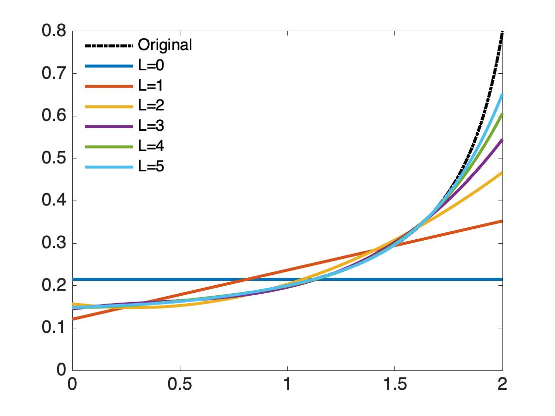
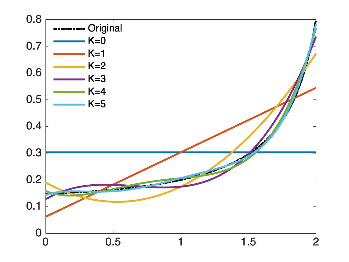
Figure 1: Plotted on the left are the original function $1/h_{1}$ on $[0,2]$ (marked as “Original”) and its optimal polynomial approximations ${\tilde{g}}_{L},0\leq L\leq 5$ (marked with different $L$), while on the right are the original function $1/h_{1}$ on $[0,2]$ and its Chebyshev polynomial approximations $g_{K},0\leq K\leq 5$ (marked with different $K$), where $h_{1}(t)=(9/4-t)(3+t)$ is the polynomial in (5.4), the underlying graph is the circulant graph ${\mathcal{C}}(1000,Q_{0})$ in (5.1) generated by $Q_{0}=\{1,2,5\}$ and the graph shift is the symmetric normalized Laplacian matrix on the circulant graph. The approximation errors $a_{L}$ in (4.10) to measure the approximation property between $\tilde{g}_{L},0\leq L\leq 5$ and $1/h_{1}$ are $0.4502$, $0.1852$, $0.0612$, $0.0212$, $0.0072$, $0.0025$ respectively, while approximation errors $b_{K}$ in (4.17) to measure the approximation property between $g_{K},0\leq K\leq 5$ and $1/h_{1}$ are $1.0463$, $0.5837$, $0.2924$, $0.1467$, $0.0728$, $0.0367$ respectively. This confirms the observation numerically that optimal/Chebyshev polynomials with higher degrees provide better approximations to the function $1/h_{1}$ either on the spectrum of normalized Laplacian on the circulant graph or on the interval $[0,2]$ containing the spectrum.

For $L\geq 0$, denote the set of all polynomials of degree at most $L$ by ${\mathcal{P}}_{L}$. In practice, we may not use the interpolation polynomial $g_{I}$ in (4.3), and hence the polynomial filter ${\bf G}=g_{I}({\bf S}_{1},\ldots,{\bf S}_{d})$ in the iterative approximation algorithm (3.5) and (3.6), as it is of high degree in general. By (3.7), the convergence rate of the iterative approximation algorithm (3.5) and (3.6) depends on the spectral radius in (4.1). Due to the above observation, we select ${\tilde{g}}_{L}\in{\mathcal{P}}_{L}$ such that

$${\tilde{g}}_{L}=\arg\!\min_{g\in{\mathcal{P}}_{L}}\sup_{\boldsymbol{\lambda}_{i}\in\Lambda}|1-g(\boldsymbol{\lambda}_{i})h(\boldsymbol{\lambda}_{i})|,$$ (4.4)

see Figure 1 for the approximation property of ${\tilde{g}}_{L},L\geq 0$ to the reciprocal $1/h_{1}$ of the polynomial $h_{1}(t)=(9/4-t)(3+t)$ in (5.4). For a multivariate polynomial $g\in{\mathcal{P}}_{L}$, we write

$$g({\bf t})=\sum_{|{\bf k}|\leq L}c_{\bf k}{\bf t}^{\bf k},$$

where $|{\bf k}|=k_{1}+\cdots+k_{d}$ and ${\bf t}^{\bf k}=t_{1}^{k_{1}}\cdots t_{d}^{k_{d}}$ for ${\bf t}=(t_{1},\ldots,t_{d})$ and ${\bf k}=(k_{1},\ldots,k_{d})$. Set ${\bf c}=(c_{\bf k})_{|{\bf k}|\leq L}$. Then for the case that all eigenvalues of ${\bf S}_{k},1\leq k\leq d$, are real, i.e., $\Lambda\subset{\mathbb{R}}^{d}$, the minimization problem (4.4) can be reformulated as a linear programming,

$$\min\ s\ \ {\rm subject\ to}\ -(s-1){\bf 1}\leq{\bf P}{\bf c}\leq(s+1){\bf 1},$$ (4.5)

where ${\bf P}=(h({\boldsymbol{\lambda}}_{i}){\boldsymbol{\lambda}}_{i}^{\bf k})_{1\leq i\leq N,|{\bf k}|\leq L}$, ${\bf 1}$ is the vector with all entries taking value 1, and we use standard componentwise ordering for real vectors.

Taking polynomial filters

$${\widetilde{\bf G}}_{L}={\tilde{g}}_{L}({\bf S}_{1},\ldots,{\bf S}_{d}),\ L\geq 0,$$ (4.6)

to approximate the inverse filter ${\bf H}^{-1}$, the iterative approximation algorithm (3.5) and (3.6) with the graph filter ${\bf G}$ replaced by ${\widetilde{\bf G}}_{L}$ becomes

$$\left\{\begin{array}[]{l}{\bf z}^{(m)}={\widetilde{\bf G}}_{L}{\bf e}^{(m-1)},\\ {\bf e}^{(m)}={\bf e}^{(m-1)}-{\bf H}{\bf z}^{(m)},\\ {\bf x}^{(m)}={\bf x}^{(m-1)}+{\bf z}^{(m)},\ m\geq 1,\end{array}\right.$$ (4.7)

with initials ${\bf e}^{(0)}$ and ${\bf x}^{(0)}$ given in (3.6). We call the above iterative algorithm (4.7) by the iterative optimal polynomial approximation algorithm, or IOPA in abbreviation.

Algorithm 4.1 The IOPA algorithm to implement the inverse filtering procedure ${\bf b}\longmapsto{\bf H}^{-1}{\bf b}$ at a vertex $i\in V$.

  Inputs: Polynomial coefficients of ${\bf H}$ and ${\widetilde{\bf G}}_{L}$, entries $S_{k}(i,j),j\in{\mathcal{N}}_{i}$ in the $i$-th row of the shift ${\bf S}_{k},1\leq k\leq d$, the value $b(i)$ of the input signal ${\bf b}=(b(i))_{i\in V}$ at the vertex $i$, and number $M$ of iteration.

  Initialization: Initial $e^{(0)}(i)=b(i)$, $x^{(0)}(i)=0$ and $n=0$.

  Iteration:     For $m=1,2,\ldots,M$       Step 1:  Use Algorithm 2.1 for $d=1$ and Algorithm 2.2 for $d\geq 2$ to implement the filtering procedure ${\bf e}^{(m-1)}\longmapsto{\bf z}^{(m)}={\widetilde{\bf G}}_{L}{\bf e}^{(m-1)}$ at the vertex $i$, and the output is the $i$-th entry $z^{(m)}(i)$ of the vector ${\bf z}^{(m)}$.       Step 2:  Use Algorithm 2.1 for $d=1$ and Algorithm 2.2 for $d\geq 2$ to implement the filtering procedure ${\bf z}^{(m)}\longmapsto{\bf w}^{(m)}={\bf H}{\bf z}^{(m)}$ at the vertex $i$, and the output is the $i$-th entries $w^{(m)}(i)$ of the vector ${\bf w}^{(m)}$.       Step 3: Update $i$-th entries of ${\bf e}^{(m)}$ and ${\bf x}^{(m)}$ by $e^{(m)}(i)=e^{(m-1)}(i)-{w}^{(m)}(i)$ and $x^{(m)}(i)=x^{(m-1)}(i)+z^{(m)}(i)$ respectively.     end

  Output: The approximated value $x(i)\approx x^{(M)}(i)$ is the output signal ${\bf H}^{-1}{\bf b}=(x(i))_{i\in V}$ at the vertex $i$.

Presented in Algorithm 4.1 is the implementation of IOPA algorithm at the vertex level in a distributed network. In each iteration of Algorithm 4.1, each vertex/agent of the distributed network needs about $O((L+1)^{d-1}+\prod_{k=1}^{d-1}(L_{k}+1))$ steps containing data exchanging among adjacent vertices and weighted sum of values at adjacent vertices in each iteration. The memory requirement for each vertex is about $O\big{(}(\deg{\mathcal{G}}+L_{k}+1)\prod_{k=1}^{d-1}(L_{k}+1)+(\det{\mathcal{G}})+L+1)(L+1)^{d-1})\big{)}$. The total operations of addition and multiplication in each iteration to implement the inverse filtering procedure ${\bf b}\longmapsto{\bf H}^{-1}{\bf b}$ via Algorithm 4.1 in a distributed network and procedure (4.7) in a central facility are almost the same, which are both about $O\big{(}N(\deg{\mathcal{G}}+1)(\prod_{k=1}^{d}(L_{k}+1)+(L+1)^{d})\big{)}$.

By (4.4), we have

$$\rho({\bf I}-{\widetilde{\bf G}}_{L}{\bf H})=\sup_{\boldsymbol{\lambda}_{i}\in\Lambda}|1-{\tilde{g}}_{L}(\boldsymbol{\lambda}_{i})h(\boldsymbol{\lambda}_{i})|$$ (4.8)

and $\rho({\bf I}-{\widetilde{\bf G}}_{L}{\bf H}),0\leq L\leq N-1$, is a nonnegative decreasing sequence with the last term $\rho({\bf I}-{\widetilde{\bf G}}_{N-1}{\bf H})$ being the same as $\rho({\bf I}-{\bf G}_{I}{\bf H})=0$ by (4.3), i.e.,

$$0=\rho({\bf I}-{\bf G}_{I}{\bf H})=\rho({\bf I}-{\widetilde{\bf G}}_{N-1}{\bf H})\leq\rho({\bf I}-{\widetilde{\bf G}}_{L+1}{\bf H})\leq\rho({\bf I}-{\widetilde{\bf G}}_{L}{\bf H})\leq\rho({\bf I}-{\widetilde{\bf G}}_{0}{\bf H}),\ 0\leq L\leq N-1.$$ (4.9)

This implies that the polynomial filters ${\bf G}_{L}$ with larger $L$ provide better approximation to the inverse filter ${\bf H}^{-1}$ and hence the corresponding IOPA algorithm (4.7) has faster convergence. In the following theorem, we show that the IOPA algorithm (4.7) converges exponentially when $L$ is appropriately chosen, see Subsection 5.1 for the numerical demonstration.

Theorem 4.2.

Let ${\bf S}_{1},...,{\bf S}_{d}$ be commutative graph shifts, ${\bf H}=h({\bf S}_{1},\ldots,{\bf S}_{d})$ be an invertible polynomial graph filter for some multivariate polynomial $h$, and let degree $L\geq 0$ be so chosen that

$$a_{L}:=\sup_{\boldsymbol{\lambda}_{i}\in\Lambda}|1-{\tilde{g}}_{L}(\boldsymbol{\lambda}_{i})h(\boldsymbol{\lambda}_{i})|<1.$$ (4.10)

Then for any graph signal $\bf b$, the sequence ${\bf x}^{(m)},m\geq 1$, in the IOPA algorithm (4.7) converges exponentially to ${\bf H}^{-1}{\bf b}$. Moreover, for any $r\in(a_{L},1)$, there exists a positive constant $C$ such that (3.7) holds.

Proof.

The conclusion follows from (4.8), (4.10) and Theorem 3.1 with ${\bf G}$ replaced by ${\widetilde{\mathbf{G}}}_{L}$. ∎

Let $L_{0}$ be the minimal nonnegative integer so that $a_{L_{0}}<1$. By (4.9) and Theorem 4.2, the inverse filtering procedure (3.1) can be implemented by applying the IOPA algorithm (4.7) with $L\geq L_{0}$ and the IOPA algorithm (4.7) converges faster when the higher degree $L$ of the optimal polynomial ${\tilde{g}}_{L}$ is selected, see Subsection 5.1 for the numerical demonstration. However, the implementation of IOPA algorithm (4.7) with larger $L$ at every agent/vertex in a distributed network has higher computational cost in each iteration and requires more memory for each agent/vertex, and also it takes higher computational cost to solve the the minimization problem (4.4) for larger $L$.

We finish this subsection with a remark on the IOPA algorithm (4.7) and the gradient descent method (3.13).

Remark 4.3.

For the case that the graph filter ${\bf H}$ has its spectrum contained in $[\alpha_{1},\alpha_{2}]$, the solution of the minimization problem (4.4) with $L=0$ is given by $\tilde{g}_{0}=2/(\alpha_{1}+\alpha_{2})$, where $\alpha_{1}=\min_{\boldsymbol{\lambda}_{i}\in\Lambda}h(\boldsymbol{\lambda}_{i})$ and $\alpha_{2}=\max_{\boldsymbol{\lambda}_{i}\in\Lambda}h(\boldsymbol{\lambda}_{i})$ are the minimal and maximal eigenvalues of ${\bf H}$ respectively. Therefore, to implement the inverse filtering procedure (3.1), the gradient descent method (3.13) with zero initial and optimal step length $\gamma=2/(\alpha_{1}+\alpha_{2})$ is the same as the proposed IOPA algorithm (4.7) with $L=0$, cf. Remark 3.2. By (4.9), we see that the IOPA algorithm with $L\geq 1$ has faster convergence than the gradient descent method does, at the cost of heavier computational cost at each iteration, see Table 1 and Figure 4 in Subsection 5.1 for numerical demonstrations.

4.2 Chebyshev polynomial approximation

In this subsection, we assume that commutative graph shifts ${\bf S}_{1},...,{\bf S}_{d}$ have their joint spectrum $\Lambda$ contained in the cubic $[{\boldsymbol{\mu}},{\boldsymbol{\nu}}]=[\mu_{1},\nu_{1}]\times\cdots\times[\mu_{d},\nu_{d}]$,

$${\boldsymbol{\lambda}}_{i}\in[{\boldsymbol{\mu}},{\boldsymbol{\nu}}]\ {\rm for\ all}\ {\boldsymbol{\lambda}}_{i}\in\Lambda,$$ (4.11)

and $h$ be a multivariate polynomial satisfying

$$h({\bf t})\neq 0\ \ {\rm for\ all}\ \ {\bf t}\in[{\boldsymbol{\mu}},{\boldsymbol{\nu}}].$$ (4.12)

Define Chebyshev polynomials $T_{k},k\geq 0$, by

$$T_{k}(s)=\left\{\begin{array}[]{lc}1&{\rm if}\hskip 2.84544ptk=0,\\ s&{\rm if}\hskip 2.84544ptk=1,\\ 2s{T}_{k-1}(s)-{T}_{k-2}(s)&{\rm if}\hskip 2.84544ptk\geq 2,\end{array}\right.$$

and shifted multivariate Chebyshev polynomials $\bar{T}_{\bf k},{\bf k}=(k_{1},\ldots,k_{d})\in{\mathbb{Z}}_{+}^{d}$, on $[{\boldsymbol{\mu}},{\boldsymbol{\nu}}]$ by

$$\bar{T}_{{\bf k}}({\bf t})=\prod_{i=1}^{d}T_{k_{i}}\Big{(}\frac{2t_{i}-\mu_{i}-\nu_{i}}{\nu_{i}-\mu_{i}}\Big{)},\ \ {\bf t}=(t_{1},...,t_{d})\in[{\boldsymbol{\mu}},{\boldsymbol{\nu}}].$$

By (4.12), $1/h$ is an analytic function on $[{\boldsymbol{\mu}},{\boldsymbol{\nu}}]$, and hence it has Fourier expansion in term of shifted Chebyshev polynomials $\bar{T}_{{\bf k}},{\bf k}\in{\mathbb{Z}}_{+}^{d}$,

$$\frac{1}{h({\bf t})}=\sum_{{\bf k}\in{\mathbb{Z}}_{+}^{d}}c_{{\bf k}}\bar{T}_{{\bf k}}({\bf t}),\ {\bf t}\in[{\boldsymbol{\mu}},{\boldsymbol{\nu}}],$$

where

$$c_{\bf k}=\frac{2^{d-p({\bf k})}}{\pi^{d}}\int_{[0,\pi]^{d}}\frac{\bar{T}_{\bf k}(t_{1}({\boldsymbol{\theta}}),\ldots,t_{d}({\boldsymbol{\theta}}))}{h(t_{1}({\boldsymbol{\theta}}),\ldots,t_{d}({\boldsymbol{\theta}}))}d\boldsymbol{\theta},\ {\bf k}\in{\mathbb{Z}}_{+}^{d},$$

$p({\bf k})$ is the number of zero components in ${\bf k}\in{\mathbb{Z}}^{d}_{+}$, and $t_{i}({\boldsymbol{\theta}})=\frac{\nu_{i}+\mu_{i}}{2}+\frac{\nu_{i}-\mu_{i}}{2}\cos(\theta_{i}),1\leq i\leq d,$ for $\boldsymbol{\theta}=(\theta_{1},...,\theta_{d})$. Define partial sum of the expansion (4.2) by

$$g_{K}({\bf t})=\sum_{|{\bf k}|\leq K}c_{{\bf k}}\bar{T}_{{\bf k}}({\bf t}),$$ (4.13)

where $|{\bf k}|=\sum_{i=1}^{d}k_{i}$ for ${\bf k}=(k_{1},...,k_{d})^{T}\in\mathbb{Z}_{+}^{d}$. Due to the analytic property of the polynomial $h$, the partial sum $g_{K},K\geq 0$, converges to $1/h$ exponentially [34],

$$b_{K}:=\sup_{{\bf t}\in[{\boldsymbol{\mu}},{\boldsymbol{\nu}}]}|1-h({\bf t})g_{K}({\bf t})|\leq Cr_{0}^{K},\ K\geq 0,$$ (4.14)

for some positive constants $C\in(0,\infty)$ and $r_{0}\in(0,1)$, see Figure 1 for the approximation property of $g_{K},K\geq 0$ to the reciprocal $1/h_{1}$ of the polynomial $h_{1}(t)=(9/4-t)(3+t)$ in (5.4).

Set

$${\bf G}_{K}=g_{K}({\bf S}_{1},\ldots,{\bf S}_{d}),\ K\geq 0,$$ (4.15)

and call the iterative approximation algorithm (3.5) and (3.6) with the graph filter ${\bf G}$ replaced by ${\bf G}_{K}$ by the iterative Chebyshev polynomial approximation algorithm, or ICPA in abbreviation,

$$\left\{\begin{array}[]{l}{\bf z}^{(m)}={\bf G}_{K}{\bf e}^{(m-1)},\\ {\bf e}^{(m)}={\bf e}^{(m-1)}-{\bf H}{\bf z}^{(m)},\\ {\bf x}^{(m)}={\bf x}^{(m-1)}+{\bf z}^{(m)},\ m\geq 1,\end{array}\right.$$ (4.16)

with initials ${\bf e}^{(0)}$ and ${\bf x}^{(0)}$ given in (3.6). In the following theorem, we show that the ICPA algorithm (4.16) converges exponentially, when the degree $K$ is so chosen that (4.17) holds, see Subsection 5.1 for the demonstration.

Theorem 4.4.

Let ${\bf S}_{1},...,{\bf S}_{d}$ be commutative graph shifts, ${\bf H}$ be a polynomial graph filter of the graph shifts, and let degree $K\geq 0$ of Chebyshev polynomial approximation be so chosen that

$$b_{K}:=\sup_{{\bf t}\in[{\boldsymbol{\mu}},{\boldsymbol{\nu}}]}|1-h({\bf t})g_{K}({\bf t})|<1.$$ (4.17)

Then for any graph signal $\bf b$, ${\bf x}^{(m)},m\geq 0$, in the ICPA algorithm (4.16) converges exponentially to ${\bf H}^{-1}{\bf b}$. Moreover for any $r\in(b_{K},1)$, there exists a positive constant $C$ such that

$$\|{\bf x}^{(m)}-{\bf H}^{-1}{\bf b}\|_{2}\leq C\|{\bf x}\|_{2}r^{m},\ m\geq 1.$$ (4.18)

Proof.

Following the argument used in (4.8), one may verify that

$$\rho({\bf I}-{\bf G}_{K}{\bf H})=\sup_{\boldsymbol{\lambda}_{i}\in\Lambda}|1-g_{K}(\boldsymbol{\lambda}_{i})h(\boldsymbol{\lambda}_{i})|\leq b_{K},$$ (4.19)

where the inequality holds by (4.11) and the definition (4.14) of $b_{K},K\geq 0$. Then the desired conclusion follows from (4.19) and Theorem 3.1 with ${\bf G}$ replaced by ${\mathbf{G}}_{K}$. ∎

Remark 4.5.

We remark that the convergence conclusion (4.18) in Theorem 4.4 can be improved as

$$\|{\bf x}^{(m)}-{\bf H}^{-1}{\bf b}\|_{2}\leq\frac{\|{\bf H}\|_{2}\|{\bf G}_{K}\|_{2}}{1-b_{K}}(b_{K})^{m}\|{\bf H}^{-1}{\bf b}\|_{2},\ m\geq 1.$$ (4.20)

provided that the commutative graph shifts ${\bf S}_{1},\ldots,{\bf S}_{d}$ are symmetric. Under the assumption that ${\bf S}_{1},\ldots,{\bf S}_{d}$ are symmetric, there exists a unitary matrix $\bf U$ such that they can be diagonalized simultaneously and hence ${\bf U}^{T}({\bf I}-{\bf H}{\bf G}_{K}){\bf U}$ is a diagonal matrix with diagonal entries $1-h({\boldsymbol{\lambda}}_{i})g_{K}({\boldsymbol{\lambda}}_{i}),1\leq i\leq N$, where ${\boldsymbol{\lambda}_{1}},\ldots,{\boldsymbol{\lambda}}_{N}\in\Lambda$. Therefore

$$\|{\bf I}-{\bf G}_{K}{\bf H}\|_{2}=\rho({\bf I}-{\bf G}_{K}{\bf H})=\sup_{1\leq i\leq N}|1-h({\boldsymbol{\lambda}}_{i})g_{K}({\boldsymbol{\lambda}}_{i})|\leq b_{K}$$ (4.21)

where the last inequality follows from (4.11) and (4.14). The desired exponential convergence can be obtained by applying the similar argument used in Theorem 3.1 with (3.2) and (3.3) replaced by (4.17) and (4.21).

Remark 4.6.

We remark that each iteration in the ICPA algorithm (4.16) can be implemented at vertex level, see Algorithm 4.2.

Algorithm 4.2 The ICPA algorithm to implement the inverse filtering procedure ${\bf b}\longmapsto{\bf H}^{-1}{\bf b}$ at a vertex $i\in V$.

  Inputs: Polynomial coefficients of polynomial filters ${\bf H}$ and ${\bf G}_{K}$, entries $S_{k}(i,j),j\in{\mathcal{N}}_{i}$ in the $i$-th row of the shifts ${\bf S}_{k},1\leq k\leq d$, the value $b(i)$ of the input signal ${\bf b}=(b(i))_{i\in V}$ at the vertex $i$, and number $M$ of iteration.

  Initialization: Initial $e^{(0)}(i)=b(i)$, $x^{(0)}(i)=0$ and $n=0$.

  Iteration: Use the iteration in Algorithm 4.1 except replacing ${\widetilde{\bf G}}_{L}$ by ${\bf G}_{K}$ in (4.15), and the output is $x^{(M)}(i)$.

  Output: The approximated value $x(i)\approx x^{(M)}(i)$ is the output signal ${\bf H}^{-1}{\bf b}=(x(i))_{i\in V}$ at the vertex $i$.

In each iteration of the ICPA algorithm (4.16), every agent in a distributed network (vertex of the graph) needs about $O((K+1)^{d-1}+\prod_{k=1}^{d-1}(L_{k}+1))$ steps with each step containing data exchanging among adjacent vertices and weighted linear combination of values at adjacent vertices. The memory requirement for each agent is about $O\big{(}(\deg{\mathcal{G}}+L_{d}+1)\prod_{k=1}^{d-1}(L_{k}+1)+(\deg{\mathcal{G}}+K+1)(K+1)^{d-1}\big{)}$. The total operations of addition and multiplication to implement each iteration of Algorithm 4.2 in a distributed network and to implement (4.16) in a central facility are almost the same, which are both about $O\big{(}N(\deg{\mathcal{G}}+1)(\prod_{k=1}^{d}(L_{k}+1)+(K+1)^{d})\big{)}$.

Remark 4.7.

By (4.14), an inverse filtering procedure (3.1) can be approximately implemented by the filter procedure ${\bf G}_{K}{\bf x}$ with large $K$, i.e., ${\bf H}^{-1}{\bf x}\approx{\bf G}_{K}{\bf x}$ for large $K$. The above implementation of the inverse filtering has been discussed in [6, 46] for the case that ${\bf H}$ is a polynomial graph filter of one shift, and it is known as the Chebyshev polynomial approximation algorithm (CPA). We remark that in the single graph shift setting, the approximation ${\bf G}_{K}{\bf x}$ in the CPA is the same as the first term ${\bf x}^{(1)}$ in the ICPA algorithm (4.16). To implement the inverse filtering with high accuracy, the CPA requires Chebyshev polynomial approximation of high degree, which means more integrals involved in coefficient calculations. On the other hand, we can select Chebyshev polynomial approximation of lower degree in the ICPA algorithm (4.16) to reach the same accuracy with few iterations. By Theorem 4.4, the ICPA algorithm (4.16) has exponential convergent rate $b_{K}$, which has limit zero as $K\to\infty$. This indicates that the ICPA algorithm converges faster for large $K$, however for each agent in a distributed network, its data processing system need more memory to store data and time to process data, and its communication system costs more for larger $K$ too. Our simulation in the next section confirms the above observation, see Table 1 and Figure 4 in Subsection 5.1.

5 Numerical simulations

In this section, we demonstrate the iterative optimal polynomial approximation (IOPA) algorithm (4.7) and the iterative Chebyshev polynomial approximation (ICPA) algorithm (4.16) to implement an inverse filtering procedure, and compare their performances with the gradient descent method (3.13) with zero initial [41], and the autoregressive moving average (ARMA) algorithm (3.16) and (3.17) [19].

Let $N\geq 1$ and $Q=\{q_{1},\ldots,q_{M}\}$ be a set of integers ordered so that $1\leq q_{1}<\ldots<q_{M}<N/2$. The circulant graph ${\mathcal{C}}(N,Q)$ generated by $Q$ has the vertex set $V_{N}=\{0,1,\ldots,N-1\}$ and the edge set

$$E_{N}(Q)=\{(i,i\pm q\ {\rm mod}\ N),\ i\in V_{N},q\in Q\},$$ (5.1)

where $a=b\ {\rm mod}\ N$ if $(a-b)/N$ is an integer. Shown in Figure 2 is a circulant graph with $N=50$ and $Q=\{1,2,5\}$. Circulant graphs are widely used in image processing [10, 11, 23, 24, 48]. In Subsection 5.1, we demonstrate the performance of the proposed IOPA and ICPA algorithms on the implementation of the inverse filtering on circulant graphs.

Graph signal denoising is one of the most popular applications in graph filtering [7, 9, 13, 19, 21, 37, 40, 49, 50]. and in some cases, it can be recasted as an inverse filtering procedure. In Subsection 5.2, we consider denoising noisy sampling data

$${\bf b}_{i}={\bf x}(t_{i})+\boldsymbol{\eta}_{i},\ 1\leq i\leq M,$$ (5.2)

of some time-varying graph signal ${\bf x}(t)$ on random geometric graphs, which is governed by a differential equation

$${\bf x}^{\prime\prime}(t)={\bf P}{\bf x}(t),$$ (5.3)

where ${\boldsymbol{\eta}}_{i},1\leq i\leq M$, are noises with noise level $\eta=\max_{1\leq i\leq M}\|{\boldsymbol{\eta}}_{i}\|_{\infty}$, the sampling procedure is taken uniformly at $t_{i}=t_{1}+(i-1)\delta,1\leq i\leq M$, with uniform sampling gap $\delta>0$, and ${\bf P}$ is a graph filter with small geodesic-width.

Finally in Subsection 5.3, we apply the proposed IOPA and ICPA algorithms to denoise the hourly temperature dataset collected at $218$ locations in the United States.

5.1 Iterative approximation algorithms on circulant graphs

Table 1: Average relative iteration error over 1000 trials for the ARMA method, GD0 algorithm, and IOPA and ICPA algorithms with different degrees to implement the inverse filtering ${\bf b}\longmapsto{\bf H}_{1}^{-1}{\bf b}$ on the circulant graph ${\mathcal{C}}(1000,Q_{0})$.

	1	2	3	4	5	7	9	11	14	17	20
ARMA	.3259	.2583	.1423	.1098	.0718	.0381	.0207	.0113	.0047	.0019	.0008
GD0	.2350	.0856	.0349	.0147	.0063	.0012	.0002	.0000	.0000	.0000	.0000
ICPA0	.5686	.4318	.3752	.3521	.3441	.3460	.3577	.3743	.4061	.4451	.4913
ICPA1	.4494	.2191	.1103	.0566	.0295	.0082	.0024	.0007	.0001	.0000	.0000
ICPA2	.1860	.0412	.0098	.0024	.0006	.0000	.0000	.0000	.0000	.0000	.0000
IOPA1	.1545	.0266	.0047	.0008	.0002	.0000	.0000	.0000	.0000	.0000	.0000
ICPA3	.0979	.0113	.0014	.0002	.0000	.0000	.0000	.0000	.0000	.0000	.0000
ICPA4	.0499	.0030	.0002	.0000	.0000	.0000	.0000	.0000	.0000	.0000	.0000
IOPA2	.0365	.0019	.0001	.0000	.0000	.0000	.0000	.0000	.0000	.0000	.0000
ICPA5	.0225	.0007	.0000	.0000	.0000	.0000	.0000	.0000	.0000	.0000	.0000
IOPA3	.0167	.0003	.0000	.0000	.0000	.0000	.0000	.0000	.0000	.0000	.0000
IOPA4	.0044	.0000	.0000	.0000	.0000	.0000	.0000	.0000	.0000	.0000	.0000
IOPA5	.0019	.0000	.0000	.0000	.0000	.0000	.0000	.0000	.0000	.0000	.0000

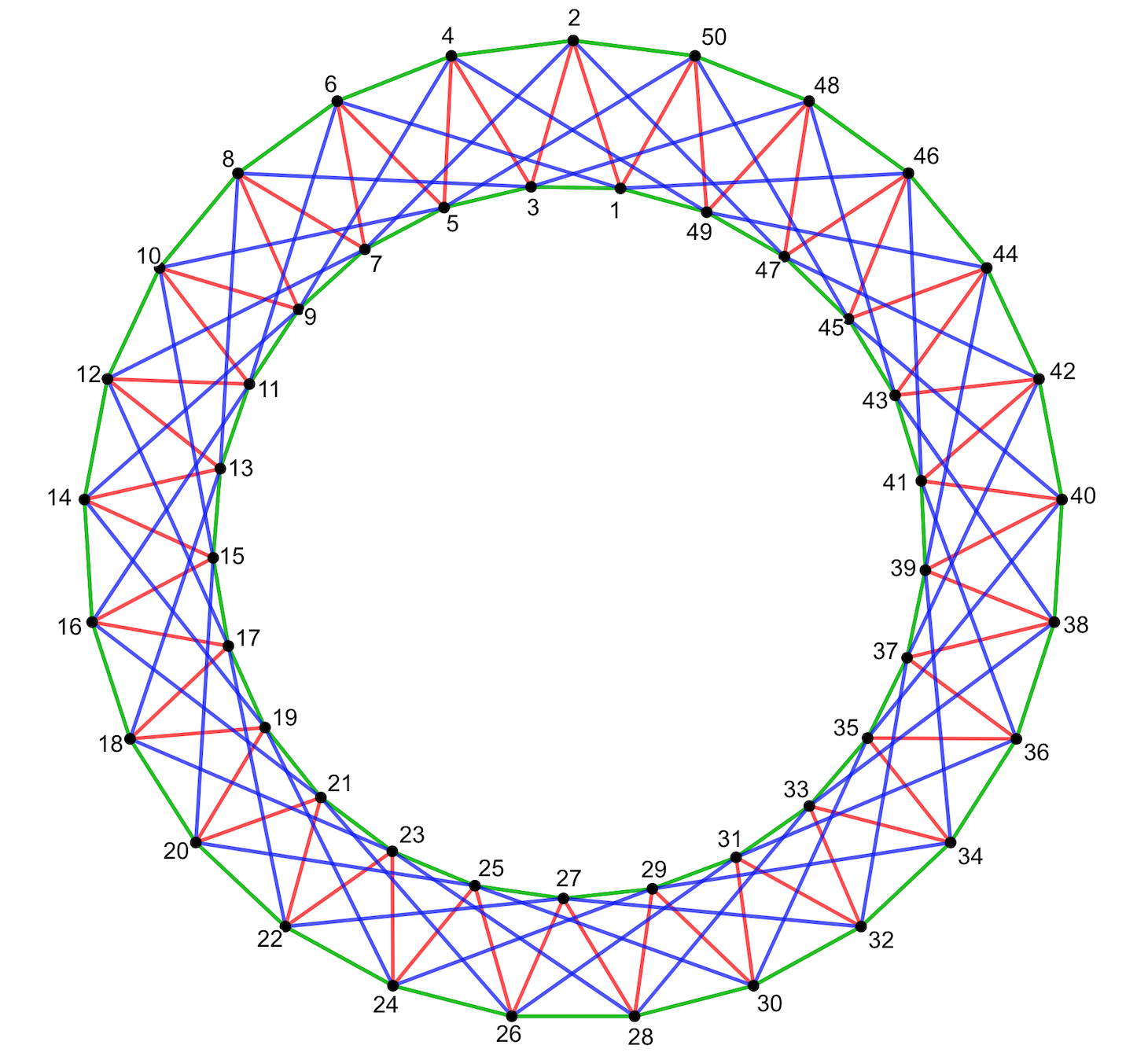
Figure 2: The circulant graph with 50 nodes and generating set $Q_{0}=\{1,2,5\}$, where edges in red/green/blue are also edges of the circulant graphs $\mathcal{C}_{1}$, $\mathcal{C}_{2}$ and $\mathcal{C}_{5}$ generated by $\{1\},\{2\},\{5\}$ respectively.

In this section, we consider the circulant graph ${\mathcal{C}}(N,Q_{0})$ generated by $Q_{0}=\{1,2,5\}$, the input graph signal ${\bf x}$ with entries randomly selected in the interval $[-1,1]$, and the graph signal ${\bf b}={\bf H}_{1}{\bf x}$ as the observation, where

$$h_{1}(t)=(9/4-t)(3+t)$$ (5.4)

and

$${\bf H}_{1}=h_{1}({\mathbf{L}}^{\rm sym}_{{\mathcal{C}}(N,Q_{0})})$$

is a polynomial graph filter of the symmetric normalized Laplacian ${\bf L}^{\rm sym}_{{\mathcal{C}}(N,Q_{0})}$ on ${\mathcal{C}}(N,Q_{0})$, see Remark A.1 for commutative graph shifts on circulant graphs. We implement the inverse filtering ${\bf b}\longmapsto{\bf H}_{1}^{-1}{\bf b}$ through the IOPA algorithm (4.7) and ICPA algorithm (4.16) on the circulant graph ${\mathcal{C}}(N,Q_{0})$. By Theorems 4.2 and 4.4, the IOPA algorithm with $L\geq 0$ and the ICPA algorithm with $K\geq 1$ converge, and we denote those algorithms by IOPA$L$ and ICPA$K$ for abbreviation. Notice that the filter ${\bf H}_{1}$ is positive definite, and

$$\frac{1}{h_{1}(t)}=\frac{4/21}{9/4-t}+\frac{4/21}{3+t}\vspace{-.4em}$$

meets the requirement (3.15) for the ARMA. For the circulant graph $\mathcal{C}(N,Q_{0})$ with $N=1000$, we also implement the inverse filtering ${\bf b}\longmapsto{\bf H}_{1}^{-1}{\bf b}$ by the gradient descent method with zero initial, GD0 in abbreviation, with the optimal step length $\gamma=2/(6.7500+2.5588)$, and the ARMA method, where $2.5588$ and $6.7500$ are the minimal and maximal eigenvalues for ${\bf H}_{1}$ respectively.

Set the relative iteration error

$$E(m,{\bf x})={\|{\bf x}^{(m)}-{\bf x}\|_{2}}/{\|{\bf x}\|_{2}},\ m\geq 1,$$

where ${\bf x}^{(m)},m\geq 1$, are the output at $m$-th iteration. Shown in Table 1 are the comparisons of the ARMA algorithm, the GD$0$ algorithm, and IOPA$L$ and ICPA$K$ algorithms regard to the average of the relative iteration error for implementing the inverse filtering on the circulant graph ${\mathcal{C}}(1000,Q_{0})$ over 1000 trials, where $0\leq L,K\leq 5$. This confirms that exponential convergence and applicability of the inverse filtering procedure ${\bf b}\longmapsto{\bf H}_{1}^{-1}{\bf b}$ of IOPA$L$, $0\leq L\leq 5$ and ICPA$K$, $1\leq K\leq 5$ on the circulant graph ${\mathcal{C}}(1000,Q_{0})$. The average exponential convergence rates of IOPA$L$, $0\leq L\leq 5$, over 1000 trials are $0.4401,0.1820,0.0593,0.0208,0.0067,0.0023$ respectively, and the average exponential convergence rates of ICPA$K$, $1\leq K\leq 5$, are $0.5485$, $0.2804$, $0.1459$, $0.0685$, $0.0334$ respectively. It is observed that average exponential convergence rates of IOPA$L$, $0\leq L\leq 5$ and ICPA$K$, $1\leq K\leq 5$, are close to their theoretical bounds $a_{L},0\leq L\leq 5$ in (4.10) and $b_{K},1\leq K\leq 5$ in (4.17) respectively, which are listed in the caption of Figure 1. By the third row in Table 1, we see that the ICPA0 does not yield the desired inverse filtering result. The reason for the divergence is that the theoretical bound $b_{0}=1.0463$ in (4.17) is strictly larger than one. From Table 1, we observe that the IOPA$L$ algorithms with higher degree $L$ (resp. the ICPA$K$ with higher degree $K$) have faster convergence, and the IOPA$L$ algorithm outperforms the ICPA$K$ algorithm when the same degree $L=K$ is selected. Comparing with the ARMA algorithm and the GD0 algorithm, we observe that the proposed IOPA$L$ algorithms with $L\geq 1$ and ICPA$K$ algorithms with $K\geq 2$ have faster convergence, while the GD$0$=IOPA$0$ algorithm outperforms the ICPA$K$ when $K=1$ and the ARMA has slowest convergence.

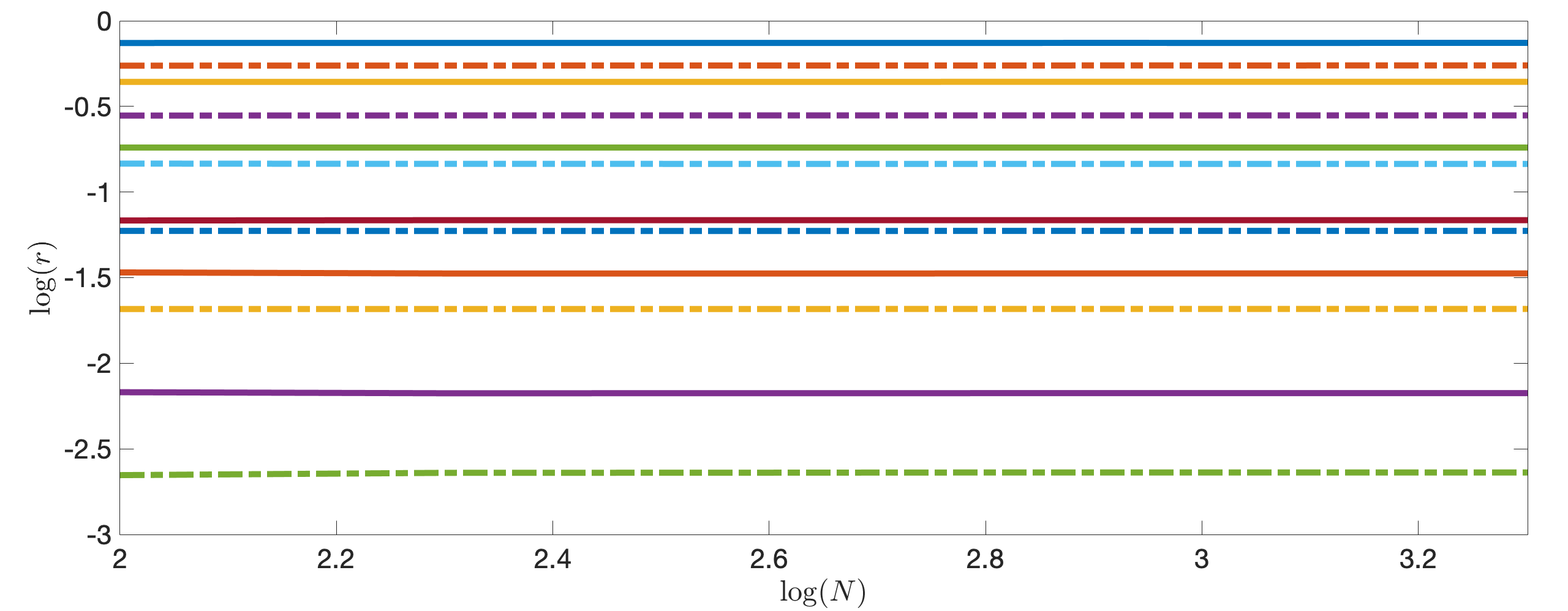
Figure 3: Plotted from top to bottom are the average exponential convergence rate $r$ in the logarithmic scale over 1000 trials by ARMA, ICPA1, GD0, ICPA2, IOPA1, ICPA3, ICPA4, IOPA2, ICPA5, IOPA3, IOPA4, IOPA5 to implement the inverse filtering ${\bf b}\longmapsto{\bf H}_{1}^{-1}{\bf b}$ on circulant graphs ${\mathcal{C}}(N,Q_{0})$ with $100\leq N\leq 2000$, respectively.

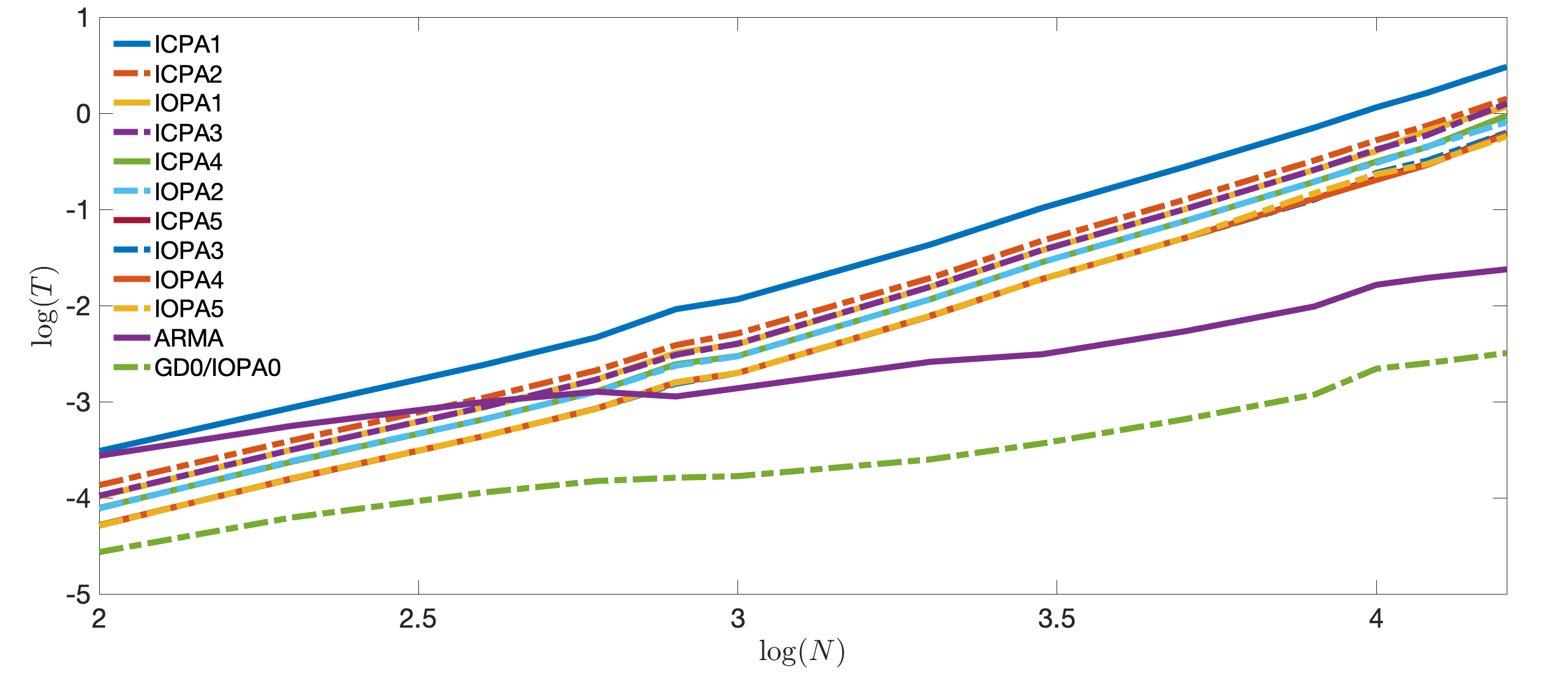
Figure 4: Plotted are the average of total running time $T$ in the logarithmic scale for the GD0, ARMA and the IOPA$L$ and ICPA$K$ algorithms with $1\leq L,K\leq 5$ to implement the inverse filtering on circulant graphs ${\mathcal{C}}(N,Q_{0})$ with $100\leq N\leq 16000$.

We also apply ARMA, GD0, and IOPA$L$ and ICPA$K$ with $1\leq L,K\leq 5$ to implement inverse filtering procedure associated with ${\bf H}_{1}=h_{1}({\mathbf{L}}^{\rm sym}_{{\mathcal{C}}(N,Q_{0})})$ on the circulant graph ${\mathcal{C}}(N,Q_{0})$ with $h_{1}$ in (5.4) and $N\geq 100$. All experiments were performed on MATLAB R2017b, running on a DELL T7910 workstation with two Intel Core E5-2630 v4 CPUs (2.20 GHz) and 32GB memory. From the simulations, we observe that the exponential convergence rate $r$ for the proposed algorithms is almost independent on $N\geq 100$, see Figure 3, and the number of iterations to ensure the relative iteration error $E(m,{\bf x})\leq 10^{-3}$ are $20,8,11,5,4,4,3,3,2,2,2,2$ for ARMA, GD0, ICPA1, ICPA2, IOPA1, ICPA3, ICPA4, IOPA2, ICPA5, IOPA3, IOPA4, IOPA5 respectively. Shown in Figure 4 is the average running time $T$ in the logarithmic scale over 1000 trials, where the running time $T$ is measured in seconds to ensure the relative iteration error $E(m,{\bf x})\leq 10^{-3}$. From our simulations, we see that there is a complicated trade-off between the convergence rate and the running time to apply our proposed algorithms, ARMA and GD0 for the implementation of an inverse filtering procedure.

5.2 Denoising time-varying signals

In this section, we consider denoising noisy sampling data of some time-varying graph signal ${\bf x}(t)$ on random geometric graphs, which is governed by the differential equation (5.3). Discretizing the differential equation (5.3) gives

$$\delta^{-2}\big{(}{\bf x}(t_{i+1})+{\bf x}(t_{i-1})-2{\bf x}(t_{i})\big{)}\approx{\bf P}{\bf x}(t_{i}),$$ (5.5)

where $i=1,\ldots,M$. Applying the trivial extension ${\bf x}(t_{0})={\bf x}(t_{1})$ and ${\bf x}(t_{M+1})={\bf x}(t_{M})$ around the boundary, we can reformulate (5.5) in a recurrence relation,

$${\bf x}(t_{i})\approx(2{\bf I}+\delta^{2}{\bf P}){\bf x}(t_{i-1})-{\bf x}(t_{i-2}),2\leq i\leq M,$$ (5.6)

with ${\bf x}(t_{0})={\bf x}(t_{1})$. Let ${\mathcal{T}}=(T,F)$ be the line graph with the vertex set $T=\{t_{1},\cdots,t_{M}\}$ and edge set $F=\{(t_{1},t_{2}),\ldots,(t_{M-1},t_{M})\}\cup\{(t_{M},t_{M-1}),\ldots,(t_{2},t_{1})\}$. Denote Kronecker product of two matrices ${\bf A}$ and ${\bf B}$ by ${\bf A}\otimes{\bf B}$, and the Laplacian matrix of the line graph ${\mathcal{T}}$ with vertices $\{t_{1},\ldots,t_{M}\}$ by ${\bf L}_{\mathcal{T}}$. Then we can reformulate the recurrence relation (5.6) in the matrix form

$$(\delta^{-2}{\bf L}_{\mathcal{T}}\otimes{\bf I}+{\bf I}\otimes{\bf P}){\bf X}\approx{\bf 0},$$ (5.7)

where ${\bf X}$ is the vectorization of discrete time signals ${\bf x}(t_{1}),\ldots,{\bf x}(t_{M})$. In most of applications [10, 14, 28, 49], the time-varying signal ${\bf x}(t)$ at every moment $t$ has certain smoothness in the vertex domain, which is usually described by

$$({\bf x}(t_{i}))^{T}{\bf L}_{\mathcal{G}}^{\rm sym}{\bf x}(t_{i})\approx 0,\ 1\leq i\leq M,$$ (5.8)

where ${\bf L}_{\mathcal{G}}^{\rm sym}$ is the symmetric normalized Laplacian on the connected, undirected and unweighted graph ${\mathcal{G}}=(V,E)$. Based on the observations (5.7) and (5.8), we propose the following Tikhonov regularization approach

$$\widehat{\bf X}:={\rm arg}\min_{\bf Y}\|{\bf Y}-{{\bf B}}\|_{2}^{2}+\alpha{\bf Y}^{T}({\bf I}\otimes{{\bf L}^{\rm sym}_{\mathcal{G}}}){\bf Y}+\beta{\bf Y}^{T}(\delta^{-2}{\bf L}_{\mathcal{T}}\otimes{\bf I}+{\bf I}\otimes{\bf P}){\bf Y},$$ (5.9)

where ${\bf B}$ is the vectorization of the observed noisy data ${\bf b}_{1},\ldots,{\bf b}_{M}$, and $\alpha,\beta$ are penalty constants in the vertex and “temporal” domains to be appropriately chosen [26].

Set

$${\bf D}_{\alpha,\beta}={\bf I}+\alpha{\bf I}\otimes{{\bf L}^{\rm sym}_{\mathcal{G}}}+\beta(\delta^{-2}{\bf L}_{\mathcal{T}}\otimes{\bf I}+{\bf I}\otimes{\bf P}),\ \alpha,\beta\geq 0.$$

The minimization problem (5.9) has an explicit solution

$$\widehat{\bf X}=({\bf D}_{\alpha,\beta})^{-1}{\bf B},$$ (5.10)

when ${\bf I}+\alpha{\bf L}^{\rm sym}_{\mathcal{G}}+\beta{\bf P}$ is positive definite. Set ${\bf S}_{1}={\bf I}\otimes{{\bf L}^{\rm sym}_{\mathcal{G}}}$ and ${\bf S}_{2}=\frac{1}{2}{\bf L}_{\mathcal{T}}\otimes{\bf I}$. As shown in Proposition A.2 of Appendix A.2, ${\bf S}_{1}$ and ${\bf S}_{2}$ are commutative graph shifts on the Cartesian product graph ${\mathcal{T}}\times{\mathcal{G}}$. Moreover one may obtain from (A.3) and (A.5) that ${\bf S}_{1}$ and ${\bf S}_{2}$ have their joint spectrum contained in $[0,2]^{2}$. Therefore for the case that ${\bf P}=p({\bf L}^{\rm sym}_{\mathcal{G}})$ for some polynomial $p$, ${\bf D}_{\alpha,\beta}=h_{\alpha,\beta}({\bf S}_{1},{\bf S}_{2})$ is a polynomial graph filter of commutative graph filters ${\bf S}_{1}$ and ${\mathbf{S}}_{2}$, where $h_{\alpha,\beta}(t_{1},t_{2})=1+\alpha t_{1}+\beta p(t_{1})+2\beta\delta^{-2}t_{2}$. Moreover, one may verify that ${\bf D}_{\alpha,\beta}$ is positive definite if

$$h_{\alpha,\beta}(t_{1},t_{2})>0,\ \ 0\leq t_{1},t_{2}\leq 2,$$

which is satisfied if $1+\beta p(t_{1})>0$ for all $0\leq t_{1}\leq 2$. Hence we may use the IOPA algorithm (4.7) and the ICPA algorithm (4.16) with the polynomial filter ${\bf H}$ being replaced by ${\bf D}_{\alpha,\beta}$ to implement the denoising procedure (5.10). By the exponential convergence of the proposed algorithms, we may use their outputs at $m$-th iteration with large $m$ as denoised time-varying signals.

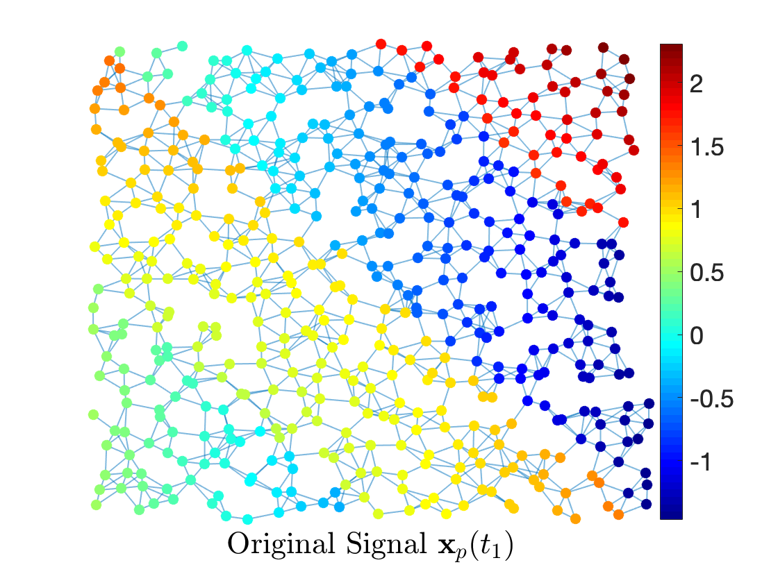
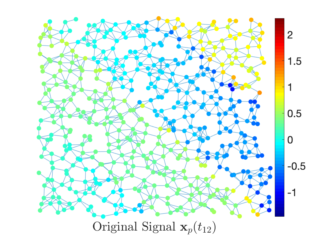
Figure 5: Presented on the left and right are the first snapshot ${\bf x}_{p}(t_{1})$ and the middle snapshot ${\bf x}_{p}(t_{12})$ of a time-varying signal ${\bf x}_{p}(t_{m}),1\leq m\leq 24$, on the random geometric graph ${\mathcal{G}}_{512}$ respectively. The qualities $({\bf x}_{p}(t_{m}))^{T}{\bf L}_{{\mathcal{G}}_{512}}^{\rm sym}{\bf x}_{p}(t_{m})$ to measure smoothness of ${\bf x}_{p}(t_{m})$ in the vertex domain are $84.1992$ and $42.4746$ for $m=1,12$ respectively, which indicates that the graph signal ${\bf x}(t_{12})$ in the last snapshot is smoother than the initial graph signal ${\bf x}(t_{1})$.

Let ${\mathcal{G}}_{512}$ be the random geometric graph reproduced by the GSPToolbox, which has 512 vertices randomly deployed in the region $[0,1]^{2}$ and an edge existing between two vertices if their physical distance is not larger than $\sqrt{2/512}=1/16$ [21, 31]. Denote the symmetric normalized Laplacian matrix on ${\mathcal{G}}_{512}$ by ${\bf L}^{\rm sym}_{{\mathcal{G}}_{512}}$ and the coordinates of a vertex $i$ in ${\mathcal{G}}_{512}$ by $(i_{x},i_{y})$. For the simulations in this section, the time-varying signal ${\bf x}(t_{m}),1\leq m\leq M$, is given in (5.5), where $M=24,\delta=0.1$, the governing filter is given by ${\bf P}=-{\bf I}+{\bf L}^{\rm sym}_{{\mathcal{G}}_{512}}/2$, and the initial graph signal ${\bf x}_{p}(t_{1})$ is a blockwise polynomial consisting of four strips and imposing $(0.5-2i_{x})$ on the first and third diagonal strips and $(0.5+i_{x}^{2}+i_{y}^{2})$ on the second and fourth strips respectively [21]. Shown in Figure 5 are two snapshots of the above time-varying graph signal.

Appropriate selection of the penalty constants $\alpha,\beta$ in the vertex and temporal domains is crucial to have a satisfactory denoising performance. In the simulations, we let noise entries of $\boldsymbol{\eta}_{i},1\leq i\leq 24$ in (5.3), be i.i.d. variables uniformly selected in the range $[-\eta,\eta]$, and we take

$$\alpha=\frac{{\mathbb{E}}\|{\bf B}-{\bf X}\|_{2}^{2}}{{\mathbb{E}}\big{(}{\bf B}^{T}({\bf I}\otimes{\bf L}^{\rm sym}_{{\mathcal{G}}_{512}}){\bf B}\big{)}}=\frac{MN\eta^{2}/3}{{\bf X}^{T}({\bf I}\otimes{\bf L}^{\rm sym}_{{\mathcal{G}}_{512}}){\bf X}+MN\eta^{2}/3}\approx\frac{\eta^{2}}{0.2306+\eta^{2}},$$ (5.11)

and

$$\beta \hskip-9.39545pt= \hskip-9.39545pt\frac{{\mathbb{E}}\|{\bf B}-{\bf X}\|_{2}^{2}}{2{\mathbb{E}}\big{(}{\bf B}^{T}(\delta^{-2}{\bf L}_{\mathcal{T}}\otimes{\bf I}+{\bf I}\otimes{\bf P}){\bf B}\big{)}}\approx 0.0026$$ (5.12)

to balance the fidelity term and the regularization terms on the vertex and temporal domains in the Tikhonov regularization approach (5.9).

We use the IOPA algorithm (4.7) with $L=1$, the ICPA algorithm (4.16) with $K=1$ and the gradient descent method (3.13) with zero initial to implement the inverse filter procedure ${\bf B}\longmapsto\widehat{\bf X}={\bf D}_{\alpha,\beta}^{-1}{\bf B}$, denoted by IOPA1$(\alpha,\beta)$, ICPA1$(\alpha,\beta)$ and GD0$(\alpha,\beta)$ respectively. Let $\widehat{\bf X}^{(m)},m\geq 1$, be the outputs of either the IOPA1$(\alpha,\beta)$ algorithm, or the ICPA1$(\alpha,\beta)$ algorithm, or the GD0$(\alpha,\beta)$ method at $m$-th iteration. To measure the denoising performance of our approaches, we define the input signal-to-noise ratio

$${\rm ISNR}=-20\log_{10}{\|{\bf B}-{\bf X}\|_{2}}/{\|{\bf X}\|_{2}},$$

and the output signal-to-noise ratio

$${\rm SNR}(m)=-20\log_{10}{\|\widehat{\bf X}^{(m)}-{\bf X}\|_{2}}/{\|{\bf X}\|_{2}},\ m\geq 1,$$

and

$${\rm SNR}(\infty)=-20\log_{10}{\|\widehat{\bf X}-{\bf X}\|_{2}}/{\|{\bf X}\|_{2}}.$$

Table 2: The average of the signal-to-noise ratio ${\rm SNR}(m),m=1,2,4,6,\infty$ for the noise level $\eta=3/4,1/2,1/4,1/8$ over 1000 trials, where penalty constants $\alpha$ and $\beta$ are given in (5.11) and (5.12) respectively.

m	1	2	4	6	$\infty$
$\eta$=3/4, ISNR= 3.3755
IOPA1($\alpha$, 0)	6.5777	6.8047	6.7927	6.7926	6.7926
IOPA1(0, $\beta$)	6.0597	6.0907	6.0735	6.0735	6.0735
IOPA1($\alpha$, $\beta$)	7.4797	8.5330	8.4942	8.4931	8.4930
ICPA1($\alpha$, 0)	6.4581	6.8169	6.7928	6.7926	6.7926
ICPA1(0, $\beta$)	6.0433	6.0899	6.0735	6.0735	6.0735
ICPA1($\alpha$, $\beta$)	7.4036	8.4602	8.4924	8.4930	8.4930
GD0($\alpha$, 0)	4.9399	6.7283	6.8062	6.7943	6.7926
GD0(0, $\beta$)	5.0027	6.3873	6.1225	6.0787	6.0735
GD0($\alpha$, $\beta$)	4.1778	6.9998	8.3432	8.4750	8.4930
$\eta$=1/2, ISNR=6.8975
IOPA1($\alpha$, 0)	9.2211	9.3576	9.3544	9.3544	9.3544
IOPA1(0, $\beta$)	9.4981	9.6116	9.5949	9.5949	9.5949
IOPA1($\alpha$, $\beta$)	10.0425	11.0678	11.0624	11.0620	11.0620
ICPA1($\alpha$, 0)	9.1525	9.3617	9.3544	9.3544	9.3544
ICPA1(0, $\beta$)	9.5037	9.6110	9.5949	9.5949	9.5949
ICPA1($\alpha$, $\beta$)	9.7218	11.0092	11.0613	11.0620	11.0620
GD0($\alpha$, 0)	7.1610	9.2163	9.3568	9.3546	9.3544
GD0(0, $\beta$)	6.8746	9.5953	9.6392	9.6000	9.5949
GD0($\alpha$, $\beta$)	5.3263	8.9866	10.8804	11.0423	11.0620
$\eta$=1/4, ISNR= 12.9164
IOPA1($\alpha$, 0)	13.8837	13.9053	13.9053	13.9053	13.9053
IOPA1(0, $\beta$)	15.0923	15.6251	15.6109	15.6108	15.6108
IOPA1($\alpha$, $\beta$)	14.6334	15.9121	15.9192	15.9192	15.9192
ICPA1($\alpha$, 0)	13.8693	13.9055	13.9053	13.9053	13.9053
ICPA1(0, $\beta$)	15.2045	15.6255	15.6109	15.6108	15.6108
ICPA1($\alpha$, $\beta$)	14.1329	15.8756	15.9190	15.9192	15.9192
GD0($\alpha$, 0)	12.2195	13.8694	13.9052	13.9053	13.9053
GD0(0, $\beta$)	8.5703	14.2275	15.6302	15.6153	15.6108
GD0($\alpha$, $\beta$)	7.2800	12.7687	15.7309	15.9044	15.9192
$\eta$=1/8, ISNR= 18.9370
IOPA1($\alpha$, 0)	19.2287	19.2299	19.2299	19.2299	19.2299
IOPA1(0, $\beta$)	19.7355	21.6233	21.6187	21.6187	21.6187
IOPA1($\alpha$, $\beta$)	19.1231	21.6012	21.6335	21.6336	21.6336
ICPA1($\alpha$, 0)	19.2275	19.2299	19.2299	19.2299	19.2299
ICPA1(0, $\beta$)	20.1427	21.6275	21.6187	21.6187	21.6187
ICPA1($\alpha$, $\beta$)	18.9606	21.5903	21.6335	21.6336	21.6336
GD0($\alpha$, 0)	18.5134	19.2279	19.2299	19.2299	19.2299
GD0(0, $\beta$)	9.1228	17.0384	21.5398	21.6206	21.6187
GD0($\alpha$, $\beta$)	8.6071	16.0831	21.3347	21.6140	21.6336

Presented in Table 2 are the average over 1000 trials of ${\rm ISNR}$ and ${\rm SNR}(m),m=1,2,4,6,\infty$. From Table 2, we observe that the denoising procedure ${\bf B}\longmapsto\widehat{\bf X}={\bf D}_{\alpha,\beta}^{-1}{\bf B}$ via Tikhonov regularization (5.9) on the temporal-vertex domain can improve the signal-to-noise ratio in the range from 2dBs to 5dBs, depending on the noise level $\eta$. Also we see that the denoising procedure ${\bf B}\longmapsto\widehat{\bf X}^{(m)}$ via the output of the $m$-th iteration in IOPA1($\alpha,\beta$) algorithm with $m\geq 2$, the GD0$(\alpha,\beta)$ method and the ICPA1$(\alpha,\beta)$ algorithm with $m\geq 4$ have similar denoising performance. Due to the correlation of time-varying signals across the joint temporal-vertex domains, it is expected that the Tikhonov regularization (5.9) on the temporal-vertex domain has better denoising performance than Tikhonov regularization either only on the vertex domain (i.e., $\beta=0$ in (5.9)) or only on the temporal domain (i.e., $\alpha=0$ in (5.9)) do. The above performance expectation is confirmed in Table 2. We remark that denoising approach via the Tikhonov regularization on the temporal-vertex domain is an inverse filtering procedure of a polynomial graph filter of two shifts, while the one either on the vertex domain or on the temporal domain only is an inverse filtering procedure of a polynomial graph filter of one shift.

5.3 Denoising an hourly temperature dataset

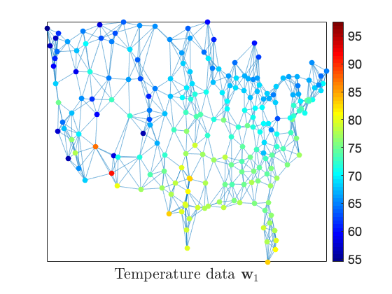
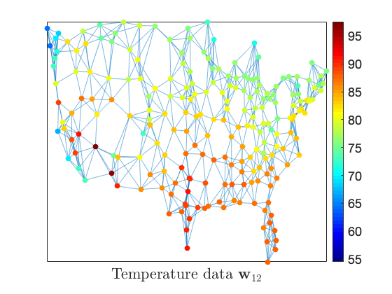
Figure 6: Presented on the left and right sides are the temperature data ${\bf w}_{1}$ and ${\bf w}_{12}$, where ${\bf w}_{i}$, $1\leq i\leq 24$, are the hourly temperature of 218 locations in the United States on August 1st, 2010.

In the section, we consider denoising the hourly temperature dataset collected at $218$ locations in the United States on August 1st, 2010, measured in Fahrenheit [5, 52]. The above real-world dataset is of size $218\times 24$, and it can be modelled as a time-varying signal ${\bf w}(i),1\leq i\leq 24$, on the product graph ${\mathcal{C}}\times{\mathcal{W}}$, where ${\mathcal{C}}:={\mathcal{C}}(24,\{1\})$ is the circulant graph with 24 vertices and generator $\{1\}$, and ${\mathcal{W}}$ is the undirected graph with $218$ locations as vertices and edges constructed by the 5 nearest neighboring algorithm, see Figure 6 for two snapshots of the dataset. Unlike in the simulation in the last subsection, the above time-varying signal ${\bf w}(t_{i}),1\leq i\leq 24$, is not necessarily to be governed by a different equation of the form (5.3).

Given noisy temperature data

$$\widetilde{\bf w}_{i}={\bf w}_{i}+{\boldsymbol{\eta}}_{i},\ i=1,\ldots,24,$$

we propose the following denoising approach,

$$\widehat{\bf W}:={\rm arg}\min_{\bf Z}\|{\bf Z}-{\widetilde{\bf W}}\|_{2}^{2}+\tilde{\alpha}{\bf Z}^{T}({\bf I}\otimes{\bf L}^{\rm sym}_{\mathcal{W}}){\bf Z}+\tilde{\beta}{\bf Z}^{T}({\bf L}_{\mathcal{C}}^{\rm sym}\otimes{\bf I}){\bf Z},$$ (5.13)

where $\widetilde{\bf W}$ is the vectorization of the noisy temperature data $\widetilde{\bf w}_{1},\ldots,\widetilde{\bf w}_{24}$ with noises ${\boldsymbol{\eta}}_{i},1\leq i\leq 24$ in (5.3) having their components randomly selected in $[-\eta,\eta]$ in a uniform distribution, ${\bf L}^{\rm sym}_{\mathcal{W}}$ and ${\bf L}_{\mathcal{C}}^{\rm sym}$ are normalized Laplacian matrices on the graph ${\mathcal{W}}$ and ${\mathcal{C}}$ respectively, and $\tilde{\alpha},\tilde{\beta}\geq 0$ are penalty constants in the vertex and temporal domains to be appropriately selected.

Set $\tilde{\bf S}_{1}={\bf I}\otimes{\bf L}^{\rm sym}_{\mathcal{W}}$, $\tilde{\bf S}_{2}={\bf L}_{\mathcal{C}}^{\rm sym}\otimes{\bf I}$ and ${\bf F}_{\tilde{\alpha},\tilde{\beta}}={\bf I}+\tilde{\alpha}\tilde{\bf S}_{1}+\tilde{\beta}\tilde{\bf S}_{2},\ \tilde{\alpha},\tilde{\beta}\geq 0$. One may verify that the explicit solution of the minimization problem (5.13) is given by $\widehat{\bf W}=({\bf F}_{\tilde{\alpha},\tilde{\beta}})^{-1}{\widetilde{\bf W}}$, and the proposed approach to denoise the temperature dataset becomes an inverse filtering procedure (3.1) with ${\bf H}$ and ${\bf b}$ replaced by ${\bf F}_{\tilde{\alpha},\tilde{\beta}}$ and $\widetilde{\bf W}$ respectively. In absence of notation, we still denote the IOPA algorithm (4.7) with $L=1$, the ICPA algorithm (4.16) with $K=1$ and the gradient descent method (3.13) with initial zero to implement the inverse filter procedure $\widetilde{\bf W}\longmapsto{\bf F}_{\tilde{\alpha},\tilde{\beta}}^{-1}\widetilde{\bf W}$ by IOPA1$(\tilde{\alpha},\tilde{\beta})$, ICPA1$(\tilde{\alpha},\tilde{\beta})$ and GD0$(\tilde{\alpha},\tilde{\beta})$ respectively.

In our simulations, we take

$$\tilde{\alpha}=\frac{\mathbb{E}\|{\bf Z}-{\widetilde{\bf W}}\|_{2}^{2}}{\mathbb{E}\big{(}{\widetilde{\bf W}^{T}}\tilde{\bf S}_{1}{\widetilde{\bf W}})}=\frac{1744\eta^{2}}{{\bf W}^{T}\tilde{\bf S}_{1}{\bf W}+1744\eta^{2}}$$

and

$$\tilde{\beta}=\frac{\mathbb{E}\|{\bf Z}-{\widetilde{\bf W}}\|_{2}^{2}}{\mathbb{E}(\widetilde{\bf W}^{T}\tilde{\bf S}_{2}\widetilde{\bf W})}=\frac{1744\eta^{2}}{{\bf W}^{T}\tilde{\bf S}_{2}{\bf W}+1744\eta^{2}}$$

to balance three terms in the regularization approach (5.13). Presented in Table 3 are the average over 1000 trials of the input signal-to-noise ratio ${\rm ISNR}$ and the output signal-to-noise ratio

$${\rm SNR}(m)=-20\log_{10}\frac{\|\widehat{\bf W}^{(m)}-{\bf W}\|_{2}}{\|{\bf W}\|_{2}},\ m\geq 1,\vspace{-0.6em}$$

which are used to measure the denoising performance of the IOPA1$(\tilde{\alpha},\tilde{\beta})$, ICPA1$(\tilde{\alpha},\tilde{\beta})$ and GD0$(\tilde{\alpha},\tilde{\beta})$ at the $m$th iteration, where $\widehat{\bf W}^{(\infty)}:=\widehat{\bf W}$ and $\widehat{\bf W}^{(m)},m\geq 1$, are outputs of the IOPA1$(\tilde{\alpha},\tilde{\beta})$ algorithm, or the ICPA1$(\tilde{\alpha},\tilde{\beta})$, or the GD0$(\tilde{\alpha},\tilde{\beta})$ at $m$-th iteration. From Table 3, we see that the Tikhonov regularization on the temporal-vertex domain has better performance on denoising the hourly temperature dataset than the Tikhonov regularization only either on the vertex domain (i.e. $\tilde{\beta}=0$) or on the temporal domain (i.e. $\tilde{\alpha}=0$) do. Also we observe that the temporal correlation has larger influence than the vertex correlation for small noise corruption $\eta\leq 10$, while the influence of the vertex correlation is more significant than the temporal correlation for the moderate and larger noise corruption.

Table 3: The average over 1000 trials of the signal-to-noise ratio ${\rm SNR}(m),m=1,2,4,6,\infty$ denoise the US hourly temperature dataset collected at $218$ locations on August 1st, 2010, where $\eta=35,20,10$.

m	1	2	4	6	$\infty$
$\eta$=35, ISNR= 11.5496
IOPA1($\tilde{\alpha}$, 0)	14.8906	16.2623	16.2499	16.2497	16.2497
IOPA1(0, $\tilde{\beta}$)	13.3792	15.7143	15.6925	15.6911	15.6911
IOPA1($\tilde{\alpha}$, $\tilde{\beta}$)	11.2985	18.1294	19.0536	19.0491	19.0487
ICPA1($\tilde{\alpha}$, 0)	14.2783	16.3118	16.2509	16.2498	16.2497
ICPA1(0, $\tilde{\beta}$)	14.0451	15.7475	15.6925	15.6911	15.6911
ICPA1($\tilde{\alpha}$, $\tilde{\beta}$)	9.8634	16.9294	19.0281	19.0486	19.0487
GD0($\tilde{\alpha}$, 0)	7.2407	13.2001	16.1692	16.2523	16.2497
GD0(0, $\tilde{\beta}$)	5.7453	10.8805	15.3374	15.7069	15.6911
GD0($\tilde{\alpha}$, $\tilde{\beta}$)	3.9579	7.8606	14.4865	17.9663	19.0487
$\eta$=20, ISNR= 16.4086
IOPA1($\tilde{\alpha}$, 0)	18.3271	20.2473	20.2470	20.2470	20.2470
IOPA1(0, $\tilde{\beta}$)	15.4936	20.4129	20.5195	20.5183	20.5183
IOPA1($\tilde{\alpha}$, $\tilde{\beta}$)	12.3927	21.0773	22.8075	22.8097	22.8095
ICPA1($\tilde{\alpha}$, 0)	17.5792	20.2654	20.2474	20.2470	20.2470
ICPA1(0, $\tilde{\beta}$)	16.73029	20.5223	20.5196	20.5183	20.5183
ICPA1($\tilde{\alpha}$, $\tilde{\beta}$)	10.7460	19.4217	22.7759	22.8092	22.8095
GD0($\tilde{\alpha}$, 0)	8.4637	15.7834	20.1310	20.2470	20.2470
GD0(0, $\tilde{\beta}$)	5.9817	11.7217	19.1824	20.4607	20.5183
GD0($\tilde{\alpha}$, $\tilde{\beta}$)	4.2594	8.4753	16.1761	21.0514	22.8095
$\eta$=10, ISNR=22.4320
IOPA1($\tilde{\alpha}$, 0)	23.3572	24.5564	24.5565	24.5565	24.5565
IOPA1(0, $\tilde{\beta}$)	16.9511	25.9123	26.4291	26.4284	26.4284
IOPA1($\tilde{\alpha}$, $\tilde{\beta}$)	14.2863	24.9125	26.9961	26.9990	26.9990
ICPA1($\tilde{\alpha}$, 0)	22.5720	24.5572	24.5565	24.5565	24.5565
ICPA1(0, $\tilde{\beta}$)	18.6319	26.2493	26.4294	26.4285	26.4284
ICPA1($\tilde{\alpha}$, $\tilde{\beta}$)	12.7428	23.3488	26.9816	26.9989	26.9990
GD0($\tilde{\alpha}$, 0)	11.7089	21.2276	24.5387	24.5566	24.5565
GD0(0, $\tilde{\beta}$)	6.2342	12.3916	22.7545	26.1414	26.4284
GD0($\tilde{\alpha}$, $\tilde{\beta}$)	4.9806	9.9239	19.2003	25.2121	26.9990

6 Conclusions and further works

Polynomial graph filters of multiple shifts are preferable for denoising and extracting features along different dimensions/directions for multidimensional graph signals, such as video or time-varying signals. A necessary condition is derived in this paper for a graph filter to be a polynomial of multiple shifts and the necessary condition is shown to be sufficient if the elements in the joint spectrum of multiple shifts are distinct. The design methodology of polynomial filters of multiple graph shifts and their inverses with specific features and physical interpretation for engineering applications will be discussed in our future works.

Some Tikhonov regularization approaches on the temporal-vertex domain to denoise a time-varying signal can be reformulated as an inverse filtering procedure for a polynomial graph filter of two shifts which represent the features on the temporal and vertex domain respectively. Two exponentially convergent iterative algorithms are introduced for the inverse filtering procedure of a polynomial graph filter, and each iteration of the proposed algorithms can be implemented in a distributed network, where each vertex is equipped with systems for limited data storage, computation power and data exchanging facility to its adjacent vertices. The proposed iterative algorithms are demonstrated to implement the inverse filtering procedure effectively and to have satisfactory performance on denoising multidimensional graph signals.

Appendix Appendix A Commutative graph shifts

Graph shifts are building blocks of a polynomial filter and the concept of commutative graph shifts ${\mathbf{S}}_{1},\ldots,{\mathbf{S}}_{d}$ is similar to the one-order delay $z_{1}^{-1},\ldots,z_{d}^{-1}$ in classical multi-dimensional signal processing. In Appendices A.1 and A.2, we introduce two illustrative families of commutative graph shifts on circulant/Cayley graphs and product graphs respectively, see also Subsections 5.2 and 5.3 for commutative graph shifts with specific features. For commutative graph shifts ${\mathbf{S}}_{1},\ldots,{\mathbf{S}}_{d}$, we define their joint spectrum (A.5) in Appendix A.3, which is crucial for us to develop the IOPA and ICPA algorithms in Section 4.

Commutativity of multiple graph shifts are essential to design polynomial graph filters with certain spectral characteristic. If a graph filter ${\bf H}$ is a polynomial of commutative multiple graph shifts ${\bf S}_{1},...,{\bf S}_{d}$, then it commutes with ${\bf S}_{k},1\leq k\leq d$, i.e., commutators $[{\bf H},{\bf S}_{k}]:={\bf H}{\bf S}_{k}-{\bf S}_{k}{\bf H}$ between ${\bf H}$ and ${\bf S}_{k},1\leq k\leq d$ are always the zero matrix,

$$[{\bf H},{\bf S}_{k}]={\bf 0},\ 1\leq k\leq d.\vspace{-0.6em}$$ (A.1)

The above necessary condition for a graph filter ${\bf H}$ to be a polynomial of ${\bf S}_{1},...,{\bf S}_{d}$ is not sufficient in general. For instance, one may verify that any filter ${\bf H}$ satisfies (A.1) with $d=1$ and ${\bf S}_{1}={\bf I}$, while ${\bf H}$ is not necessarily a polynomial $h({\bf I})=h(1){\bf I}$ of the identity matrix ${\bf I}$. For $d=1$, it is shown in [36, Theorem 1] that any filter satisfying (A.1) is a polynomial filter if the graph shift has distinct eigenvalues. In Theorem A.3 of Appendix A.4, we show that the necessary condition (A.1) is also sufficient under the additional assumption that elements in the joint spectrum of multiple graph shifts ${\mathbf{S}}_{1},\ldots,{\mathbf{S}}_{d}$ are distinct.

Let ${\mathcal{A}}$ be a Banach algebra of graph filters with its norm denoted by $\|\cdot\|_{\mathcal{A}}$. Our representative examples are the algebra of graph filters with Frobenius norm $\|\cdot\|_{F}$, operator algebras ${\mathcal{B}}(\ell^{p}),1\leq p\leq\infty$, on the space $\ell^{p}$ of all $p$-summable graph signals, Gröchenig-Schur algebras, Wiener algebra, Beurling algebras, Jaffard algebras and Baskakov-Gohberg-Sjöstrand algebras, see [15, 25, 42, 43, 44] for historical remarks and various applications. Denote the set of polynomials of commutative graph shifts ${\bf S}_{1},...,{\bf S}_{d}$ by ${\mathcal{P}}:={\mathcal{P}}({\bf S}_{1},\ldots,{\bf S}_{d})$. Under the assumption that ${\mathbf{S}}_{k}\in{\mathcal{A}},1\leq k\leq d$, one may verify that all polynomials of ${\bf S}_{1},...,{\bf S}_{d}$ reside in the Banach algebra ${\mathcal{A}}$ too, i.e., ${\mathcal{P}}\subset{\mathcal{A}}$. For any filter ${\mathbf{H}}\in{\mathcal{A}}$, define its distance to the polynomial set ${\mathcal{P}}$ of graph shifts ${\bf S}_{1},...,{\bf S}_{d}$ by

$${\rm dist}({\bf H},{\mathcal{P}})=\inf_{{\bf P}\in{\mathcal{P}}}\|{\bf H}-{\bf P}\|_{\mathcal{A}}.$$ (A.2)

Under the assumption that the elements of joint spectrum of multiple graph shifts ${\mathbf{S}}_{1},\ldots,{\mathbf{S}}_{d}$ are distinct, we obtain from Theorem A.3 that ${\rm dist}({\bf H},{\mathcal{P}})=0$ for any filter ${\bf H}\in{\mathcal{A}}$ satisfying (A.1). In Theorem A.4 of Appendix A.5, we establish some quantitative estimates to the distance ${\rm dist}({\bf H},{\mathcal{P}}),{\mathbf{H}}\in{\mathcal{A}}$, in terms of norms of commutators $[{\bf H},{\bf S}_{k}],1\leq k\leq d$, on an unweighted and undirected finite graph.

A.1 Commutative graph shifts on circulant graphs and Cayley graphs

Let ${\mathcal{C}}(N,Q)=(V_{N},E_{N}(Q))$ be the circulant graph of order $N$ generated by $Q=\{q_{1},\ldots,q_{M}\}$, where $1\leq q_{1}<\ldots<q_{M}<N/2$, see (5.1) and Figure 2. Observe that

$$E_{N}(Q)=\cup_{1\leq k\leq d}\big{\{}(i,i\pm q_{k}\ {\rm mod}\ N),i\in V_{N}\big{\}}.$$

Then the circulant graph ${\mathcal{C}}(N,Q)$ can be decomposed into a family of circulant graphs ${\mathcal{C}}(N,Q_{k})$ generated by $Q_{k}=\{q_{k}\},1\leq k\leq d$, and the symmetric normalized Laplacian matrix ${\bf L}_{{\mathcal{C}}(N,Q)}^{\rm sym}$ on ${\mathcal{C}}(N,Q)$ is the average of symmetric normalized Laplacian matrices ${\bf L}_{{\mathcal{C}}(N,Q_{k})}^{\rm sym}$ on ${\mathcal{C}}(N,Q_{k}),1\leq k\leq d$, i.e.,

$${\bf L}_{{\mathcal{C}}(N,Q)}^{\rm sym}=\frac{1}{d}\sum_{k=1}^{d}{\bf L}_{{\mathcal{C}}(N,Q_{k})}^{\rm sym},\vspace{-.4em}$$

where $Q_{k}=\{q_{k}\},1\leq k\leq d$. In the following proposition, we establish the commutativity of ${\bf L}_{{\mathcal{C}}(N,Q_{k})}^{\rm sym},1\leq k\leq d$.

Proposition A.1.

The symmetric normalized Laplacian matrices ${\bf L}_{{\mathcal{C}}(N,Q_{k})}^{\rm sym}$ of the circulant graphs ${\mathcal{C}}(N,Q_{k}),1\leq k\leq d$, are commutative graph shifts on the circulant graph ${\mathcal{C}}(N,Q)$.

Proof.

Clearly ${\bf L}_{{\mathcal{C}}(N,Q_{k})}^{\rm sym},1\leq k\leq d$, are graph shifts on the circulant graph ${\mathcal{C}}(N,Q)$. Define

$${\bf B}=(b({i-j\ {\rm mod}\ N}))_{1\leq i,j\leq N},$$

where $b(0)=\cdots=b({N-2})=0$ and $b({N-1})=1$. Then one may verify that

$${\bf L}_{{\mathcal{C}}(N,Q_{k})}^{\rm sym}={\bf I}-\frac{1}{2}({\bf B}^{q_{k}}+{\bf B}^{-q_{k}})=-\frac{1}{2}{\bf B}^{-q_{k}}({\bf B}^{q_{k}}-{\bf I})^{2},\vspace{-.4em}$$

where $1\leq k\leq d$. Therefore for $1\leq k,k^{\prime}\leq d$,

$${\bf L}_{{\mathcal{C}}(N,Q_{k^{\prime}})}^{\rm sym}{\bf L}_{{\mathcal{C}}(N,Q_{k})}^{\rm sym}=\frac{1}{4}{\bf B}^{-q_{k}-q_{k^{\prime}}}({\bf B}^{q_{k}}-{\bf I})^{2}({\bf B}^{q_{k^{\prime}}}-{\bf I})^{2}={\bf L}_{{\mathcal{C}}(N,Q_{k})}^{\rm sym}{\bf L}_{{\mathcal{C}}(N,Q_{k^{\prime}})}^{\rm sym}.$$

This completes the proof. ∎

Following the proof of Proposition A.1, we have that the adjacent matrices $2({\bf I}-{\bf L}_{{\mathcal{C}}(N,Q_{k})}^{\rm sym})={\bf B}^{q_{k}}+{\bf B}^{-q_{k}}$ of the circulant graphs ${\mathcal{C}}(N,Q_{k}),1\leq k\leq d$, (and their linear combinations) are commutative graph shifts on the circulant graph ${\mathcal{C}}(N,Q)$.

Connected circulant graphs are regular undirected Cayley graphs of finite cyclic groups. In general, for an Abelian group $G$ generated by a finite set $S$ of non-identity elements and a color assignment $c_{s}$ to each element $s\in S$, the Cayley graph ${\mathcal{G}}$ is defined to have elements in the group $G$ as its vertices and directed edges of color $c_{s}$ between vertices $g$ to $gs$ in $G$. For the case that the generator $S$ is symmetric (i.e., $S^{-1}=S$) and the same color is assigned for any element in the generator $S$ and its inverse (i.e., $c_{s}=c_{s^{-1}},s\in S$), one may verify that the Cayley graph ${\mathcal{G}}$ is a regular undirected graph, it can be decomposed into a family of regular subgraphs ${\mathcal{G}}_{s},s\in S_{1}$ with the same colored edges,

$${\mathcal{G}}=\cup_{s\in S_{1}}{\mathcal{G}}_{s},$$

and the adjacent matrix of the Cayley graph is the summation of the adjacent matrices associated with the regular subgraphs ${\mathcal{G}}_{s},s\in S_{1}$, where the subset $S_{1}\subset S$ is chosen so that different colors are assigned for distinct elements in $S_{1}$ and all colors $c_{s},s\in S$ are represented in $S_{1}$. Furthermore, similar to the commutativity for symmetric normalized Laplacian matrices in Proposition A.1, we can show that the adjacent matrices, Laplacian matrices, symmetric normalized Laplacian matrices associated with the regular subgraphs ${\mathcal{G}}_{s},s\in S_{1}$, are commutative graph shifts of the Cayley graph ${\mathcal{G}}$.

A.2 Commutative graph shifts on Cartesian product graphs

Let ${\mathcal{G}}_{1}=(V_{1},E_{1})$ and ${\mathcal{G}}_{2}=(V_{2},E_{2})$ be two finite graphs with adjacency matrices ${\bf A}_{1}$ and ${\bf A}_{2}$. Their Cartesian product graph ${\mathcal{G}}_{1}\times{\mathcal{G}}_{2}$ has vertex set $V_{1}\times V_{2}$ and adjacency matrix given by ${\bf A}={\bf A}_{1}\otimes{\bf I}_{\#V_{2}}+{\bf I}_{\#V_{1}}\otimes{\bf A}_{2}$ [14, 28]. Shown in Figure 7 is an illustrative example of product graphs and the time-varying graph signal ${\bf X}$ can be considered as a signal on the Cartesian product graph ${\mathcal{T}}\times{\mathcal{G}}$, see Subsection 5.2.

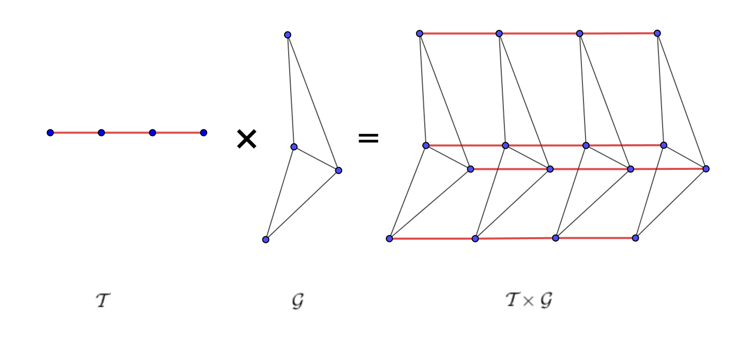
Figure 7: Cartesian product ${\mathcal{T}}\times{\mathcal{G}}$ of a line graph $\mathcal{T}$ and an undirected graph $\mathcal{G}$.

Denote symmetric normalized Laplacian matrices and orders of the graph ${\mathcal{G}}_{i},i=1,2$ by ${\bf L}_{i}^{\rm sym}$ and $N_{i}$ respectively. By the mixed-product property

$$({\bf A}\otimes{\bf B})({\bf C}\otimes{\bf D})=({\bf AC})\otimes({\bf BD})\vspace{-.4em}$$ (A.3)

for Kronecker product of matrices ${\bf A},{\bf B},{\bf C},{\bf D}$ of appropriate sizes [27], one may verify that ${\bf L}_{1}^{\rm sym}\otimes{\bf I}_{N_{2}}$ and ${\bf I}_{N_{1}}\otimes{\bf L}_{2}^{\rm sym}$ are graph filters of the Cartesian product graph ${\mathcal{G}}_{1}\times{\mathcal{G}}_{2}$. In the following proposition, we show that they are commutative.

Proposition A.2.

Let ${\mathcal{G}}_{1}=(V_{1},E_{1})$ and ${\mathcal{G}}_{2}=(V_{2},E_{2})$ be two finite graphs with normalized Laplacian matrices ${\bf L}_{1}^{\rm sym}$ and ${\bf L}_{2}^{\rm sym}$ respectively. Then ${\bf L}_{1}^{\rm sym}\otimes{\bf I}_{\#V_{2}}$ and ${\bf I}_{\#V_{1}}\otimes{\bf L}_{2}^{\rm sym}$ are commutative graph shifts of the Cartesian product graph ${\mathcal{G}}_{1}\times{\mathcal{G}}_{2}$.

Proof.

Let $N_{i}=\#V_{i},i=1,2$ and set ${\bf C}_{1}={\bf L}_{1}^{\rm sym}\otimes{\bf I}_{N_{2}}$ and ${\bf C}_{2}={\bf I}_{N_{1}}\otimes{\bf L}_{2}^{\rm sym}$. By the mixed-product property (A.3) of Kronecker product, Then

$${\bf C_{1}}{\bf C}_{2}={\bf L}_{1}^{\rm sym}\otimes{\bf L}_{2}^{\rm sym}={\bf C}_{2}{\bf C}_{1}.$$

∎

A.3 Joint spectrum of commutative shifts

Let ${\bf S}_{1},...,{\bf S}_{d}$ be commutative graph shifts. An important property in [18, Theorem 2.3.3] is that they can be upper-triangularized simultaneously over ${\mathbb{C}}$, i.e.,

$$\widehat{\bf S}_{k}={\bf U}{\bf S}_{k}{\bf U}^{\rm H},\ 1\leq k\leq d,$$ (A.4)

are upper triangular matrices for some unitary matrix ${\bf U}$. Write $\widehat{\bf S}_{k}=(\widehat{S}_{k}(i,j))_{1\leq i,j\leq N},1\leq k\leq d$, and set

$$\Lambda=\big{\{}\boldsymbol{\lambda}_{i}=\big{(}\widehat{S}_{1}(i,i),...,\widehat{S}_{d}(i,i)\big{)},1\leq i\leq N\big{\}}\subset{\mathbb{C}}^{d}.\vspace{-.2em}$$ (A.5)

As $\widehat{S}_{k}(i,i),1\leq i\leq N$, are complex eigenvalues of ${\bf S}_{k},\ 1\leq k\leq d$, we call $\Lambda$ as the joint spectrum of ${\bf S}_{1},\ldots,{\bf S}_{d}$. The joint spectrum $\Lambda$ of commutative shifts ${\bf S}_{1},\ldots,{\bf S}_{d}$ plays an essential role in Section 4 in the construction of optimal polynomial approximation filters and Chebyshev polynomial approximation filters to the inverse filter of a polynomial filter of ${\bf S}_{1},...,{\bf S}_{d}$.

We remark that a sufficient condition for the graph shifts ${\bf S}_{1},\ldots,{\bf S}_{d}$ to be commutative is that they can be diagonalized simultaneously, i.e., there exists a nonsingular matrix ${\bf P}$ such that ${\bf P}^{-1}{\bf S}_{k}{\bf P},1\leq k\leq d$, are diagonal matrices, which a necessary condition is that they can be upper-triangularized simultaneously, see (A.4).

A.4 Polynomial graph filters of commutative filters

Let ${\bf S}_{1},...,{\bf S}_{d}$ be commutative graph shifts. In the following theorem, we show that the necessary condition (A.1) for a filter to be a polynomial of multiple graph shifts is also sufficient under the additional assumption that the joint eigenvalues $\boldsymbol{\lambda}_{i},1\leq i\leq N$, in the joint spectrum $\Lambda$ in (A.5) are distinct.

Theorem A.3.

Let ${\bf S}_{1},\ldots,{\bf S}_{d}$ be commutative graph filters, and the joint spectrum ${\Lambda}$ be as in (A.5). If all elements ${\boldsymbol{\lambda}}_{i},1\leq i\leq N$, in the set ${\Lambda}$ are distinct, then any graph filter ${\bf H}$ satisfying (A.1) is a polynomial of ${\bf S}_{1},...,{\bf S}_{d}$, i.e., ${\bf H}=h({\bf S}_{1},...,{\bf S}_{d})$ for some polynomial $h$.

Proof.

Let ${\bf U}$ be the unitary matrix in (A.4), $\widehat{\bf S}_{1},\ldots,\widehat{\bf S}_{d}$ be upper triangular matrices in (A.4), and $\widehat{\bf H}={\bf U}{\bf H}{\bf U}^{\rm H}=(\widehat{H}(i,j))_{1\leq i,j\leq N}$. By the assumption on the set $\Lambda$, there exist an interpolating polynomial $h$ such that

$$h(\widehat{S}_{1}(i,i),...,\widehat{S}_{d}(i,i))=\widehat{H}(i,i),\ 1\leq i\leq N,\vspace{-0.6em}$$ (A.6)

see [4, Theorem 1 on p. 58]. Set

$${\bf F}={\bf U}\big{(}{\bf H}-h({\bf S}_{1},...,{\bf S}_{d})\big{)}{\bf U}^{\rm H}=\widehat{\bf H}-h(\widehat{\bf S}_{1},\ldots,\widehat{\bf S}_{d}).\vspace{-0.6em}$$ (A.7)

Then it suffices to prove that ${\bf F}$ is the zero matrix.

Write ${\bf F}=(F(i,j))_{1\leq i,j\leq N}$. By (A.1), we have that ${\bf F}\widehat{\bf S}_{k}=\widehat{\bf S}_{k}{\bf F}$ for all $1\leq k\leq d$. This together with the upper triangular property for $\widehat{\bf S}_{k},1\leq k\leq d$, implies that

$$\sum_{l=1}^{j}F(i,l)\widehat{S}_{k}(l,j)=\sum_{l=i}^{N}\widehat{S}_{k}(i,l)F(l,j),\ 1\leq i,j\leq N.\vspace{-0.5em}$$ (A.8)

By the assumption on $\Lambda$, we can find $1\leq k(i,j)\leq d$ for any $1\leq i\neq j\leq N$ such that

$$\widehat{S}_{k(i,j)}(i,i)\neq\widehat{S}_{k(i,j)}(j,j).\vspace{-0.6em}$$ (A.9)

Now we apply (A.8) and (A.9) to prove

$${F}(i,j)=0\vspace{-0.6em}$$ (A.10)

by induction on $j=1,\ldots,N$ and $i=N,\ldots,1$.

For $i=N$ and $j=1$, applying (A.8) with $k$ replaced by $k(N,1)$, we obtain

$$F(N,1)\widehat{S}_{k(N,1)}(1,1)=\widehat{S}_{k(N,1)}(N,N)F(N,1),\vspace{-0.4em}$$

which together with (A.9) proves (A.10) for $(i,j)=(N,1)$. Inductively we assume that the conclusion (A.10) for all pairs $(i,j)$ satisfying either $1\leq j\leq j_{0}$ and $i=i_{0}$, or $1\leq j\leq N$ and $i_{0}<i\leq N$.

For the case that $j_{0}<i_{0}-1$, we have

$$F(i_{0},j_{0}+1)\widehat{S}_{k(i_{0},j_{0}+1)}(j_{0}+1,j_{0}+1)=\sum_{l=1}^{j_{0}+1}F(i_{0},l)\hat{S}_{k(i_{0},j_{0}+1)}(l,j_{0}+1)$$

$$= \sum_{l=i_{0}}^{N}\widehat{S}_{k(i_{0},j_{0}+1)}(i_{0},l)F(l,j_{0}+1)=\widehat{S}_{k(i_{0},j_{0}+1)}(i_{0},i_{0})F(i_{0},j_{0}+1),$$

where the first and third equalities hold by the inductive hypothesis and the second equality is obtained from (A.8) with $k$ replaced by $k(i_{0},j_{0}+1)$. This together with (A.9) proves the conclusion (A.10) for $i=i_{0}$ and $j=j_{0}+1\leq i_{0}-1$, and hence the inductive proof can proceed for the case that $j_{0}<i_{0}-1$.

For the case that $j_{0}=i_{0}-1$, it follows from the construction of the polynomial $h$ and the upper triangular property for $\widehat{\bf S}_{k},1\leq k\leq d$, that the diagonal entries of ${\bf F}$ are

$$\widehat{H}(i,i)-h(\widehat{S}_{1}(i,i),...,\widehat{S}_{d}(i,i))=0,\ 1\leq i\leq N\vspace{-0.4em}$$

by (A.6). Hence the conclusion (A.10) holds for $i=i_{0}$ and $j=j_{0}+1$, and hence the inductive proof can proceed for the case that $j_{0}=i_{0}-1$.

For the case that $i_{0}\leq j_{0}\leq N-1$, we can follow the argument used in the proof for the case that $j_{0}<i_{0}-1$ to establish the conclusion (A.10) for $i=i_{0}$ and $j=j_{0}+1\leq N$, and hence the inductive proof can proceed for the case that $i_{0}\leq j_{0}\leq N-1$.

For the case that $j_{0}=N$ and $i_{0}\geq 2$, we obtain

$$F(i_{0}-1,1)\widehat{S}_{k(i_{0}-1,1)}(1,1)=\sum_{l=i_{0}-1}^{N}\widehat{S}_{k(i_{0}-1,l)}(i_{0}-1,l)F(l,1)=\widehat{S}_{k(i_{0}-1,1)}(i_{0}-1,i_{0}-1)F(i_{0}-1,1),$$

where the first equality follows from (A.8) with $k$ replaced by $k(i_{0}-1,1)$ and the second equality holds by the inductive hypothesis. This together with (A.9) proves the conclusion (A.10) for $i=i_{0}-1$ and $j=1$, and hence the inductive proof can proceed for the case that $j_{0}=N$ and $i_{0}\geq 2$.

For the case that $j_{0}=N$ and $i_{0}=1$, the inductive proof of the zero matrix property for the matrix ${\bf F}$ is complete. This completes the inductive proof. ∎

A.5 Distance between a graph filter and the set of polynomial of commutative graph shifts

Let ${\mathcal{G}}=(V,E)$ be a connected, unweighted and undirected finite graph, ${\mathcal{A}}$ be a Banach algebra of graph filters on the graph ${\mathcal{G}}$ with norm denoted by $\|\cdot\|_{\mathcal{A}}$, ${\bf S}_{1},\ldots,{\bf S}_{d}$ be nonzero commutative graph shifts in ${\mathcal{A}}$, and ${\mathcal{P}}$ be the set of all polynomial filters of graph shifts In this Appendix, we consider estimating the distance ${\rm dist}({\bf H},{\mathcal{P}})$ in (A.2) between a graph filter ${\bf H}$ and the set ${\mathcal{P}}$ of polynomial filters.

Theorem A.4.

If the commutative graph shifts ${\mathbf{S}}_{1},\ldots,{\bf S}_{d}$ can be diagonalized simultaneously by a unitary matrix and elements in their joint spectrum $\Lambda$ are distinct, then there exist positive constants $C_{0}$ and $C_{1}$ such that

$$C_{0}\Big{(}\sum_{k=1}^{d}\|[{\bf H},{\bf S}_{k}]\|_{\mathcal{A}}^{2}\Big{)}^{1/2}\leq{\rm dist}({\bf H},{\mathcal{P}})\leq C_{1}\Big{(}\sum_{k=1}^{d}\|[{\bf H},{\bf S}_{k}]\|_{\mathcal{A}}^{2}\Big{)}^{1/2},\ {\bf H}\in{\mathcal{A}},$$ (A.11)

where $[{\bf H},{\bf S}_{k}]={\bf H}{\bf S}_{k}-{\bf S}_{k}{\bf H},1\leq k\leq d$.

Proof.

Take ${\bf H}\in{\mathcal{A}}$. For any ${\bf P}\in{\mathcal{P}}$, we have

$$\|[{\bf H},{\bf S}_{k}]\|_{\mathcal{A}}\leq\|({\bf H}-{\mathbf{P}}){\bf S}_{k}\|_{\mathcal{A}}+\|{\bf S}_{k}({\bf H}-{\mathbf{P}})\|_{\mathcal{A}}\leq 2\|{\bf S}_{k}\|_{\mathcal{A}}\|{\bf H}-{\bf P}\|_{\mathcal{A}},\ 1\leq k\leq d.$$

Therefore

$${\rm dist}({\bf H},{\mathcal{P}})\geq\max_{1\leq k\leq d}\frac{\|[{\bf H},{\bf S}_{k}]\|_{\mathcal{A}}}{2\|{\bf S}_{k}\|_{\mathcal{A}}},$$

and the first inequality in (A.11) follows.

Now we prove the second inequality in (A.11). Let ${\bf U}$ be the unitary matrix to diagonalize ${\mathbf{S}}_{1},\ldots,{\bf S}_{d}$ simultaneously, i.e., (A.4) holds for some diagonal matrices $\widehat{\bf S}_{k}={\rm diag}(\widehat{S}(i,i))_{i\in V},1\leq k\leq d$. Then one may verify that polynomial filters of graph shifts ${\mathbf{S}}_{1},\ldots,{\bf S}_{d}$ can also be diagonalized by the unitary matrix ${\bf U}$. Moreover by the distinct assumption on elements in the joint spectrum $\Lambda$ of the graph shifts, we have

$${\mathcal{P}}=\{{\bf U}^{\rm H}{\bf D}{\bf U},\ {\bf D}\ {\rm are\ diagonal\ matrices}\}.$$ (A.12)

Set ${\bf U}{\bf H}{\bf U}^{\rm H}=(\widehat{H}(i,j))_{i,j\in V}$. and denote the Frobenius norm of a matrix ${\bf A}$ by $\|{\bf A}\|_{F}$. Therefore it follows from (A.12) that

$$\inf_{{\bf P}\in{\mathcal{P}}}\|{\bf H}-{\bf P}\|_{F}=\inf_{{\bf D}\ {\rm are\ diagonal\ matrices}}\|{\bf U}^{\rm H}{\bf H}{\bf U}-{\bf D}\|_{F}=\Big{(}\sum_{i,j\in V,j\neq i}|\widehat{H}(i,j)|^{2}\Big{)}^{1/2}.$$ (A.13)

On the other hand, we have

$${\bf U}[{\bf H},{\bf S}_{k}]{\bf U}^{\rm H}=\Big{(}\widehat{H}(i,j)(\widehat{S}_{k}(j,j)-\widehat{S}_{k}(i,i))\Big{)}_{i,j\in V},\ 1\leq k\leq d.$$

This implies that

$$\sum_{k=1}^{d}\|[{\bf H},{\bf S}_{k}]\|_{F}^{2} \hskip-5.78172pt= \hskip-5.78172pt\sum_{k=1}^{d}\|{\bf U}^{\rm H}|[{\bf H},{\bf S}_{k}]{\bf U}\|_{F}^{2}=\sum_{i,j\in V,j\neq i}|\widehat{H}(i,j)|^{2}\Big{(}\sum_{k=1}^{d}\big{|}\widehat{S}_{k}(j,j)-\widehat{S}_{k}(i,i)\big{|}^{2}\Big{)}$$ (A.14)

$$\hskip-5.78172pt\geq \hskip-5.78172pt\inf_{i,j\in V,j\neq i}\Big{(}\sum_{k=1}^{d}\big{|}\widehat{S}_{k}(j,j)-\widehat{S}_{k}(i,i)\big{|}^{2}\Big{)}\times\inf_{{\bf P}\in{\mathcal{P}}}\|{\bf H}-{\bf P}\|_{F}^{2},$$

where the last inequality follows from (A.13). Then the second inequality in (A.11) follows from (A.14), the equivalence of norms on a finite-dimensional linear space and the distinct assumption on the joint spectrum $\Lambda$. ∎

We believe that the estimate (A.11) should hold without the simultaneous diagonalization assumption on commutative graph shifts ${\bf S}_{1},\ldots,{\bf S}_{d}$.

Acknowledgement:  This work is partially supported by the National Natural Science Foundation of China (61761011, 62171146, 12171490) and the National Science Foundation (DMS-1816313). The authors would like to thank anonymous reviewers to provide many constructive comments for the improvement of the paper. On behalf of all authors, the corresponding author states that there is no conflict of interest.

References

- [1] A. W. Bohannon, B. M. Sadler, and R. V. Balan, “A filtering framework for time-varying graph signals,” in Vertex-Frequency Analysis of Graph Signals, Springer, pp. 341-376, 2019.
- [2] S. Chen, A. Sandryhaila, and J. Kovačević, “Distributed algorithm for graph signal inpainting,” 2015 IEEE International Conference on Acoustics, Speech and Signal Processing (ICASSP), Brisbane, QLD, 2015, pp. 3731-3735.
- [3] S. Chen, A. Sandryhaila, J. M. F. Moura, and J. Kovačević, “Signal recovery on graphs: variation minimization,” IEEE Trans. Signal Process., vol. 63, no. 17, pp. 4609-4624, Sept. 2015.
- [4] W. Cheney and W. Light. A Course in Approximation Theory, Brook/Cole Publishing Company, 2000.
- [5] C. Cheng, N. Emirov, and Q. Sun, “Preconditioned gradient descent algorithm for inverse filtering on spatially distributed networks”, IEEE Signal Process. Lett., vol. 27, pp. 1834-1838, Oct. 2020.
- [6] C. Cheng, J. Jiang, N. Emirov, and Q. Sun, “Iterative Chebyshev polynomial algorithm for signal denoising on graphs,” in Proceeding 13th Int. Conf. on SampTA, Bordeaux, France, Jul. 2019, pp. 1-5.
- [7] C. Cheng, Y. Jiang, and Q. Sun, “Spatially distributed sampling and reconstruction,” Appl. Comput. Harmon. Anal., vol. 47, no. 1, pp. 109-148, Jul. 2019.
- [8] F. Chung, Spectral Graph Theory, CBMS Regional Conference Series in Mathematics, No. 92. Providence, RI, Amer. Math. Soc., 1997.
- [9] M. Coutino, E. Isufi, and G. Leus, “Advances in distributed graph filtering,” IEEE Trans. Signal Process., vol. 67, no. 9, pp. 2320-2333, May 2019.
- [10] V. N. Ekambaram, G. C. Fanti, B. Ayazifar, and K. Ramchandran, “Circulant structures and graph signal processing,” in Proc. IEEE Int. Conf. Image Process., 2013, pp. 834-838.
- [11] V. N. Ekambaram, G. C. Fanti, B. Ayazifar, and K. Ramchandran, “Multiresolution graph signal processing via circulant structures,” in Proc. IEEE Digital Signal Process. Signal Process. Educ. Meeting (DSP/SPE), 2013, pp. 112-117.
- [12] J. Fan, C. Tepedelenlioglu, and A. Spanias, “Graph filtering with multiple shift matrices,” in IEEE International Conference on Acoustics, Speech and Signal Processing (ICASSP ), pp. 3557-3561, May 2019.
- [13] A. Gavili and X. Zhang, “On the shift operator, graph frequency, and optimal filtering in graph signal processing,” IEEE Trans. Signal Process., vol. 65, no. 23, pp. 6303-6318, Dec. 2017.
- [14] F. Grassi, A. Loukas, N. Perraudin, and B. Ricaud, “A time-vertex signal processing framework: scalable processing and meaningful representations for time-series on graphs,” IEEE Trans. Signal Process., vol. 66, no. 3, pp. 817-829, Feb. 2018.
- [15] K. Gröchenig, Wiener’s lemma: theme and variations, an introduction to spectral invariance and its applications, In Four Short Courses on Harmonic Analysis: Wavelets, Frames, Time-Frequency Methods, and Applications to Signal and Image Analysis, edited by P. Massopust and B. Forster, Birkhauser, Boston 2010.
- [16] D. K. Hammod, P. Vandergheynst, and R. Gribonval, “Wavelets on graphs via spectral graph theory,” Appl. Comput. Harmon. Anal., vol. 30, no. 4, pp. 129-150, Mar. 2011.
- [17] R. Hebner, “The power grid in 2030,” IEEE Spectrum, vol. 54, no. 4, pp. 50-55, Apr. 2017.
- [18] R. A. Horn and C. R. Johnson. Matrix Analysis, Cambridge University Press, 2012.
- [19] E. Isufi, A. Loukas, A. Simonetto, and G. Leus, “Autoregressive moving average graph filtering,” IEEE Trans. Signal Process., vol. 65, no. 2, pp. 274-288, Jan. 2017.
- [20] E. Isufi, A. Loukas, N. Perraudin, and G. Leus, “Forecasting time series with VARMA recursions on graphs,” IEEE Trans. Signal Process., vol. 67, no. 18, pp. 4870-4885, Sept. 2019.
- [21] J. Jiang, C. Cheng, and Q. Sun, “Nonsubsampled graph filter banks: Theory and distributed algorithms,” IEEE Trans. Signal Process., vol. 67, no. 15, pp. 3938-3953, Aug. 2019.
- [22] J. Jiang, D. B. Tay, Q. Sun, and S. Ouyang, “Design of nonsubsampled graph filter banks via lifting schemes,” IEEE Signal Process. Lett., vol. 27, pp. 441-445, Feb. 2020.
- [23] M. S. Kotzagiannidis and P. L. Dragotti, “Splines and wavelets on circulant graphs,” Appl. Comput. Harmon. Anal., vol. 47, no. 2, pp. 481-515, Sept. 2019.
- [24] M. S. Kotzagiannidis and P. L. Dragotti, “Sampling and reconstruction of sparse signals on circulant graphs – an introduction to graph-FRI,” Appl. Comput. Harmon. Anal., vol. 47, no. 3, pp. 539-565, Nov. 2019.
- [25] I. Krishtal, Wiener’s lemma: pictures at exhibition, Rev. Un. Mat. Argentina, 52(2011), 61–79.
- [26] T. Kurokawa, T. Oki, and H. Nagao, “Multi-dimensional graph Fourier transform,” arXiv: 1712.07811, Dec. 2017.
- [27] A. J. Laub, Matrix Analysis for Scientists and Engineers, PA, Philadelphia, SIAM, 2005.
- [28] A. Loukas and D. Foucard, “Frequency analysis of time-varying graph signals,” in IEEE Global Conf. Signal Inf. Process. (GlobalSIP), 2016, pp. 346-350.
- [29] K. Lu, A. Ortega, D. Mukherjee and Y. Chen, “Efficient rate-distortion approximation and transform type selection using Laplacian operators,” in 2018 Picture Coding Symposium (PCS), San Francisco, CA, 2018, pp. 76-80.
- [30] S. K. Narang and A. Ortega, “Perfect reconstruction two-channel wavelet filter banks for graph structured data,” IEEE Trans. Signal Process., vol. 60, no. 6, pp. 2786-2799, Jun. 2012.
- [31] P. Nathanael, J. Paratte, D. Shuman, L. Martin, V. Kalofolias, P. Vandergheynst, and D. K. Hammond, “GSPBOX: A toolbox for signal processing on graphs,” arXiv:1408.5781, Aug. 2014.
- [32] M. Onuki, S. Ono, M. Yamagishi, and Y. Tanaka, “Graph signal denoising via trilateral filter on graph spectral domain,” IEEE Trans. Signal Inf. Process. Netw., vol. 2, no. 2, pp. 137-148, Jun. 2016.
- [33] A. Ortega, P. Frossard, J. Kovačević, J. M. F. Moura, and P. Vandergheynst, “Graph signal processing: Overview, challenges, and applications,” Proc. IEEE, vol. 106, no. 5, pp. 808-828, May 2018.
- [34] G. M. Phillips, Interpolation and Approximation by Polynomials, CMS Books Math., Springer-Verlag, 2003.
- [35] K. Qiu, X. Mao, X. Shen, X. Wang, T. Li, and Y. Gu, “Time-varying graph signal reconstruction,” IEEE J. Sel. Topics Signal Process., vol. 11, no. 6, pp. 870-883, Sept. 2017.
- [36] A. Sandryhaila and J. M. F. Moura, “Discrete signal processing on graphs,” IEEE Trans. Signal Process., vol. 61, no. 7, pp. 1644-1656, Apr. 2013.
- [37] A. Sandryhaila and J. M. F. Moura, “Discrete signal processing on graphs: Frequency analysis,” IEEE Trans. Signal Process., vol. 62, no. 12, pp. 3042-3054, Jun. 2014.
- [38] A. Sandryhaila and J. M. F. Moura, “Big data analysis with signal processing on graphs: Representation and processing of massive data sets with irregular structure,” IEEE Signal Process. Mag., vol. 31, no. 5, pp. 80-90, Sept. 2014.
- [39] A. Sakiyama, K. Watanabe, Y. Tanaka, and A. Ortega, “Two-channel critically sampled graph filter banks with spectral domain sampling,” IEEE Trans. Signal Process., vol. 67, no. 6, pp. 1447-1460, Mar. 2019.
- [40] S. Segarra, A. G. Marques, and A. Ribeiro, “Optimal graph-filter design and applications to distributed linear network operators,” IEEE Trans. Signal Process., vol. 65, no. 15, pp. 4117-4131, Aug. 2017.
- [41] X. Shi, H. Feng, M. Zhai, T. Yang, and B. Hu, “Infinite impulse response graph filters in wireless sensor networks,” IEEE Signal Process. Lett., vol. 22, no. 8, pp. 1113-1117, Aug. 2015.
- [42] C. E. Shin and Q. Sun, Wiener’s lemma: localization and various approaches, Appl. Math. J. Chinese Univ., 28(2013), pp. 465–484.
- [43] C. E. Shin and Q. Sun, Polynomial control on stability, inversion and powers of matrices on simple graphs, J. Funct. Anal., 276(2019), pp. 148–182.
- [44] C. E. Shin and Q. Sun, Differential subalgebras and norm-controlled inversion, In Operator Theory, Operator Algebras and Their Interactions with Geometry and Topology, Birkhauser, 2020, pp. 467–485.
- [45] D. I. Shuman, S. K. Narang, P. Frossard, A. Ortega, and P. Vandergheynst, “The emerging field of signal processing on graphs: Extending high-dimensional data analysis to networks and other irregular domains,” IEEE Signal Process. Mag., vol. 30, no. 3, pp. 83-98, May 2013.
- [46] D. I. Shuman, P. Vandergheynst, D. Kressner, and P. Frossard, “Distributed signal processing via Chebyshev polynomial approximation,” IEEE Trans. Signal Inf. Process. Netw., vol. 4, no. 4, pp. 736-751, Dec. 2018.
- [47] O. Teke and P. P. Vaidyanathan, “Extending classical multirate signal processing theory to graphs Part II: M-channel filter banks,” IEEE Trans. Signal Process., vol. 65, no. 2, pp. 423-437, Jan. 2017.
- [48] D. Valsesia, G. Fracastoro, and E. Magli, “Deep graph-convolutional image denoising,” IEEE Trans. Image Process., vol. 29, pp. 8226-8237, Aug. 2020.
- [49] W. Waheed and D. B. H. Tay, “Graph polynomial filter for signal denoising,” IET Signal Process., vol. 12, no. 3, pp. 301-309, Apr. 2018.
- [50] J. Yi and L. Chai, “Graph filter design for multi-agent system consensus,” in IEEE 56th Annual Conference on Decision and Control (CDC), Melbourne, VIC, 2017, pp. 1082-1087.
- [51] J. Yick, B. Mukherjee, and D. Ghosal, “Wireless sensor network survey,” Comput. Netw., vol. 52, no. 12, pp. 2292-2330, Aug. 2008.
- [52] J. Zeng, G. Cheung, and A. Ortega, “Bipartite approximation for graph wavelet signal decomposition,” IEEE Trans. Signal Process., vol. 65, no. 20, pp. 5466-5480, Oct. 2017.