Fluctuation theorems for multiple co-evolving systems

Abstract

All previously derived thermodynamic fluctuation theorems (FTs) that concern multiple co-evolving systems have required that each system can only change its state during an associated pre-fixed, limited set of times. However, in many real-world cases the times when systems change their states are randomly determined, e.g., in almost all biological examples of co-evolving systems. Such randomness in the timing drastically modifies the thermodynamics. Here I derive FTs that apply whether or not the timing is random. These FTs provide new versions of the second law, and of all conventional thermodynamic uncertainty relations (TURs). These new results are often stronger than the conventional versions, which ignore how an overall system may decompose into a set of co-evolving systems. In addition, the new TURs often bound entropy production (EP) of the overall system even if none of the criteria for a conventional TUR (e.g., being a nonequilibrium steady state) hold for that overall system. In some cases the new FTs also provide a new type of speed limit theorem, and in some cases they also provide nontrivial upper bounds on expected EP of systems. I use a standard example of ligand detectors in a cell wall to illustrate these results.

I Introduction

Some of the most important results in stochastic thermodynamics are the fluctuation theorems (FTs) seifert2012stochastic ; van2015ensemble ; Bisker_2017 ; esposito2010three ; wolpert_thermo_comp_review_2019 . These govern the probability distribution of the total entropy production (EP) generated over any time interval by a system that evolves according to a continuous-time Markov chain (CTMC). As an example of their power, the FTs provide bounds strictly more powerful than the second law, leading them to be identified as the “underlying thermodynamics … of time’s arrow” seif2020machine . In addition, an FT can be used to derive a thermodynamic uncertainty relation (TUR) hasegawa2019fluctuation , i.e., an upper bound on how precise any current can be in an evolving system in terms of the expected EP it generates.

Many evolving systems decompose into a set of multiple co-evolving systems. Examples include a digital circuit, which decomposes into a set of interacting gates wolpert_thermo_comp_review_2019 ; wolpert2018thermo_circuits , and a cell, which decomposes into a set of many organelles and biomolecule species, jointly evolving as a multipartite process (MPP) horowitz2014thermodynamics ; horowitz_multipartite_2015 . The early work on FTs did not consider the thermodynamic implications of such a decomposition. While some recent papers have considered those implications  hartich_sensory_2016 ; horowitz2014thermodynamics ; van2020thermodynamic ; wolpert2020minimal ; ito2020unified , they have not derived FTs. (One exception is hartich_stochastic_2014 , which does derive an FT — but that FT only applies to bipartite systems, and only if the system is in a nonequilibrium stationary state (NESS) .)

There has also been a line of papers that derive FTs for an arbitrary number of co-evolving systems, which apply without any NESS restriction ito2013information ; ito_information_2015 ; wolpert.thermo.bayes.nets.2020 . However, these papers all require that the timing sequence $\mathcal{T}$ specifying when each system changes its state is fixed ahead of time, not randomly determined as the full system evolves. This requirement implicitly assumes a global clock, which simultaneously governs all the systems, synchronizing their dynamics .

In many real-world scenarios however — arguably in almost all biological scenarios — the timings $\mathcal{T}$ are random. Moreover, the thermodynamics changes drastically depending on whether $\mathcal{T}$ is random or fixed. For example, in a fixed-$\mathcal{T}$ scenario, there is a pre-determined time-interval assigned to each system, specifying when its state can change. The global rate matrix must change from any one such interval to the next. So thermodynamic work must be done on any such fixed-$\mathcal{T}$ system, simply to enforce the sequence $\mathcal{T}$. No such work is required when $\mathcal{T}$ is random — such systems can have time-homogeneous rate matrices.

Here I fill in this gap in stochastic thermodynamics, by deriving FTs that hold for arbitrary MPPs, whether or not $\mathcal{T}$ is random. These FTs provide new versions of the second law and of (all) conventional TURs (including, e.g., horowitz_gingrich_nature_TURs_2019 ; liu2020thermodynamic ; hasegawa2019fluctuation ; falasco2020unifying ; barato2015thermodynamic ), which are often stronger than those earlier, conventional TURs. In particular, I derive TURs that bound EP of the full system in terms of current precision(s) of its constituent co-evolving systems. These TURs apply even if the full system does not meet the criteria for a conventional TUR (e.g., being an NESS), so long as at least one of the constituent systems meets one of those criteria. Moreover, in some cases different TURs apply to different constituent systems, and can be combined to lower-bound the EP of the full system in terms of current precisions of those systems. In addition, in some cases the new FTs provide a new type of speed limit theorem zhang2018comment ; shiraishi_speed_2018 ; okuyama2018quantum ; van2020unified , involving changes in conditional mutual information from the beginning to the end of a process rather than the distance between initial and final distributions. Finally, the new FTs also sometimes provide information-theoretic upper bounds on expected EP of systems. I end by illustrating these results in a standard example of receptors in a cell wall sensing their external environment. All proofs and formal definitions not in the text are in the Supplemental Material at [URL will be inserted by publisher].

II Multipartite Stochastic Thermodynamics Elementary Concepts

$\mathcal{N}$ is a set of $N$ systems, with finite state spaces $\{X_{i}:i=1,\ldots N\}$. $x$ is a vector in $X$, the joint space of $\mathcal{N}$, and ${\boldsymbol{X}}$ is the set of all trajectories ${\boldsymbol{x}}$ of the joint system. As in horowitz_multipartite_2015 ; wolpert2020minimal , I assume that each system is in contact with its own reservoir(s), and so the probability is zero that any two systems change state simultaneously. Therefore there is a set of time-varying stochastic rate matrices, $\{K^{x^{\prime}}_{x}(i;t):i=1,\ldots,N\}$, where for all $i$, $K^{x^{\prime}}_{x}(i;t)=0$ if $x^{\prime}_{-i}\neq x_{-i}$, and the joint dynamics is given by horowitz2014thermodynamics ; horowitz_multipartite_2015

$$\frac{dp_{x}(t)}{dt} =\sum_{x^{\prime}}K^{x^{\prime}}_{x}(t)p_{x^{\prime}}(t)=\sum_{x^{\prime}}\sum_{i\in\mathcal{N}}K^{x^{\prime}}_{x}(i;t)p_{x^{\prime}}(t)$$ (1)

For any $A\subseteq\mathcal{N}$ I define $K^{x^{\prime}}_{x}(A;t):=\sum_{i\in A}K^{x^{\prime}}_{x}(i;t).$

For each system $i$, $r(i;t)$ is any set of systems at time $t$ that includes $i$ such that we can write

$$K^{x^{\prime}}_{x}(i;t)=K^{x^{\prime}_{r(i;t)}}_{x_{r(i;t)}}(i;t)\delta(x^{\prime}_{-r(i;t)},x_{-r(i;t)})$$ (2)

for an appropriate set of functions $K^{x^{\prime}_{r(i;t)}}_{x_{r(i;t)}}(i;t)$. In general, for any given $i$, there are multiple such sets $r(i;t)$. A unit ${\omega}$ (at an implicit time $t$) is a set of systems such that $i\in{\omega}$ implies that $r(i;t)\subseteq{\omega}$. Any intersection of two units is a unit, as is any union of two units. (See Fig. 1 for an example.) A set of units that covers $\mathcal{N}$ and is closed under intersections is a (unit) dependency structure, typically written as $\mathcal{N}^*$. Except where stated otherwise, I focus on dependency structures which do not include $\mathcal{N}$ itself as a member. From now on I assume there are pre-fixed time-intervals in which $\mathcal{N}^*$ doesn’t change, and restrict attention to such an interval. (This assumption holds in all of the papers mentioned above.)

For any unit ${\omega}$, I write $K^{x^{\prime}_{\omega}}_{x_{\omega}}({\omega};t):=\sum_{i\in{\omega}}K^{x^{\prime}_{{\omega}}}_{x_{{\omega}}}(i;t)$. So $K^{x^{\prime}}_{x}({\omega};t):=\sum_{i\in{\omega}}K^{x^{\prime}}_{x}(i;t)=K^{x^{\prime}_{\omega}}_{x_{\omega}}({\omega};t)\delta(x^{\prime}_{-{\omega}},x_{-{\omega}})$. Crucially, at any time $t$, for any unit $\omega$, $p_{x_{\omega}}(t)$ evolves as a self-contained CTMC with rate matrix $K^{x^{\prime}_{\omega}}_{x_{\omega}}(\omega;t)$:

$$\frac{dp_{x_{\omega}}(t)}{dt} =\sum_{x^{\prime}_{\omega}}K^{x^{\prime}_{\omega}}_{x_{\omega}}({\omega};t)p_{x^{\prime}_{\omega}}(t)$$ (3)

(See App. A in wolpert2020minimal for proof.) Therefore any unit obeys all the usual stochastic thermodynamics theorems, e.g., the second law, the FTs, the TURs, etc. In general this is not true for a single system in an MPP wolpert2020minimal .

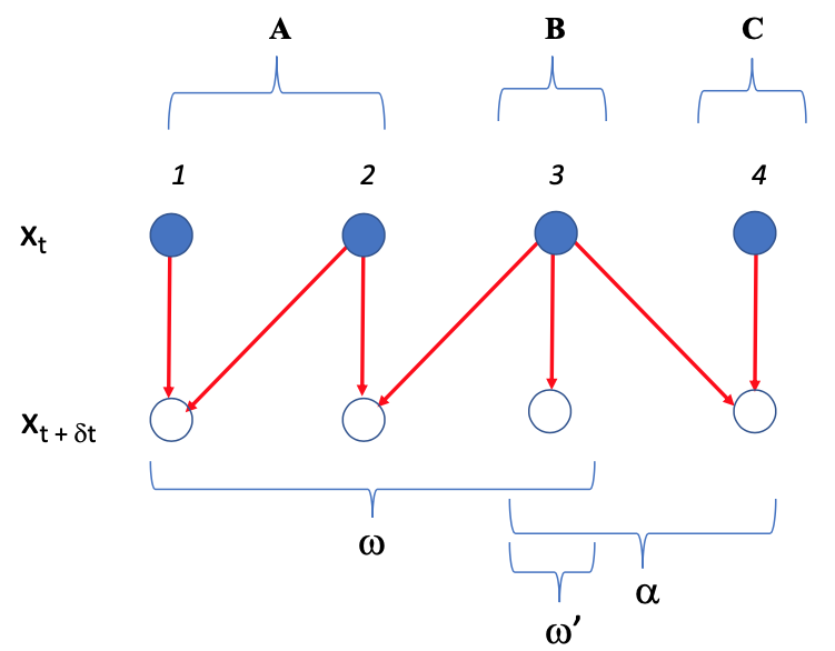
Figure 1: Four systems, $\{1,2,3,4\}$ interacting in a MPP. The red arrows indicate dependencies in the associated four rate matrices. $B$ evolves independently, but is continually observed by $A$ and $C$. So the statistical coupling between $A$ and $C$ could grow with time, even though their rate matrices do not involve one another. Three examples of units are the sets ${\omega},{\omega}^{\prime},\alpha$ indicated at the bottom: $r(1)=r(2)={\omega}$, $r(4)=\alpha$, and $r(3)={\omega}^{\prime}$.

As an example, hartich_sensory_2016 ; bo2015thermodynamic considers an MPP where receptors in a cell wall observe the concentration of a ligand in a surrounding medium, without any back-action from the receptor onto that concentration level sagawa2012fluctuation ; van2020thermodynamic ; horowitz2011designing ; shiraishi_ito_sagawa_thermo_of_time_separation.2015 ; wachtler2016stochastic ; verley_work_2014 . In addition to the medium and receptors, there is a memory that observes the state of those receptors. We can extend that scenario, to include a second set of receptors that observe the same medium (with all variables appropriately coarse-grained). Fig. 1 illustrates this MPP; system $3$ is the concentration level, system $2$ is the first set of receptors observing that concentration level, system $1$ is the memory, and system $4$ is the second set of receptors.

Taking $k_{B}=1$, I write the inverse temperature of reservoir $k$ for system $i$ as $\beta_{i}^k$, the associated chemical potentials as $\mu_{i}^k$ (with $\mu_{i}^k=0$ if $k$ is a heat bath), and any associated conserved quantities as $n_{i}^k(x_{i})$. So the rate matrix of system $i$ is $K_{x}^{x^{\prime}}(i;t)=\sum_{k}K_{x}^{x^{\prime}}(i;k,t)$. Any fluctuations of $x$ in which only $x_{i}$ changes are determined by exchanges between $i$ and its reservoirs. Moreover, since we have a MPP, the rate matrices $K(j;t)$ for $j\neq i$ must equal zero for such a fluctuation in the state of $i$. Therefore, writing $H_{x}(t)$ for the global Hamiltonian, thermodynamic consistency rao2018conservation ; van2013stochastic says that for all $i,k,t,x,x^{\prime}$,

$$\!\!\!\!\!\!\!\!\!\!\!\!\ln\dfrac{K^{x^{\prime}}_{x}(i;k,t)}{K^{x}_{x^{\prime}}(i;k,t)}=\beta_{i}^k\left(\left[H_{x^{\prime}}(t)-H_{x}(t)\right]+\mu_{i}^k\left[n_{i}^k(x_{i})-n_{i}^k(x^{\prime}_{i})\right]\right)$$ (4)

so long as both $x_{-i}=x^{\prime}_{-i}$ and $K^{x^{\prime}}_{x}(i;k,t)\neq\delta(x^{\prime}_{i},x_{i})$.

The LHS of Eq. 4 cannot depend on values $x_{j}$ or $x^{\prime}_{j}$ for $j\not\in r(i)$. Since we are only ever interested in differences in energy, this means that we must be able to rewrite the RHS of Eq. 4 as

$$\beta_{i}^k\left(\left[H_{x^{\prime}_{r(i)}}(i;t)-H_{x_{r(i)}}(i;t)\right]+\mu_{i}^k\left[n_{i}^k(x_{i})-n_{i}^k(x^{\prime}_{i})\right]\right)$$ (5)

for some local Hamiltonians $H_{x_{r(i)}}(i;t)$. (Some general thermodynamic consequences of this system LDB (SLDB) condition are discussed in the Supplemental Material at [URL will be inserted by publisher].)

To define trajectory-level quantities, first, for any set of systems $\alpha$, define the local stochastic entropy as

$$s^{\alpha}({\boldsymbol{x}}_{\alpha}(t)) :=-\ln p_{{\boldsymbol{x}}_{\alpha}(t)}(t)$$ (6)

In general I will use the prefix $\Delta$ to indicate the change of a variable’s value from $t=0$ to $t=t_{f}$, e.g.,

$$\Delta s^{\alpha}({\boldsymbol{x}}_{\alpha}) :=\ln p_{{\boldsymbol{x}}_{\alpha}(0)}(0)-\ln p_{{\boldsymbol{x}}_{\alpha}(t_{f})}(t_{f})$$ (7)

The trajectory-level entropy flows (EFs) between a system $i$ and its reservoirs along a trajectory is written as $Q^i({\boldsymbol{x}})$. The local EF into $\alpha$ is the total EF into the systems $\alpha$ from their reservoirs during $[0,t_{f}]$:

$$Q^\alpha({\boldsymbol{x}}) :=\sum_{i\in\alpha}Q^i({\boldsymbol{x}})$$ (8)

The local EP of any set of systems $\alpha$ is

$$\sigma^\alpha({\boldsymbol{x}}) :=\Delta s^\alpha({\boldsymbol{x}})-Q^\alpha({\boldsymbol{x}})$$ (9)

which can be evaluated by combining Eq. 7 and the expansion of local EF in the Supplemental Material at [URL will be inserted by publisher]. For any unit ${\omega}$, the expectation of $\sigma^{\omega}$ is non-negative. (This is not true for some quantities called “entropy production” in the literature, nor for the analogous expression “$\sigma_{x}$” defined just before Eq. (21) in shiraishi2015fluctuation .) Due to the definition of a unit, the definition of $Q^i({\boldsymbol{x}})$, and Eq. 8, the EF into (the systems in) ${\omega}$ along trajectory ${\boldsymbol{x}}$ is only a function of ${\boldsymbol{x}}_{\omega}$. So we can write $Q^{\omega}({\boldsymbol{x}})=Q^{\omega}({\boldsymbol{x}}_{\omega})$. Since $\Delta s^{\omega}({\boldsymbol{x}})$ also only depends on ${\boldsymbol{x}}_{\omega}$, we can write $\sigma^{\omega}({\boldsymbol{x}})$ as $\sigma^{\omega}({\boldsymbol{x}}_{\omega})$.

Setting $\alpha=\mathcal{N}$ in Eqs. 7 and 9 allows us to define global versions of those trajectory-level thermodynamic quantities. In particular, the global EP is

$$\sigma^\mathcal{N}({\boldsymbol{x}}) :=\Delta s^\mathcal{N}({\boldsymbol{x}})-Q^\mathcal{N}({\boldsymbol{x}})$$ (10)

There are several ways to expand the RHS of Eq. 10. One of them, discussed in the Supplemental Material at [URL will be inserted by publisher], involves an extension of what is called the “learning rate” of a bipartite process barato_efficiency_2014 ; hartich_stochastic_2014 ; hartich_sensory_2016 ; matsumoto2018role ; Brittain_2017 , to MPPs with more than two systems wolpert2020minimal . Here I focus on a different decomposition.

To begin, let ${\mathcal{N}^*}=\{{\omega}_{j}:j=1,2,\ldots,n\}$ be a dependency structure. Suppose we have a set of functions indexed by the units, $\{f^{{\omega}_{j}}:{\boldsymbol{X}}\rightarrow{\mathbb{R}}\}$. The associated inclusion-exclusion sum (or just “in-ex sum”) is defined as

$$\widehat{\sum_{{\omega}^{\prime}\in{\mathcal{N}^*}}}f^{{\omega}^{\prime}}({\boldsymbol{x}}) :=\sum_{j=1}^nf^{{\omega}_{j}}({\boldsymbol{x}})-\sum_{1\leq j<j^{\prime}\leq n}f^{{\omega}_{j}\cap{\omega}_{j^{\prime}}}({\boldsymbol{x}})$$

$$\qquad+\sum_{1\leq j<j^{\prime}<j^{\prime\prime}\leq n}f^{{\omega}_{j}\cap{\omega}_{j^{\prime}}\cap{\omega}_{j^{\prime\prime}}}({\boldsymbol{x}})-\ldots$$ (11)

The time-$t$ in-ex information is then defined as

$${\mathcal{I}}^{\mathcal{N}^*}({\boldsymbol{x}}(t)):=\left[\widehat{\sum_{{\omega}\in{\mathcal{N}^*}}}s^{\omega}({\boldsymbol{x}}(t))\right]-s({\boldsymbol{x}}(t))$$ (12)

(A related concept, not involving a dependency structure, is called “co-information” in bell2003co .) As an example, if ${\mathcal{N}^*}$ consists of two units, ${\omega}_{1},{\omega}_{2}$, with no intersection, then the expected in-ex information at time $t$ is just the mutual information between those units at that time. More generally, if there an arbitrary number of units in ${\mathcal{N}^*}$ but none of them overlap, then the expected in-ex information is the “total correlation” ting1962amount ; wolpert2020minimal ,

$$I\left(X^{{\omega}_{1}}(t);X^{{\omega}_{2}}(t);\ldots\right) :=\left(\sum_{\omega}\langle s^{\omega}(t)\rangle\right)-\langle s(t)\rangle$$ (13)

Since dependency structures are closed under intersections, if we apply the inclusion-exclusion principle to the expressions for local and global EF we get

$$Q({\boldsymbol{x}}) =\widehat{\sum_{{\omega}\in{\mathcal{N}^*}}}{Q}^{\omega}({\boldsymbol{x}})$$ (14)

Combining this with Eqs. 7, 9, 10 and 12 gives

$$\sigma^\mathcal{N}({\boldsymbol{x}}) =\widehat{\sum_{{\omega}\in{\mathcal{N}^*}}}\sigma^{{\omega}}({\boldsymbol{x}})-\Delta{\mathcal{I}}^{{\mathcal{N}^*}}({\boldsymbol{x}})$$ (15)

Taking expectations of both sides of Eq. 15 we get

$$\langle\sigma^\mathcal{N}\rangle =\widehat{\sum_{{\omega}\in{\mathcal{N}^*}}}\langle\sigma^{{\omega}}\rangle-\langle\Delta{\mathcal{I}}^{{\mathcal{N}^*}}\rangle$$ (16)

As a simple example, if there are no overlaps between any units, then expected global EP reduces to

$$\langle\sigma^\mathcal{N}\rangle =\sum_{\omega}\langle\sigma^{\omega}\rangle-\langle\Delta I\left(X^{{\omega}_{1}};X^{{\omega}_{2}};\ldots\right)\rangle$$ (17)

$$\geq-\langle\Delta I\left(X^{{\omega}_{1}};X^{{\omega}_{2}};\ldots\right)\rangle$$ (18)

which is a strengthened second law of thermodynamics.

Multipartite Fluctuation Theorems.— Write $\tilde{{\boldsymbol{x}}}$ for ${\boldsymbol{x}}$ reversed in time, i.e., $\tilde{{\boldsymbol{x}}}(t)={\boldsymbol{x}}(t_{f}-t)$. Write ${\mathbb{P}}({\boldsymbol{x}})$ for the probability density function over trajectories generated by starting from the initial distribution $p_{x}(0)$, and write $\tilde{{\mathbb{P}}}({\boldsymbol{x}})$ for the probability density function over trajectories generated by starting from the ending distribution $p_{x}(t_{f})$, and then evolving according to the time-reversed sequence of rate matrices, $\tilde{K}(t)=K(t_{f}-t)$.

Let ${\mathcal{A}}$ be any set of units (not necessarily a dependency structure) and write $\sigma^{{\mathcal{A}}}({\boldsymbol{x}})$ for the total EP generated by the systems in ${\mathcal{A}}$ under ${\mathbb{P}}$. (Note that since $\cup{\mathcal{A}}$ is a union of units, we can write $\sigma^{{\mathcal{A}}}({\boldsymbol{x}})$ as $\sigma^{{\mathcal{A}}}({\boldsymbol{x}}_{\mathcal{A}})$.) Define $\vec{\sigma}^{\mathcal{A}}$ as the vector whose components are the local EP values $\sigma^\alpha$ for all $\alpha\in{\mathcal{A}}$ (including $\alpha={\mathcal{A}}$). One can prove the associated detailed fluctuation theorem (DFT)

$$\ln\left[\dfrac{{\mathbb{P}}(\vec{\sigma}^{\mathcal{A}})}{\tilde{{\mathbb{P}}}(-\vec{\sigma}^{\mathcal{A}})}\right] =\sigma^{{\mathcal{A}}}$$ (19)

where $\tilde{{\mathbb{P}}}(-\vec{\sigma}^{\mathcal{A}})$ is the joint probability of the specified vector of EP values under ${\tilde{{\mathbb{P}}}}$.

Subtracting instances of Eq. 19 evaluated for different choices of ${\mathcal{A}}$ gives conditional DFTs, which in turn give conditional integral fluctuation theorems (IFTs). As an example, subtract Eq. 19 for ${\mathcal{A}}$ set to some singleton $\{{\omega}\}$ from Eq. 19 for ${\mathcal{A}}=\mathcal{N}$. This gives

$$\left\langle e^{\sigma^{\omega}-\sigma^\mathcal{N}}\,|\,\sigma^{\omega}\right\rangle =1$$ (20)

(for any specific EP value $\sigma^{\omega}$ such that both ${\mathbb{P}}(\sigma^{\omega})$ and $\tilde{{\mathbb{P}}}(-\sigma^{\omega})$ are nonzero). Jensen’s inequality then gives $\left\langle\sigma^\mathcal{N}\,|\,\sigma^{\omega}\right\rangle\geq\sigma^{\omega}$ and so averaging over $\sigma^{\omega}$,

$$\left\langle\sigma^\mathcal{N}\right\rangle\geq\left\langle\sigma^{\omega}\right\rangle$$ (21)

Plugging in Eq. 15 then gives

$${\widehat{\sum}}_{{\omega}^{\prime}\in{\mathcal{N}^*}}\langle\sigma^{{\omega}^{\prime}}\rangle-\langle\Delta{\mathcal{I}}^{{\mathcal{N}^*}}\rangle\geq\langle\sigma^{{\omega}}\rangle$$ (22)

The multi-divergence for a set of units ${\mathcal{A}}$ is

$$D\left({\mathbb{P}}(\vec{\sigma}^{\mathcal{A}})\;||\;\tilde{{\mathbb{P}}}(-\vec{\sigma}^{\mathcal{A}})\right)-\sum_{{\mathcal{A}}_{i}\in{\mathcal{A}}}D\left({\mathbb{P}}({\sigma}^{{\mathcal{A}}_{i}})\;||\;\tilde{{\mathbb{P}}}(-\sigma^{{\mathcal{A}}}_{i})\right)$$ (23)

and written as $I\left({\mathbb{P}}(\vec{\sigma}^{\mathcal{A}})\;||\;\tilde{{\mathbb{P}}}(-\vec{\sigma}^{\mathcal{A}})\right)$ wolpert_thermo_comp_review_2019 . It is an extension of the concept of the total correlation of the systems in ${\mathcal{A}}$, replacing entropies with relative entropies between forward and backward trajectories. One can prove that

$$\left\langle\sigma^\mathcal{N}\right\rangle \geq\sum_{i=1}^m\left\langle\sigma^{{\mathcal{A}}_{i}}\right\rangle+I\left({\mathbb{P}}(\vec{\sigma}^{\mathcal{A}})\;||\;\tilde{{\mathbb{P}}}(-\vec{\sigma}^{\mathcal{A}})\right)$$ (24)

with equality if $\cup_{i}{\mathcal{A}}=\mathcal{N}$. Note that the sum of local EPs in Eq. 24 is a normal sum, not an in-ex sum.

Often one can show that multi-divergence is non-negative, and so $\left\langle\sigma^\mathcal{N}\right\rangle\geq\sum_{i=1}^m\left\langle\sigma^{{\mathcal{A}}_{i}}\right\rangle$. As an example, multi-divergence reduces to total correlation (and so is non-negative) if $\tilde{{\mathbb{P}}}(-\vec{\sigma}^{\mathcal{A}})$ is a product distribution. Moreover, often $\tilde{{\mathbb{P}}}(-\vec{\sigma}^{\mathcal{A}})$ is close to being a product distribution in a relaxation process (see Supplemental Material at [URL will be inserted by publisher]).

Extended TURs and strengthened second law.— The simplified ligand-sensing example in Fig. 2 can be used to illustrate the consequences of these results. To begin, evaluate Eq. 22 for this example first for ${\omega}=AB$ and then for ${\omega}=BC$, to get

$$\min\left[\left\langle\sigma^{BC}\right\rangle,\left\langle\sigma^{AB}\right\rangle\right]-\left\langle\sigma^B\right\rangle\geq\Delta I(A;C\,|\,B)$$ (25)

where $I\left(A;C\,|\,B\right)(t)$ is the conditional mutual information at time $t$ between $x_{A}$ and $x_{C}$, given $x_{B}$. Eq. 25 is a new type of speed limit theorem: If one wants the process to (change the distributions in order to) have large $\Delta I(A;C\,|\,B)$, one must pay for it with large value of both $\left\langle\sigma^{AB}\right\rangle$ and $\left\langle\sigma^{BC}\right\rangle$. (Special cases of this kind of speed limit were implicit in some of the results in wolpert_thermo_comp_review_2019 ; wolpert_kolchinsk_first_circuits_published.2020 ; wolpert.thermo.bayes.nets.2020 .)

Next, suppose $x_{B}$ is constant during the process. Then

$$\left\langle\sigma^\mathcal{N}\right\rangle=\left\langle\sigma^{AB}\right\rangle+\left\langle\sigma^{BC}\right\rangle-\Delta I(A;C\,|\,B)\geq-\Delta I(A;C\,|\,B)$$ (26)

by Eq. 15. One can prove that $\Delta I(A;C\,|\,B)\leq 0$ if $x_{B}$ is constant. So when the ligand concentration in the medium is constant (to within the precision of the coarse-grained binning of $X_{B}$), Eq. 26 is stronger than the conventional second law (see Fig. 2(b)).

Now suppose only that system $B$ is subject to a TUR, e.g., it’s in an NESS, so that $\langle\sigma^B\rangle\geq 2\langle J_{B}\rangle^2/{\mbox{Var}}(J_{B})$, where $J_{B}({\boldsymbol{x}}_{B})$ is an arbitrary current among $B$’s states (see Fig. 2(c)). Plugging this into Eq. 25, applying Eq. 21 for ${\omega}=BC$, and then applying Eq. 21 for ${\omega}=B$, we derive a new kind of TUR:

$$\langle\sigma^\mathcal{N}\rangle\geq 2\langle J_{B}\rangle^2/{\mbox{Var}}(J_{B})+\max\left[\Delta I(A;C\,|\,B),0\right]$$ (27)

Next, choose ${\mathcal{A}}=\{AB,BC\}$ in Eq. 24 to get

$$\left\langle\sigma^\mathcal{N}\right\rangle\geq\left\langle\sigma^{AB}\right\rangle+\left\langle\sigma^{BC}\right\rangle+I\left({\mathbb{P}}(\sigma^{AB},\sigma^{BC})\;||\;\tilde{{\mathbb{P}}}(-\sigma^{AB},-\sigma^{BC})\right)$$ (28)

One can prove that for broad classes of MPPs, $I\left({\mathbb{P}}(\sigma^{AB},\sigma^{BC})\;||\;\tilde{{\mathbb{P}}}(-\sigma^{AB},-\sigma^{BC})\right)\geq 0$. In particular this holds if the rate matrices are time-homogeneous, the Hamiltonian is uniform and unchanging, and $B$ relaxes to its equilibrium distribution by time $t_{f}$. In this scenario the relaxing unit $BC$ obeys the conditions for the arbitrary initial state TUR liu2020thermodynamic . Suppose as well that $AB$ obeys the conditions for the NESS-based TUR (see Fig. 2(d)). Then Eq. 28 lower bounds expected global EP in terms of current precisions in different units:

$$\langle\sigma^\mathcal{N}\rangle \geq 2\dfrac{\langle J_{AB}\rangle^2}{{\mbox{Var}}(J_{AB})}+\dfrac{\langle t_{f}j_{BC}(t_{f})\rangle^2}{{\mbox{Var}}(J_{BC})}$$ (29)

($j_{BC}(t_{f})$ is the derivative of the expectation of an arbitrary current in joint system $BC$, evaluated at $t_{f}$). Importantly, Eqs. 27 and 29 hold even if the full system does not satisfy conditions for any conventional TUR.

Finally, combining Eqs. 28 and 16 gives

$$\left\langle\sigma^B\right\rangle\leq-\Delta I(A;C\,|\,B)-I\left({\mathbb{P}}(\sigma^{AB},\sigma^{BC})\;||\;\tilde{{\mathbb{P}}}(-\sigma^{AB},-\sigma^{BC})\right)$$ (30)

When $I\left({\mathbb{P}}(\sigma^{AB},\sigma^{BC})\;||\;\tilde{{\mathbb{P}}}(-\sigma^{AB},-\sigma^{BC})\right)\geq 0$ (e.g., in Fig. 2(d)), Eq. 30 upper-bounds EP in the intercellular medium in terms of a purely information-theoretic quantity, $-\Delta I(A;C\,|\,B)$, which also involves the cell wall receptor systems $A$ and $C$. (Eq. 30 also shows that it is impossible to have both $\Delta I(A;C\,|\,B)>0$ and $I\left({\mathbb{P}}(\sigma^{AB},\sigma^{BC})\;||\;\tilde{{\mathbb{P}}}(-\sigma^{AB},-\sigma^{BC})\right)>0$.)

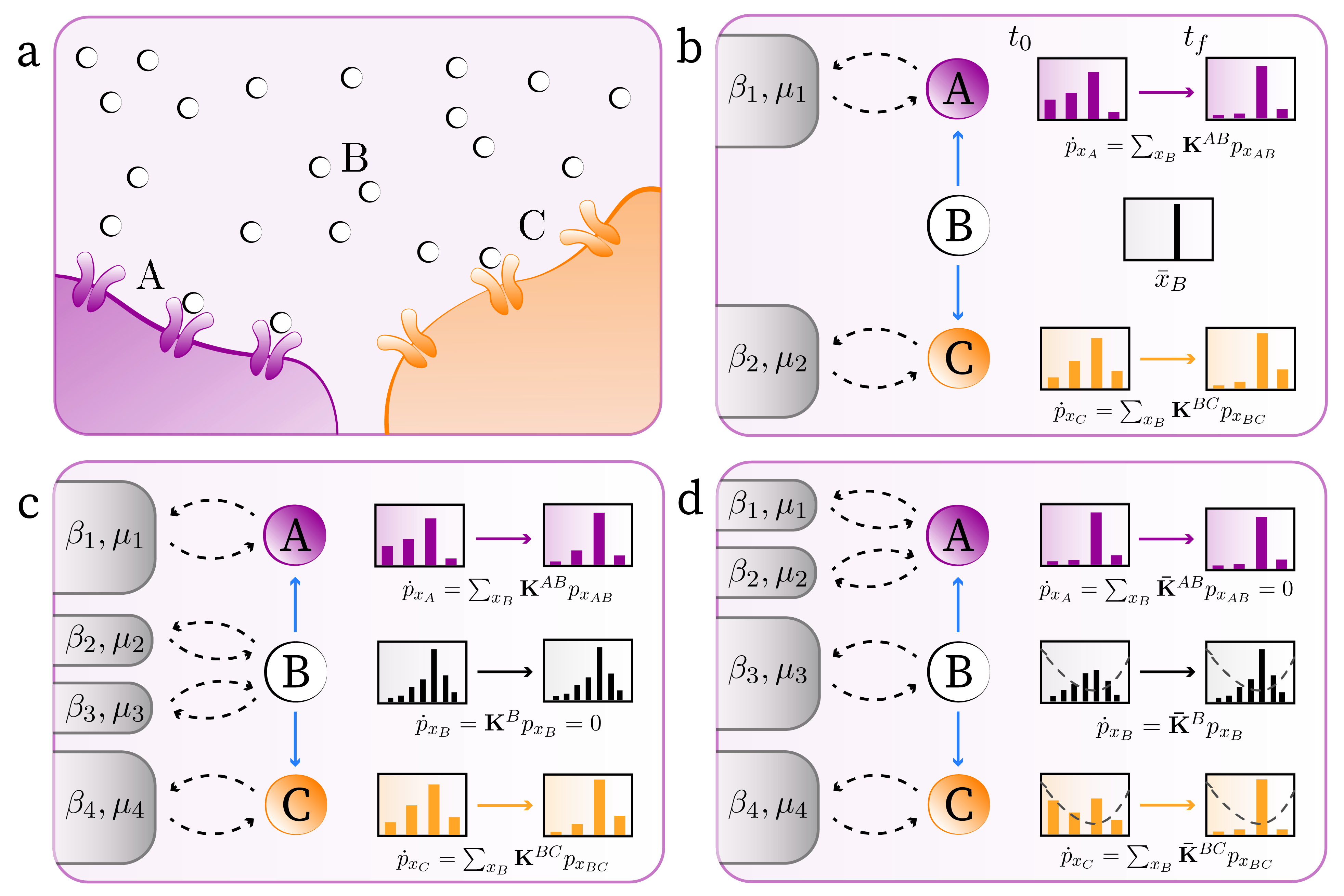
Figure 2: (a) The MPP discussed in the text. The state of the intercellular medium (system $B$) is the (discretized) concentration of a ligand and the states of the cell-wall receptors (systems $A,C$) are their respective observations of that concentration. (b) In this scenario system $B$ does not change its state. (Histograms indicate starting and ending distributions.) (c) In this scenario system $B$ is in an NESS. (d) In this scenario joint system $AB$ is in an NESS. (Overbars indicate time-homogeneous rate matrices.)

Discussion.— In many sets of co-evolving systems, the times of each system’s state transitions is random. In this paper I derive FTs that govern such sets of systems. I then use those FTs to derive a strengthened second law, and to substantially extend all currently known TURs: even if the overall system does not meet any criteria for a TUR, the expected EP of the overall system is lower-bounded by the current precisions of any of the constituent systems that separately meet such criteria.

Acknowledgements.— I thank Farita Tasnim, Gülce Kardes, and Artemy Kolchinsky for helpful discussion. This work was supported by the Santa Fe Institute, US NSF Grant CHE-1648973 and FQXi Grant FQXi-RFP-IPW-1912.

Appendix A Entropy flow into systems and units

To fully define the entropy flow into systems we need to introduce some more notation. Let $M({\boldsymbol{x}})$ be the total number of state transitions during the time interval $[0,t_{f}]$ by all systems (which might equal $0$). If $M({\boldsymbol{x}})\geq 1$, define $\eta_{\boldsymbol{x}}:\{1,\ldots,M({\boldsymbol{x}})\}\rightarrow\mathcal{N}$ as the function that maps any integer $j\in\{1,\ldots,M({\boldsymbol{x}})\}$ to the system that changes its state in the $j$’th transition. Let $k(j)$ be the associated function specifying which reservoir is involved in that $j$’th transition. (So for all $j$, $k(j)$ specifies a reservoir of system $\eta(j)$.) Similarly, let $\tau_{\boldsymbol{x}}:\{0,\ldots,M({\boldsymbol{x}})\}\rightarrow\mathcal{N}$ be the function that maps any integer $j\in\{1,\ldots,M({\boldsymbol{x}})\}$ to the time of the $j$’th transition, and maps $0$ to the time $0$.

From now on, I leave the subscript ${\boldsymbol{x}}$ on the maps $\eta_{\boldsymbol{x}}$ and $\tau_{\boldsymbol{x}}$ implicit. So for example, $\eta^{-1}(i)$ is the set (of indices specifying) all state transitions at which system $i$ changes state in the trajectory ${\boldsymbol{x}}$. More generally, for any set of systems $\alpha$, $\eta^{-1}(\alpha):=\cup_{i\in\alpha}\eta^{-1}(i)$ is the set of all state transitions at which a system $i\in\alpha$ changes state in the trajectory ${\boldsymbol{x}}$.

Given these definitions, the total entropy flow into system $i$ from its reservoirs during $[0,t_{f}]$ is

$$Q^i({\boldsymbol{x}}) :=\sum_{j\in\eta^{-1}(i)}\beta_{i}^{k(j)}\bigg{(}H_{{{\boldsymbol{x}}}_{r(i)}(\tau(j))}(i;\tau(j))-H_{{{\boldsymbol{x}}}_{r(i)}(\tau(j-1))}(i;\tau(j))$$

$$\qquad+\mu_{i}^{k(j)}\left[n_{i}^{k(j)}({{\boldsymbol{x}}}_{i}(\tau(j-1))-n_{i}^{k(j)}({{\boldsymbol{x}}}_{i}(\tau(j))\right]\bigg{)}$$ (31)

where I interpret the sum on the RHS to be zero if system $i$ never undergoes a state transition in trajectory ${\boldsymbol{x}}$. As mentioned in the text, the local EF into a unit $\alpha$ for trajectory ${\boldsymbol{x}}$ is just the sum of the EFs into all the systems in $\alpha$ for that trajectory.

Expanding, under Eq. 5,

$$Q^\alpha({\boldsymbol{x}}) =\sum_{i\in\alpha}\sum_{j\in\eta^{-1}(i)}\ln\left[\dfrac{K^{{{\boldsymbol{x}}}_{r(i)}(\tau(j))}_{{{\boldsymbol{x}}}_{r(i)}(\tau(j-1))}(i;k(j),\tau(j))}{K^{{{\boldsymbol{x}}}_{r(i)}(\tau(j-1))}_{{{\boldsymbol{x}}}_{r(i)}(\tau(j))}(i;k(j),\tau(j))}\right]$$ (32)

So in the special case that $\alpha$ is a unit,

$$Q^\alpha({\boldsymbol{x}}) =\sum_{i\in\alpha}\sum_{j\in\eta^{-1}(i)}\ln\left[\dfrac{K^{{{\boldsymbol{x}}}_{\alpha}(\tau(j))}_{{{\boldsymbol{x}}}_{\alpha}(\tau(j-1))}(i;k(j),\tau(j))}{K^{{{\boldsymbol{x}}}_{\alpha}(\tau(j-1))}_{{{\boldsymbol{x}}}_{\alpha}(\tau(j))}(i;k(j),\tau(j))}\right]$$ (33)

Note that ${{\boldsymbol{x}}}_{-i}(\tau(j-1))={{\boldsymbol{x}}}_{-i}(\tau(j))$ for all systems $i$, for all $j\in\eta^{-1}(i)$, since the process is multipartite. Therefore the global EF can be written as

$$Q({\boldsymbol{x}})=\sum_{i}Q^i({\boldsymbol{x}})=\sum_{j=1}^{M({\boldsymbol{x}})}\ln\left[\dfrac{K^{{{\boldsymbol{x}}}(\tau(j))}_{{{\boldsymbol{x}}}(\tau(j-1))}(\tau(j))}{K^{{{\boldsymbol{x}}}(\tau(j-1))}_{{{\boldsymbol{x}}}(\tau(j))}(\tau(j))}\right]$$ (34)

As a final, technical point, note that ${\boldsymbol{x}}$ is fully specified by $M,\tau,k,\eta$ and the finite list of the precise state transitions at the times listed in $\tau$ by the associated systems listed in $\eta$ mediated by the associated reservoirs listed in $k$. So the probability measure of a trajectory ${\boldsymbol{x}}$ is

$${\mathbb{P}}({\boldsymbol{x}})=P(M)P({\boldsymbol{x}}\,|\,M,\tau,k,\eta)P(\tau,k,\eta\,|\,M)$$ (35)

For each integer $M$, all the terms on the RHS are either probability distributions or probability density functions, and therefore we can define the integral over $M,\tau,k,\eta,{\boldsymbol{x}}$. So in particular, $\delta$ function over trajectories in the equations in the main text is shorthand for a function that equals zero everywhere that its argument is nonzero, and such that its integral equals $1$.

Appendix B Example where global Hamiltonian cannot equal sum of local Hamiltonians under SLDB

The global Hamiltonian need not be a sum of the local Hamiltonians. Indeed, it’s possible that all local Hamiltonians equal one another and also equal the global Hamiltonian. To see this, consider a scenario where there are exactly two distinct systems $i,j$, which both observe one another very closely, so that the rate matrices of both of them have approximately as much dependence on the state of the other system as on their own state. In this scenario, there is a single unit, $r(i)=r(j)=\{i,j\}=\mathcal{N}$. Assume as well that each system is only connected to a single heat bath, with no other reservoirs.

If we took the global Hamiltonian to be $H_{x}(t)=H_{x}(i;t)+H_{x}(j;t)$, its change under the fluctuation $(x^{\prime}_{i},x_{j})\rightarrow(x_{i},x_{j})$ would be

$$H_{x_{i},x_{j}}(i;t)-H_{x^{\prime}_{i},x_{j}}(i;t)+H_{x_{i},x_{j}}(j;t)-H_{x^{\prime}_{i},x_{j}}(j;t)$$ (36)

This is the change in energy of the total system during the transition. Moreover, since this state transition only changes the state of system $i$ and since we assume the dynamics is a MPP, only the heat bath of system $i$ could have changed its energy during the transition. Therefore by conservation of energy, the change in the energy of the bath of system $i$ must equal the expression in Eq. 36.

Under SLDB, that change in the energy of the heat bath of system $i$ would be the change in the local Hamiltonian of system $i$. Therefore to have SLDB be even approximately true, it would have to be the case that

$$|H_{x_{i},x_{j}}(i;t)-H_{x^{\prime}_{i},x_{j}}(i;t)|\; \gg\;|H_{x_{i},x_{j}}(j;t)-H_{x^{\prime}_{i},x_{j}}(j;t)|$$ (37)

for all pairs $x,x^{\prime}$. Similarly, to address the case where a fluctuation to $x_{j}$ arises due to $j$’s interaction with its heat bath, we would need to have

$$|H_{x_{i},x_{j}}(j;t)-H_{x_{i},x^{\prime}_{j}}(j;t)|\; \gg\;|H_{x_{j},x_{j}}(i;t)-H_{x_{i},x^{\prime}_{j}}(i;t)|$$ (38)

for all pairs $x,x^{\prime}$.

Next, we need to formalize our requirement that “the rate matrices of both {systems} have approximately as much dependence on the state of the other system as on their own state”. One way to do that is to require that the dependence on $x_{j}$ of (the ratio of forward and backward terms in) $i$’s rate matrix is not much smaller than the typical terms in that rate matrix, i.e., for all pairs $x,x^{\prime}$,

$$\left|\left(H_{x_{i},x_{j}}(i;t)-H_{x^{\prime}_{i},x_{j}}(i;t)\right)-\left(H_{x_{i},x^{\prime}_{j}}(i;t)-H_{x^{\prime}_{i},x^{\prime}_{j}}(i;t)\right)\right|$$

$$\qquad\mathrel{\overset{\;}{\scalebox{1.5}[1.0]{$\sim$}}}\dfrac{\left|H_{x_{i},x_{j}}(i;t)-H_{x^{\prime}_{i},x_{j}}(i;t)\right|+\left|H_{x_{i},x^{\prime}_{j}}(i;t)-H_{x^{\prime}_{i},x^{\prime}_{j}}(i;t)\right|}{2}$$

$$\qquad:=\Delta_{i;x,x^{\prime}}$$ (39)

Similarly, since system $j$ is also observing $i$,

$$\left|\left(H_{x_{i},x_{j}}(j;t)-H_{x_{i},x^{\prime}_{j}}(j;t)\right)-\left(H_{x^{\prime}_{i},x_{j}}(j;t)-H_{x^{\prime}_{i},x^{\prime}_{j}}(j;t)\right)\right|$$

$$\qquad\mathrel{\overset{\;}{\scalebox{1.5}[1.0]{$\sim$}}}\dfrac{\left|\left(H_{x_{i},x_{j}}(j;t)-H_{x_{i},x^{\prime}_{j}}(j;t)\right)+\left(H_{x^{\prime}_{i},x_{j}}(j;t)-H_{x^{\prime}_{i},x^{\prime}_{j}}(j;t)\right)\right|}{2}$$

$$\qquad:=\Delta_{j;x,x^{\prime}}$$ (40)

Plugging Eq. 37 into the definition of $\Delta_{i;x,x^{\prime}}$ and then using the fact that for any real numbers $a,b$, $|a-b|<|a|+|b|$, we get

$$\left|\left(H_{x_{i},x_{j}}(j;t)-H_{x^{\prime}_{i},x_{j}}(j;t)\right)-\left(H_{x_{i},x^{\prime}_{j}}(j;t)-H_{x^{\prime}_{i},x^{\prime}_{j}}(j;t)\right)\right|$$

$$\qquad\ll\Delta_{i;x,x^{\prime}}$$ (41)

In addition, shuffling terms in the LHS of Eq. 39 gives

$$\left|\left(H_{x_{i},x_{j}}(i;t)-H_{x_{i},x^{\prime}_{j}}(i;t)\right)-\left(H_{x^{\prime}_{i},x_{j}}(i;t)-H_{x^{\prime}_{i},x^{\prime}_{j}}(i;t)\right)\right|$$

$$\qquad\mathrel{\overset{\;}{\scalebox{1.5}[1.0]{$\sim$}}}\Delta_{i;x,x^{\prime}}$$ (42)

The analogous reasoning with Eqs. 38 and 40 gives

$$\left|\left(H_{x_{i},x^{\prime}_{j}}(i;t)-H_{x_{i},x_{j}}(i;t)\right)-\left(H_{x^{\prime}_{i},x^{\prime}_{j}}(i;t)-H_{x^{\prime}_{i},x_{j}}(i;t)\right)\right|$$

$$\qquad\ll\Delta_{j;x,x^{\prime}}$$ (43)

and

$$\left|\left(H_{x_{i},x_{j}}(j;t)-H_{x^{\prime}_{i},x_{j}}(j;t)\right)-\left(H_{x_{i},x^{\prime}_{j}}(j;t)-H_{x^{\prime}_{i},x^{\prime}_{j}}(j;t)\right)\right|$$

$$\qquad\mathrel{\overset{\;}{\scalebox{1.5}[1.0]{$\sim$}}}\Delta_{j;x,x^{\prime}}$$ (44)

Comparing Eqs. 42 and 43 establishes that $\Delta_{i;x,x^{\prime}}\ll\Delta_{j;x,x^{\prime}}$. However, comparing Eqs. 41 and 44 establishes that $\Delta_{j;x,x^{\prime}}\ll\Delta_{i;x,x^{\prime}}$. This contradiction shows that it is not possible for the global Hamiltonian to be a sum of the two local Hamiltonians, given that both systems “observe one another very closely”. (See Appendix G.)

Appendix C Alternative expansion of trajectory-level global EP

C.1 Definition of $\chi^{\omega}({\boldsymbol{x}})$

First, for any unit ${\omega}$, define

$$\chi^{\omega}({\boldsymbol{x}}):=\sigma^\mathcal{N}({\boldsymbol{x}})-\sigma^{\omega}({\boldsymbol{x}})$$ (45)

I now show that

$$\chi^{\omega}({\boldsymbol{x}}) =\Delta s^{-{\omega}\,|\,{\omega}}({\boldsymbol{x}})-Q^{-{\omega}}({\boldsymbol{x}})$$ (46)

where

$$\Delta s^{-{\omega}\,|\,{\omega}}({\boldsymbol{x}}) =\Delta s^{-{\omega},{\omega}}({\boldsymbol{x}})-\Delta s^{{\omega}}({\boldsymbol{x}})$$ (47)

$$=-\Delta\ln p_{{\omega},-{\omega}}({\boldsymbol{x}})+\Delta\ln p_{{\omega}}({\boldsymbol{x}})$$ (48)

$$=-\Delta\ln p_{\mathcal{N}}({\boldsymbol{x}})+\Delta\ln p_{{\omega}}({\boldsymbol{x}})$$ (49)

is the change in the value of the conditional stochastic entropy of the entire system given the state of ${\omega}$. Note that in general $-{\omega}$ will not be a unit. So the entropy flow into the associated reservoirs, $Q^{-{\omega}}({\boldsymbol{x}})$, may depend on the trajectory of systems outside of $-{\omega}$, i.e., it may depend on ${\boldsymbol{x}}_{{\omega}}$.

As shorthand, from now on I leave the function $\tau$ implicit, so that for example, ${\boldsymbol{x}}(\tau(j))$ gets shortened to ${\boldsymbol{x}}(j)$. (Note though that with slight abuse of notation, I still take ${\boldsymbol{x}}(t_{f})$ to mean the state of the system at $t=t_{f}$ under trajectory ${\boldsymbol{x}}$.) Given any unit ${\omega}$, we can expand the global EP as

$$\sigma^\mathcal{N}({\boldsymbol{x}}) =\ln p_{{\boldsymbol{x}}(0)}(0)-\ln p_{{\boldsymbol{x}}(t_{f})}(t_{f})+\sum_{j=1}^{M({\boldsymbol{x}})}\ln\left[\dfrac{K^{{{\boldsymbol{x}}}(j-1)}_{{{\boldsymbol{x}}}(j)}(\eta(j);j)}{K^{{{\boldsymbol{x}}}(j)}_{{{\boldsymbol{x}}}(j-1)}(\eta(j);j)}\right]$$

$$=\ln p^{X_{\omega}}_{{\boldsymbol{x}}_{\omega}(0)}(0))-\ln p^{X_{\omega}}_{{\boldsymbol{x}}_{\omega}(t_{f})}(t_{f})+\sum_{j\in\eta^{-1}({\omega})}\ln\left[\dfrac{K^{{{\boldsymbol{x}}_{\omega}}(j-1)}_{{{\boldsymbol{x}}_{\omega}}(j)}(\eta(j);j)}{K^{{{\boldsymbol{x}}}_{\omega}(j)}_{{{\boldsymbol{x}}_{\omega}}(j-1)}(\eta(j);j)}\right]$$

$$\qquad\qquad+\ln p^{X|X_{\omega}}_{{\boldsymbol{x}}(0)}(0)-\ln p^{X|X_{\omega}}_{{\boldsymbol{x}}(t_{f})}(t_{f})+\sum_{j\in\eta^{-1}(-{\omega})}\ln\left[\dfrac{K^{{{\boldsymbol{x}}}(j-1)}_{{{\boldsymbol{x}}}(j)}(\eta(j);j)}{K^{{{\boldsymbol{x}}}(j)}_{{{\boldsymbol{x}}}(j-1)}(\eta(j);j)}\right]$$

$$=\sigma^{\omega}({\boldsymbol{x}})+\ln p^{X|X_{\omega}}_{{\boldsymbol{x}}(0)}(0)-\ln p^{X|X_{\omega}}_{{\boldsymbol{x}}(t_{f})}(t_{f})+\sum_{j\in\eta^{-1}(-{\omega})}\ln\left[\dfrac{K^{{{\boldsymbol{x}}}(j-1)}_{{{\boldsymbol{x}}}(j)}(\eta(j);j)}{K^{{{\boldsymbol{x}}}(j)}_{{{\boldsymbol{x}}}(j-1)}(\eta(j);j)}\right]$$ (50)

Expand

$$\Delta s^{{-{\omega}}|{\omega}}({\boldsymbol{x}}) =\Delta s^{(-{\omega},{\omega})\,|\,{\omega}}({\boldsymbol{x}})$$ (51)

$$=\Delta s^{\mathcal{N}\,|\,{\omega}}({\boldsymbol{x}})$$ (52)

$$=\ln p^{\mathcal{N}|{\omega}}_{{\boldsymbol{x}}(0)}(0)-\ln p^{\mathcal{N}|{\omega}}_{{\boldsymbol{x}}(t_{f})}(t_{f})$$ (53)

This allows us to rewrite Eq. 50 more succinctly as

$$\chi^{\omega}({\boldsymbol{x}}) =\Delta s^{\mathcal{N}\,|\,{\omega}}({\boldsymbol{x}})+\sum_{j\in\eta^{-1}(-{\omega})}\ln\left[\dfrac{K^{{{\boldsymbol{x}}}(j-1)}_{{{\boldsymbol{x}}}(j)}(\eta(j);j)}{K^{{{\boldsymbol{x}}}(j)}_{{{\boldsymbol{x}}}(j-1)}(\eta(j);j)}\right]$$

$$=\Delta s^{\mathcal{N}\,|\,{\omega}}({\boldsymbol{x}})-Q^{-{\omega}}({\boldsymbol{x}})$$ (54)

which establishes Eq. 46.

C.2 FTs involving $\chi^{\omega}({\boldsymbol{x}})$

To gain insight into Eq. 54, define the counterfactual rate matrix $\underline{K}(t):=K(-{\omega};t)$, and let $\underline{{\mathbb{P}}}$ be what the density over trajectories ${\boldsymbol{x}}$ would have been if the system had evolved from the initial distribution $p_{x}(0)$ under $\underline{K}(t)$ rather than $K(t)$. Define $\Delta s^{{-{\omega}}}_{\underline{{\mathbb{P}}}}({\boldsymbol{x}})$ and $\sigma_{\underline{{\mathbb{P}}}}({\boldsymbol{x}})$ accordingly. Then we can expand the second term on the RHS of Eq. 54 as

$$Q^{-{\omega}}({\boldsymbol{x}}) =\sigma_{\underline{{\mathbb{P}}}}({\boldsymbol{x}})-\Delta s^{{-{\omega}}}_{\underline{{\mathbb{P}}}}({\boldsymbol{x}})$$ (55)

So the heat flow from the baths connected to $-{\omega}$ into the associated systems is the difference between a (counterfactual) global EP and a (counterfactual) change in the entropy of those systems.

We can iterate these results, to get more refined decompositions of global EP. For example, let $\underline{\mathcal{N}}^*$ be a dependency structure of $\underline{K}$, the counterfactual rate matrix defined just before Eq. 55. Let ${\omega}$ be a unit in ${\mathcal{N}^*}$ while $\alpha$ is a unit in $\underline{\mathcal{N}}^*$. Then we can insert Eq. 55 into Eq. 46 and apply that Eq. 46 again, to the resulting term $\sigma_{\underline{{\mathbb{P}}}}$, to get

$$\sigma^\mathcal{N}({\boldsymbol{x}}) =\sigma^{\omega}({\boldsymbol{x}})+\left[\sigma^\alpha_{\underline{{\mathbb{P}}}}({\boldsymbol{x}})+\chi^{\alpha}_{\underline{{\mathbb{P}}}}({\boldsymbol{x}})+\Delta s^{\mathcal{N}\,|\,{\omega}}_{\mathbb{P}}({\boldsymbol{x}})-\Delta s^{{-{\omega}}}_{\underline{{\mathbb{P}}}}({\boldsymbol{x}})\right]$$ (56)

Note that in general, $\alpha$ might contain systems outside of $\mathcal{N}\setminus{\omega}$. As a result, it need not be a unit of the full rate matrix $K$. In addition, both (counterfactual) rates $d\left\langle\sigma^\alpha_{\underline{{\mathbb{P}}}}\right\rangle_{\underline{{\mathbb{P}}}}/dt$ and $d\left\langle\chi^\alpha_{\underline{{\mathbb{P}}}}\right\rangle_{\underline{{\mathbb{P}}}}/dt$ are non-negative. However, if we evaluate those two rates under the actual density ${\mathbb{P}}$ rather than the counterfactual $\underline{{\mathbb{P}}}$, it may be that one or the other of them is negative. This is just like how the expected values of the analogous “EP” terms in ito2013information ; shiraishi2015fluctuation , which concern a single system, may have negative derivatives.

The trajectory-level decomposition of global EP in terms of $\chi^{\omega}$ can be exploited to get other FTs in addition to those presented in the main text. For example, if we plug Eq. 45 into Eq. 28 instead of plugging in Eq. 15, and then use Eq. 46, we get

$$\left\langle e^{-\chi^{\omega}}\,|\,\sigma^{\omega}\right\rangle =\left\langle\exp\left(Q^{-{\omega}}-\Delta s^{\mathcal{N}|{\omega}}\right)\;\bigg{|}\;\sigma^{\omega}\right\rangle=1$$ (57)

In contrast, the analogous expression using the in-ex sum expansion in the main text is

$$\left\langle e^{\left(\Delta{\mathcal{I}}^{{\mathcal{N}^*}}+\sigma^{\omega}-{\widehat{\sum}}_{{\omega}^{\prime}\in{\mathcal{N}^*}}\sigma^{{\omega}^{\prime}}\right)}\;\bigg{|}\;\sigma^{\omega}\right\rangle=1$$ (58)

Applying Jensen’s inequality to Eq. 58 allows us to bound the change in the conditional entropy of all systems outside of any unit ${\omega}$, given the joint state of the systems within ${\omega}$, by the EF of those systems:

$$\Delta S^{\mathcal{N}\;|\;{\omega}}\geq Q^{\mathcal{N}\setminus{\omega}}$$ (59)

(Eq. 57 can often be refined by mixing and matching among alternative expansions of $\chi^{\omega}$, along the lines of Eq. 56.)

Applying Jensen’s inequality to Eq. 57 shows that for all $\sigma^{\omega}$ with nonzero probability,

$$\left\langle\Delta s^{\mathcal{N}|{\omega}}-Q^{-{\omega}}\,\bigg{|}\,\sigma^{\omega}\right\rangle \geq 0$$ (60)

Averaging both sides of Eq. 60 over all $\sigma^{\omega}$ gives

$$\Delta S^{\mathcal{N}|{\omega}} \geq\left\langle Q^{-{\omega}}\right\rangle$$ (61)

So the expected heat flow into the systems outside of ${\omega}$ during any interval is upper-bounded by the change during that interval in the value of the conditional entropy of the full system given the entropy of the unit ${\omega}$.

Since EPs, $\chi$’s, etc., all go to $0$ as $t_{f}\rightarrow 0$, these bounds can all be translated into bounds concerning time derivatives. For example, in wolpert2020minimal it is shown that $d\left\langle\chi^{\omega}\right\rangle/dt\geq 0$. Applying Jensen’s inequality to Eq. 57 gives a strengthened version of this result: for any value of $\sigma^{\omega}$ that has nonzero probability throughout an interval $t\in[0,t^{\prime}>0]$, $d\left\langle\chi^{\omega}\,|\,\sigma^{\omega}\right\rangle/dt\geq 0$ at $t=0$.

C.3 Rate of change of expected $\chi^{\omega}({\boldsymbol{x}})$

I now show that $d\left\langle\chi^{\omega}\right\rangle/dt$ is the sum of two terms. The first term is the expected global EP rate under a counterfactual rate matrix. The second term is (negative of) the derivative of the mutual information between $X_{\omega}$ and $X_{-{\omega}}$, under a counterfactual rate matrix in which $x_{-{\omega}}$ never changes its state. (This second term is an extension of what is sometimes called the “learning rate” in wolpert2020minimal ; barato_efficiency_2014 ; hartich_stochastic_2014 ; hartich_sensory_2016 ; matsumoto2018role ; Brittain_2017 and is related to what is called “information flow” in horowitz2014thermodynamics .) Both of these terms are non-negative. Plugging into Eq. 45 then confirms that the expected EP of the full system is lower-bounded by the expected EP of any one of its constituent units, ${\omega}$, a result first derived in wolpert2020minimal .

As shorthand replace $t_{f}$ with $t$, and then expand

$$\left\langle-\ln p^{X|X_{\omega}}_{{\boldsymbol{x}}(t)}(t)\right\rangle =-\sum_{x}p_{x}(t)\left(\ln p_{x}(t)-\ln p_{x_{\omega}}(t)\right)$$ (62)

Therefore,

$$\dfrac{d}{dt}\left\langle-\ln p^{X|X_{\omega}}_{{\boldsymbol{x}}(t)}(t)\right\rangle =-\sum_{x,x^{\prime}}K^{x^{\prime}}_{x}(t)p_{x^{\prime}}(t)\ln p_{x}(t)$$

$$\;+\sum_{x_{\omega},x^{\prime}_{\omega}}K^{x^{\prime}_{\omega}}_{x_{\omega}}({\omega};t)p_{x^{\prime}_{\omega}}(t)\ln p_{x_{\omega}}(t)$$ (63)

In addition, the sum in Eq. 54 is just the total heat flow from the systems in $-{\omega}$ into their respective heat baths, during the interval $[0,t]$, if the system follows trajectory ${\boldsymbol{x}}$. Therefore the derivative with respect to $t$ of the expectation of that sum is just the expected heat flow rate at $t$ from those systems into their baths,

$$-\sum_{x,x^{\prime}}K^{x^{\prime}}_{x}(-{\omega};t)p_{x^{\prime}}(t)\ln\left[\dfrac{K^{x}_{x^{\prime}}(-{\omega};t)}{K^{x^{\prime}}_{x}(-{\omega};t)}\right]$$ (64)

Note as well that $K(t)=K({\omega};t)+K(-{\omega};t)$. So if we add Eq. 64 to Eq. 63, and use the fact that rate matrices are normalized, we get

$$\dfrac{d\left\langle\chi^{\omega}\right\rangle}{dt} =-\sum_{x,x^{\prime}}K^{x^{\prime}}_{x}({\omega};t)p_{x^{\prime}}(t)\ln p_{x|x_{\omega}}(t)$$

$$\qquad+\sum_{x,x^{\prime}}K^{x^{\prime}}_{x}(-{\omega};t)p_{x^{\prime}}(t)\ln\left[\dfrac{K^{x^{\prime}}_{x}(-{\omega};t)p_{x^{\prime}}(t)}{K^{x}_{x^{\prime}}(-{\omega};t)p_{x}(t)}\right]$$ (65)

The first sum in Eq. 65 is called the “windowed derivative”, $\dfrac{d^{\omega}}{dt}S^{X|X_{\omega}}(t)$, in wolpert2020minimal . Since ${\omega}$ is a unit, it is the (negative) of the derivative of the mutual information between $X_{\omega}$ and $X_{-{\omega}}$, under a counterfactual rate matrix in which $x_{-{\omega}}$ is held fixed. As discussed in wolpert2020minimal , by the data-processing inequality, this term is non-negative.

The second sum in Eq. 65 is what was called $\left\langle\dot{\sigma^\mathcal{N}}_{K(\mathcal{N}\setminus{\omega};t)}\right\rangle$ in wolpert2020minimal . Since it is the expected rate of EP for a properly normalized, counterfactual rate matrix, it too is non-negative. Therefore the full expectation $\dfrac{d\left\langle\chi^{\omega}\right\rangle}{dt}$ is non-decreasing in time.

This decomposition of $d\left\langle\sigma^\mathcal{N}-\sigma^{\omega}\right\rangle/dt$ was first derived in wolpert2020minimal . However, that derivation did not start from a trajectory-level definition of local and global EPs, as done here.

Appendix D Proof of vector-valued DFT

Proceeding in the usual way van2015ensemble ; esposito.harbola.2007 ; seifert2012stochastic , we first want to calculate

$$\ln\left[\dfrac{{\mathbb{P}}({\boldsymbol{x}}_{{\mathcal{A}}})}{\tilde{{\mathbb{P}}}(\tilde{{\boldsymbol{x}}}_{{\mathcal{A}}})}\right]$$ (66)

Paralleling the development in App. A of esposito.harbola.2007 , we reduce this expression to a sum of two terms. The first term is a sum, over all transitions in ${\boldsymbol{x}}_{\AA}$, of the log of the ratio of two associated entries in the rate matrix of the system that changes state in that transition . Since a union of units is a unit, we can use Eq. 33 to show that that first sum equals $-Q^{{\mathcal{A}}}({\boldsymbol{x}}_{{\mathcal{A}}})$. The second term is just $\Delta s^{{\mathcal{A}}}({\boldsymbol{x}}_{{\mathcal{A}}})$. Therefore by the definition of local EP, we have a DFT over trajectories,

$$\ln\left[\dfrac{{\mathbb{P}}({\boldsymbol{x}}_{{\mathcal{A}}})}{\tilde{{\mathbb{P}}}(\tilde{{\boldsymbol{x}}}_{{\mathcal{A}}})}\right] =\sigma^{{\mathcal{A}}}({\boldsymbol{x}}_{{\mathcal{A}}})$$ (67)

where

$$\tilde{{\mathbb{P}}}(-\vec{\sigma}^{\mathcal{A}}) :=\int\mathcal{D}\tilde{{\boldsymbol{x}}}_{\cup{\mathcal{A}}}\,\tilde{{{\mathbb{P}}}}(\tilde{{\boldsymbol{x}}}_{\cup{\mathcal{A}}})\prod_{{\omega}\in{\mathcal{A}}}\delta\left(-\sigma^{\omega}-\ln\left[\dfrac{\tilde{{\mathbb{P}}}(\tilde{{\boldsymbol{x}}}_{\omega})}{{{{\mathbb{P}}}}({{\boldsymbol{x}}}_{\omega})}\right]\right)$$ (68)

is the joint probability of the specified vector of EP values under ${\tilde{{\mathbb{P}}}}$.

Similarly, for any single unit ${\omega}\in{\mathcal{A}}$,

$$\ln\left[\dfrac{{\mathbb{P}}({\boldsymbol{x}}_{\omega})}{\tilde{{\mathbb{P}}}(\tilde{{\boldsymbol{x}}}_{\omega})}\right] =\sigma^{\omega}({\boldsymbol{x}}_{\omega})$$ (69)

Therefore, paralleling van2015ensemble , we can combine Eqs. 67 and 69 to get a DFT for the probability density function of values of $\vec{\sigma}^{\mathcal{A}}({\boldsymbol{x}}_{{\mathcal{A}}})$:

$${\mathbb{P}}(\vec{\sigma}^{\mathcal{A}}) =\int\mathcal{D}{\boldsymbol{x}}_{{\mathcal{A}}}\,{\mathbb{P}}({\boldsymbol{x}}_{{\mathcal{A}}})\prod_{{\omega}\in{\mathcal{A}}}\delta\left(\sigma^{\omega}-\ln\left[\dfrac{{\mathbb{P}}({\boldsymbol{x}}_{\omega})}{\tilde{{{\mathbb{P}}}}(\tilde{{\boldsymbol{x}}}_{\omega})}\right]\right)$$ (70)

$$=e^{\sigma^{{\mathcal{A}}}}\int\mathcal{D}{\boldsymbol{x}}_{{\mathcal{A}}}\,\tilde{{{\mathbb{P}}}}(\tilde{{\boldsymbol{x}}}_{{\mathcal{A}}})\prod_{{\omega}\in{\mathcal{A}}}\delta\left(\sigma^{\omega}-\ln\left[\dfrac{{\mathbb{P}}({\boldsymbol{x}}_{\omega})}{\tilde{{{\mathbb{P}}}}(\tilde{{\boldsymbol{x}}}_{\omega})}\right]\right)$$ (71)

$$=e^{\sigma^{{\mathcal{A}}}}\int\mathcal{D}\tilde{{\boldsymbol{x}}}_{{\mathcal{A}}}\,\tilde{{{\mathbb{P}}}}(\tilde{{\boldsymbol{x}}}_{{\mathcal{A}}})\prod_{{\omega}\in{\mathcal{A}}}\delta\left(-\sigma^{\omega}-\ln\left[\dfrac{\tilde{{\mathbb{P}}}(\tilde{{\boldsymbol{x}}}_{\omega})}{{{{\mathbb{P}}}}({{\boldsymbol{x}}}_{\omega})}\right]\right)$$ (72)

$$:=e^{\sigma^{{\mathcal{A}}}}\tilde{{\mathbb{P}}}(-\vec{\sigma^\mathcal{N}})$$ (73)

i.e.,

$$\ln\left[\dfrac{{\mathbb{P}}(\vec{\sigma}^{\mathcal{A}})}{\tilde{{\mathbb{P}}}(-\vec{\sigma}^{\mathcal{A}})}\right] =\sigma^{{\mathcal{A}}}$$ (74)

which establishes the claim. As always, the reader should note that ${\tilde{{\mathbb{P}}}(-\vec{\sigma}^{\mathcal{A}})}$ is the probability of a reverse trajectory $\tilde{{\boldsymbol{x}}}$, generated under $\tilde{{{\mathbb{P}}}}$, such that if its inverse, ${\boldsymbol{x}}$, had been generated in the forward process, it would have resulted in $\vec{\sigma}^{\mathcal{A}}$. That vector of EPs is the vector of EPs of the trajectory as measured using the formula for forward-process EPs van2015ensemble . So in particular, it is the EPs using the drop in stochastic entropy of the forward process, not of the reverse process.

As an aside, note “vector-valued fluctuation theorems” were derived previously in garcia2010unifying ; garcia2012joint , using similar reasoning. However, those FTs did not involve vectors of local EPs. Rather than held for any choice of vector $(A_{1}({\boldsymbol{x}},K(t)),A_{2}({\boldsymbol{x}},K(t)),\ldots)$ such that: i) global EP of any trajectory is $\sigma^\mathcal{N}({\boldsymbol{x}})=\sum_{i}A_{i}({\boldsymbol{x}},K)$; ii) each component $A_{i}({\boldsymbol{x}},K(t))$ is odd if you time-reverse the trajectory ${\boldsymbol{x}}$ and the sequence of rate matrices, $K(t)$. The first property does not hold in general for the vector of local EPs.

Appendix E Implications of the vector-valued DFT

In this appendix I derive Eq. 24 in the main text. I then present a simple example of the claim made in the figure caption in the main text that for broad classes of MPPs, including the one depicted here, $I\left({\mathbb{P}}(\sigma^{AB},\sigma^{BC})\;||\;\tilde{{\mathbb{P}}}(-\sigma^{AB},-\sigma^{BC})\right)\geq 0$. I follow this by briefly discussing some other implications of the vector-valued DFT.

E.1 Decomposition of expected global EP involving multi-divergence

As in the main text, let ${\mathcal{A}}$ be any set of units, not necessarily a full unit structure. Since $\sigma^{{\mathcal{A}}}$ is a single-valued function of $\vec{\sigma}^{\mathcal{A}}$, taking the average of both sides of the vector-valued DFT, Eq. 19, over all $\vec{\sigma}^{\mathcal{A}}$ establishes that

$$\left\langle\sigma^{{\mathcal{A}}}\right\rangle =D\left({\mathbb{P}}(\vec{\sigma}^{\mathcal{A}})\,||\,\tilde{{\mathbb{P}}}(-\vec{\sigma}^{\mathcal{A}})\right)$$ (75)

(This is in addition to the fact that $\left\langle\sigma^\mathcal{N}\right\rangle=D\left({\mathbb{P}}({\sigma^\mathcal{N}})\,||\,\tilde{{\mathbb{P}}}(-{\sigma^\mathcal{N}})\right)$.)

If we now add and subtract $\sum_{i}\left\langle\sigma^{{\mathcal{A}}_{i}}\right\rangle$ on the RHS, we derive Eq. 24 in the main text:

$$\left\langle\sigma^\mathcal{N}\right\rangle \geq\sum_{i}\left\langle\sigma^{{\mathcal{A}}_{i}}\right\rangle+D\left({\mathbb{P}}(\vec{\sigma}^{\mathcal{A}})\;||\;\tilde{{\mathbb{P}}}(-\vec{\sigma}^{\mathcal{A}})\right)$$

$$\qquad\qquad-\sum_{i}D\left({\mathbb{P}}({\sigma}^{{\mathcal{A}}_{i}})\;||\;\tilde{{\mathbb{P}}}(-\sigma^{{\mathcal{A}}}_{i})\right)$$ (76)

$$=\sum_{i}\left\langle\sigma^{{\mathcal{A}}_{i}}\right\rangle+I\left({\mathbb{P}}(\vec{\sigma}^{\mathcal{A}})\;||\;\tilde{{\mathbb{P}}}(-\vec{\sigma}^{\mathcal{A}})\right))$$ (77)

Intuitively, the multi-divergence on the RHS of Eq. 77 measures how much of the distance between ${\mathbb{P}}(\vec{\sigma}^{\mathcal{A}})$ and $\tilde{{{\mathbb{P}}}}(-\vec{\sigma}^{\mathcal{A}})$ arises from the correlations among the variables $\{\sigma^{{\mathcal{A}}_{i}}\}$, in addition to the contribution from the marginal distributions of each variable considered separately.

E.2 Example of non-negativity of multi-divergence

To illustrate how to calculate multi-divergence, use the chain rule for relative entropy to expand the multi-divergence in the figure caption in the main text as

$$I\left({\mathbb{P}}(\sigma^{AB},\sigma^{BC})\;||\;\tilde{{\mathbb{P}}}(-\sigma^{AB},-\sigma^{BC})\right)=$$

$$\qquad D\left({\mathbb{P}}({\sigma}^{AB}\,|\,\sigma^{BC})\;||\;{\tilde{{\mathbb{P}}}}(-{\sigma}^{AB}\,|\,-\sigma^{BC})\right)-D\left({\mathbb{P}}({\sigma}^{AB})\;||\;\tilde{{\mathbb{P}}}(-{\sigma}^{AB})\right)$$ (78)

In words, this is the gain in how sure we are that a given value of $\sigma^{AB}$ was generated in the forward trajectory rather than that $-\sigma^{AB}$ was generated in the backward one, if we also know two other quantities: the value of $\sigma^{BC}$ when $\sigma^{AB}$ was generated under the forward trajectory, and the value of $-\sigma^{BC}$ when $-\sigma^{AB}$ was generated under the reverse trajectory.

Consider scenarios meeting the following conditions:

1. The rate matrices are time-homogeneous.

2. The Hamiltonian is uniform and unchanging. (This is conventional, for example, in stochastic thermodynamics analyses of information-processing systems.)

3. The initial distribution has the property that the vector-valued function $F$ defined by

   $$F(x_{A},x_{B},x_{C}):=\left(\ln p_{x_{A},x_{B}}(0)+\ln|X|\;,\;\ln p_{x_{C},x_{B}}(0)+\ln|X|\right)$$ (79)

   is invertible, as are the associated functions $F_{AB}(x_{A},x_{B}):=\ln p_{x_{A},x_{B}}(0)+\ln|X^{AB}|$ and $F_{BC}(x_{C},x_{B}):=\ln p_{x_{C},x_{B}}(0)+\ln|X^{BC}|$.

4. $t_{f}-0$ is large enough on the scale of the rate matrices so that during the MPP the joint system relaxes from its (perhaps highly) non-equilibrium initial distribution to the uniform distribution. Note that this does not mean that the joint system is in an equilibrium at $t_{f}$; depending on the reservoirs coupled to $B$, there might not even be an equilibrium. Rather it means merely that its distribution then is a fixed point.

When these conditions are met there is no EF into any of the reservoirs, since the Hamiltonian is uniform. So EP for each unit ${\omega}$ is $-\Delta\ln p_{x_{\omega}}$. In addition, $p_{x}(t_{f})$ is uniform. Since that distribution is by hypothesis a fixed point of the forward process, it is also a fixed point of the reverse process. So at the end of the reverse process, $p(x):=p(x_{A},x_{B},x_{C})$ is uniform. Using the assumed invertibility of $F$ and writing $|X|$ for the number of states of the joint system, this means that

$$D\left({\mathbb{P}}({\sigma}^{AB},\sigma^{BC})\;||\;{\tilde{{\mathbb{P}}}}(-{\sigma}^{AB},-\sigma^{BC})\right) =\sum_{\sigma^{AB},\sigma^{BC}}{\mathbb{P}}(\sigma^{AB},\sigma^{BC})\ln\dfrac{{\mathbb{P}}(\sigma^{AB},\sigma^{BC})}{\tilde{{\mathbb{P}}}(-\sigma^{AB},-\sigma^{BC})}$$

$$=\sum_{\sigma^{AB},\sigma^{BC}}\left(\sum_{x}p_{x}(0)\delta[F(x),(\sigma^{AB},\sigma^{BC})]\right)\ln\dfrac{\sum_{x}p_{x}(0)\delta[F(x),(\sigma^{AB},\sigma^{BC})]}{\sum_{x}|X|^{-1}\delta[F(x),(-\sigma^{AB},-\sigma^{BC})]}$$

$$=\sum_{\sigma^{AB},\sigma^{BC}}p_{F^{-1}(\sigma^{AB},\sigma^{BC})}(0)\ln{p_{F^{-1}(\sigma^{AB},\sigma^{BC})}(0)}$$

$$=-S\left({\mathbb{P}}(\sigma^{AB},\sigma^{BC})\right)$$ (80)

(Recall the comment below Eq. 74 about how to interpret reverse process probabilities of negative EP values.) Similarly,

$$D\left({\mathbb{P}}({\sigma}^{AB})\;||\;{\tilde{{\mathbb{P}}}}(-{\sigma}^{AB})\right) =\sum_{\sigma^{AB}}p_{F^{-1}_{AB}}(\sigma^{AB})(0)\ln p_{F^{-1}_{AB}}(\sigma^{AB})(0)$$

$$=-S\left({\mathbb{P}}(\sigma^{AB})\right)$$ (81)

and

$$D\left({\mathbb{P}}({\sigma}^{BC})\;||\;{\tilde{{\mathbb{P}}}}(-{\sigma}^{BC})\right) =\sum_{\sigma^{BC}}p_{F^{-1}_{BC}}(\sigma^{BC})(0)\ln p_{F^{-1}_{BC}}(\sigma^{BC})(0)$$

$$=-S\left({\mathbb{P}}(\sigma^{BC})\right)$$ (82)

Combining, we see that when the four conditions given above are met, the multi-divergence is just the mutual information between $\sigma^{AB}$ and $\sigma^{BC}$.

This establishes the claim in the main text, that the multi-divergence $I\left({\mathbb{P}}(\sigma^{AB},\sigma^{BC})\;||\;\tilde{{\mathbb{P}}}(-\sigma^{AB},-\sigma^{BC})\right)$ in the figure caption is non-negative in many scenarios. The same kind of reasoning can be extended to establish that many MPPs other than the one considered here also must have non-negative multi-divergence. (In larger MPPs, rather than invoke non-negativity of mutual information, as done here, one invokes non-negativity of total correlation.)

To illustrate how the four conditions result in non-negative multi-divergence, in the rest of this subsection I calculate the multi-divergence explicitly, for a fully specified initial distribution. Suppose that systems A and C have the same number of states. Assume further that those two systems each have a single reservoir, with the same temperature. In addition choose $p_{x_{A},x_{B},x_{C}}(0)=f(x_{A})\delta(x_{A},x_{C})\,/\,|X^B|$ for some invertible distribution $f(.)$.

Writing it out,

$$\sigma^{AB}({\boldsymbol{x}}) =-\Delta\ln p_{x_{AB}}({\boldsymbol{x}})$$

$$=\ln|X^A|+\ln f({\boldsymbol{x}}_{A}(0))$$ (83)

and similarly for $\sigma^{BC}({\boldsymbol{x}})$. Since $x_{A}(0)=x_{C}(0)$ with probability $1$, Eq. 83 means that $\sigma^{AB}=\sigma^{BC}$ with probability $1$. Since $f$ is invertible, this mean that

$${\mathbb{P}}({\sigma}^{AB},\sigma^{BC}) =\delta({\sigma}^{AB},\sigma^{BC})e^{\sigma^{AB}}\;/\;|X^A|$$ (84)

So

$${\mathbb{P}}({\sigma}^{AB}) =e^{\sigma^{AB}}\;/\;|X^A|$$ (85)

On the other hand, given the dynamics of the reverse process, by Eq. 83,

$$\tilde{{\mathbb{P}}}(-{\sigma}^{AB},-\sigma^{BC})=|X^A|^{-2}$$

$$\qquad\times\sum_{x_{A},x_{C}}\delta\left(\sigma^{AB},\ln|X^A|+\ln f(x_{A})\right)\delta\left(\sigma^{BC},\ln|X^A|+\ln f(x_{C})\right)$$ (86)

(where use was made of the fact that $|X^A|=|X^C|$). So

$$\tilde{{\mathbb{P}}}(-{\sigma}^{AB}) =\sum_{x_{A}}\delta\left(\sigma^{AB},\ln|X^A|+\ln f(x_{A})\right)\;/\;|X^A|$$ (87)

Plugging these formulas into Eq. 78 gives

$$D\left({\mathbb{P}}({\sigma}^{AB},\sigma^{BC})\;||\;{\tilde{{\mathbb{P}}}}(-{\sigma}^{AB},-\sigma^{BC})\right)$$

$$\qquad\qquad\qquad=-\sum_{\sigma^{AB}}\dfrac{e^{\sigma^{AB}}}{|X^A|}\ln\dfrac{|X^A|^{-1}}{e^{\sigma^{AB}}}$$

$$\qquad\qquad\qquad=\sum_{\sigma^{AB}}\dfrac{e^{\sigma^{AB}}}{|X^A|}\left[\sigma^{AB}+\ln|X^A|\right]$$ (88)

and

$$D\left({\mathbb{P}}({\sigma}^{AB})\;||\;{\tilde{{\mathbb{P}}}}(-{\sigma}^{AB})\right)=\sum_{\sigma^{AB}}\dfrac{e^{\sigma^{AB}}}{|X^A|}\sigma^{AB}$$ (89)

Combining and using Eq. 85 gives

$$I\left({\mathbb{P}}({\sigma}^{AB},\sigma^{BC})\;||\;{\tilde{{\mathbb{P}}}}(-{\sigma}^{AB},-\sigma^{BC})\right)=\ln|X^A|\;-\;\langle\sigma^{AB}\rangle$$ (90)

This is always non-negative since the maximal value of $\sigma^{AB}$ under any $f(.)$ is $\ln|X^A|$.

E.3 Other implications of vector-valued DFT

Eq. 75 can be elaborated in several way. Let ${\mathcal{B}}$ be any subset of the units in ${\mathcal{A}}$. Using the chain-rule for KL divergence to expand the RHS of Eq. 75, and then applying Eq. 75 again, this time with ${\mathcal{A}}$ replaced by ${\mathcal{B}}$, gives

$$\left\langle\sigma^{{\mathcal{A}}}\right\rangle =\left\langle\sigma^{{\mathcal{B}}}\right\rangle+D\left({\mathbb{P}}(\vec{\sigma}^{\mathcal{A}}\,|\,\vec{\sigma}^{\mathcal{B}})\,||\,\tilde{{\mathbb{P}}}(\vec{\sigma}^{\mathcal{A}}\,|\,\vec{\sigma}^{\mathcal{B}})\right)$$ (91)

So the difference in expected total EPs of ${\mathcal{A}}$ and ${\mathcal{B}}$ exactly equals the conditional KL-divergence between the associated EP vectors.

We can also apply the kind of reasoning that led from the vector-valued DFT to Eq. 75, but after plugging Eq. 15 in the main text into the conditional DFT. This shows that for any value of $\sigma^{\omega}$ with nonzero probability,

$$\widehat{\sum_{{\omega}^{\prime}\in{\mathcal{N}^*}}}\left\langle\sigma^{{\omega}^{\prime}}\,\bigg{|}\,\sigma^{\omega}\right\rangle-\left\langle\Delta{\mathcal{I}}^{{\mathcal{N}^*}}\,\bigg{|}\,\sigma^{\omega}\right\rangle$$

$$\qquad=\sigma^{\omega}+D\left({\mathbb{P}}(\vec{\sigma}^{\mathcal{N}^*}\,\downharpoonright\,\sigma^{\omega})\,||\,\tilde{{\mathbb{P}}}(-\vec{\sigma}^{\mathcal{N}^*}\,\downharpoonright\,-\sigma^{\omega})\right)$$ (92)

(where $\downharpoonright$ indicates conditioning on a specific value of a random variable rather than averaging over those values, as in the conventional definition of conditional relative entropy). Similarly, the conditional DFT associated with Eq. 57 shows that for any value of $\sigma^{\omega}$ with nonzero probability,

$$\left\langle\chi^{\omega}|\sigma^{\omega}\right\rangle =D\left({\mathbb{P}}(\vec{\sigma}^{\mathcal{N}^*}\,\downharpoonright\,\sigma^{\omega})\,||\,\tilde{{\mathbb{P}}}(-\vec{\sigma}^{\mathcal{N}^*}\,\downharpoonright\,-\sigma^{\omega})\right)$$ (93)

Appendix F Sufficient conditions for the conditional mutual information not to increase

If $C$ observes $B$ continually, then it may gain some information about the trajectory of $B$ that is not necessarily captured by $B$’s final state. That information however would tell $C$ something about the ending state of $A$, if $A$ had also observed the entire trajectory of $B$. This phenomenon works to increase $I(A;C\,|\,B)$ during the process. On the other hand, in the extreme case where neither $A$ nor $C$ observes $B$, and the three systems are initially independent of one another, by the data-processing inequality the mutual information between $A$ and $C$ will drop during the process, and therefore so will $\langle\Delta I(A;C\,|,B)$. So in general, $\langle\Delta I(A;C\,|,B)$ can be either negative or positive. In this appendix I present some simple sufficient conditions for it to be non-positive.

First, note that if both $p_{x_{A},x_{C}\,|\,x_{B}}(0)\propto\delta(x_{A},x_{C})$ and $p_{x_{A},x_{C}}(t_{f})=\delta(x_{A},x^{\prime})\delta(x_{C},x^{\prime})$ for some special $x^{\prime}$, then $\Delta I(A;C\,|\,B)\leq 0$. (See Appendix F for other cases.) There are also many cases where $\Delta I(A;C\,|\,B)>0$. For example, since conditional mutual information is non-negative, that is generically the case if $I(A;C\,|\,B)(0)=0$ and $x_{B}$ evolves non-deterministically.

In addition, in App. C in kolchinsky2020entropy , it was shown that if any initial distribution in which $A$ and $C$ are conditionally independent given $B$ is mapped by the MPP to a final distribution with the same property, then the MPP cannot increase $I(A;C\;|\;B)$, no matter the initial distribution actually is. Loosely speaking, if the MPP “conserves conditional independence of $A$ and $C$ given $B$”, then it cannot increase $I(A;C\;|\;B)$.

The claim was originally proven as part of a complicated analysis. To derive it more directly, first note that for any joint distribution $p(x_{A},x_{B},x_{C})$,

$$\langle\Delta I_{p}(A;C\,|\,B)\rangle =D(p_{X_{ABC}}\;||\;p_{X_{A|B}}p_{X_{C|B}}p_{X_{B}})$$ (94)

where $D(\cdot\;||\;.)$ is relative entropy. rite the conditional distribution of the entire MPP as $\Phi(\cdot)$, so for any initial distribution $q$, the associated ending distribution is $q(t_{f})=\Phi\left(q(0)\right)$. As shorthand, write $p^{\prime}=\Phi(p_{X_{ABC}}(0))$.

Since by hypothesis the MPP sends distributions where $x_{A}$ and $x_{C}$ are conditionally independent to distributions with the same property, there must be some distribution $q$ such that

$$\Phi\left(p_{x_{A|B}}(0)p_{x_{C|B}}(0)p_{x_{B}}(0)\right) =q_{x_{A|B}}(t_{f})q_{x_{C|B}}(t_{f})q_{x_{B}}(t_{f})$$ (95)

In addition, since the overall MPP is a discrete time Markov chain, the chain rule for relative entropy applies. As a result we can expand

$$0 \leq D\left(p_{ABC}\|p_{A|B}p_{C|B}p_{B}\right)-D\left(p_{ABC}^{\prime}\|\Phi\left(p_{A|B}p_{C|B}p_{B}\right)\right)$$ (96)

$$=D\left(p_{ABC}\|p_{A|B}p_{C|B}p_{B}\right)-D\left(p_{ABC}^{\prime}\|q_{A|B}q_{C|B}q_{B}\right)$$ (97)

$$=D\left(p_{ABC}\|p_{A|B}p_{C|B}p_{B}\right)-D\left(p_{ABC}^{\prime}\|p_{A|B}^{\prime}p_{C|B}^{\prime}p_{B}^{\prime}\right)$$

$$\qquad\qquad-D\left(p_{A|B}^{\prime}p_{C|B}^{\prime}p_{B}^{\prime}\|q_{A|B}q_{C|B}q_{B}\right)$$ (98)

$$\leq D\left(p_{ABC}\|p_{A|B}p_{C|B}p_{B}\right)-D\left(p_{ABC}^{\prime}\|p_{A|B}^{\prime}p_{C|B}^{\prime}p_{B}^{\prime}\right)$$ (99)

This establishes the claim.

As an illustration, the MPP conserves conditional independence of $A$ and $C$ given $B$ (and so by the claim just established, $\Delta I(A;C\;|\;B)\leq 0$) so long as $x_{B}$ evolves in an invertible deterministic manner during the MPP. So in particular, i$\Delta I(A;C\;|\;B)\leq 0$ if $x_{B}$ does not change its state during the MPP.

To see this, as shorthand write $x_{A}(t_{f})=x^{\prime}_{A},x_{A}(0)=x_{A}$, and similarly for systems $B$ and $C$. Write the entire joint trajectory as ${\boldsymbol{x}}$, as usual. Under the hypothesis that $x_{B}$ evolves deterministically, we can write ${\boldsymbol{x}}_{B}(t)=V_{x_{B}}(t)$ for some function $V$. Since that deterministic dynamics of $B$ is invertible, we can also write $V_{x_{B}}(t)=V^{\prime}_{x^{\prime}_{B}}(t)$ for some function $V^{\prime}$, and can write $x_{B}=f(x^{\prime}_{B})$ for some invertible function $f$.

Using this notation, if the initial distribution $A$ is conditionally independent of $C$ given $B$, then due to the dependency structure we can expand

$$p(x^{\prime}_{A},x^{\prime}_{B},x^{\prime}_{C}) =\sum_{x_{A},x_{B},x_{C}}\int\mathcal{D}{\boldsymbol{x}}_{A}\mathcal{D}{\boldsymbol{x}}_{B}\mathcal{D}{\boldsymbol{x}}_{C}\;\delta({\boldsymbol{x}}_{A}(t_{f}),x^{\prime}_{A})\delta({\boldsymbol{x}}_{B}(t_{f}),x^{\prime}_{B})\delta({\boldsymbol{x}}_{C}(t_{f}),x^{\prime}_{C})$$

$$\qquad\qquad\qquad\qquad\qquad p({\boldsymbol{x}}_{A}\;|\;{\boldsymbol{x}}_{B},x_{A})p({\boldsymbol{x}}_{C}\;|\;{\boldsymbol{x}}_{B},x_{C})p({\boldsymbol{x}}_{B}\;|\;x_{B})p(x_{A}\;|\;x_{B})p(x_{C}\;|\;x_{B})p(x_{B})$$

$$=\sum_{x_{A},x_{B},x_{C}}\int\mathcal{D}{\boldsymbol{x}}_{A}\mathcal{D}{\boldsymbol{x}}_{C}\;\delta({\boldsymbol{x}}_{A}(t_{f}),x^{\prime}_{A})\delta({\boldsymbol{x}}_{B}(t_{f}),x^{\prime}_{B})\delta({\boldsymbol{x}}_{C}(t_{f}),x^{\prime}_{C})$$

$$\qquad\qquad\qquad\qquad\qquad p({\boldsymbol{x}}_{A}\;|\;V_{x_{B}},x_{A})p({\boldsymbol{x}}_{C}\;|\;V_{x_{B}},x_{C})p(x_{A}\;|\;x_{B})p(x_{C}\;|\;x_{B})p(x_{B})$$

$$=\sum_{x_{A},x_{C}}p(x^{\prime}_{A}\;|\;V^{\prime}_{x^{\prime}_{B}},x_{A})p(x^{\prime}_{C}\;|\;V^{\prime}_{x^{\prime}_{B}},x_{C})p(x_{A}\;|\;f(x_{B}^{\prime}))p(x_{C}\;|\;f(x^{\prime}_{B}))p(f(x^{\prime}_{B}))$$

$$=p\left(x^{\prime}_{A}\;|\;V^{\prime}_{x^{\prime}_{B}},f(x^{\prime}_{B})\right)p\left(x^{\prime}_{C}\;|\;V^{\prime}_{x^{\prime}_{B}},f(x^{\prime}_{B})\right)p\left(f(x^{\prime}_{B})\right)$$ (100)

which establishes that under the ending distribution, $A$ and $C$ are conditionally independent given $B$, as claimed.

Appendix G Cases where system LDB is exact under global LDB

In this paper I assume that Eq. 5 holds, and that all fluctuations in the state of system $i$ are due to exchanges with its reservoir(s), and that the amounts of energy in such exchanges are given by the associated changes in the value of $i$’s local Hamiltonian. (This is the precise definition of SLDB). In this appendix I illustrate a generic scenario in which these assumptions all hold.

G.1 Hamiltonian stubs

Rather than start with a set of rate matrices, one per system, start with an additive decomposition of the global Hamiltonian into a set of $D$ different terms, where each term $d\in\{1,\ldots,D\}$ only depends on the joint state of the systems in some associated subset of $\mathcal{N}$. Specifically, for each $d\in\{1,\ldots,D\}$, choose some arbitrary set ${m(d)}\subseteq\mathcal{N}$, along with an associated arbitrary Hamiltonian stub, $h_{d,t}(x_{m(d)})$, and define the global Hamiltonian to be a sum of the stubs:

$$H_{x}(t)=\sum_{d=1}^Dh_{d,t}(x_{m(d)})$$ (101)

Next, for all systems $i$, define the associated neighborhood and local Hamiltonian by

$$r(i) :=\cup_{d:i\in m(d)}m(d)$$ (102)

$$H_{x}(i;t) :=H_{x_{r(i)}}(i;t)$$ (103)

$$:=\sum_{d:i\in m(d)}h_{d,t}(x_{m(d)})$$ (104)

Note that for an MPP, global, exact LDB says that fluctuations in the state of system $i$ due to its reservoirs are governed by a Boltzmann distribution with Hamiltonian $H_{{\boldsymbol{x}}(t)}(i;t)$. Note also that the global Hamiltonian does not equal the sum of the local Hamiltonians in general, i.e., it may be that

$$\sum_{d=1}^Dh_{d,t}(x_{m(d)})\neq\sum_{i}\sum_{d:i\in m(d)}h_{d,t}(x_{m(d)})$$ (105)

On the other hand, since in an MPP only one system changes state at a time, the total heat flow to the reservoirs of all the systems along any particular trajectory ${\boldsymbol{x}}$ is the sum of the associated changes in the values of the local Hamiltonians (which are given in Eq. 104). For the same reason, SLDB holds exactly, without any approximation error.

G.2 Example involving diffusion between organelles

Consider a pair of systems, $A,C$, with an intervening “wire”, $b$, that diffusively transports signals from $A$ to $C$, but not vice-versa. It is meant to be an abstraction of what happens when one cell sends a signal to another, or one organelle within a cell sends a signal to another organelle, etc. So $C$ is observing $A$, but $A$’s dynamics is independent of the state of $C$.

To formalize this scenario, let $Y$ be some finite space with at least three elements, with a special element labeled $0$. Let $X_{A}$ be a vector space, with components $\{x_{A}(i):i=1,\ldots\}$, where $X_{A}(1)=Y$. We will interpret $x_{A}(1)$ as the “emitting signal”. Let $X_{b}=Y^m$ for some $m\geq 3$, and write those $m$ components of $x_{b}$ as $x_{b}(1),x_{b}(2),\ldots x_{b}(m)$. Intuitively, the successive components of $b$ are successive positions on a physical wire, stretching from $A$ to $C$; if $x_{b}(j)=0$, then there is no signal at location $j$ on the wire. Finally, let $X_{C}$ also be relatively high-dimensional, with components $\{x_{C}(i):i=1,\ldots\}$, where $X_{C}(1)=Y$. We will interpret $x_{C}(1)$ as the “received signal”.

The key to getting this setup to model a signal propagating from $A$ to $C$ lies in the Hamiltonian. Have three Hamiltonian stubs which are combined as in Eq. 101 to define that global Hamiltonian. For clarity, indicate those three stubs with the letters $A,b$ and $C$, respectively, rather than the three numbers $d\in\{1,2,3\}$. Also make the definitions in Eq. 104. So global LDB automatically ensures SLDB. From now on, to reduce notation clutter, the time index $t$ will be implicit.

Choose $m(A)=\{A\},m(b)=\{A,b,C\}$, and $m(C)=\{b,C\}$. Therefore $r(A)=\{A,b\},r(b)=\{A,b,C\}$, and $r(C)=\{b,C\}$. Also choose $h_{C}$ to only depend on the $m$’th component of $x_{b}$, and choose $h_{b}$ to only depend on the first components of $x_{A}$ and $x_{C}$. So we can write the stub of $C$ as $h_{C}(x_{b}(m),x_{C})$ and write the stub of $B$ as $h_{b}(x_{A}(1),x_{b},x_{C}(1))$.

Combining, the local Hamiltonians of the three systems are

$$H_{x_{A},x_{b},x_{C}(1)}(A) =h_{A}(x_{A})+h_{b}(x_{A}(1),x_{b},x_{C}(1))$$ (106)

$$H_{x_{A}(1),x_{b},x_{C}(1)}(b) =h_{A}(x_{A})+h_{b}(x_{A}(1),x_{b},x_{C}(1))$$

$$\qquad\qquad+h_{C}(x_{b}(m),x_{C})$$ (107)

$$H_{x_{A}(1),x_{b}(m),x_{C}(1)}(C) =h_{b}(x_{A}(1),x_{b},x_{C}(1))+h_{C}(x_{b}(m),x_{C})$$ (108)

Finally, assume we can write

$$h_{C}(x_{b}(m),x_{C})=\tilde{h}^C(x_{C})+\tilde{h}^{bC}(x_{b}(m),x_{C}(1))$$ (109)

for some functions $\tilde{h}^C,\tilde{h}^{bC}$ such that for any value of $x_{b}(m)$ and $x_{C}(1)\neq x_{b}(m)$,

$$\tilde{h}^{bC}(x_{b}(m),x_{b}(m))<\tilde{h}^{bC}(x_{b}(m),x_{C}(1))$$ (110)

For simplicity assume that at most one signal can be on the wire at a given time. So $h_{b}(x_{A}(1),x_{b},x_{C}(1))=\infty$ if more than one component of $x_{b}$ differs from $0$. $h_{b}(x_{A}(1),x_{b},x_{C}(1))$ has the same fixed value, $E$, for all other values of its arguments. This means that $h_{b}(x_{A}(1),x_{b},x_{C}(1))$ is independent of the values of $x_{A}(1)$ and $x_{C}(1)$. So as far as all rate matrices are concerned, by LDB we can rewrite Eqs. 106 and 108 as

$$H_{x_{A}}(A) =h_{A}(x_{A})$$ (111)

$$H_{x_{b}(m),x_{C}(1)}(C) =h_{C}(x_{b}(m),x_{C})$$ (112)

Eq. 111 establishes that the dynamics of $A$ is autonomous, independent of the states of $B$ and $C$, as claimed. Given Eqs. 109 and 110, Eq. 112 establishes that the only dependence of the dynamics of $C$ on the state of $b$ is a bias in favor of overwriting $x_{C}(1)$ with $x_{b}(m)$.

We impose extra restrictions on $K(b)$ in addition to LDB:

1. Suppose both $x^{\prime}_{b}$ and $x_{b}$ have exactly one nonzero component, with indices $j^{\prime},j\neq j^{\prime}$, respectively, and write $x^{\prime}_{b}(j^{\prime})=y^{\prime}$ and $x_{b}(j)=y$. (So the nonzero component of $x^{\prime}_{b}$ is not its last component.) Then

   $$K^{x_{A}(1),x^{\prime}_{b},x_{C}(1)}_{x_{A}(1),x_{b},x_{C}(1)}(b)=0$$ (113)

   if $y^{\prime}\neq y$. (So the signal in the wire cannot spontaneously change.) If $y=y^{\prime}$ however, and $|j-j^{\prime}|=1$, then

   $$K^{x_{A}(1),x^{\prime}_{b},x_{C}(1)}_{x_{A}(1),x_{b},x_{C}(1)}(b;t)\neq 0$$ (114)

   (So the signal can diffuse across the wire.)

2. If $x^{\prime}_{b}=\vec{0}$ (i.e., all components of $x^{\prime}_{b}$ equal $0$), and $x_{b}(1)=x_{A}(1)\neq 0$ then

   $$K^{x_{A}(1),x^{\prime}_{b},x_{C}(1)}_{x_{A}(1),x_{b},x_{C}(1)}(b)\neq 0$$ (115)

   (So the wire can copy the signal in $x_{A}(1)$ into its first position.) However, if instead $x^{\prime}_{b}=\vec{0}$ and $x_{A}(1)\neq 0$ but $x_{b}(1)\neq x_{A}(1)$, then

   $$K^{x_{A}(1),x^{\prime}_{b},x_{C}(1)}_{x_{A}(1),x_{b},x_{C}(1)}(b)=0$$ (116)

   (So the wire cannot make a mistake when copying the signal in $x_{A}(1)$ into its first position.)

3. If $x^{\prime}_{b}(m)=x_{C}(1)$ and $x_{b}=\vec{0}$, then

   $$K^{x_{A}(1),x^{\prime}_{b},x_{C}(1)}_{x_{A}(1),x_{b},x_{C}(1)}(b)\neq 0$$ (117)

   So if the signal in $x_{b}(m)$ has already been copied into $x_{C}(1)$ — or serendipitously already exists in $x_{C}(1)$ — then $x_{b}(m)$ can be reset to $0$. Such a resetting will allow a new signal to enter the wire from $A$.

All other terms in the matrix $K(b)$ that are not set by either LDB or normalization equal $0$.

Finally, given Eq. 115, we can also choose to $h_{C}(x_{b}(m),x_{C})$ controls the dynamics of $C$, with a bias in favor of copying the value of $x_{b}(m)$ into $x_{C}(1)$.

Note that the set of rate matrix constraints on $K(b)$ is consistent with LDB, since all states of the wire with nonzero probability have the same energy value, $E$. In particular, LDB can be consistent with Eq. 115; it simply means that if the wire has a single nonzero entry, in its first location, which happens to equal $x_{A}(1)$, then the wire can “fluctuate” into the state $\vec{0}$, losing all information.

References

- (1) Andre C. Barato, David Hartich, and Udo Seifert, Efficiency of cellular information processing, New Journal of Physics 16 (2014), no. 10, 103024.
- (2) Andre C Barato and Udo Seifert, Thermodynamic uncertainty relation for biomolecular processes, Physical review letters 114 (2015), no. 15, 158101.
- (3) Anthony J Bell, The co-information lattice, Proceedings of the Fifth International Workshop on Independent Component Analysis and Blind Signal Separation: ICA, vol. 2003, Citeseer, 2003.
- (4) Gili Bisker, Matteo Polettini, Todd R Gingrich, and Jordan M Horowitz, Hierarchical bounds on entropy production inferred from partial information, Journal of Statistical Mechanics: Theory and Experiment 2017 (2017), no. 9, 093210.
- (5) Stefano Bo, Marco Del Giudice, and Antonio Celani, Thermodynamic limits to information harvesting by sensory systems, Journal of Statistical Mechanics: Theory and Experiment 2015 (2015), no. 1, P01014.
- (6) Rory A Brittain, Nick S Jones, and Thomas E Ouldridge, What we learn from the learning rate, Journal of Statistical Mechanics: Theory and Experiment 2017 (2017), no. 6, 063502.
- (7) Massimiliano Esposito, Upendra Harbola, and Shaul Mukamel, Entropy fluctuation theorems in driven open systems: Application to electron counting statistics, Phys. Rev. E 76 (2007), 031132.
- (8) Massimiliano Esposito and Christian Van den Broeck, Three faces of the second law. i. master equation formulation, Physical Review E 82 (2010), no. 1, 011143.
- (9) Gianmaria Falasco, Massimiliano Esposito, and Jean-Charles Delvenne, Unifying thermodynamic uncertainty relations, New Journal of Physics 22 (2020), no. 5, 053046.
- (10) Reinaldo García-García, Daniel Domínguez, Vivien Lecomte, and Alejandro B Kolton, Unifying approach for fluctuation theorems from joint probability distributions, Physical Review E 82 (2010), no. 3, 030104.
- (11) Reinaldo García-García, Vivien Lecomte, Alejandro B Kolton, and Daniel Domínguez, Joint probability distributions and fluctuation theorems, Journal of Statistical Mechanics: Theory and Experiment 2012 (2012), no. 02, P02009.
- (12) D. Hartich, A. C. Barato, and U. Seifert, Stochastic thermodynamics of bipartite systems: transfer entropy inequalities and a Maxwell’s demon interpretation, Journal of Statistical Mechanics: Theory and Experiment 2014 (2014), no. 2, P02016.
- (13) David Hartich, Andre C. Barato, and Udo Seifert, Sensory capacity: an information theoretical measure of the performance of a sensor, Physical Review E 93 (2016), no. 2, arXiv: 1509.02111.
- (14) Yoshihiko Hasegawa and Tan Van Vu, Fluctuation theorem uncertainty relation, Physical review letters 123 (2019), no. 11, 110602.
- (15) J.M. Horowitz and T.R. Gingrich, Thermodynamic uncertainty relations constrain non-equilibrium fluctuations, Nature Physics (2019).
- (16) Jordan M. Horowitz, Multipartite information flow for multiple Maxwell demons, Journal of Statistical Mechanics: Theory and Experiment 2015 (2015), no. 3, P03006.
- (17) Jordan M Horowitz and Massimiliano Esposito, Thermodynamics with continuous information flow, Physical Review X 4 (2014), no. 3, 031015.
- (18) Jordan M Horowitz and Juan MR Parrondo, Designing optimal discrete-feedback thermodynamic engines, New Journal of Physics 13 (2011), no. 12, 123019.
- (19) Sosuke Ito, Masafumi Oizumi, and Shun-ichi Amari, Unified framework for the entropy production and the stochastic interaction based on information geometry, Physical Review Research 2 (2020), no. 3, 033048.
- (20) Sosuke Ito and Takahiro Sagawa, Information thermodynamics on causal networks, Physical Review Letters 111 (2013), no. 18, 180603.
- (21) , Information flow and entropy production on Bayesian networks, arXiv:1506.08519 [cond-mat] (2015), arXiv: 1506.08519.
- (22) Artemy Kolchinsky and David H Wolpert, Entropy production and thermodynamics of information under protocol constraints, arXiv preprint arXiv:2008.10764 (2020).
- (23) Kangqiao Liu, Zongping Gong, and Masahito Ueda, Thermodynamic uncertainty relation for arbitrary initial states, Physical Review Letters 125 (2020), no. 14, 140602.
- (24) Takumi Matsumoto and Takahiro Sagawa, Role of sufficient statistics in stochastic thermodynamics and its implication to sensory adaptation, Physical Review E 97 (2018), no. 4, 042103.
- (25) shiraishi_ito_sagawa_thermo_of_time_separation.2015 ; shiraishi2015fluctuation provide an FT for a bipartite system which holds even if the system isn’t in an NESS. However, this FT does not involve the conventional definition of , the “entropy production” of a subsystem , as the net entropy change of the entire universe over all instances when subsystem changes its state. Due to this, their can have negative expected values, and we cannot use the associated FT to derive TURs, as done for example using the FT for conventionally defined EP in hasegawa2019fluctuation . Similarly, we cannot use their FT involving that to derive conditional FTs, like the conditional FTs introduced below. See App.\tmspace+.1667emC in wolpert2020uncertainty .
- (26) There are also several analyses in which is fixed, and in addition the dynamics is a discrete-time Markov chain, with all systems updating simultaneously, e.g., bo2015thermodynamic . In general, such discrete-time chains cannot even be approximately implemented as a CTMC owen_number_2018 ; wolpert_spacetime_2019 . This results in a more fundamental distinction between such models and those in which is random.
- (27) If there are no chemical reservoirs, then since each system is coupled to its own heat bath, we can uniquely identify which bath was involved in each state transition in any given directly from itself. This is not the case for trajectory-level analyses of systems which are coupled to multiple mechanisms, e.g., esposito.harbola.2007 ; to identify what bath is involved in each transition in that setting we need to know more than just .
- (28) Manaka Okuyama and Masayuki Ohzeki, Quantum speed limit is not quantum, Physical Review Letters 120 (2018), no. 7, 070402.
- (29) Jeremy A. Owen, Artemy Kolchinsky, and David H. Wolpert, Number of hidden states needed to physically implement a given conditional distribution, New Journal of Physics (2018).
- (30) Riccardo Rao and Massimiliano Esposito, Conservation laws shape dissipation, New Journal of Physics 20 (2018), no. 2, 023007.
- (31) Takahiro Sagawa and Masahito Ueda, Fluctuation theorem with information exchange: Role of correlations in stochastic thermodynamics, Physical Review Letters 109 (2012), no. 18, 180602.
- (32) Alireza Seif, Mohammad Hafezi, and Christopher Jarzynski, Machine learning the thermodynamic arrow of time, Nature Physics (2020), 1–9.
- (33) Udo Seifert, Stochastic thermodynamics, fluctuation theorems and molecular machines, Reports on Progress in Physics 75 (2012), no. 12, 126001.
- (34) Ito S. Kawaguchi K. Shiraishi, N. and T. Sagawa, Role of measurement-feedback separation in autonomous Maxwell’s demons, New Journal of Physics (2015).
- (35) Naoto Shiraishi, Ken Funo, and Keiji Saito, Speed limit for classical stochastic processes, Physical Review Letters 121 (2018), no. 7.
- (36) Naoto Shiraishi and Takahiro Sagawa, Fluctuation theorem for partially masked nonequilibrium dynamics, Physical Review E 91 (2015), no. 1, 012130.
- (37) Hu Kuo Ting, On the amount of information, Theory of Probability & Its Applications 7 (1962), no. 4, 439–447.
- (38) Christian Van den Broeck and Massimiliano Esposito, Ensemble and trajectory thermodynamics: A brief introduction, Physica A: Statistical Mechanics and its Applications 418 (2015), 6–16.
- (39) Christian Van den Broeck et al., Stochastic thermodynamics: A brief introduction, Phys. Complex Colloids 184 (2013), 155–193.
- (40) Tan Van Vu and Yoshihiko Hasegawa, Thermodynamic uncertainty relations under arbitrary control protocols, Physical Review Research 2 (2020), no. 1, 013060.
- (41) Tan Van Vu, Yoshihiko Hasegawa, et al., Unified approach to classical speed limit and thermodynamic uncertainty relation, Physical Review E 102 (2020), no. 6, 062132.
- (42) Gatien Verley, Christian Van den Broeck, and Massimiliano Esposito, Work statistics in stochastically driven systems, New Journal of Physics 16 (2014), no. 9, 095001.
- (43) Christopher W Wächtler, Philipp Strasberg, and Tobias Brandes, Stochastic thermodynamics based on incomplete information: generalized jarzynski equality with measurement errors with or without feedback, New Journal of Physics 18 (2016), no. 11, 113042.
- (44) David Wolpert, Minimal entropy production rate of interacting systems, New Journal of Physics (2020).
- (45) David Wolpert and Artemy Kolchinsky, The thermodynamics of computing with circuits, New Journal of Physics (2020).
- (46) David H. Wolpert, The stochastic thermodynamics of computation, Journal of Physics A: Mathematical and Theoretical (2019).
- (47) David H. Wolpert, Uncertainty relations and fluctuation theorems for Bayes nets, Phys. Rev. Lett. 125 (2020), 200602.
- (48) David H. Wolpert, Uncertainty relations and fluctuation theorems for Bayes nets, Physical Review Letters (2020), In press.
- (49) David H. Wolpert, Artemy Kolchinsky, and Jeremy A. Owen, A space-time tradeoff for implementing a function with master equation dynamics, Nature Communications (2019).
- (50) David Hilton Wolpert and Artemy Kolchinsky, The thermodynamic costs of circuits, New Journal of Physics 22 (2020), 063047.
- (51) Yunxin Zhang, Comment on “speed limit for classical stochastic processes”, arXiv (2018), arXiv–1811.