Properties of spherical and deformed nuclei using regularized pseudopotentials in nuclear DFT

Abstract

We developed new parameterizations of local regularized finite-range pseudopotentials up to next-to-next-to-next-to-leading order (N³LO), used as generators of nuclear density functionals. When supplemented with zero-range spin-orbit and density-dependent terms, they provide a correct single-reference description of binding energies and radii of spherical and deformed nuclei. We compared the obtained results to experimental data and discussed benchmarks against the standard well-established Gogny D1S functional.

1 Introduction

The nuclear density functional theory (DFT) offers one of the most flexible frameworks to microscopically describe structure of atomic nuclei [1, 2]. A key element in the nuclear DFT is the energy density functional (EDF), which is usually obtained by employing effective forces as its generators. A long-standing goal of nuclear DFT is to construct an EDF with high precision of describing existing data and high predictive power.

The Skyrme and Gogny EDFs [1, 3] are the most utilized non-relativistic EDFs in nuclear structure calculations. The Skyrme EDF is based on a zero-range generator, combined with a momentum expansion up to second order, whereas the Gogny EDF is based on the generator constructed with two Gaussian terms. While zero-range potentials are computationally simpler and less demanding, they lack in flexibility of their exchange terms. In addition, in the pairing channel they manifest the well-known problem of nonconvergent pairing energy, which needs to be regularized, see Refs. [4, 5] and references cited therein. While Skyrme-type EDFs can reproduce various nuclear bulk properties relatively well, their limits have been reached [6], and proposed extensions of zero-range generators [7, 8] did not prove efficient enough [9]. New approaches are, therefore, required.

To improve present EDFs, a possible route is to use EDFs based on regularized finite-range pseudopotentials [10]. Such EDFs stem from a momentum expansion around a finite-range regulator and thus have a form compatible with powerful effective-theory methods [11, 12]. Here, as well as in our earlier studies [13, 14], we chose a Gaussian regulator, which offers numerically simple treatment, particularly when combined with the harmonic oscillator basis. The momentum expansion can be built order-by-order, resulting in an EDF with increasing precision. Due to its finite-range nature, treatment of the pairing channel does not require any particular regularization or renormalization.

The ultimate goal of building EDFs based on regularized finite-range pseudopotentials is to apply them to beyond mean-field multi-reference calculations. However, before that, to evaluate expected performance and detect possible pitfalls, their predictive power should be benchmarked at the single-reference level. The goal of this work is to adjust the single-reference parameters of pseudopotentials up to next-to-next-to-next-to-leading order (N³LO) and to compare the obtained results to experimental data on the one hand and to those obtained for the Gogny D1S EDF [15] on the other. The D1S EDF offers an excellent reference to compare to, because it contains finite-range terms of a similar nature, although its possible extensions to more than two Gaussians [16], cannot be cast in the form of an effective-theory expansion. Because EDFs adjusted in present work are intended to be used solely at the single-reference level, they include a density-dependent term. This term significantly improves infinite nuclear matter properties, with the drawback that such EDFs become unsuitable for multi-reference calculations, see, e.g., Refs. [17, 18].

This article is organized as follows. In Sec. 2, we briefly recall the formalism of the regularized finite-range pseudopotential and in Sec. 3 we present details of adjusting its parameters. Then, in Secs. 4 and 5, we present results and conclusions of our study, respectively. In Appendices A–D, we give specific details of our approach and in the supplemental material (https://arxiv.org/e-print/2003.10990) we collected files with numerical results given in a machine readable format.

2 Pseudopotential

In this study, we use the local regularized pseudopotential with terms at $n$th order introduced in [13],

$${\cal V}^{(n)}_{\mathrm{loc}}(\mathbf{r}_{1},\mathbf{r}_{2};\mathbf{r}_{3},\mathbf{r}_{4})=\left(W^{(n)}_{1}\hat{1}_{\sigma}\hat{1}_{\tau}+B^{(n)}_{1}\hat{1}_{\tau}\hat{P}^{\sigma}-H^{(n)}_{1}\hat{1}_{\sigma}\hat{P}^{\tau}-M^{(n)}_{1}\hat{P}^{\sigma}\hat{P}^{\tau}\right)$$

$$\hskip 113.81102pt\times\delta(\mathbf{r}_{13})\delta(\mathbf{r}_{24})\left(\frac{1}{2}\right)^{n/2}\mathbf{k}_{12}^{n}g_{a}(\mathbf{r}_{12})\,,$$ (1)

where the Gaussian regulator is defined as

$$g_{a}(\mathbf{r})=\frac{1}{(a\sqrt{\pi})^{3}}\,\rme^{-\frac{\mathbf{r}^{2}}{a^{2}}}\,,$$ (2)

and $\hat{1}_{\sigma}$ and $\hat{1}_{\tau}$ are respectively the identity operators in spin and isospin space and $\hat{P}^{\sigma}$ and $\hat{P}^{\tau}$ the spin and isospin exchange operators. Standard relative-momentum operators are defined as $\mathbf{k}_{ij}={\textstyle{\frac{1}{2i}}}\left(\bm{\nabla}_{i}-\bm{\nabla}_{j}\right)$ and relative positions as $\mathbf{r}_{ij}=\mathbf{r}_{i}-\mathbf{r}_{j}$.

Up to the $n$th order (NⁿLO), this pseudopotential depends on the following parameters,

• 8 parameters up to the next-to-leading-order (NLO): $W_{1}^{(0)}$, $B_{1}^{(0)}$, $H_{1}^{(0)}$, $M_{1}^{(0)}$, $W_{1}^{(2)}$, $B_{1}^{(2)}$, $H_{1}^{(2)}$ and $M_{1}^{(2)}$;

• 4 additional parameters up to N²LO: $W_{1}^{(4)}$, $B_{1}^{(4)}$, $H_{1}^{(4)}$ and $M_{1}^{(4)}$;

• and 4 additional parameters up to N³LO: $W_{1}^{(6)}$, $B_{1}^{(6)}$, $H_{1}^{(6)}$ and $M_{1}^{(6)}$.

In the present study, we determined coupling constants of pseudopotentials that are meant to be used at the single-reference level. Therefore, we complemented pseudopotentials (2) with standard zero-range spin-orbit and density-dependent terms,

$${\cal V}_{\rm{SO}}(\mathbf{r}_{1},\mathbf{r}_{2};\mathbf{r}_{3},\mathbf{r}_{4})=iW_{\mathrm{SO}}\left(\bm{\sigma}_{1}+\bm{\sigma}_{2}\right)\cdot\left(\mathbf{k}_{12}^{*}\times\mathbf{k}_{34}\right)\delta(\mathbf{r}_{13})\delta(\mathbf{r}_{24})\delta(\mathbf{r}_{12})\,,$$ (3)

$${\cal V}_{\rm{DD}}(\mathbf{r}_{1},\mathbf{r}_{2};\mathbf{r}_{3},\mathbf{r}_{4})=\frac{1}{6}\,t_{3}\left(1+\hat{P}_{\sigma}\right)\rho_{0}^{1/3}(\mathbf{r}_{1})\delta(\mathbf{r}_{13})\delta(\mathbf{r}_{24})\delta(\mathbf{r}_{12})\,,$$ (4)

which carry two additional parameters $W_{\mathrm{SO}}$ and $t_{3}$. The density-dependent term, which has the same form as in the Gogny D1S interaction [15], represents a convenient way to adjust the nucleon effective mass in infinite nuclear matter to any reasonable value in the interval $0.70\lesssim\frac{m^{*}}{m}\lesssim 0.90$ [19]. This term contributes neither to the binding of the neutron matter nor to nuclear pairing in time-even systems. To avoid using a zero-range term in the pairing channel, we neglect contribution of the spin-orbit term to pairing.

Expressions giving the contributions to the EDFs of the local regularized pseudopotential (2) can be found in Ref. [14], whereas those of the zero-range spin-orbit (3) and density-dependent term (4) can be found, for example, in Refs. [20, 21].

3 Adjustments of parameters

As explained in Sec. 2, pseudopotentials considered here contain 10 parameters at NLO, 14 at N²LO, and 18 at N³LO. In this study, we adjusted 15 series of parameters with effective masses $m^{*}/m$ equal to 0.70, 0.75, 0.80, 0.85, and 0.90 at NLO, N²LO, and N³LO. For each series, the range $a$ of the regulator was varied between 0.8 and 1.6 fm.

Our previous experience shows that the use of a penalty function only containing data on finite nuclei is not sufficient to efficiently constrain parameters of pseudopotentials, or even to constrain them at all. Typical reasons for these difficulties are (i) appearance of finite-size instabilities, (ii) phase transitions to unphysical states (for example those with very large vector pairing), or (iii) numerical problems due to compensations of large coupling constants with opposite signs. To avoid these unwanted situations, the penalty function must contain specially designed empirical constrains. Before performing actual fits, such constrains cannot be easily defined; therefore, to design the final penalty function, we went through the steps summarized below.

• Step 1:

  We made some preliminary fits so as to detect possible pitfalls and devise ways to avoid them. The main resulting observation was that it seems to be very difficult, if possible at all, to adjust parameters leading to a value of the slope of the symmetry energy coefficient $L$ in the range of the commonly accepted values, which is roughly between 40 and 70 MeV [22, 23, 24]. Therefore, for all adjustments performed in this study, we set its value to $L=15$ MeV. This value is rather low, although it is at a similar lower side as those corresponding to various Gogny parameterizations: $L=18.4$ MeV for D1 [25], $L=22.4$ MeV for D1S [15], $L=24.8$ MeV for D1M [26], or $L=43.2$ MeV for D1M* [27].

• Step 2:

  With the fixed value of $L=15$ MeV, we performed a series of exploratory adjustments with fixed values of other infinite-nuclear-matter properties, that is, for the saturation density of $\rho_{\mathrm{sat}}=0.16\,\mathrm{fm}^{-3}$, binding energy per nucleon in infinite symmetric matter of $E/A=-16$ MeV, compression modulus of $K_{\infty}=230$ MeV, and symmetry energy coefficient of $J=32$ MeV. These initial values were the same as for the Skyrme interactions of the SLy family [28, 29]. The conclusion drawn from this step was that the favoured values for $\rho_{\mathrm{sat}}$ and $J$ were slightly lower than the initial ones. Therefore, we decided to fix $\rho_{\mathrm{sat}}$ and $J$ at the results corresponding to pseudopotentials giving the lowest values of the penalty function $\chi^{2}$, see Fig. 1 and Table 1.

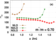
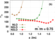
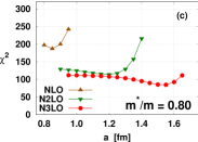
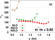
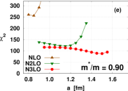
  Figure 1: Penalty functions $\chi^{2}$ obtained in step 2 of the adjustment (see text) as functions of the regulator range $a$. Panels (a)-(e) correspond to the five values of the effective mass adopted in this study.

• Step 3:

  In a consistent effective theory, with increasing order of expansion, the dependence of observables on the range $a$ of the regulator should become weaker and weaker. In our previous work [14], where all terms of the pseudopotential were regulated with the same range, such a behaviour was clearly visible. In the present work, the regulated part of the pseudopotential is combined with two zero-range terms. As a result, even at N³LO, there remains a significant dependence of the penalty functions on $a$, see Fig. 1. Therefore, in step 3 we picked for further analyses the parameterizations of pseudopotentials that correspond to the minimum values of penalty functions.

  Then, for each of the five values of the effective mass and for each of the three orders of expansion, we optimized the corresponding parameters of the pseudopotential, but this time with the infinite-matter properties not rigidly fixed but allowed to change within small tolerance intervals, see Table 1.

In the supplemental material (https://arxiv.org/e-print/2003.10990), the corresponding 15 sets of parameters are listed in a machine readable format. Following the naming convention adopted in Ref. [30], these final sets are named as REG$n$m.190617, where $n$ stands for the order of the pseudopotential ($n=2$ at NLO, $n=4$ at N²LO, and $n=6$ at N³LO), and $\mathrm{m}=\mathrm{a}$, b, c, d, or e stands for one of the five adopted values of the effective mass $m^{*}/m$ 0.70, 0.75, 0.80, 0.85, or 0.90, respectively. For brevity, in the remaining of this paper, we omit the date of the final adjustment, denoted by 190617, which otherwise is an inherent part of the name.

Table 1: Target infinite nuclear matter properties and the corresponding tolerance intervals used in step 3 of the adjustment (see text).

Quantity	$E/A$ [MeV]	$\rho_{\mathrm{sat}}~{}[\mathrm{fm}^{-3}]$	$K_{\infty}$ [MeV]	$m^{*}/m$	$J$ [MeV]	$L$ [MeV]
Value	-16.0	0.158	230	0.70-0.90	29.0	15.00
Tolerance	0.3	0.003	5	0.001	0.5	0.05

We are now in a position to list all contributions to the penalty function $\chi^{2}$, which come from the empirical constrains used in step 3 of the adjustment and from those corresponding to the nuclear data and pseudo-data that we used.

1. Empirical properties of the symmetric infinite nuclear matter. These correspond to: saturation density $\rho_{\mathrm{sat}}$, binding energy per nucleon $E/A$, compression modulus $K_{\infty}$, isoscalar effective mass $m^{*}/m$, symmetry energy coefficient $J$, and its slope $L$. The target values and the corresponding tolerance intervals are listed in Table 1.

2. Potential energies per nucleon in symmetric infinite nuclear matter. We used values in four spin-isospin channels $(S,T)$ determined in theoretical calculations of Refs. [31, 32]. Although it is not clear if these constraints have any significant impact on the observables calculated in finite nuclei, we observed that they seem to prevent the aforementioned numerical instabilities due to compensations of large coupling constants with opposite signs. Explicit formulas for the decomposition of the potential energy in the $(S,T)$ channels are given in A.

3. Energy per nucleon in infinite neutron matter. We used values calculated for potentials UV14 plus UVII (see Table III in [33]) at densities below $0.4~{}\mathrm{fm}^{-3}$ with a tolerance interval of 25 %.

4. Energy per nucleon in polarized infinite nuclear matter. Adjustment of parameters often leads to the appearance of a bound state in symmetric polarized matter. To avoid this type of result, we used the constraint of $E/A=12.52$ MeV at density $0.1\,\mathrm{fm}^{-3}$ (taken from Ref. [34]) with a large tolerance interval of 25 %.

5. Average pairing gap in infinite nuclear matter. Our goal was to obtain a reasonable profile for the average gap in symmetric infinite nuclear matter and to avoid too frequent collapse of pairing for deformed minima (especially for protons). Therefore, we used as targets the values calculated for the D1S functional at $k_{F}=0.4$, $0.8$, and $1.2$ fm^-1 with the tolerance intervals of $0.1$ MeV.

6. Binding energies of spherical nuclei. We used experimental values of the following 17 spherical (or approximated as spherical) nuclei ³⁶Ca, ⁴⁰Ca, ⁴⁸Ca, ⁵⁴Ca, ⁵⁴Ni, ⁵⁶Ni, ⁷²Ni, ⁸⁰Zr, ⁹⁰Zr, ¹¹²Zr, ¹⁰⁰Sn, ¹³²Sn, ¹³⁸Sn, ¹⁷⁸Pb, ²⁰⁸Pb, ²¹⁴Pb, and ²¹⁶Th. We attributed tolerance intervals of 1 MeV (2 MeV) if the binding energy was known experimentally (extrapolated) [35]. The motivation for this list was to use open-shell nuclei along with doubly magic ones, so as to better constrain distances between successive shells.

7. Proton rms radii. We used values taken from Ref. [36] for ⁴⁰Ca, ⁴⁸Ca, ²⁰⁸Pb, and ²¹⁴Pb with the tolerance intervals of 0.02 fm and that for ⁵⁶Ni (which is extrapolated from systematics) with the tolerance interval of 0.03 fm.

8. Isovector and isoscalar central densities. To avoid finite-size scalar-isovector (i.e. $S=0$, $T=1$) instabilities, we used isovector density at the center of ²⁰⁸Pb and isoscalar density at the center of ⁴⁰Ca. A use of the linear response methodology (such as in Ref. [37] for zero-range interactions) would lead to too much time-consuming calculations. As a proxy, we used the two empirical constraints on central densities, which are known to grow uncontrollably when the scalar-isovector instabilities develop. We used the empirical values of $\rho_{1}(0)<0\,\mathrm{fm}^{-3}$ in ²⁰⁸Pb and $\rho_{0}(0)<0.187\,\mathrm{fm}^{-3}$ in ⁴⁰Ca with asymmetric tolerance intervals as described in Ref. [14]. For $\rho_{0}(0)$ in ⁴⁰Ca, we have used the central density obtained with SLy5 [29] as an upper limit. In the parameter adjustments performed in this study, possible instabilities in the vector channels ($S=1$) are still not under control.

9. Surface energy coefficient. As it was recently shown [38, 39], a constraint on the surface energy coefficient is an efficient way to improve properties of EDFs. For the regularized pseudopotentials considered here, we calculate a simple estimate of the surface energy coefficient using a liquid-drop type formula $a_{\mathrm{surf}}^{\mathrm{LDM}}$ with target value of 18.5 MeV and the tolerance interval of 0.2 MeV. The relevance of this constraint and the motivation for the target value are discussed in B.

10. Coupling constants corresponding to vector pairing. Terms of the EDF that correspond to this channel are given in Eq. (36) of Ref. [14]. To avoid transitions to unphysical regions of unrealistically large vector pairing, we constrain them to be equal to $0\pm 5\,\mathrm{MeV}\,\mathrm{fm}^{3}$.

4 Results and discussion

4.1 Parameters and statistical uncertainties

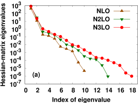
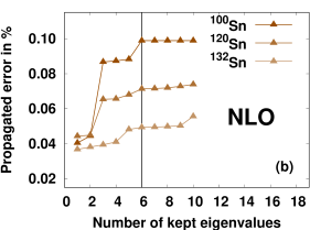
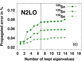
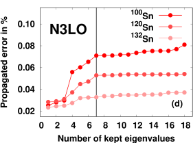
Figure 2: Results of statistical analyses performed for parameterizations corresponding to $m^{*}/m=0.85$. Eigenvalues of the Hessian matrices (a) are compared with propagated uncertainties of binding energies of ¹⁰⁰Sn, ¹²⁰Sn, and ¹³²Sn, determined at NLO REG2d (b), N²LO REG4d (c), and N³LO REG2d (d) plotted as functions of the numbers of eigenvalues kept in the Hessian matrices.

For the purpose of presenting observables calculated in finite nuclei, we decided to use a criterion of binding energies of spherical nuclei, see Sec. 4.3. It then appears that optimal results are obtained for $m^{*}/m=0.85$ at N³LO [40] and $a=1.50$ fm, that is, for the pseudopotential named REG6d. Following this guidance, below we also present some results corresponding to the same effective mass of $m^{*}/m=0.85$ and lower orders: REG2d (NLO and $a=0.85$ fm) and REG4d (N²LO and $a=1.15$ fm). For an extended comparison with the Gogny D1S parameterization [15], which corresponds to $m^{*}/m=0.697$, we also show results for $m^{*}/m=0.70$, that is, for REG6a (N³LO and $a=1.60$ fm). Parameters of the four selected pseudopotentials are tabulated in C. In the supplemental material (https://arxiv.org/e-print/2003.10990) they are collected in a machine readable format.

We performed the standard analysis of statistical uncertainties as presented in Ref. [41]. For REG2d, REG4d and REG6d, eigenvalues of the Hessian matrices corresponding to penalty functions scaled to $\chi^{2}=1$ are shown in Fig, 2(a). The numbers of eigenvalues correspond to the numbers of parameters optimized during the adjustments, and, therefore, vary from 10 (NLO) to 18 (N³LO).

The magnitude of the eigenvalues of the Hessian matrices reveals how well the penalty functions are constrained in the directions of the corresponding eigenvectors in the parameter space. We observe that for the three pseudopotentials considered here, there is a rapid decrease of magnitude from the first to the third eigenvalue and then a slower and almost regular decrease, where no clear gap can be identified. This suggests that all parameters of the pseudopotentials are important.

For three tin isotopes of different nature: ¹⁰⁰Sn (closed-shell, isospin symmetric, unpaired), ¹²⁰Sn (open-shell, isospin asymmetric, paired) and ¹³²Sn (closed-shell, isospin asymmetric, unpaired), we calculated the propagated statistical uncertainties of the total binding energies as functions of the number of kept eigenvalues of the Hessian matrices, Figs 2(b)-(d) for REG2d–REG6d, respectively. For each of the considered parameterizations, after a given number of kept eigenvalues (denoted in Figs 2(b)-(d) by vertical lines), we observe a saturation of the propagated statistical uncertainties. Therefore, we performed the final determination of the statistical uncertainties by keeping these minimal numbers of eigenvalues, i.e. 6 eigenvalues for REG2d (NLO) and 7 for REG4d (N²LO) and REG6d (N³LO).

4.2 Infinite nuclear matter

Table 2: Infinite nuclear matter properties corresponding to pseudopotentials REG2d, REG4d, REG6d, and REG6a, compared to those of the Gogny D1S interaction [15].

Pseudopotential	$E/A$	$\rho_{\mathrm{sat}}$	$K_{\infty}$	$m^{*}/m$	$J$	$L$
	[MeV]	$[\mathrm{fm}^{-3}]$	[MeV]		[MeV]	[MeV]
REG2d	-15.86	0.1574	235.4	0.8499	29.24	14.99
REG4d	-15.86	0.1589	225.6	0.8492	29.17	15.00
REG6d	-15.77	0.1584	232.1	0.8496	28.56	15.00
REG6a	-15.74	0.1564	233.6	0.7014	28.23	15.00
D1S	-16.01	0.1633	202.8	0.6970	31.13	22.44

In Table 2, we list quantities characterizing the properties of infinite nuclear matter. We present results for pseudopotentials REG2d, REG4d, REG6d, and REG6a compared to those characterizing the D1S interaction [15]. For the two strongly constrained quantities, $m^{*}/m$ and $L$, the target values are almost perfectly met, whereas, for the other ones, we observe some deviations, which, nevertheless, are well within the tolerance intervals allowed in the penalty function.

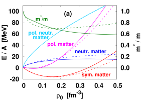
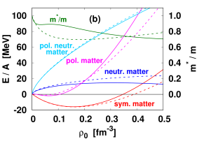
Figure 3: Infinite-nuclear-matter isoscalar effective mass and energies per particle in symmetric, neutron, polarized, and polarized neutron matter as functions of the nuclear density $\rho_{0}$. Results calculated for the D1S interaction [15] (dashed lines) are compared with those obtained for the two pseudopotentials at N³LO with $m^{*}/m=0.70$ (a) and $m^{*}/m=0.85$ (b) (solid lines).

For pseudopotentials REG6a and REG6d, the isoscalar effective mass in symmetric matter and energies per particle (equations of state) for symmetric, neutron, polarized, and polarized neutron matter are plotted in Fig. 3 along with the same quantities for D1S [15]. The plotted equations of state can be obtained from those calculated in four spin-isospin $(S,T)$ channels, see A. For these two N³LO pseudopotentials, equations of state of symmetric matter are somewhat stiffer than that obtained for D1S. This is because of its slightly larger compression modulus $K_{\infty}$. We also can see that for polarized symmetric matter, a shallow bound state appears at low density. This feature also affects D1S. The constraint on the equation of state of polarized symmetric matter introduced in the penalty function has probably limited the development of this state, but did not totally avoid its appearance. Further studies are needed to analyze to what extent it could impact observables calculated in time-odd nuclei and how this possible flaw might be corrected.

The two main differences that appear when we compare the properties in infinite nuclear matter of REG6a and REG6d on one hand and those of D1S on the other hand relate to the equation of state of the neutron matter and isoscalar effective masses. First, near saturation, the regularized pseudopotentials give equations of state of neutron matter slightly lower than D1S, which can be attributed to its lower symmetry energy. Second, for the N³LO pseudopotentials, dependence of the effective on density is less regular than for D1S. We note, however, that the N³LO effective masses are monotonically decreasing functions of the density, and thus the pseudopotentials obtained in this study do not lead to a surface-peaked effective mass, a feature which was expected to improve the description of the density of states around the Fermi energy [42].

4.3 Binding energies, radii, and pairing gaps of spherical nuclei

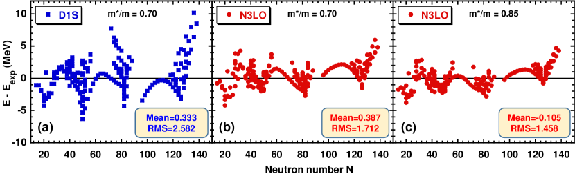
Figure 4: Binding-energy residuals as functions of the neutron number, calculated for a set of spherical nuclei (see text) and plotted for the D1S [15] (a), REG6a (b), and REG6d (c) pseudopotentials.

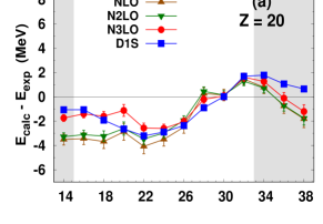
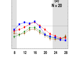
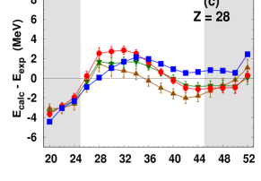
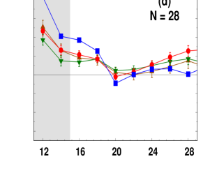
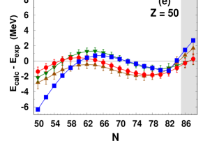
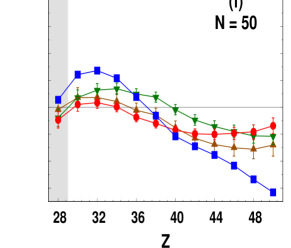
Figure 5: Binding-energy residuals of proton (neutron) semi-magic nuclei with $Z$ ($N$) equal to 20, 28, or 50, plotted in the left (right) panels as functions of the neutron (proton) number, calculated for the REG2d (up triangles), REG4d (down triangles), REG6d (circles), and D1S [15] (squares) pseudopotentials. Shaded zones correspond to the AME2016 masses extrapolated from systematics [35].

In this section, we present results of systematic calculations performed for spherical nuclei and compared with experimental data. For the purpose of such a comparison, we have selected a set of 214 nuclei that were identified as spherical in the systematic calculations performed for the D1S functional in Refs. [43, 44]. In Fig. 4, we present an overview of the binding-energy residuals obtained for the D1S, REG6a, and REG6d functionals. Experimental values were taken from the 2016 atomic mass evaluation [35]. The obtained root-mean-square (RMS) binding-energy residuals are equal to 2.582 MeV for D1S, 1.717 MeV for REG6a, and 1.458 MeV for REG6d. We also see that for REG6d, the trends of binding-energy residuals along isotopic chains in heavy nuclei become much better reproduced. As a reference, we have also determined the analogous RMS value corresponding to the UNEDF0 functional [36, 45], which turns out to be equal to 1.900 MeV.

In Figs. 5 and 6, we show detailed values of binding-energy residuals along the isotopic or isotonic chains of semi-magic nuclei. In most chains one can see a clear improvement of the isospin dependence of masses. In particular, in almost all semi-magic chains, kinks of energy residuals at doubly magic nuclei either decreased or even vanished completely, like at $N=82$ and 126, see Figs. 6(b) and (c), respectively.

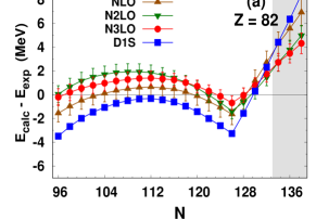
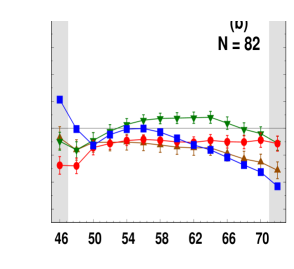
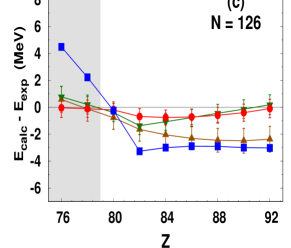
Figure 6: Same as in Fig. 5 but for the semimagic nuclei with $Z=82$, $N=82$ and $N=126$.

In Fig. 7, for the same set of EDFs and nuclei as those used in Fig. 4, we show the analogous residuals of the charge radii of spherical nuclei. The experimental values were taken from Ref. [46]. Again, the N³LO EDFs provide the smallest deviations from data. We note that the residuals of the order of 0.02 fm are typical for many Skyrme-like EDFs, for example, for the UNEDF family of EDFs [6]. Figures 8(a) and (b) present summary of the RMS residuals of binding energies and charge radii, respectively, which were obtained in this study. We see that a decrease of the penalty functions when going from NLO to N²LO, see Fig. 1, is often accompanied by an increase of the RMS residuals. This indicates that the data for 17 spherical nuclei, which are included in the penalty function, see Sec. 3, do not automatically lead to a better description of all spherical nuclei. Only at N³LO a consistently better description is obtained.

Finally, in Figs. 9 and 10, we show calculated average neutron and proton pairing gaps, respectively. Qualitatively, all three EDFs shown in the figures give very similar results. A thorough comparison with experimental odd-even mass staggering, along with parameter adjustments better focused on the pairing channel, will be the subject of a forthcoming publication.

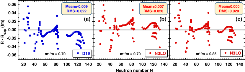
Figure 7: Same as in Fig. 4 but for the charge-radii residuals.

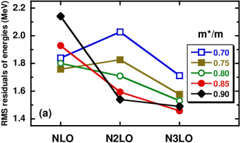
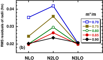
Figure 8: RMS residuals of binding energies (a) and charge radii (b) as functions of the order of pseudopotentials, adjusted in this study for the five values of the isoscalar effective mass $m^{*}/m$.

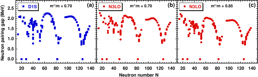
Figure 9: Same as in Fig. 4 but for the average neutron pairing gaps.

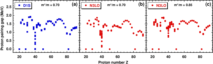
Figure 10: Same as in Fig. 9 but for the average proton pairing gaps.

4.4 Single particle energies

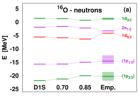
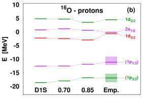
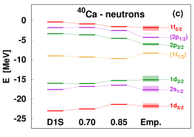
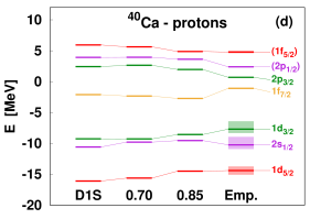
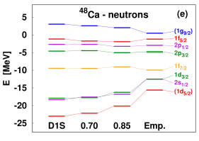
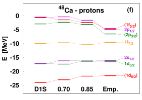
Figure 11: Neutron (left) and proton (right) single-particle energies in ¹⁶O (top), ⁴⁰Ca (middle), and ⁴⁸Ca (bottom), calculated for the D1S [15], REG6a (N³LO, $m^{*}/m=0.70$), and REG6d (N³LO, $m^{*}/m=0.85$) functionals. Empirical values were taken from the compilation of Ref. [47].

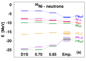
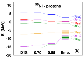
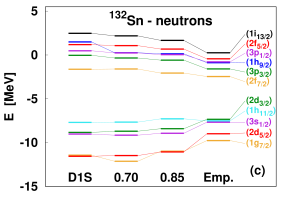
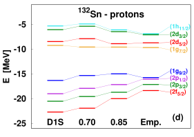
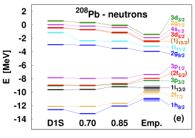
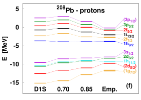
Figure 12: Same as in Fig. 11 but for ⁵⁶Ni (top), ¹³²Sn (middle), and ²⁰⁸Pb (bottom).

In Figs. 11 and 12, we show comparison of single-particle energies calculated in semi-magic nuclei for the D1S [15], REG6a ($m^{*}/m=0.70$), and REG6d ($m^{*}/m=0.85$) functionals with the empirical values taken from the compilation published in the supplemental material of Ref. [47], which contains the single-particle energies collected within three data sets. In all panels of Figs. 11 and 12, horizontal lines of the rightmost columns represent average values of the three data sets, whereas shaded boxes represent spreads between the minimum and maximum values. Quantum numbers in parentheses indicate single-particle states with corresponding attributed spectroscopic factors smaller than 0.8 or unknown.

The spin-orbit interaction corresponding to functional REG6a ($m^{*}/m=0.70$) is smaller than that of D1S, which may explain differences between the single-particle energies of states with large orbital angular momenta. Differences between the results obtained for functionals with $m^{*}/m=0.70$ and $m^{*}/m=0.85$ mostly amount to a global compression. Generally speaking, the calculated single-particle energy spacings are larger than those of the empirical ones, which is typical for the effective masses being smaller than one.

We note that the comparison between the calculated and empirical single-particle energies is given here only for the purpose of illustration. Indeed, both are subjected to uncertainties of definition and meaning. The calculated ones, which are here determined as the eigenenergies of the mean-field Hamiltonian, could also be evaluated from calculated odd-even mass differences. Similarly, determination of the empirical ones is always uncertain from the point of view of the fragmentation of the single-particle strengths. For these reasons, we did not include single-particle energies in the definition of our penalty function, see Sec. 3. Nevertheless, positions and ordering of single-particle energies are crucial for a correct description of other observables, such as, for example, ground-state deformations or deformation energies. Therefore, we consider comparisons presented in Figs. 11 and 12 to be very useful illustrations of properties of the underlying EDFs.

4.5 Deformed nuclei

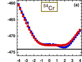
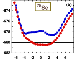
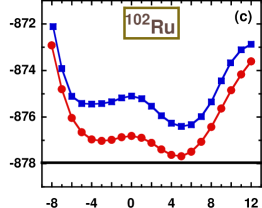
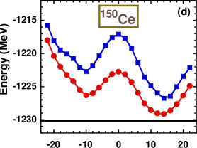
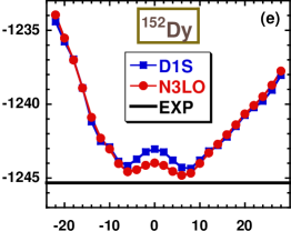
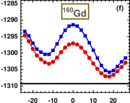
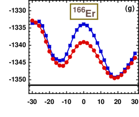
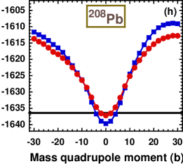
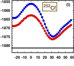
Figure 13: Deformation energies of selected nuclei, calculated for the D1S [15] (squares) and N³LO REG6d (circles) functionals, extrapolated to infinite harmonic-oscillator basis, see D, plotted in the absolute energy scale, and compared with the experimental binding energies [35] (horizontal lines).

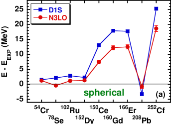
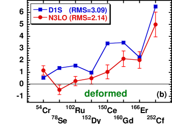
Figure 14: Same as in Fig. 13 but for the binding-energy residuals calculated at spherical shapes (a) and deformed minima (b).

Using the methodology of extrapolating results calculated for $N_{0}=16$ harmonic-oscillator shells to infinite $N_{0}$, presented in D, for a set of nine nuclei from ⁵⁴Cr to ²⁵²Cf we determined deformation energies, Fig. 13, and binding-energy residuals, Fig. 14. The figures compare results obtained for the D1S [15] and N³LO REG6d functionals. For N³LO REG6d, in Fig. 14(a) we also show propagated uncertainties [41] of spherical energies determined using the covariance matrix available in the supplemental material (https://arxiv.org/e-print/2003.10990). For illustration, the same propagated uncertainties are also plotted in Fig. 14(b), whereas determination of full propagated uncertainties of deformed minima is left to a future analysis of deformed solutions.

In general, the pattern of deformations obtained for both functionals is very similar. This is gratifying, because deformed nuclei were not included in the adjustment of either one of the two EDFs. For this admittedly fairly limited sample of nuclei, the pattern of RMS binding-energy residuals is fairly analogous to what we have observed in spherical nuclei, see Sec. 4.3, with REG6d giving values that are about 30% smaller than those for D1S. It is interesting to see that in several instances, the two functionals generate absolute energies of the deformed minima that are more similar to one another than those of the spherical shapes. In the present study we limit ourselves to presenting results only for these very few nuclei, whereas attempts of using deformed nuclei in penalty functions [48] and systematic mass-table calculations [49] are left to forthcoming publications.

5 Conclusions

In this article, we reported on the next step in adjusting parameters of regularized finite-range functional generators to data. We have shown that an order-by-order improvement of agreement with data is possible, and that the sixth order (N³LO) functional describes data similarly or better than the standard Gogny or Skyrme functionals.

We implemented adjustments of parameters based on minimizing fairly complicated penalty function. Our experience shows that a blind optimization to selected experimental data seldom works. Instead, one has to implement sophisticated constraints, which prevent wandering of parameters towards regions where different kinds of instabilities loom.

We consider the process of developing new functionals and adjusting their parameters a continuous effort to better their precision and predictive power. At the expense of introducing single density-dependent generator, here we were able to raise the values of the effective mass, obtained in our previous study [14], well above those that are achievable with purely two-body density-independent generators [19]. Such a solution is perfectly satisfactory at the single-reference level. However, for multi-reference implementations, the density-dependent term must be replaced by second-order three-body zero-range generators [50], or otherwise entirely new yet unknown approach would be required.

Although a definitive conclusion about usefulness of EDFs obtained in this study can only be drawn after a comparison of observables of more diverse nature, this class of pseudopotentials looks promising, even if it can clearly be further improved. In the future, we plan on continuing novel developments by implementing non-local regularized pseudopotentials along with their spin-orbit and tensor terms [13]. This may allow us to fine-tune spectroscopic properties of functionals and facilitate precise description of deformed and odd nuclei.

Appendix A Decomposition of the potential energy in $(S,T)$ channels

The techniques to derive decomposition of the potential energy per particle, $E^{(S,T)}_{\mathrm{pot}}/A$, into four spin-isospin $(S,T)$ channels are the same for finite-range and zero-range pseudopotentials. Therefore, we do not repeat here the details of the derivation, which can be found, for example, in Ref. [51].

First, we recall the expression for the auxiliary function $F_{0}(\xi)$, already introduced in Ref. [30],

$$F_{0}(\xi)=\frac{12}{\xi^{3}}\left[\frac{1-\rme^{-\xi^{2}}}{\xi^{3}}-\frac{3-\rme^{-\xi^{2}}}{2\xi}+\frac{\sqrt{\pi}}{2}\,\mathrm{Erf}\,\xi\right]\,.$$ (5)

Then, in the symmetric infinite nuclear matter with Fermi momentum $k_{F}$ and density $\rho_{0}=2k_{F}^{3}/3\pi^{2}$, contributions of the finite-range local pseudopotential (2) at order zero ($n=0$) to $(S,T)$ channels can be expressed as:

$$\frac{E^{(0,0)}_{\mathrm{pot}}}{A} = \frac{1}{32}\left(W_{1}^{(0)}-B_{1}^{(0)}+H_{1}^{(0)}-M_{1}^{(0)}\right)\rho_{0}\left[1-F_{0}(k_{F}a)\right]\,,$$ (6)

$$\frac{E^{(0,1)}_{\mathrm{pot}}}{A} = \frac{3}{32}\left(W_{1}^{(0)}-B_{1}^{(0)}-H_{1}^{(0)}+M_{1}^{(0)}\right)\rho_{0}\left[1+F_{0}(k_{F}a)\right]\,,$$ (7)

$$\frac{E^{(1,0)}_{\mathrm{pot}}}{A} = \frac{1}{32}\left(W_{1}^{(0)}+B_{1}^{(0)}+H_{1}^{(0)}+M_{1}^{(0)}\right)\rho_{0}\left[1+F_{0}(k_{F}a)\right]\,,$$ (8)

$$\frac{E^{(1,1)}_{\mathrm{pot}}}{A} = \frac{9}{32}\left(W_{1}^{(0)}+B_{1}^{(0)}-H_{1}^{(0)}-M_{1}^{(0)}\right)\rho_{0}\left[1-F_{0}(k_{F}a)\right]\,,$$ (9)

and those at higher orders $n$ as:

$$\frac{E^{(0,0)}_{\mathrm{pot}}}{A} = -\frac{1}{32}\left(W_{1}^{(n)}-B_{1}^{(n)}+H_{1}^{(n)}-M_{1}^{(n)}\right)\rho_{0}\left(-\frac{1}{a}\frac{\partial}{\partial a}\right)^{n/2}F_{0}(k_{F}a)\,,$$ (10)

$$\frac{E^{(0,1)}_{\mathrm{pot}}}{A} = ~{}~{}~{}~{}\frac{3}{32}\left(W_{1}^{(n)}-B_{1}^{(n)}-H_{1}^{(n)}+M_{1}^{(n)}\right)\rho_{0}\left(-\frac{1}{a}\frac{\partial}{\partial a}\right)^{n/2}F_{0}(k_{F}a)\,,$$ (11)

$$\frac{E^{(1,0)}_{\mathrm{pot}}}{A} = ~{}~{}~{}~{}\frac{1}{32}\left(W_{1}^{(n)}+B_{1}^{(n)}+H_{1}^{(n)}+M_{1}^{(n)}\right)\rho_{0}\left(-\frac{1}{a}\frac{\partial}{\partial a}\right)^{n/2}F_{0}(k_{F}a)\,,$$ (12)

$$\frac{E^{(1,1)}_{\mathrm{pot}}}{A} = -\frac{9}{32}\left(W_{1}^{(n)}+B_{1}^{(n)}-H_{1}^{(n)}-M_{1}^{(n)}\right)\rho_{0}\left(-\frac{1}{a}\frac{\partial}{\partial a}\right)^{n/2}F_{0}(k_{F}a)\,.$$ (13)

Appendix B Estimate of the surface energy coefficient

In section 3, we introduced a constraint on the estimate of the surface energy coefficient $a_{\mathrm{surf}}^{\mathrm{LDM}}$, calculated with a liquid-drop-type formula. In the case of local functionals (such as Skyrme functionals), to calculate the surface energy coefficient [38], several approaches can be considered, such as the Hartree-Fock (HF) calculation [52], approximation of the Extended Thomas Fermi (ETF) type [53] or Modified Thomas Fermi (MTF) type [54], or within a leptodermous protocol, which is based on an analysis of calculations performed for very large fictitious nuclei [55].

Some of these approaches are not usable with the regularized pseudopotentials considered in this article. Indeed, the ETF and MTF methods can only be used for functionals that depend on local densities. In principle, the leptodermous protocol could be used, but it would require a significant expense in CPU time. Moreover, the HF calculations cannot be considered because the Friedel oscillations of the density make the extraction of a stable and precise value of the surface energy coefficient very difficult (see discussion in Ref. [38] and references therein).

Therefore, for the purpose of performing parameter adjustments, we decided to use a very simple estimate of the surface energy coefficient, which is usable with any kind of functional. After determining the self-consistent total binding energy $E$ of a fictitious symmetric, spin-saturated, and unpaired $N=Z=40$ nucleus without Coulomb interaction, we used a simple liquid-drop formula to calculate the surface energy coefficient,

$$a_{\mathrm{surf}}^{\mathrm{LDM}}=\frac{E-a_{v}A}{A^{2/3}},$$ (14)

where $A=80$ and $a_{v}$ is the volume energy coefficient in symmetric infinite nuclear matter at the saturation point.

Values of $a_{\mathrm{surf}}^{\mathrm{LDM}}$ obtained in this way do depends on $A$, but, at least in the case Skyrme functionals, they vary linearly with the surface energy coefficients obtained using full HF calculations. Detailed study of the usability of estimates (14) will be the subject of a forthcoming publication [56].

In section 3, we used the value of $a_{\mathrm{surf}}^{\mathrm{LDM}}=18.5$ MeV as the target value of the parameter adjustments. This value is only slightly below the value obtained for the Skyrme functional SLy5s1 (18.6 MeV), which is an improved version of the SLy5 functional with optimized surface properties [38, 39]. This target value we used was only an educated guess, and it may require fine-tuning after a systematic study of the properties of deformed nuclei will have been performed.

Appendix C Parameters of the pseudopotentials

Parameters of the pseudopotentials used in Sec. 4, REG2d at NLO, REG4d at N²LO, and REG6d at N³LO with $m^{*}/m\simeq 0.85$, and REG6a at N³LO with $m^{*}/m\simeq 0.70$ are reported in Table 3 along with their statistical uncertainties. As it turns out, values of parameters rounded to the significant digits, which would be consistent with the statistical uncertainties, give results visibly different than those corresponding to unrounded values. Therefore, in the Table we give all parameters up to the sixth decimal figure. Moreover, the statistical uncertainties of parameters are only given for illustration, whereas the propagated uncertainties of observables have to evaluated using the full covariance matrices [41]. Parameters of other pseudopotentials derived in this study along with the covariance matrix corresponding to REG6d are listed in the supplemental material (https://arxiv.org/e-print/2003.10990).

Table 3: Parameters $a$ (in fm), $t_{3}$ (in MeV fm⁴), $W_{\mathrm{SO}}$ (in MeV fm⁵), and $W_{1}^{(n)}$, $B_{1}^{(n)}$, $H_{1}^{(n)}$, and $M_{1}^{(n)}$ (in MeV fm³⁺ⁿ), of pseudopotentials REG2d, REG4d, REG6d, and REG6a with statistical uncertainties.

	REG2d	REG4d	REG6d	REG6a
	(NLO)	(N2LO)	(N3LO)	(N3LO)
$a$	0.85	1.15	1.50	1.60
$t_{3}$	$11516.477663(0.5)$	$11399.197904(0.1)$	$11509.501921(0.3)$	$9521.936183(0.3)$
$W_{\mathrm{SO}}$	$106.098237(2.8)$	$115.427981(2.2)$	$116.417478(1.9)$	$122.713008(1.9)$
$W_{1}^{(0)}$	$-2510.198547(3.6)$	$-689.651657(2.4)$	$-2253.706132(0.5)$	$-1478.053786(0.9)$
$B_{1}^{(0)}$	$1108.303995(10.0)$	$-824.881825(6.4)$	$740.258749(1.9)$	$87.165128(2.4)$
$H_{1}^{(0)}$	$-2138.673166(2.2)$	$-247.692094(1.1)$	$-1794.716098(2.2)$	$-1031.141021(2.3)$
$M_{1}^{(0)}$	$746.778833(1.6)$	$-1270.827895(2.2)$	$282.583629(1.0)$	$-362.705492(1.3)$
$W_{1}^{(2)}$	$-637.749560(3.7)$	$-741.229448(2.0)$	$-3207.567147(2.1)$	$-2459.995595(2.2)$
$B_{1}^{(2)}$	$210.327285(3.1)$	$434.961848(2.6)$	$2368.246502(1.2)$	$1412.933291(1.6)$
$H_{1}^{(2)}$	$-892.452162(2.3)$	$-951.018473(1.0)$	$-3163.516190(0.8)$	$-2418.882336(0.8)$
$M_{1}^{(2)}$	$379.274480(7.1)$	$615.750351(2.0)$	$2319.605187(0.4)$	$1370.885213(0.6)$
$W_{1}^{(4)}$		$442.206742(3.8)$	$559.364051(1.3)$	$835.586806(2.1)$
$B_{1}^{(4)}$		$-972.382568(2.9)$	$-1398.820389(0.9)$	$-1594.561771(1.2)$
$H_{1}^{(4)}$		$420.867921(4.9)$	$351.670752(1.3)$	$774.195095(1.9)$
$M_{1}^{(4)}$		$-953.687931(2.3)$	$-1197.878374(0.3)$	$-1535.312092(0.5)$
$W_{1}^{(6)}$			$-1603.038264(2.8)$	$-1700.366589(3.8)$
$B_{1}^{(6)}$			$828.626124(2.0)$	$904.903410(2.8)$
$H_{1}^{(6)}$			$-1581.833642(2.0)$	$-1705.515946(2.4)$
$M_{1}^{(6)}$			$802.445641(1.9)$	$914.640430(2.5)$

Appendix D Extrapolation of binding energies of deformed nuclei to infinite harmonic-oscillator basis

In this study, results for spherical nuclei were obtained using code finres₄ [57], which solves HFB equations for finite-range generators on a mesh of points in spherical space coordinates. Because of the spherical symmetry, it is perfectly possible to perform calculations with a mesh dense enough and a number of partial waves high enough for the results to be stable with respect to any change of the numerical conditions. Results for deformed nuclei were obtained using the 3D code hfodd (v2.92a) [58, 59] or axial-symmetry code hfbtemp [60]. These two codes solve HFB equations by expanding single-particle wave functions on harmonic-oscillator bases. Since for deformed nuclei the amount of CPU time and memory is much larger than for spherical ones, it is not practically possible to use enough major harmonic-oscillator shells to reach the asymptotic regime, especially for heavy nuclei.

In order to estimate what would be the converged asymptotic value of the total binding energy of a given deformed nucleus, we proceeded in the following way. First, using code finres₄, we determined the total binding energy $E_{\mathrm{sph}}$ of a given nucleus at the spherical point. Second, using codes hfodd or hfbtemp, for the same nucleus and for a given number of shells $N_{0}$, we determined total binding energies $E_{\mathrm{sph}}(N_{0})$ (constrained to sphericity) and $E_{\mathrm{def}}(N_{0})$ (constrained to a non-zero deformation). Third, we assumed that with $N_{0}\rightarrow\infty$, the deformation energy $\Delta E_{\mathrm{def}}(N_{0})=E_{\mathrm{def}}(N_{0})-E_{\mathrm{sph}}(N_{0})$ converges much faster to its asymptotic value than either of the two energies. Fourth, within this assumption, we estimate the asymptotic energies of deformed nuclei as

$$E_{\mathrm{def}}(N_{0}=\infty)=E_{\mathrm{sph}}+\Delta E_{\mathrm{def}}(N_{0})=E_{\mathrm{def}}(N_{0})+E_{\mathrm{sph}}-E_{\mathrm{sph}}(N_{0}).$$ (15)

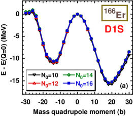
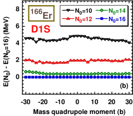
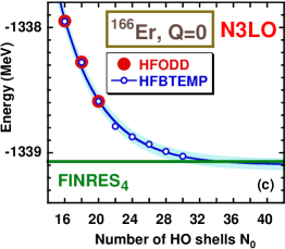
Figure 15: The relative, panels (a) and (b), and absolute, panel (c), binding energies of the spherical point in ¹⁶⁶Er, presented in function of the number $N_{0}$ of harmonic-oscillator shells used in codes hfodd and hfbtemp. In panel (c), the horizontal line represents the asymptotic value determined using code finres₄.

In Fig. 15, we present typical convergence pattern that supports the main assumption leading to estimate (15). Fig. 15(a) shows deformation energies $\Delta E$ of ¹⁶⁶Er calculated for the numbers of shells between $N_{0}=10$ and 16 using the D1S functional [15]. It is clear that in the scale of the figure, differences between the four curves are hardly discernible. In a magnified scale, in Fig. 15(b) we show total energies $E_{\mathrm{def}}(N_{0})-E_{\mathrm{def}}(16)$ relative to that obtained for $N_{0}=16$. We see that at $N_{0}=10$ and 12, the relative energies are fairly flat; however, they also exhibit significant changes, including sudden jumps related to individual orbitals entering and leaving the space of harmonic-oscillator wave functions that are included in the basis with changing deformation. Nevertheless, already at $N_{0}=14$, the relative energy becomes very smooth and almost perfectly flat. This behaviour gives strong support to applying estimate (15) already at $N_{0}=16$. Such a method was indeed used to present all total binding energies of deformed nuclei discussed in this article.

Finally, in Fig. 15(c), in the absolute energy scale we show total binding energies in ¹⁶⁶Er obtained using codes hfodd (up to $N_{0}=20$, large full circles) and hfbtemp (up to $N_{0}=30$, small empty circles). Calculations were constrained to the spherical point and thus the results are directly comparable with the value of $E_{\mathrm{sph}}=-1339.069768$ obtained using the spherical code finres₄ (horizontal line). These results constitute a very strong benchmark of our implementations of the N³LO pseudopotentials in three very different codes. For $N_{0}\leq 20$, differences between the hfodd and hfbtemp total energies (not visible in the scale of the figure) do not exceed 3 keV. By fitting an exponential curve to the hfbtemp results (thin line) we obtained the extrapolated asymptotic value of energy $E_{\mathrm{sph}}(N_{0}=\infty)=-1339.097(34)$, which within the extrapolation error of 34 keV (shown in the figure by the shaded band) perfectly agrees with the finres₄ value.

We thank Ph. Da Costa, M. Bender and J. Meyer for valuable discussions during the development of this project. This work was partially supported by the STFC Grants No. ST/M006433/1 and No. ST/P003885/1, and by the Polish National Science Centre under Contract No. 2018/31/B/ST2/02220. We acknowledge the CSC-IT Center for Science Ltd. (Finland) and the IN2P3 Computing Center (CNRS, Lyon-Villeurbanne, France) for the allocation of computational resources.

References

References

- [1] Bender M, Heenen P H and Reinhard P G 2003 Rev. Mod. Phys. 75(1) 121–180 URL https://link.aps.org/doi/10.1103/RevModPhys.75.121
- [2] Schunck N (ed) 2019 Energy Density Functional Methods for Atomic Nuclei 2053-2563 (IOP Publishing) URL http://dx.doi.org/10.1088/2053-2563/aae0ed
- [3] Robledo L M, Rodríguez T R and Rodríguez-Guzmán R R 2018 Journal of Physics G: Nuclear and Particle Physics 46 013001 URL https://doi.org/10.1088/1361-6471/aadebd
- [4] Bulgac A and Yu Y 2002 Phys. Rev. Lett. 88 042504 (pages 4) URL http://link.aps.org/abstract/PRL/v88/e042504
- [5] Borycki P J, Dobaczewski J, Nazarewicz W and Stoitsov M V 2006 Phys. Rev. C 73(4) 044319 URL https://link.aps.org/doi/10.1103/PhysRevC.73.044319
- [6] Kortelainen M, McDonnell J, Nazarewicz W, Olsen E, Reinhard P G, Sarich J, Schunck N, Wild S M, Davesne D, Erler J and Pastore A 2014 Phys. Rev. C 89(5) 054314 URL http://link.aps.org/doi/10.1103/PhysRevC.89.054314
- [7] Carlsson B G, Dobaczewski J and Kortelainen M 2008 Phys. Rev. C 78(4) 044326 URL http://link.aps.org/doi/10.1103/PhysRevC.78.044326
- [8] Davesne D, Pastore A and Navarro J 2013 Journal of Physics G: Nuclear and Particle Physics 40 095104 URL http://stacks.iop.org/0954-3899/40/i=9/a=095104
- [9] Szpak B, Dobaczewski J, Carlsson B G, Kortelainen M, Michel N, Prassa V, Toivanen J and Veselý P et al., unpublished
- [10] Dobaczewski J, Bennaceur K and Raimondi F 2012 Journal of Physics G: Nuclear and Particle Physics 39 125103 URL http://stacks.iop.org/0954-3899/39/i=12/a=125103
- [11] Castellani E 2002 Stud. Hist. Phil. Mod. Phys. 33 251 (Preprint arXiv:physics/0101039) URL https://arxiv.org/abs/physics/0101039
- [12] Lepage G 1997 nucl-th/9706029 URL https://arxiv.org/abs/nucl-th/9706029
- [13] Raimondi F, Bennaceur K and Dobaczewski J 2014 Journal of Physics G: Nuclear and Particle Physics 41 055112 URL http://stacks.iop.org/0954-3899/41/i=5/a=055112
- [14] Bennaceur K, Idini A, Dobaczewski J, Dobaczewski P, Kortelainen M and Raimondi F 2017 Journal of Physics G: Nuclear and Particle Physics 44 045106 URL http://stacks.iop.org/0954-3899/44/i=4/a=045106
- [15] Berger J, Girod M and Gogny D 1991 Computer Physics Communications 63 365 – 374 URL http://www.sciencedirect.com/science/article/pii/001046559190263K
- [16] Davesne D, Becker Pand Pastore A and Navarro J 2017 Acta Phys. Pol. B 48 265 URL http://www.actaphys.uj.edu.pl/fulltext?series=Reg&vol=48&page=265
- [17] Dobaczewski J, Stoitsov M V, Nazarewicz W and Reinhard P G 2007 Phys. Rev. C 76(5) 054315 URL http://link.aps.org/doi/10.1103/PhysRevC.76.054315
- [18] Sheikh J, Dobaczewski J, Ring P, Robledo L and Yannouleas C 2019 arxiv:1901.06992 URL https://arxiv.org/abs/1901.06992
- [19] Davesne D, Navarro J, Meyer J, Bennaceur K and Pastore A 2018 Phys. Rev. C 97(4) 044304 URL https://link.aps.org/doi/10.1103/PhysRevC.97.044304
- [20] Engel Y, Brink D, Goeke K, Krieger S and Vautherin D 1975 Nuclear Physics A 249 215 – 238 URL http://www.sciencedirect.com/science/article/pii/0375947475901840
- [21] Perlińska E, Rohoziński S G, Dobaczewski J and Nazarewicz W 2004 Phys. Rev. C 69(1) 014316 URL http://link.aps.org/doi/10.1103/PhysRevC.69.014316
- [22] Xu C, Li B A and Chen L W 2010 Phys. Rev. C 82(5) 054607 URL https://link.aps.org/doi/10.1103/PhysRevC.82.054607
- [23] Viñas X, Centelles M, Roca-Maza X and Warda M 2014 The European Physical Journal A 50 27 URL https://doi-org.libproxy.york.ac.uk/10.1140/epja/i2014-14027-8
- [24] Danielewicz P and Lee J 2014 Nuclear Physics A 922 1 – 70 URL http://www.sciencedirect.com/science/article/pii/S0375947413007872
- [25] Dechargé J and Gogny D 1980 Phys. Rev. C 21(4) 1568–1593 URL https://link.aps.org/doi/10.1103/PhysRevC.21.1568
- [26] Goriely S, Hilaire S, Girod M and Péru S 2016 The European Physical Journal A 52 202 URL https://doi-org.libproxy.york.ac.uk/10.1140/epja/i2016-16202-3
- [27] Gonzalez-Boquera C, Centelles M, Viñas X and Robledo L 2018 Physics Letters B 779 195 – 200 URL http://www.sciencedirect.com/science/article/pii/S0370269318301047
- [28] Chabanat E, Bonche P, Haensel P, Meyer J and Schaeffer R 1997 Nuclear Physics A 627 710 – 746 URL http://www.sciencedirect.com/science/article/pii/S0375947497005964
- [29] Chabanat E, Bonche P, Haensel P, Meyer J and Schaeffer R 1998 Nuclear Physics A 635 231 – 256 URL http://www.sciencedirect.com/science/article/pii/S0375947498001808
- [30] Bennaceur K, Dobaczewski J and Raimondi F 2014 EPJ Web of Conferences 66 02031 URL http://dx.doi.org/10.1051/epjconf/20146602031
- [31] Baldo M, Bombaci I and Burgio G F 1997 Astron. Astrophys. 328 274–282 URL http://aa.springer.de/bibs/7328001/2300274/small.htm
- [32] Baldo M 2016 private communication
- [33] Wiringa R B, Fiks V and Fabrocini A 1988 Phys. Rev. C 38(2) 1010–1037 URL https://link.aps.org/doi/10.1103/PhysRevC.38.1010
- [34] Bordbar G H and Bigdeli M 2007 Phys. Rev. C 76(3) 035803 URL https://link.aps.org/doi/10.1103/PhysRevC.76.035803
- [35] Wang M, Audi G, Kondev F, Huang W, Naimi S and Xu X 2017 Chinese Physics C 41 030003 URL http://stacks.iop.org/1674-1137/41/i=3/a=030003
- [36] Kortelainen M, Lesinski T, Moré J, Nazarewicz W, Sarich J, Schunck N, Stoitsov M V and Wild S 2010 Phys. Rev. C 82(2) 024313 URL https://link.aps.org/doi/10.1103/PhysRevC.82.024313
- [37] Hellemans V, Pastore A, Duguet T, Bennaceur K, Davesne D, Meyer J, Bender M and Heenen P H 2013 Phys. Rev. C 88(6) 064323 URL http://link.aps.org/doi/10.1103/PhysRevC.88.064323
- [38] Jodon R, Bender M, Bennaceur K and Meyer J 2016 Phys. Rev. C 94(2) 024335 URL https://link.aps.org/doi/10.1103/PhysRevC.94.024335
- [39] Ryssens W, Bender M, Bennaceur K, Heenen P H and Meyer J 2019 Phys. Rev. C 99(4) 044315 URL https://link.aps.org/doi/10.1103/PhysRevC.99.044315
- [40] Bennaceur K, Dobaczewski J, Haverinen T and Kortelainen M 2019 Regularized pseudopotential for mean-field calculations (Preprint arXiv:1909.12879) URL https://arxiv.org/abs/1909.12879v1
- [41] Dobaczewski J, Nazarewicz W and Reinhard P G 2014 Journal of Physics G: Nuclear and Particle Physics 41 074001 URL http://stacks.iop.org/0954-3899/41/i=7/a=074001
- [42] Ma Z and Wambach J 1983 Nuclear Physics A 402 275 – 300 URL http://www.sciencedirect.com/science/article/pii/0375947483904992
- [43] Delaroche J P, Girod M, Libert J, Goutte H, Hilaire S, Péru S, Pillet N and Bertsch G F 2010 Phys. Rev. C 81(1) 014303 URL https://link.aps.org/doi/10.1103/PhysRevC.81.014303
- [44] Delaroche J P, Girod M, Libert J, Goutte H, Hilaire S, Péru S, Pillet N and Bertsch G F Structure of even-even nuclei using a mapped collective Hamiltonian and the D1S Gogny interaction http://www-phynu.cea.fr/science_en_ligne/carte_potentiels_microscopiques/carte_potentiel_nucleaire_eng.htm
- [45] The massexplorer http://massexplorer.frib.msu.edu/
- [46] Nadjakov E, Marinova K and Gangrsky Y 1994 Atomic Data and Nuclear Data Tables 56 133 – 157 URL http://www.sciencedirect.com/science/article/pii/S0092640X84710047
- [47] Tarpanov D, Dobaczewski J, Toivanen J and Carlsson B G 2014 Phys. Rev. Lett. 113(25) 252501 URL https://link.aps.org/doi/10.1103/PhysRevLett.113.252501
- [48] Haverinen T 2020 et al., to be published
- [49] Kortelainen M 2020 et al., to be published
- [50] Sadoudi J, Duguet T, Meyer J and Bender M 2013 Phys. Rev. C 88(6) 064326 URL http://link.aps.org/doi/10.1103/PhysRevC.88.064326
- [51] Lesinski T, Bennaceur K, Duguet T and Meyer J 2006 Phys. Rev. C 74(4) 044315 URL https://link.aps.org/doi/10.1103/PhysRevC.74.044315
- [52] Côté J and Pearson J 1978 Nuclear Physics A 304 104 – 126 URL http://www.sciencedirect.com/science/article/pii/0375947478900994
- [53] Brack M, Guet C and Håkansson H B 1985 Physics Reports 123 275 – 364 URL http://www.sciencedirect.com/science/article/pii/0370157386900785
- [54] Krivine H and Treiner J 1979 Physics Letters B 88 212 – 215 URL http://www.sciencedirect.com/science/article/pii/0370269379904507
- [55] Reinhard P G, Bender M, Nazarewicz W and Vertse T 2006 Phys. Rev. C 73(1) 014309 URL https://link.aps.org/doi/10.1103/PhysRevC.73.014309
- [56] Da Costa P, Bender M, Bennaceur K, Meyer J and Ryssens W in preparation
- [57] Bennaceur K et al., unpublished
- [58] Schunck N, Dobaczewski J, Satuła W, Ba̧czyk P, Dudek J, Gao Y, Konieczka M, Sato K, Shi Y, Wang X and Werner T 2017 Comp. Phys. Commun. 216 145 – 174 URL http://www.sciencedirect.com/science/article/pii/S0010465517300942
- [59] Dobaczewski J 2020 et al., to be published
- [60] Kortelainen M et al., unpublished