Abstract

In this article, we construct the color-singlet-color-singlet type currents and the color-singlet-color-singlet-color-singlet type currents to study the scalar $D^{*}\bar{D}^{*}$, $D^{*}D^{*}$ tetraquark molecular states and the vector $D^{*}D^{*}\bar{D}^{*}$, $D^{*}D^{*}D^{*}$ hexaquark molecular states with the QCD sum rules in details. In calculations, we choose the pertinent energy scales of the QCD spectral densities with the energy scale formula $\mu=\sqrt{M^{2}_{T}-(2{\mathbb{M}}_{c})^{2}}$ and $\sqrt{M^{2}_{H}-(3{\mathbb{M}}_{c})^{2}}$ for the tetraquark and hexaquark molecular states respectively in a consistent way. We obtain stable QCD sum rules for the scalar $D^{*}\bar{D}^{*}$, $D^{*}D^{*}$ tetraquark molecular states and the vector $D^{*}D^{*}\bar{D}^{*}$ hexaquark molecular state, but cannot obtain stable QCD sum rules for the vector $D^{*}D^{*}D^{*}$ hexaquark molecular state. The connected (nonfactorizable) Feynman diagrams at the tree level (or the lowest order) and their induced diagrams via substituting the quark lines make positive contributions for the scalar $D^{*}D^{*}$ tetraquark molecular state, but make negative or destructive contributions for the vector $D^{*}D^{*}D^{*}$ hexaquark molecular state. It is of no use or meaningless to distinguish the factorizable and nonfactorizable properties of the Feynman diagrams in the color space in the operator product expansion so as to interpret them in terms of the hadronic observables, we can only obtain information about the short-distance and long-distance contributions.

PACS number: 12.39.Mk, 12.38.Lg

Key words: Tetraquark molecular states, Hexaquark molecular states, QCD sum rules

1 Introduction

The QCD sum rules approach, which developed about forty years ago by Shifman, Vainshtein and Zakharov, has become a widely used theoretical tool in studying the hadron properties, such as the masses, decay constants, form-factors, coupling constants, light-cone distribution amplitudes, etc [1, 2, 3]. We carry out the operator product expansion for the correlation functions $\Pi(p^{2})$ in the deep Euclidean space, $P^{2}=-p^{2}\gg\Lambda_{QCD}^{2}$, $t\sim\vec{x}\sim\frac{1}{\sqrt{P^{2}}}$, $x^{2}\sim\frac{1}{P^{2}}$, which represent the short-distance quark-antiquark fluctuations and can be treated in perturbative QCD. A certain energy scale $\mu$ is necessary to separate the regions of the short distance and long distance, the short-distance quark-gluon interactions at the momenta greater than $\mu^{2}$ are included in the Wilson’s coefficients, while the long-distance quark-gluon interactions or soft quark-gluon effects at the momenta less than $\mu^{2}$ are absorbed into the vacuum condensates, which have universal values and are applicable in all the QCD sum rules. On the other hand, at the positive $p^{2}$, the correlation functions $\Pi(p^{2})$ can be expressed in terms of hadronic observables. The correlation functions $\Pi(p^{2})$ obtained at an arbitrary point $p^{2}<0$ relate to the hadron representation through dispersion relation.

Experimentally, a number of charmonium-like and bottomonium-like states, in other words the exotic $X$, $Y$ and $Z$ states, were observed after the observation of the $X(3872)$ by the Belle collaboration [4]. In 2006, R. D. Matheus et al assigned the $X(3872)$ to be the diquark-antidiquark type tetraquark state with the spin-parity-charge-conjugation $J^{PC}=1^{++}$, and studied its mass with the QCD sum rules [5]. Thereafter the QCD sum rules become a powerful theoretical approach in studying the exotic $X$, $Y$, $Z$ and $P_{c}$ states and have given many successful descriptions of the hadron properties, such as the masses and decay widths [6]. As the exotic $X$, $Y$, $Z$ and $P_{c}$ states lie near the meson-meson or meson-baryon thresholds, we can assign them to be the tetraquark or pentaquark molecular states naively and intuitively, and interpolate them with the color-singlet-color-singlet type currents [7, 8, 9, 10].

The color-singlet-color-singlet type currents, which consist of four valance quarks, couple potentially to the tetraquark molecular states, however, the quantum field theory does not forbid the non-vanishing couplings between the color-singlet-color-singlet type currents and meson-meson scattering states. For the color-singlet-color-singlet type currents, Lucha, Melikhov and Sazdjian assert that the Feynman diagrams can be divided into factorizable and nonfactorizable diagrams in the color space, the contributions at the order $\mathcal{O}(\alpha_{s}^{k})$ with $k\leq 1$, which are factorizable in the color space, are exactly canceled out by the meson-meson scattering states at the hadron side, the nonfactorizable diagrams, if having a Landau singularity, begin to make contributions to the tetraquark molecular states, the tetraquark molecular states begin to receive contributions at the order $\mathcal{O}(\alpha_{s}^{2})$ [11, 12]. The assertion is also applicable for the diquark-antidiquark type currents, as they can be rearranged into the color-singlet-color-singlet type currents through the Fierz re-ordering.

In Ref.[13], we provide solid proofs to show that the Landau equation is of no use to study the Feynman diagrams in the QCD sum rules for the tetraquark molecular states and tetraquark states, such as the quarks and gluons are confined objects and thus cannot be put on mass-shell; the operator product expansion is carried out at the region $p^{2}\ll-\Lambda_{QCD}^{2}$ rather than at the region $p^{2}>\Delta^{2}$ to have Landau singularities; the lowest order Feynman diagrams have Landau singularities at the region $p^{2}>\Delta^{2}$, if not assuming the factorizable diagrams in the color space only make contributions to the two-meson scattering states, where the $\Delta^{2}$ denotes the thresholds. We refute the assertion of Lucha, Melikhov and Sazdjian in details, and use two color-singlet-color-singlet type currents as examples to show that the meson-meson scattering states alone cannot saturate the QCD sum rules, while the tetraquark molecular states alone can saturate the QCD sum rules, the tetraquark molecular states begin to receive contributions at the order $\mathcal{O}(\alpha_{s}^{0}/\alpha_{s}^{1})$ rather than at the order $\mathcal{O}(\alpha_{s}^{2})$ [13]. In the light flavor sector, Lee and Kochelev study the two-pion contributions in the QCD sum rules for the scalar meson $f_{0}(600)$ as the tetraquark state, and observe that the contributions at the order $\mathcal{O}(\alpha_{s}^{k})$ with $k\leq 1$ in the operator product expansion cannot be canceled out by the two-pion scattering states [14].

In this article, we extend our previous work to study the $D^{*}\bar{D}^{*}$, $D^{*}D^{*}$, $D^{*}D^{*}\bar{D}^{*}$ and $D^{*}D^{*}D^{*}$ tetraquark and hexaquark molecular states with the QCD sum rules, and examine whether or not it is necessary to distinguish the factorizable and nonfactorizable properties of the Feynman diagrams in the color space so as to interpret them in terms of the hadronic observables. Phenomenologically, the $D^{*}\bar{D}K$, $D^{*}\bar{D}^{*}K$, $D^{*}D^{*}\bar{D}$ and $D^{*}D^{*}\bar{D}^{*}$ hexaquark molecular states have been studied with the heavy quark spin symmetry [15, 16], the $BD\bar{D}$, $BDD$, $DB^{*}\bar{B}^{*}$, $D^{*}B^{*}\bar{B}^{*}$, $DB\bar{B}$ and $D^{*}B\bar{B}$ hexaquark molecular states have been studied with the fixed center approximation to the Faddeev equations [17, 18]. In Ref.[19], we study the $D\bar{D}^{*}K$ hexaquark molecular state with the QCD sum rules by considering the contributions of the vacuum condensates up to dimension-16. In the early works [20, 21, 22], the $D^{*}\bar{D}^{*}$ molecular states were studied via the QCD sum rules by carrying out the operator product expansion up to the vacuum condensates of dimension-6, the Borel platforms were not very flat. In Ref.[23], the $D^{*}\bar{D}^{*}$ molecular states are studied via the QCD sum rules by carrying out the operator product expansion up to the vacuum condensates of dimension-8 and partly taking into account the perturbative corrections to the perturbative terms, however, too large continuum threshold parameters and too large energy scales of the QCD spectral densities are taken. In this article, we study the molecular states of the $D^{*}$-mesons in a consistent way.

The article is arranged as follows: we derive the QCD sum rules for the masses and pole residues of the $D^{*}\bar{D}^{*}$, $D^{*}D^{*}$, $D^{*}D^{*}\bar{D}^{*}$ and $D^{*}D^{*}D^{*}$ tetraquark and hexaquark molecular states, and examine the properties of the Feynman diagrams in Sect.2; in Sect.3, we present the numerical results and discussions; and Sect.4 is reserved for our conclusion.

2 QCD sum rules for the tetraquark and hexaquark molecular states

Firstly, let us write down the two-point correlation functions $\Pi(p)$ and $\Pi_{\mu\nu}(p)$ in the QCD sum rules,

$$\Pi(p) = i\int d^{4}xe^{ip\cdot x}\langle 0|T\Big{\{}J(x)J^{\dagger}(0)\Big{\}}|0\rangle\,,$$

$$\Pi_{\mu\nu}(p) = i\int d^{4}xe^{ip\cdot x}\langle 0|T\Big{\{}J_{\mu}(x)J^{\dagger}_{\nu}(0)\Big{\}}|0\rangle\,,$$ (1)

where $J(x)=J_{c\bar{c}}(x)$, $J_{cc}(x)$, $J_{\mu}(x)=J^{cc\bar{c}}_{\mu}(x)$, $J^{ccc}_{\mu}(x)$,

$$J_{c\bar{c}}(x) = \bar{c}(x)\gamma_{\alpha}q(x)\,\bar{q}(x)\gamma^{\alpha}c(x)\,,$$

$$J_{cc}(x) = \bar{q}(x)\gamma_{\alpha}c(x)\,\bar{q}(x)\gamma^{\alpha}c(x)\,,$$

$$J^{cc\bar{c}}_{\mu}(x) = \bar{c}(x)\gamma_{\alpha}q(x)\,\bar{q}(x)\gamma^{\alpha}c(x)\,\bar{q}(x)\gamma_{\mu}c(x)\,,$$

$$J^{ccc}_{\mu}(x) = \bar{q}(x)\gamma_{\alpha}c(x)\,\bar{q}(x)\gamma^{\alpha}c(x)\,\bar{q}(x)\gamma_{\mu}c(x)\,,$$ (2)

where $q=u$ or $d$. The color-singlet-color-singlet type currents $J_{c\bar{c}}(x)$ and $J_{cc}(x)$ couple potentially to the scalar hidden-charm and doubly charmed tetraquark molecular states or two-meson scattering states, respectively, the color-singlet-color-singlet-color-singlet type currents $J^{cc\bar{c}}_{\mu}(x)$ and $J^{ccc}_{\mu}(x)$ couple potentially to the vector charmed plus hidden-charm and triply charmed hexaquark molecular states or three-meson scattering states, respectively. The currents $J_{c\bar{c}}(x)$, $J_{cc}(x)$, $J^{cc\bar{c}}_{\mu}(x)$ and $J^{ccc}_{\mu}(x)$ have the isospins $I=0$, $1$, $\frac{1}{2}$ and $\frac{3}{2}$, respectively. In the isospin limit, the currents with the same isospins couple potentially to the hadrons or hadron-systems with almost degenerated masses.

At the hadron side of the correlation functions $\Pi(p)$ and $\Pi_{\mu\nu}(p)$, we isolate the contributions of the lowest hidden-charm and doubly-charmed tetraquark molecular states and the charmed plus hidden-charm and triply-charmed hexaquark molecular states to obtain the hadron representation,

$$\Pi(p) = \frac{\lambda_{T}^{2}}{M_{T}^{2}-p^{2}}+\cdots=\Pi_{T}(p^{2})\,,$$

$$\Pi_{\mu\nu}(p) = \frac{\lambda_{H}^{2}}{M_{H}^{2}-p^{2}}\left(-g_{\mu\nu}+\frac{p_{\mu}p_{\nu}}{p^{2}}\right)+\cdots\,,$$ (3)

$$= \Pi_{H}(p^{2})\left(-g_{\mu\nu}+\frac{p_{\mu}p_{\nu}}{p^{2}}\right)+\cdots\,,$$

where the subscripts $T$ and $H$ denote the scalar $D^{*}\bar{D}^{*}$, $D^{*}D^{*}$ tetraquark molecular states and the vector $D^{*}D^{*}\bar{D}^{*}$, $D^{*}D^{*}D^{*}$ hexaquark molecular states, respectively, and we have used the definitions for the pole residues,

$$\langle 0|J(0)|T(p)\rangle = \lambda_{T}\,,$$

$$\langle 0|J_{\mu}(0)|H(p)\rangle = \lambda_{H}\,\varepsilon_{\mu}\,,$$ (4)

the $\varepsilon_{\mu}$ are the polarization vectors of the vector hexaquark molecular states. In Ref.[13], we observe that, for the color-singlet-color-singlet type currents, the meson-meson scattering states alone cannot saturate the QCD sum rules, while the tetraquark molecular states alone can saturate the QCD sum rules, the net effects of the two-meson scattering states amount to modifying the pole residues considerably without influencing the predicted masses. In this article, we only take into account the tetraquark and hexaquark molecular states, as the widths of those molecular states, which absorb the contributions of the two-meson or three-meson scattering states, are unknown.

At the QCD side of the correlation functions $\Pi(p)$ and $\Pi_{\mu\nu}(p)$, we contract the $q$ and $c$ quark fields with the Wick’s theorem, and obtain the results,

$$\Pi_{c\bar{c}}(p) = i\int d^{4}x\,e^{ip\cdot x}\,{\rm Tr}\left[\gamma_{\alpha}S^{ij}(x)\gamma_{\beta}C^{ji}(-x)\right]{\rm Tr}\left[\gamma^{\alpha}C^{nm}(x)\gamma^{\beta}S^{mn}(-x)\right]\,,$$ (5)

$$\Pi_{cc}(p) = 2i\int d^{4}x\,e^{ip\cdot x}\,\Big{\{}{\rm Tr}\left[\gamma_{\alpha}C^{ij}(x)\gamma_{\beta}S^{ji}(-x)\right]{\rm Tr}\left[\gamma^{\alpha}C^{nm}(x)\gamma^{\beta}S^{mn}(-x)\right]$$ (6)

$$-{\rm Tr}\left[\gamma_{\alpha}C^{ij}(x)\gamma_{\beta}S^{jk}(-x)\gamma^{\alpha}C^{km}(x)\gamma^{\beta}S^{mi}(-x)\right]\Big{\}}\,,$$

$$\Pi^{cc\bar{c}}_{\mu\nu}(p) = i\int d^{4}x\,e^{ip\cdot x}$$ (7)

$$\Big{\{}-{\rm Tr}\left[\gamma_{\alpha}S^{ij}(x)\gamma_{\beta}C^{ji}(-x)\right]{\rm Tr}\left[\gamma^{\alpha}C^{km}(x)\gamma^{\beta}S^{mk}(-x)\right]{\rm Tr}\left[\gamma_{\mu}C^{ln}(x)\gamma_{\nu}S^{nl}(-x)\right]$$

$$-{\rm Tr}\left[\gamma_{\alpha}S^{ij}(x)\gamma_{\beta}C^{ji}(-x)\right]{\rm Tr}\left[\gamma^{\alpha}C^{km}(x)\gamma_{\nu}S^{mk}(-x)\right]{\rm Tr}\left[\gamma_{\mu}C^{ln}(x)\gamma^{\beta}S^{nl}(-x)\right]$$

$$+{\rm Tr}\left[\gamma_{\alpha}S^{ij}(x)\gamma_{\beta}C^{ji}(-x)\right]{\rm Tr}\left[\gamma^{\alpha}C^{km}(x)\gamma^{\beta}S^{ml}(-x)\gamma_{\mu}C^{ln}(x)\gamma_{\nu}S^{nk}(-x)\right]$$

$$+{\rm Tr}\left[\gamma_{\alpha}S^{ij}(x)\gamma_{\beta}C^{ji}(-x)\right]{\rm Tr}\left[\gamma^{\alpha}C^{km}(x)\gamma_{\nu}S^{ml}(-x)\gamma_{\mu}C^{ln}(x)\gamma^{\beta}S^{nk}(-x)\right]\Big{\}}\,,$$

$$\Pi^{ccc}_{\mu\nu}(p) = 2i\int d^{4}x\,e^{ip\cdot x}$$ (8)

$$\Big{\{}-{\rm Tr}\left[\gamma_{\alpha}C^{ij}(x)\gamma_{\beta}S^{ji}(-x)\right]{\rm Tr}\left[\gamma^{\alpha}C^{kl}(x)\gamma^{\beta}S^{lk}(-x)\right]{\rm Tr}\left[\gamma_{\mu}C^{mn}(x)\gamma_{\nu}S^{nm}(-x)\right]$$

$$-2{\rm Tr}\left[\gamma_{\alpha}C^{ij}(x)\gamma_{\beta}S^{ji}(-x)\right]{\rm Tr}\left[\gamma^{\alpha}C^{kl}(x)\gamma_{\nu}S^{lk}(-x)\right]{\rm Tr}\left[\gamma_{\mu}C^{mn}(x)\gamma^{\beta}S^{nm}(-x)\right]$$

$$+2{\rm Tr}\left[\gamma_{\alpha}C^{ij}(x)\gamma_{\beta}S^{ji}(-x)\right]{\rm Tr}\left[\gamma^{\alpha}C^{kl}(x)\gamma^{\beta}S^{lm}(-x)\gamma_{\mu}C^{mn}(x)\gamma_{\nu}S^{nk}(-x)\right]$$

$$+2{\rm Tr}\left[\gamma_{\alpha}C^{ij}(x)\gamma_{\beta}S^{ji}(-x)\right]{\rm Tr}\left[\gamma^{\alpha}C^{kl}(x)\gamma_{\nu}S^{lm}(-x)\gamma_{\mu}C^{mn}(x)\gamma^{\beta}S^{nk}(-x)\right]$$

$$+2{\rm Tr}\left[\gamma_{\alpha}C^{ij}(x)\gamma_{\nu}S^{ji}(-x)\right]{\rm Tr}\left[\gamma^{\alpha}C^{kl}(x)\gamma_{\beta}S^{lm}(-x)\gamma_{\mu}C^{mn}(x)\gamma^{\beta}S^{nk}(-x)\right]$$

$$+2{\rm Tr}\left[\gamma_{\mu}C^{ij}(x)\gamma_{\beta}S^{ji}(-x)\right]{\rm Tr}\left[\gamma_{\alpha}C^{kl}(x)\gamma^{\beta}S^{lm}(-x)\gamma^{\alpha}C^{mn}(x)\gamma_{\nu}S^{nk}(-x)\right]$$

$$+{\rm Tr}\left[\gamma_{\mu}C^{ij}(x)\gamma_{\nu}S^{ji}(-x)\right]{\rm Tr}\left[\gamma_{\alpha}C^{kl}(x)\gamma_{\beta}S^{lm}(-x)\gamma^{\alpha}C^{mn}(x)\gamma^{\beta}S^{nk}(-x)\right]$$

$$-2{\rm Tr}\left[\gamma_{\alpha}C^{ij}(x)\gamma_{\beta}S^{jk}(-x)\gamma^{\alpha}C^{kl}(x)\gamma^{\beta}S^{lm}(-x)\gamma_{\mu}C^{mn}(x)\gamma_{\nu}S^{ni}(-x)\right]$$

$$-2{\rm Tr}\left[\gamma_{\alpha}C^{ij}(x)\gamma_{\beta}S^{jk}(-x)\gamma^{\alpha}C^{kl}(x)\gamma_{\nu}S^{lm}(-x)\gamma_{\mu}C^{mn}(x)\gamma^{\beta}S^{ni}(-x)\right]$$

$$-2{\rm Tr}\left[\gamma_{\alpha}C^{ij}(x)\gamma_{\nu}S^{jk}(-x)\gamma^{\alpha}C^{kl}(x)\gamma_{\beta}S^{lm}(-x)\gamma_{\mu}C^{mn}(x)\gamma^{\beta}S^{ni}(-x)\right]\Big{\}}\,,$$

where the $S_{ij}(x)$ and $C_{ij}(x)$ are the full light and heavy quark propagators, respectively,

$$S_{ij}(x) = \frac{i\delta_{ij}\!\not\!{x}}{2\pi^{2}x^{4}}-\frac{\delta_{ij}\langle\bar{q}q\rangle}{12}-\frac{\delta_{ij}x^{2}\langle\bar{q}g_{s}\sigma Gq\rangle}{192}-\frac{ig_{s}G^{a}_{\alpha\beta}t^{a}_{ij}(\!\not\!{x}\sigma^{\alpha\beta}+\sigma^{\alpha\beta}\!\not\!{x})}{32\pi^{2}x^{2}}$$ (9)

$$-\frac{\delta_{ij}x^{4}\langle\bar{q}q\rangle\langle g_{s}^{2}GG\rangle}{27648}-\frac{1}{8}\langle\bar{q}_{j}\sigma^{\mu\nu}q_{i}\rangle\sigma_{\mu\nu}+\cdots\,,$$

$$C_{ij}(x) = \frac{i}{(2\pi)^{4}}\int d^{4}ke^{-ik\cdot x}\left\{\frac{\delta_{ij}}{\!\not\!{k}-m_{c}}-\frac{g_{s}G^{n}_{\alpha\beta}t^{n}_{ij}}{4}\frac{\sigma^{\alpha\beta}(\!\not\!{k}+m_{c})+(\!\not\!{k}+m_{c})\sigma^{\alpha\beta}}{(k^{2}-m_{c}^{2})^{2}}\right.$$

$$\left.-\frac{g_{s}^{2}(t^{a}t^{b})_{ij}G^{a}_{\alpha\beta}G^{b}_{\mu\nu}(f^{\alpha\beta\mu\nu}+f^{\alpha\mu\beta\nu}+f^{\alpha\mu\nu\beta})}{4(k^{2}-m_{c}^{2})^{5}}+\cdots\right\}\,,$$

$$f^{\alpha\beta\mu\nu} = (\!\not\!{k}+m_{c})\gamma^{\alpha}(\!\not\!{k}+m_{c})\gamma^{\beta}(\!\not\!{k}+m_{c})\gamma^{\mu}(\!\not\!{k}+m_{c})\gamma^{\nu}(\!\not\!{k}+m_{c})\,,$$ (10)

and $t^{n}=\frac{\lambda^{n}}{2}$, the $\lambda^{n}$ is the Gell-Mann matrix [2, 24, 25], we add the subscripts $c\bar{c}$, $cc$, $cc\bar{c}$ and $ccc$ to denote the corresponding currents. In the full light quark propagator, see Eq.(9), we add the term $\langle\bar{q}_{j}\sigma_{\mu\nu}q_{i}\rangle$, which comes from the Fierz rearrangement of the quark-antiquark pair $\langle q_{i}\bar{q}_{j}\rangle$ to absorb the gluons emitted from other quark lines to extract the mixed condensates $\langle\bar{q}g_{s}\sigma Gq\rangle$, $\langle\bar{q}g_{s}\sigma Gq\rangle^{2}$ and $\langle\bar{q}g_{s}\sigma Gq\rangle^{3}$, respectively [24].

In Eqs.(5)-(8), we assume dominance of the vacuum intermediate state tacitly, and insert the vacuum intermediate state in all the channels and neglect the contributions of all the other states. In the original works, Shifman, Vainshtein and Zakharov took the factorization hypothesis according to two reasons [1]. One is the rather large value of the quark condensate $\langle\bar{q}q\rangle$, the other is the duality between the quark and physical states, which implies that counting both the quark and physical states may well become a double counting since they reproduce each other [1].

In the QCD sum rules for the traditional mesons, we usually introduce a parameter $\kappa$ to parameterize the deviation from the factorization hypothesis by hand [26], for example, in the case of the four quark condensate, $\langle\bar{q}q\rangle^{2}\to\kappa\langle\bar{q}q\rangle^{2}$ [26, 27]. In fact, the vacuum saturation works well in the large $N_{c}$ limit [28]. As the $\langle\bar{q}q\rangle^{2}$ is always companied with the fine-structure constant $\alpha_{s}=\frac{g_{s}^{2}}{4\pi}$, and plays a minor important role, the deviation from $\kappa=1$, for example, $\kappa=2\sim 3$, cannot make much difference, though the value $\kappa>1$ can lead to better QCD sum rules in some cases.

However, in the QCD sum rules for the tetraquark, pentaquark and hexaquark (molecular) states, the four-quark condensate plays an important role, a large value, for example, $\kappa=2$, can destroy the platforms in the QCD sum rules for the current $J_{c\bar{c}}(x)$. In calculations, we observe that the optimal value is $\kappa=1$, the vacuum saturation works well in the QCD sum rules for the multiquark states.

Up to now, all the multiquark states are studied with the procedure illustrated in Eqs.(5)-(2) by assuming the vacuum saturation for the higher dimensional vacuum condensates tacitly in performing the operator product expansion, except for in some case the parameter $\kappa$ is introduced for the sake of fine-tuning [23]. The true values of the higher dimensional vacuum condensates, even the four quark condensates $\langle\bar{q}\Gamma q\bar{q}\Gamma^{\prime}q\rangle$, remain unknown or poorly known, where the $\Gamma$ and $\Gamma^{\prime}$ stand for the Dirac $\gamma$-matrixes, we cannot obtain robust estimations about the effects beyond the vacuum saturation.

In the QCD sum rules for the multiquark states, such as the tetraquark, pentaquark and hexaquark (molecular) states, we often encounter the vacuum condensates $\langle\bar{q}q\rangle^{2}$ and $\langle\bar{q}q\rangle^{3}$, we have the choice to introduce the parameter $\kappa$ to parameterize the deviation from the factorization hypothesis, although the most commonly used value $\kappa=1$ works well. If the true value $\kappa>1$ or $\gg 1$, the QCD sum rules for the tetraquark, pentaquark and hexaquark (molecular) states have considerably larger systematic uncertainties and are less reliable than those of traditional mesons and baryons [29]. In this respect, we make predictions for the multiquark masses with the QCD sum rules based on the vacuum saturation (i.e. $\kappa=1$), then confront them to the experimental data in the future to test the theoretical calculations. We can also choose the value $\kappa>1$ and obtain predictions to be compared with the experimental data in the future. Many works are still needed to obtain the pertinent value of the $\kappa$.

We usually neglect the tadpole-like contributions from the contractions of the light quarks in the same currents in the QCD sum rules for the multiquark states. For the currents $J_{c\bar{c}}(x)$ and $J^{cc\bar{c}}_{\mu}(x)$, if we contract the light quarks in the same currents, we can obtain the following tadpole-like contributions,

$$J_{c\bar{c}}(x) \to \hat{J}_{c\bar{c}}(x)=-\frac{\langle\bar{q}q\rangle}{3}\bar{c}(x)c(x)\,,$$

$$J^{cc\bar{c}}_{\mu}(x) \to \hat{J}^{cc\bar{c}}_{\mu}(x)=-\frac{5\langle\bar{q}q\rangle}{12}\bar{c}(x)c(x)\,\bar{q}(x)\gamma_{\mu}c(x)-\frac{i\langle\bar{q}q\rangle}{12}\bar{c}(x)\sigma_{\mu\alpha}c(x)\,\bar{q}(x)\gamma^{\alpha}c(x)\,.$$ (11)

The induced currents $\hat{J}_{c\bar{c}}(x)$ and $\hat{J}^{cc\bar{c}}_{\mu}(x)$ have two and four valence quarks, respectively, and they are irrelevant in the present case and can be neglected safely.

Now let us compute the integrals both in the coordinate space and momentum space in Eqs.(5)-(8) to obtain the correlation functions $\Pi_{T}(p^{2})$ and $\Pi_{H}(p^{2})$ at the quark-gluon level, and then obtain the QCD spectral densities through dispersion relation,

$$\rho_{T/H,QCD}(s) = {\rm lim}_{\epsilon\to 0}\frac{{\rm Im}\Pi_{T/H}(s+i\epsilon)}{\pi}\,,$$ (12)

the QCD spectral densities $\rho_{T,QCD}(s)$ are given explicitly in the appendix, while the analytical expressions of the QCD spectral densities $\rho_{H,QCD}(s)$ are too cumbersome, the interested readers can contract me via E-mail to obtain them.

All the contributions in the operator product expansion can be shown explicitly using the Feynman diagrams. In the Feynman diagrams drawn in Figs.1-5, we show the lowest order contributions. If we substitute the light and heavy quark lines with the full light and heavy quark propagators in Eqs.(9)-(2), respectively, we can obtain all the Feynman diagrams. From the figures, we can see that there are only factorizable contributions in the color space for the currents $J_{c\bar{c}}(x)$ and $J_{\mu}^{cc\bar{c}}(x)$, while there are both factorizable and nonfactorizable contributions in the color space for the currents $J_{cc}(x)$ and $J_{\mu}^{ccc}(x)$. There are also nonfactorizable sub-clusters in the Feynman diagrams for the current $J_{\mu}^{cc\bar{c}}(x)$, see the second and the third diagrams in Fig.3. Thereafter, we will use the nomenclatures ”factorizable contributions” and ”nonfactorizable contributions” to denote the contributions come from the factorizable and nonfactorizable Feynman diagrams in the color space, respectively.

From the factorizable diagrams, see Fig.1 and Figs.3-4, we can obtain both the factorizable and nonfactorizable diagrams, while from the nonfactorizable diagrams, see Fig.2 and Fig.5, we can obtain only the nonfactorizable diagrams. Lucha, Melikhov and Sazdjian assert that those nonfactorizable Feynman diagrams shown in Fig.2 and Fig.5 can be deformed into the box diagrams [12]. It is unfeasible, those nonfactorizable Feynman diagrams can only be deformed into the box diagrams in the color space, not in the momentum space.

Figure 1: The Feynman diagram for the lowest order contribution for the current $J_{c\bar{c}}(x)$, where the solid lines and dashed lines represent the light quarks and heavy quarks, respectively.

Figure 2: The Feynman diagrams for the lowest order contributions for the current $J_{cc}(x)$, where the solid lines and dashed lines represent the light quarks and heavy quarks, respectively.

Figure 3: The Feynman diagrams for the lowest order contributions for the current $J_{\mu}^{cc\bar{c}}(x)$, where the solid lines and dashed lines represent the light quarks and heavy quarks, respectively.

Figure 4: The factorizable Feynman diagrams in the color space for the lowest order contributions for the current $J_{\mu}^{ccc}(x)$, where the solid lines and dashed lines represent the light quarks and heavy quarks, respectively.

Figure 5: The nonfactorizable Feynman diagrams in the color space for the lowest order contributions for the current $J_{ccc}(x)$, where the solid lines and dashed lines represent the light quarks and heavy quarks, respectively, the other diagrams obtained by interchanging of the three vertexes at the point $0$ or $x$ are implied.

Figure 6: The typical Feynman diagrams which can be factorized into two colored quark lines for the conventional heavy mesons, where the solid line and dashed line denote the light quark and heavy quark, respectively.

Figure 7: The typical Feynman diagrams which cannot be factorized into two colored quark lines for the conventional heavy mesons, where the solid line and dashed line denote the light quark and heavy quark, respectively.

According to the assertion of Lucha, Melikhov and Sazdjian [11, 12], the factorizable (disconnected) diagrams in the color space only make contributions to the meson-meson scattering states. From the lowest Feynman diagrams shown in Figs.1-5, we can draw the conclusion tentatively that we can obtain more good QCD sum rules from the currents $J_{cc}(x)$ and $J^{ccc}_{\mu}(x)$ than from the currents $J_{c\bar{c}}(x)$ and $J^{cc\bar{c}}_{\mu}(x)$, as there are connected (nonfactorizable) diagrams besides disconnected (factorizable) diagrams.

In fact, it is useless to distinguish the factorizable and nonfactorizable properties of the Feynman diagrams in the operator product expansion, where the short-distance contributions above a certain energy scale $\mu$ are included in the Wilson’s coefficients, the long-distance contributions below the special energy scale $\mu$ are included in the vacuum condensates. In general, we can choose any energy scales at which the perturbative QCD calculations are feasible. Besides the uncertainties originate from the energy scales, additional uncertainties come from the fact that it is impossible to separate the soft tails in the quark-loop diagrams using the standard Feynman-diagram technique. We cannot obtain the information asserted by Lucha, Melikhov and Sazdjian from the Feynman diagrams in the operator product expansion [11, 12], we can only obtain information about the short-distance and long-distance contributions.

We can borrow some ideas from the QCD sum rules for the conventional heavy mesons, in which the hadronic spectral densities can be written as,

$$\rho_{H}(s) = f_{H}^{2}m_{H}^{2}\delta(s-m_{H}^{2})+\rho_{QCD}(s)\Theta(s-s_{0})\,,$$ (13)

where the subscript $H$ denotes the $D$ and $B$ mesons, the $f_{H}$ are the decay constants, the hadronic spectral densities above the continuum thresholds $s_{0}$ are approximated by the perturbative contributions as only the perturbative contributions are left. In the operator product expansion, we often encounter the Feynman diagrams shown in Figs.6-7, the Feynman diagrams shown in Fig.6 (Fig.7) can be (cannot be) factorized into two colored quark lines. Analogously, could we assert that the Feynman diagrams shown in Fig.6 can be exactly canceled out by two asymptotic quarks, only the Feynman diagrams shown in Fig.7 make contributions to the heavy mesons? In Ref.[30], Lucha, Melikhov and Simula take into account all those Feynman diagrams, which is in contrast to the assertion of Lucha, Melikhov and Sazdjian in Refs.[11, 12].

In the QCD sum rules for the tetraquark (molecular) states, pentaquark (molecular) states and hexaquark states (or dibaryon states), we take into account the vacuum condensates, which are vacuum expectations of the quark-gluon operators of the order $\mathcal{O}(\alpha_{s}^{k})$ with $k\leq 1$ in a consistent way [8, 13, 24, 31, 32, 33, 34, 35].

There are two light quark lines and two heavy quark lines in the Feynman diagrams in Figs.1-2, while there are three light quark lines and three heavy quark lines in Figs.3-5, if each heavy quark line emits a gluon and each light quark line contributes quark-antiquark pair, we obtain the quark-gluon operators $g_{s}G_{\mu\nu}g_{s}G_{\alpha\beta}\bar{q}q\bar{q}q$ and $g_{s}G_{\mu\nu}g_{s}G_{\alpha\beta}g_{s}G_{\lambda\tau}\bar{q}q\bar{q}q\bar{q}q$ from the Figs.1-2 and Figs.3-5, respectively, which are of dimension 10 and 15, respectively. The operator $g_{s}G_{\mu\nu}g_{s}G_{\alpha\beta}\bar{q}q\bar{q}q$ leads to the vacuum condensates $\langle\frac{\alpha_{s}GG}{\pi}\rangle\langle\bar{q}q\rangle^{2}$ and $\langle\bar{q}g_{s}\sigma Gq\rangle^{2}$, while the operator $g_{s}G_{\mu\nu}g_{s}G_{\alpha\beta}g_{s}G_{\lambda\tau}\bar{q}q\bar{q}q\bar{q}q$ leads to the vacuum condensates $\langle\frac{\alpha_{s}GG}{\pi}\rangle\langle\bar{q}q\rangle^{2}\langle\bar{q}g_{s}\sigma Gq\rangle$, $\langle g_{s}^{3}GGG\rangle\langle\bar{q}q\rangle^{3}$ and $\langle\bar{q}g_{s}\sigma Gq\rangle^{3}$.

In the present case, if taking the truncation $k\leq 1$ for the quark-gluon operators, for the correlation function $\Pi(p)$, the highest dimensional vacuum condensates are $\langle\bar{q}q\rangle^{2}\langle\frac{\alpha_{s}GG}{\pi}\rangle$ and $\langle\bar{q}g_{s}\sigma Gq\rangle^{2}$, which are of dimension 10, while for the correlation function $\Pi_{\mu\nu}(p)$, the highest dimensional vacuum condensates are $\langle\bar{q}q\rangle^{3}\langle\frac{\alpha_{s}GG}{\pi}\rangle$ and $\langle\bar{q}q\rangle\langle\bar{q}g_{s}\sigma Gq\rangle^{2}$, which are of dimension 13. The vacuum condensates $\langle\frac{\alpha_{s}GG}{\pi}\rangle\langle\bar{q}q\rangle^{2}\langle\bar{q}g_{s}\sigma Gq\rangle$, $\langle g_{s}^{3}GGG\rangle\langle\bar{q}q\rangle^{3}$ and $\langle\bar{q}g_{s}\sigma Gq\rangle^{3}$, which are of dimension 15, come from the quark-gluon operators of the order $\mathcal{O}(\alpha_{s}^{\frac{3}{2}})$ and should be discarded. In the correlation function $\Pi_{\mu\nu}(p)$, we take into account the vacuum condensate $\langle\bar{q}g_{s}\sigma Gq\rangle^{3}$, although it is beyond the truncation $k\leq 1$, and neglect the vacuum condensates $\langle g_{s}^{3}GGG\rangle\langle\bar{q}q\rangle^{3}$ and $\langle\frac{\alpha_{s}GG}{\pi}\rangle\langle\bar{q}q\rangle^{2}\langle\bar{q}g_{s}\sigma Gq\rangle$ due to their small values, just like in the QCD sum rules for the triply charmed dibaryon states and diquark-diquark-diquark type hexaquark states [34, 35, 36].

In summary, we carry out the operator product expansion up to the vacuum condensates of dimension-10 and dimension-15 for the correlations functions $\Pi(p)$ and $\Pi_{\mu\nu}(p)$ respectively in a consistent way. For the correlation function $\Pi(p)$, we take into account the vacuum condensates $\langle\bar{q}q\rangle$, $\langle\frac{\alpha_{s}GG}{\pi}\rangle$, $\langle\bar{q}g_{s}\sigma Gq\rangle$, $\langle\bar{q}q\rangle^{2}$, $\langle\bar{q}q\rangle\langle\frac{\alpha_{s}GG}{\pi}\rangle$, $\langle\bar{q}q\rangle\langle\bar{q}g_{s}\sigma Gq\rangle$, $\langle\bar{q}q\rangle^{2}\langle\frac{\alpha_{s}GG}{\pi}\rangle$ and $\langle\bar{q}g_{s}\sigma Gq\rangle^{2}$ [8, 13, 24, 31, 32]. For the correlation function $\Pi_{\mu\nu}(p)$, we take into account the vacuum condensates $\langle\bar{q}q\rangle$, $\langle\frac{\alpha_{s}GG}{\pi}\rangle$, $\langle\bar{q}g_{s}\sigma Gq\rangle$, $\langle\bar{q}q\rangle^{2}$, $\langle\bar{q}q\rangle\langle\frac{\alpha_{s}GG}{\pi}\rangle$, $\langle\bar{q}q\rangle\langle\bar{q}g_{s}\sigma Gq\rangle$, $\langle\bar{q}q\rangle^{3}$, $\langle\bar{q}q\rangle^{2}\langle\frac{\alpha_{s}GG}{\pi}\rangle$, $\langle\bar{q}g_{s}\sigma Gq\rangle^{2}$, $\langle\bar{q}q\rangle^{2}\langle\bar{q}g_{s}\sigma Gq\rangle$, $\langle\bar{q}q\rangle^{3}\langle\frac{\alpha_{s}GG}{\pi}\rangle$, $\langle\bar{q}q\rangle\langle\bar{q}g_{s}\sigma Gq\rangle^{2}$, $\langle\bar{q}g_{s}\sigma Gq\rangle^{3}$ [34, 35].

Once the analytical expressions of the QCD spectral densities are obtained, we match the hadron side with the QCD side of the correlation functions $\Pi_{T}(p^{2})$ and $\Pi_{H}(p^{2})$ below the continuum threshold $s_{0}$ and perform the Borel transform in regard to $P^{2}=-p^{2}$ to obtain the QCD sum rules:

$$\lambda^{2}_{T/H}\exp\left(-\frac{M_{T/H}^{2}}{T^{2}}\right) = \int_{\Delta^{2}}^{s_{0}}ds\,\rho_{T/H,QCD}(s)\,\exp\left(-\frac{s}{T^{2}}\right)\,,$$ (14)

where the thresholds $\Delta^{2}=4m_{c}^{2}$ and $9m_{c}^{2}$ for the QCD spectral densities $\rho_{T,QCD}(s)$ and $\rho_{H,QCD}(s)$, respectively.

We differentiate Eq.(14) in regard to $\tau=\frac{1}{T^{2}}$, then eliminate the pole residues $\lambda_{T/H}$ and obtain the QCD sum rules for the masses of the scalar $D^{*}\bar{D}^{*}$, $D^{*}D^{*}$ tetraquark molecular states and the vector $D^{*}D^{*}\bar{D}^{*}$, $D^{*}D^{*}D^{*}$ hexaquark molecular states,

$$M^{2}_{T/H} = \frac{-\frac{d}{d\tau}\int_{\Delta^{2}}^{s_{0}}ds\,\rho_{T/H,QCD}(s)\,\exp\left(-s\tau\right)}{\int_{\Delta^{2}}^{s_{0}}ds\,\rho_{T/H,QCD}(s)\,\exp\left(-s\tau\right)}\,.$$ (15)

3 Numerical results and discussions

At the QCD side, we choose the standard values of the vacuum condensates $\langle\bar{q}q\rangle=-(0.24\pm 0.01\,\rm{GeV})^{3}$, $\langle\bar{q}g_{s}\sigma Gq\rangle=m_{0}^{2}\langle\bar{q}q\rangle$, $m_{0}^{2}=(0.8\pm 0.1)\,\rm{GeV}^{2}$, $\langle\frac{\alpha_{s}GG}{\pi}\rangle=(0.33\,\rm{GeV})^{4}$ at the energy scale $\mu=1\,\rm{GeV}$ [1, 2, 3], and choose the $\overline{MS}$ mass $m_{c}(m_{c})=(1.275\pm 0.025)\,\rm{GeV}$ from the Particle Data Group [37], and set the small $u$ and $d$ quark masses to be zero. Furthermore, we take into account the energy-scale dependence of those input parameters,

$$\langle\bar{q}q\rangle(\mu) = \langle\bar{q}q\rangle({\rm 1GeV})\left[\frac{\alpha_{s}({\rm 1GeV})}{\alpha_{s}(\mu)}\right]^{\frac{12}{25}}\,,$$

$$\langle\bar{q}g_{s}\sigma Gq\rangle(\mu) = \langle\bar{q}g_{s}\sigma Gq\rangle({\rm 1GeV})\left[\frac{\alpha_{s}({\rm 1GeV})}{\alpha_{s}(\mu)}\right]^{\frac{2}{25}}\,,$$

$$m_{c}(\mu) = m_{c}(m_{c})\left[\frac{\alpha_{s}(\mu)}{\alpha_{s}(m_{c})}\right]^{\frac{12}{25}}\,,$$

$$\alpha_{s}(\mu) = \frac{1}{b_{0}t}\left[1-\frac{b_{1}}{b_{0}^{2}}\frac{\log t}{t}+\frac{b_{1}^{2}(\log^{2}{t}-\log{t}-1)+b_{0}b_{2}}{b_{0}^{4}t^{2}}\right]\,,$$ (16)

where $t=\log\frac{\mu^{2}}{\Lambda^{2}}$, $b_{0}=\frac{33-2n_{f}}{12\pi}$, $b_{1}=\frac{153-19n_{f}}{24\pi^{2}}$, $b_{2}=\frac{2857-\frac{5033}{9}n_{f}+\frac{325}{27}n_{f}^{2}}{128\pi^{3}}$, $\Lambda=210\,\rm{MeV}$, $292\,\rm{MeV}$ and $332\,\rm{MeV}$ for the flavors $n_{f}=5$, $4$ and $3$, respectively [37, 38], and evolve all the input parameters to the pertinent energy scales $\mu$ to extract the masses of the scalar $D^{*}\bar{D}^{*}$, $D^{*}D^{*}$ tetraquark molecular states and the vector $D^{*}D^{*}\bar{D}^{*}$, $D^{*}D^{*}D^{*}$ hexaquark molecular states with the flavor $n_{f}=4$, as we cannot obtain energy scale independent QCD sum rules.

The correlation functions $\Pi_{T/H}(p^{2})$ can be written as

$$\Pi_{T/H}(p^{2}) = \int_{4/9m^{2}_{c}(\mu)}^{s_{0}}ds\frac{\rho_{QCD}(s,\mu)}{s-p^{2}}+\int_{s_{0}}^{\infty}ds\frac{\rho_{QCD}(s,\mu)}{s-p^{2}}\,,$$ (17)

through dispersion relation at the QCD side, and they are scale independent or independent on the energy scale we choose to carry out the operator product expansion,

$$\frac{d}{d\mu}\Pi_{T/H}(p^{2}) = 0\,,$$ (18)

which does not mean

$$\frac{d}{d\mu}\int_{4/9m^{2}_{c}(\mu)}^{s_{0}}ds\frac{\rho_{QCD}(s,\mu)}{s-p^{2}}\rightarrow 0\,,$$ (19)

due to the two features inherited from the QCD sum rules:
$\bullet$ Perturbative corrections are neglected, even in the QCD sum rules for the traditional mesons, we cannot take into account the perturbative corrections up to arbitrary orders; the higher dimensional vacuum condensates are factorized into lower dimensional ones based on the vacuum saturation, therefore the energy scale dependence of the higher dimensional vacuum condensates is modified;
$\bullet$ Truncations $s_{0}$ set in, the correlation between the threshold $4/9m^{2}_{c}(\mu)$ and continuum threshold $s_{0}$ is unknown.
After performing the Borel transform, we obtain the integrals

$$\int_{4/9m_{c}^{2}(\mu)}^{s_{0}}ds\rho_{QCD}(s,\mu)\exp\left(-\frac{s}{T^{2}}\right)\,,$$ (20)

which are sensitive to the $c$-quark mass $m_{c}(\mu)$ or the energy scale $\mu$. Variations of the energy scale $\mu$ can lead to changes of integral ranges $4/9m_{c}^{2}(\mu)-s_{0}$ of the variable $ds$ besides the QCD spectral densities $\rho_{QCD}(s,\mu)$, therefore changes of the Borel windows and predicted masses and pole residues.

Although we cannot obtain the QCD sum rules independent on the energy scales of the QCD spectral densities, we have an energy scale formula to determine the pertinent energy scales consistently. In this article, we study the color-singlet-color-singlet type tetraquark molecular states and color-singlet-color-singlet-color-singlet type hexaquark molecular states, which have two charm quarks and three charm quarks, respectively. Such two-$c$-quark and three-$c$-quark systems are characterized by the effective charmed quark mass or constituent quark mass ${\mathbb{M}}_{c}$ and the virtuality $V\sim\sqrt{M^{2}_{T}-(2{\mathbb{M}}_{c})^{2}}$ or $\sqrt{M^{2}_{H}-(3{\mathbb{M}}_{c})^{2}}$. We set the energy scales of the QCD spectral densities to be $\mu\sim V$, and obtain the energy scale formula,

$$\mu = \sqrt{M^{2}_{T}-(2{\mathbb{M}}_{c})^{2}}\,,$$ (21)

$$= \sqrt{M^{2}_{H}-(3{\mathbb{M}}_{c})^{2}}\,,$$

for the tetraquark molecular states and hexaquark molecular states, respectively [8, 13, 24, 31, 32, 33, 34, 35]. Analysis of the $J/\psi$ and $\Upsilon$ with the famous Cornell potential or Coulomb-potential-plus-linear-potential leads to the constituent quark masses $m_{c}=1.84\,\rm{GeV}$ and $m_{b}=5.17\,\rm{GeV}$ [39], we can set the effective $c$-quark mass equal to the constituent quark mass ${\mathbb{M}}_{c}=m_{c}=1.84\,\rm{GeV}$. The old value ${\mathbb{M}}_{c}=1.84\,\rm{GeV}$ and updated value ${\mathbb{M}}_{c}=1.85\,\rm{GeV}$ fitted in the QCD sum rules for the hidden-charm tetraquark molecular states are all consistent with the constituent quark mass $m_{c}=1.84\,\rm{GeV}$ [8, 40]. We can choose the value ${\mathbb{M}}_{c}=1.84\pm 0.01\,\rm{GeV}$ [13], take the energy scale formula $\mu=\sqrt{M^{2}_{T}-(2{\mathbb{M}}_{c})^{2}}$ and $\sqrt{M^{2}_{H}-(3{\mathbb{M}}_{c})^{2}}$ to improve the convergence of the operator product expansion and enhance the pole contributions. It is a remarkable advantage of the present work.

We can rewrite the energy scale formula in the following form,

$$M^{2}_{T/H} = \mu^{2}+{\rm Constants}\,,$$ (22)

where the Constants have the values $4{\mathbb{M}}_{c}^{2}$ or $9{\mathbb{M}}_{c}^{2}$. As we cannot obtain energy scale independent QCD sum rules, we conjecture that the predicted multiquark masses and the pertinent energy scales of the QCD spectral densities have a Regge-trajectory-like relation, see Eq.(22), where the Constants are free parameters and fitted by the QCD sum rules. Direct calculations have proven that the Constants have universal values and work well for all the tetraquark and hexaquark molecular states. At the beginning, we do not know the values of the mulitquark masses, we choose the energy scale $\mu=1.0\,\rm{GeV}$ tentatively, then optimize the continuum threshold parameters and Borel parameters to obtain the predictions $M_{T/H}$, if they do not satisfy the relation $M^{2}_{T/H}=\mu^{2}+{\rm Constants}$, then we set the energy scale $\mu=1.1\,\rm{GeV}$, $1.2\,\rm{GeV}$, $1.3\,\rm{GeV}$, $\cdots$ tentatively, and repeat the same routine until reach the satisfactory results.

Such a routine can be referred to as trial and error, we search for the best continuum threshold parameters $s_{0}$ and Borel parameters $T^{2}$ via trial and error to satisfy the two basic criteria of the QCD sum rules, the one criterion is pole dominance at the hadron side, the other criterion is convergence of the operator product expansion at the QCD side. Firstly, let us define the pole contributions $\rm{PC}$,

$${\rm PC} = \frac{\int_{\Delta^{2}}^{s_{0}}ds\,\rho_{QCD}(s)\,\exp\left(-\frac{s}{T^{2}}\right)}{\int_{\Delta^{2}}^{\infty}ds\,\rho_{QCD}(s)\,\exp\left(-\frac{s}{T^{2}}\right)}\,,$$ (23)

and define the contributions of the vacuum condensates of dimension $n$,

$$D(n) = \frac{\int_{\Delta^{2}}^{s_{0}}ds\,\rho_{QCD;n}(s)\,\exp\left(-\frac{s}{T^{2}}\right)}{\int_{\Delta^{2}}^{s_{0}}ds\,\rho_{QCD}(s)\,\exp\left(-\frac{s}{T^{2}}\right)}\,,$$ (24)

where the $\rho_{QCD;n}(s)$ are the QCD spectral densities containing the vacuum condensates of dimension $n$. For the hexaquark (molecular) states, the largest power $\rho_{H,QCD}(s)\propto s^{7}$, while for the tetraquark (molecular) states, the largest power $\rho_{T,QCD}(s)\propto s^{4}$, it is very difficult to satisfy the two basic criteria of the QCD sum rules simultaneously, we have to resort to some methods to improve the convergent behaviors of the operator product expansion and enhance the pole contributions, the energy scale formula does the work.

We often consult the experimental data to estimate the continuum threshold parameters $s_{0}$, for the conventional quark-antiquark-type or normal mesons, we can take any values satisfy the relation $M_{gr}<\sqrt{s_{0}}\leq M_{gr}+\overline{\Delta}$, where the subscript $gr$ represents the ground states, as there exists an energy gap $\overline{\Delta}$ between the ground state and the first radial excited state. For the conventional S-wave quark-antiquark-type mesons, the energy gaps $\overline{\Delta}$ vary from $m_{m_{K^{*}(1410)}}-m_{K^{*}(892)}=522\,\rm{MeV}$ to $m_{\pi(1300)}-m_{\pi}=1160\,\rm{MeV}$, i.e. $\overline{\Delta}=522\sim 1160\,\rm{MeV}$ from the Particle Data Group [37]. If we assign the doublet $(D(2550),D^{*}(2600))$ to be the first radial excited state of the doublet $(D,D^{*})$ [41], the energy gap between the $D^{*}$ and $D^{*}(2600)$ is about $0.61\,\rm{GeV}$ [37]. In Ref.[42], we study the masses and decay constants of the heavy mesons with the QCD sum rules in a comprehensive way, in calculations, we observe that the continuum threshold parameter $s_{0}=6.4\pm 0.5\,\rm{GeV}^{2}$ or $\sqrt{s_{0}}=2.53\pm 0.10\,\rm{GeV}$ can lead to satisfactory result for the vector meson $D^{*}$. We usually choose the continuum threshold parameters as $\sqrt{s_{0}}=M_{gr}+(0.4\sim 0.7)\,\rm{GeV}$ in the QCD sum rules for the conventional quark-antiquark-type or normal mesons [3]. In the present work, we study the $D^{*}\bar{D}^{*}$, $D^{*}D^{*}$ tetraquark molecular states and the $D^{*}D^{*}\bar{D}^{*}$, $D^{*}D^{*}D^{*}$ tetraquark molecular states, it is reasonable to choose the continuum threshold parameters as $\sqrt{s_{0}}=M_{T/H}+0.55\,\rm{GeV}\pm 0.10\,\rm{GeV}$, which serves as a crude constraint to obey.

In the QCD sum rules for the hidden-charm tetraquark and pentaquark molecule candidates, we usually choose the continuum threshold parameters as $\sqrt{s_{0}}=M_{gr}+(0.4\sim 0.7)\,\rm{GeV}$, just like in the QCD sum rules for the traditional mesons, again the $gr$ denotes the ground states [6, 8, 10, 13], though the hidden-charm molecule candidates have not been unambiguously assigned or determined yet. In the present time, as the multiquark spectroscopy are poorly known, we have to obtain predictions based on assumptions in one way or the other, then confront them to the experimental data in the future.

After trial and error, we obtain the best continuum threshold parameters, Borel parameters, energy scales of the QCD spectral densities, and thereafter the pole contributions, which are shown explicitly in Table 1. From the Table, we can see that the pole contributions are about $(40-60)\%$, the pole dominance criterion is well satisfied.

In Fig.8, we plot the pole contributions with variations of the energy scales $\mu$ of the QCD spectral densities for the currents $J_{c\bar{c}}(x)$, $J_{cc}(x)$ and $J_{\mu}^{cc\bar{c}}(x)$ with the central values of other input parameters shown in Table 1. From the figure, we can see that the pole contributions increase monotonically and quickly with the increase of the energy scales of the QCD spectral densities before reaching $50\%$, then they increase monotonically but slowly. The pole contributions exceed $50\%$ at the energy scales $\mu=1.5\,\rm{GeV}$, $1.8\,\rm{GeV}$ and $2.4\,\rm{GeV}$ for the currents $J_{c\bar{c}}(x)$, $J_{cc}(x)$ and $J_{\mu}^{cc\bar{c}}(x)$, respectively. The energy scale formula shown in Eq.(21) plays a very important role in enhancing the pole contributions.

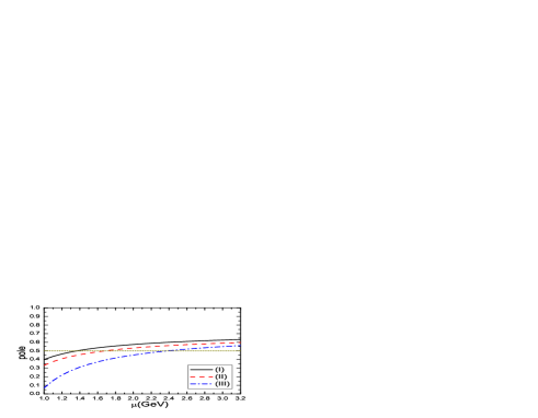
Figure 8: The pole contributions with variations of the energy scales $\mu$ of the QCD spectral densities, where the (I), (II) and (III) correspond to the currents $J_{c\bar{c}}(x)$, $J_{cc}(x)$ and $J_{\mu}^{cc\bar{c}}(x)$, respectively. The central values of the other parameters are chosen.

In Fig.9, we plot the absolute values of the contributions of the vacuum condensates for the central values of the input parameters shown in Table 1 under the condition that the total contributions are normalized to be 1. From the figure, we can see that although the perturbative terms cannot make the dominant contributions, the operator product expansions have very good convergent behaviors. The largest contributions come from the vacuum condensates $\langle\bar{q}q\rangle$, which serve as a milestone, the contributions of the vacuum condensates $D(n)$ decrease quickly with the increase of the dimension $n$ except for some vibrations due to the tiny contributions $D(4)$, $D(7)$ and large contributions $D(6)$. The contributions of the vacuum condensates $\langle\frac{\alpha_{s}GG}{\pi}\rangle$ and $\langle\bar{q}q\rangle\langle\frac{\alpha_{s}GG}{\pi}\rangle$, which are of dimension $4$ and $7$ respectively, play a minor important role. For the currents $J_{c\bar{c}}(x)$ and $J_{\mu}^{cc\bar{c}}(x)$, $|D(6)|>|D(5)|$.

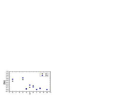
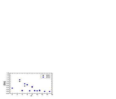
Figure 9: The absolute values of the contributions of the vacuum condensates, where the (I), (II), (III) and (IV) correspond to the currents $J_{c\bar{c}}(x)$, $J_{cc}(x)$, $J_{\mu}^{cc\bar{c}}(x)$ and $J_{\mu}^{ccc}(x)$, respectively. The central values of the other parameters are chosen.

In Fig.10, we plot the predicted masses of the $D^{*}\bar{D}^{*}$, $D^{*}D^{*}$ and $D^{*}D^{*}\bar{D}^{*}$ tetraquark and hexaquark molecular states with variations of the energy scales $\mu$ of the QCD spectral densities, where we have taken the central values of the input parameters. On the other hand, we can rewrite the energy scale formulas as

$$M_{T} = \sqrt{\mu^{2}+4{\mathbb{M}}_{c}^{2}}\,,$$

$$M_{H} = \sqrt{\mu^{2}+9{\mathbb{M}}_{c}^{2}}\,.$$ (25)

If we set ${\mathbb{M}}_{c}=m_{c}=1.84\,\rm{GeV}$, we can obtain the dash-dotted lines $M_{T}=\sqrt{\mu^{2}+4\times(1.84\,\rm{GeV})^{2}}$ and $M_{H}=\sqrt{\mu^{2}+9\times(1.84\,\rm{GeV})^{2}}$ in Fig.10, which intersect with the lines of the masses of the $D^{*}\bar{D}^{*}$, $D^{*}D^{*}$ and $D^{*}D^{*}\bar{D}^{*}$ tetraquark or hexaquark molecular states at the energy scales about $\mu=1.5\,\rm{GeV}$, $1.8\,\rm{GeV}$ and $2.4\,\rm{GeV}$, respectively. In this way, we choose the energy scales of the QCD spectral densities in a consistent way.

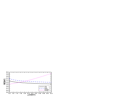
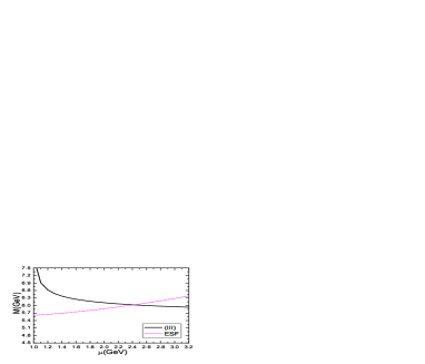
Figure 10: The masses of the tetraquark and hexaquark molecular states with variations of the energy scales $\mu$ of the QCD spectral densities, where the (I), (II) and (III) correspond to the $D^{*}\bar{D}^{*}$, $D^{*}D^{*}$ and $D^{*}D^{*}\bar{D}^{*}$ tetraquark and hexaquark molecular states, respectively, the ESF denotes the formulas $M=\sqrt{\mu^{2}+4\times(1.84\,\rm{GeV})^{2}}$ and $\sqrt{\mu^{2}+9\times(1.84\,\rm{GeV})^{2}}$, respectively.

In this article, we choose the value of the effective $c$-quark mass ${\mathbb{M}}_{c}=1.84\pm 0.01\,\rm{GeV}$ [13], which leads to a uncertainty $\delta\mu=\pm 0.1\,\rm{GeV}$ for the QCD spectral densities. Now we take into account all uncertainties of the input parameters, and obtain the values of the masses and pole residues of the $D^{*}\bar{D}^{*}$, $D^{*}D^{*}$ and $D^{*}D^{*}\bar{D}^{*}$ tetraquark and hexaquark molecular states, which are shown explicitly in Table 2 and Fig.11.

From Fig.11, we can see that there appear flat platforms in the Borel windows for the $D^{*}\bar{D}^{*}$, $D^{*}D^{*}$ and $D^{*}D^{*}\bar{D}^{*}$ molecular states, it is reliable to extract the tetraquark and hexaquark molecular state masses. We can search for the scalar $D^{*}\bar{D}^{*}$, $D^{*}D^{*}$ tetraquark states and the vector $D^{*}D^{*}\bar{D}^{*}$ hexaquark molecular state at the LHCb, Belle II, CEPC, FCC, ILC in the future.

We can take into account the contributions of the intermediate two-meson and three-meson scattering states to the correlation functions $\Pi_{T}(p^{2})$ and $\Pi_{H}(p^{2})$ according to the arguments presented in Refs.[13, 24, 43], as the currents $J_{c\bar{c}}(x)$, $J_{cc}(x)$, $J^{cc\bar{c}}_{\mu}(x)$ and $J^{ccc}_{\mu}(x)$ also couple potentially to the $D^{*}\bar{D}^{*}$, $D^{*}D^{*}$, $D^{*}D^{*}\bar{D}^{*}$ and $D^{*}D^{*}D^{*}$ scattering states respectively according to the standard definition,

$$\langle 0|\bar{q}(0)\gamma_{\alpha}c(0)|D^{*}(p)\rangle = f_{D^{*}}m_{D^{*}}\varepsilon_{\alpha}\,,$$ (26)

where the $\varepsilon_{\alpha}$ is the polarization vector of the $D^{*}$ meson. The renormalized self-energies due to the intermediate meson-loops contribute a finite imaginary part to modify the dispersion relation,

$$\Pi_{T/H}(p^{2}) = -\frac{\lambda_{T/H}^{2}}{p^{2}-M_{T/H}^{2}+i\sqrt{p^{2}}\Gamma_{T/H}(p^{2})}+\cdots\,.$$ (27)

We take into account the finite width effects by the following simple replacement of the hadronic spectral densities,

$$\lambda^{2}_{T/H}\delta\left(s-M^{2}_{T/H}\right) \to \lambda^{2}_{T/H}\frac{1}{\pi}\frac{M_{T/H}\Gamma_{T/H}(s)}{(s-M_{T/H}^{2})^{2}+M_{T/H}^{2}\Gamma_{T/H}^{2}(s)}\,,$$ (28)

then the hadron sides of the QCD sum rules in Eqs.(14)-(15) undergo the following changes,

$$\lambda^{2}_{T/H}\exp\left(-\frac{M^{2}_{Z_{c}}}{T^{2}}\right) \to \lambda^{2}_{T/H}\int_{\Delta^{2}}^{s_{0}}ds\frac{1}{\pi}\frac{M_{T/H}\Gamma_{T/H}(s)}{(s-M_{T/H}^{2})^{2}+M_{T/H}^{2}\Gamma_{T/H}^{2}(s)}\exp\left(-\frac{s}{T^{2}}\right)\,,$$ (29)

$$= \tilde{\lambda}^{2}_{T/H}\exp\left(-\frac{M^{2}_{T/H}}{T^{2}}\right)\,,$$

$$\lambda^{2}_{T/H}M^{2}_{T/H}\exp\left(-\frac{M^{2}_{T/H}}{T^{2}}\right) \to \lambda^{2}_{T/H}\int_{\Delta^{2}}^{s_{0}}ds\,s\,\frac{1}{\pi}\frac{M_{T/H}\Gamma_{T/H}(s)}{(s-M_{T/H}^{2})^{2}+M_{T/H}^{2}\Gamma_{T/H}^{2}(s)}\exp\left(-\frac{s}{T^{2}}\right)\,,$$ (30)

$$= \tilde{\lambda}^{2}_{T/H}M^{2}_{T/H}\exp\left(-\frac{M^{2}_{T/H}}{T^{2}}\right)\,,$$

where the $\Delta^{2}$ are the two-meson or three-meson thresholds. The net effects of the intermediate meson-loops can be absorbed into the pole residues $\tilde{\lambda}_{T/H}$ safely without affecting the predicted tetraquark and hexaquark molecule masses. Even for the $Z_{c}(4200)$, the width is as large as $370^{+70}_{-70}{}^{+70}_{-132}\,\rm{MeV}$, the finite width effects can be safely absorbed into the pole residues [43], so the zero width approximation in the hadronic spectral density works very well.

In Fig.11, we also plot the predicted masses of the $D^{*}D^{*}D^{*}$ hexaquark molecular state with variations of the Borel parameters $T^{2}$ at the energy scales of the QCD spectral densities $\mu=1.0\,\rm{GeV}$, $1.5\,\rm{GeV}$, $2.0\,\rm{GeV}$, $2.5\,\rm{GeV}$ and $3.0\,\rm{GeV}$. From the figure, we can see that there appear no platforms for the $D^{*}D^{*}D^{*}$ hexaquark molecular state. The QCD sum rules do not support the existence of the $D^{*}D^{*}D^{*}$ hexaquark molecular state with the $J^{P}=1^{-}$.

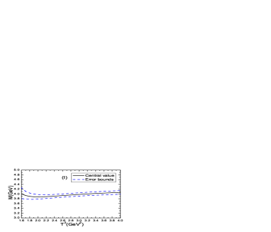
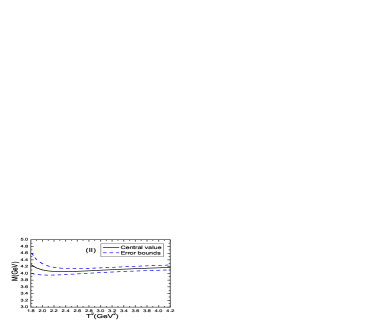
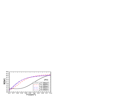
Figure 11: The masses of the tetraquark and hexaquark molecular states with variations of the Borel parameters $T^{2}$, where the (I), (II), (III) and (IV) correspond to the $D^{*}\bar{D}^{*}$, $D^{*}D^{*}$, $D^{*}D^{*}\bar{D}^{*}$ and $D^{*}D^{*}D^{*}$ tetraquark and hexaquark molecular states, respectively.

From Figs.1-2, we can see that compared to the current $J_{c\bar{c}}(x)$, there are connected (nonfactorizable) Feynman diagrams in the correlation function $\Pi(p)$ for the current $J_{cc}(x)$ besides the disconnected (factorizable) Feynman diagrams. The connected diagrams and other diagrams obtained by substituting the quark lines with other terms in the full light and heavy propagators lead to more stable QCD sum rules for the predicted mass of the $D^{*}D^{*}$ tetraquark molecular state, see Fig.11. From Figs.3-5, we can see that compared to the current $J_{cc\bar{c}}(x)$, there are connected Feynman diagrams in the correlation function $\Pi_{\mu\nu}(p)$ for the current $J_{ccc}(x)$ besides the disconnected Feynman diagrams. The contributions from the connected diagrams and other diagrams obtained by substituting the quark lines with other terms in the full light and heavy propagators are so large as to make the QCD sum rules for the mass of the $D^{*}D^{*}D^{*}$ hexaquark molecular state unstable, see Fig.11.

In summary, the connected Feynman diagrams at the tree level shown in Fig.2 and their induced diagrams via substituting the quark lines make positive contributions, the connected Feynman diagrams at the tree level shown in Fig.5 and their induced diagrams via substituting the quark lines make negative or destructive contributions, which are in contrast to the assertion of Lucha, Melikhov and Sazdjian that the factorizable (disconnected) diagrams in the color space only make contributions to the meson-meson scattering states, the tetraquark molecular states begin to receive contributions from the nonfactorizable (connected) diagrams at the order $\mathcal{O}(\alpha_{s}^{2})$ [11, 12]. In fact, it is of no use to distinguish the factorizable and nonfactorizable properties of the Feynman diagrams in the color space.

In Fig.12, we plot the contributions of the vacuum condensates $D(n)$ with $n\geq 8$ for the $J_{\mu}^{cc\bar{c}}(x)$ and $J_{\mu}^{ccc}(x)$ with the central values of the input parameters shown in Table 1. From the figure, we can see that, for the current $J_{\mu}^{cc\bar{c}}(x)$, the contributions of the higher dimensional vacuum condensates are huge for the small Borel parameters $T^{2}$, and decrease monotonously and quickly with the increase of the Borel parameters $T^{2}$ at the region $T^{2}\leq 3.6\,\rm{GeV}^{2}$, then they decrease monotonously and slowly with the increase of the Borel parameters $T^{2}$. The higher dimensional vacuum condensates play a minor important role in the Borel windows, but they play a very important role in determining the Borel windows or in warranting the appearances of the Borel platforms. While for the current $J_{\mu}^{ccc}(x)$, the contributions of the higher dimensional vacuum condensates are not greatly amplified for the small Borel parameters $T^{2}$, and decrease monotonously and slowly with the increase of the Borel parameters $T^{2}$, which cannot stabilize the QCD sum rules to obtain reliable predictions, the QCD sum rules at the hadron side may be dominated by the three-meson scattering states.

$J^{P}$	$T^{2}(\rm{GeV}^{2})$	$\sqrt{s_{0}}(\rm{GeV})$	$\mu(\rm{GeV})$	pole
$0^{+}(D^{*}\bar{D}^{*})$	$2.8-3.2$	$4.55\pm 0.10$	$1.5$	$(41-64)\%$
$0^{+}(D^{*}D^{*})$	$3.0-3.4$	$4.65\pm 0.10$	$1.8$	$(41-62)\%$
$1^{-}(D^{*}D^{*}\bar{D}^{*})$	$3.9-4.3$	$6.60\pm 0.10$	$2.4$	$(41-60)\%$
$1^{-}(D^{*}D^{*}D^{*})$	$3.9-4.3$	$6.60\pm 0.10$	$2.4$	$(39-60)\%$

Table 1: The Borel parameters, continuum threshold parameters, energy scales of the QCD spectral densities and pole contributions for the $D^{*}\bar{D}^{*}$, $D^{*}D^{*}$, $D^{*}D^{*}\bar{D}^{*}$ and $D^{*}D^{*}D^{*}$ tetraquark and hexaquark molecular states.

$J^{P}$	$M_{T/H}$	$\lambda_{T/H}$
$0^{+}(D^{*}\bar{D}^{*})$	$3.98\pm 0.09\,\rm{GeV}$	$(4.05\pm 0.70)\times 10^{-2}\rm{GeV}^{5}$
$0^{+}(D^{*}D^{*})$	$4.11\pm 0.09\,\rm{GeV}$	$(8.36\pm 1.32)\times 10^{-2}\rm{GeV}^{5}$
$1^{-}(D^{*}D^{*}\bar{D}^{*})$	$6.03\pm 0.11\,\rm{GeV}$	$(3.14\pm 0.55)\times 10^{-3}\rm{GeV}^{8}$

Table 2: The masses and pole residues for the $D^{*}\bar{D}^{*}$, $D^{*}D^{*}$ and $D^{*}D^{*}\bar{D}^{*}$ tetraquark and hexaquark molecular states.

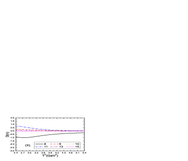
Figure 12: The contributions of the higher dimensional vacuum condensates with variations of the Borel parameters $T^{2}$ for the central values of other parameters, where the (I) and (II) correspond to the currents $J_{\mu}^{cc\bar{c}}(x)$ and $J_{\mu}^{ccc}(x)$, respectively.

4 Conclusion

In this article, we construct the color-singlet-color-singlet type currents and the color-singlet-color-singlet-color-singlet type currents to interpolate the scalar $D^{*}\bar{D}^{*}$, $D^{*}D^{*}$ tetraquark molecular states and the vector $D^{*}D^{*}\bar{D}^{*}$, $D^{*}D^{*}D^{*}$ hexaquark molecular states, respectively, and study their masses and pole residues with the QCD sum rules in details by carrying out the operator product expansion up to the vacuum condensates of dimension 10 and dimension 15, respectively. In calculations, we choose the pertinent energy scales of the QCD spectral densities with the energy scale formula $\mu=\sqrt{M^{2}_{T}-(2{\mathbb{M}}_{c})^{2}}$ and $\sqrt{M^{2}_{H}-(3{\mathbb{M}}_{c})^{2}}$ for the tetraquark molecular states and hexaquark molecular states respectively in a consistent way, which can enhance the pole contributions remarkably and also improve the convergent behaviors of the operator product expansion remarkably. We obtain stable QCD sum rules for the masses and pole residues of the scalar $D^{*}\bar{D}^{*}$, $D^{*}D^{*}$ tetraquark molecular states and the vector $D^{*}D^{*}\bar{D}^{*}$ hexaquark molecular state, but cannot obtain stable QCD sum rules for the vector $D^{*}D^{*}D^{*}$ hexaquark molecular state. We can search for the $D^{*}\bar{D}^{*}$, $D^{*}D^{*}$ and $D^{*}D^{*}\bar{D}^{*}$ tetraquark and hexaquark molecular states at the LHCb, Belle II, CEPC, FCC, ILC in the future. In calculations, we observe that the connected Feynman diagrams at the tree level and their induced diagrams via substituting the quark lines make positive contributions in the QCD sum rules for the $D^{*}D^{*}$ tetraquark molecular state, but make negative or destructive contributions in the QCD sum rules for the $D^{*}D^{*}D^{*}$ hexaquark molecular state, where the tree level denotes the lowest order contributions shown in Figs.1-5. Lucha, Melikhov and Sazdjian assert that those nonfactorizable Feynman diagrams shown in Fig.2 and Fig.5 can be deformed into the box diagrams. It is unfeasible, those nonfactorizable Feynman diagrams can only be deformed into the box diagrams in the color space, not in the momentum space. It is of no use or meaningless to distinguish the factorizable and nonfactorizable properties of the Feynman diagrams in the color space in the operator product expansion so as to interpret them in terms of the hadronic observables, we can only obtain information about the short-distance and long-distance contributions.

Appendix

The explicit expressions of the QCD spectral densities $\rho^{c\bar{c}}_{T}(s,\mu)$ and $\rho^{cc}_{T}(s,\mu)$,

$$\rho^{c\bar{c}}_{T}(s,\mu) = \frac{3}{512\pi^{6}}\int dydz\,yz\left(1-y-z\right)^{2}\left(s-\overline{m}_{c}^{2}\right)^{3}\left(3s-\overline{m}_{c}^{2}\right)$$ (31)

$$-\frac{3m_{c}\langle\bar{q}q\rangle}{16\pi^{4}}\int dydz\,y\left(1-y-z\right)\left(s-\overline{m}_{c}^{2}\right)\left(2s-\overline{m}_{c}^{2}\right)$$

$$+\frac{m_{c}\langle\bar{q}g_{s}\sigma Gq\rangle}{64\pi^{4}}\int dydz\,y\left(7s-6\overline{m}_{c}^{2}\right)+\frac{m_{c}^{2}\langle\bar{q}q\rangle^{2}}{4\pi^{2}}\int dy\,$$

$$-\frac{m_{c}^{2}\langle\bar{q}q\rangle\langle\bar{q}g_{s}\sigma Gq\rangle}{8\pi^{2}}\int dy\,\left(1+\frac{s}{T^{2}}\right)\delta\left(s-\widetilde{m}_{c}^{2}\right)$$

$$+\frac{m_{c}^{2}\langle\bar{q}g_{s}\sigma Gq\rangle^{2}}{64\pi^{2}T^{6}}\int dy\,s^{2}\delta\left(s-\widetilde{m}_{c}^{2}\right)$$

$$-\frac{m_{c}^{2}}{128\pi^{4}}\langle\frac{\alpha_{s}GG}{\pi}\rangle\int dydz\,\frac{z(1-y-z)^{2}}{y^{2}}\left(3s-2\overline{m}_{c}^{2}\right)$$

$$+\frac{m_{c}^{3}\langle\bar{q}q\rangle}{96\pi^{2}}\langle\frac{\alpha_{s}GG}{\pi}\rangle\int dydz\,\left(1+\frac{z}{y}\right)\frac{(1-y-z)}{y^{2}}\left(1+\frac{s}{T^{2}}\right)\delta\left(s-\overline{m}_{c}^{2}\right)$$

$$+\frac{m_{c}\langle\bar{q}q\rangle}{32\pi^{2}}\langle\frac{\alpha_{s}GG}{\pi}\rangle\int dydz\,\left[1-\frac{z(1-y-z)}{y^{2}}\right]\left[2+s\,\delta\left(s-\overline{m}_{c}^{2}\right)\right]$$

$$-\frac{m_{c}^{4}\langle\bar{q}q\rangle^{2}}{36T^{4}}\langle\frac{\alpha_{s}GG}{\pi}\rangle\int dy\,\frac{1}{y^{3}}\delta\left(s-\widetilde{m}_{c}^{2}\right)+\frac{m_{c}^{2}\langle\bar{q}q\rangle^{2}}{72T^{6}}\int dy\,s^{2}\delta\left(s-\widetilde{m}_{c}^{2}\right)$$

$$+\frac{m_{c}^{2}\langle\bar{q}q\rangle^{2}}{12T^{2}}\langle\frac{\alpha_{s}GG}{\pi}\rangle\int dy\,\frac{1}{y^{2}}\delta\left(s-\widetilde{m}_{c}^{2}\right)+\frac{\langle\bar{q}g_{s}\sigma Gq\rangle^{2}}{256\pi^{2}T^{2}}\int dy\,s\delta\left(s-\widetilde{m}_{c}^{2}\right)$$

$$-\frac{m_{c}\langle\bar{q}q\rangle}{192\pi^{2}}\langle\frac{\alpha_{s}GG}{\pi}\rangle\int dy\,y\left[2+s\delta\left(s-\widetilde{m}_{c}^{2}\right)\right]\,,$$

$$\rho^{cc}_{T}(s,\mu) = \frac{7}{512\pi^{6}}\int dydz\,yz\left(1-y-z\right)^{2}\left(s-\overline{m}_{c}^{2}\right)^{3}\left(3s-\overline{m}_{c}^{2}\right)$$

$$-\frac{m_{c}^{2}}{512\pi^{6}}\int dydz\left(1-y-z\right)^{2}\left(s-\overline{m}_{c}^{2}\right)^{3}$$

$$-\frac{m_{c}\langle\bar{q}q\rangle}{2\pi^{4}}\int dydz\,y\left(1-y-z\right)\left(s-\overline{m}_{c}^{2}\right)\left(2s-\overline{m}_{c}^{2}\right)$$

$$+\frac{m_{c}\langle\bar{q}g_{s}\sigma Gq\rangle}{8\pi^{4}}\int dydz\,y\left(3s-2\overline{m}_{c}^{2}\right)$$

$$-\frac{\langle\bar{q}q\rangle^{2}}{24\pi^{2}}\int dy\,y(1-y)\left(3s-2\widetilde{m}_{c}^{2}\right)+\frac{7m_{c}^{2}\langle\bar{q}q\rangle^{2}}{12\pi^{2}}\int dy\,$$

$$+\frac{\langle\bar{q}q\rangle\langle\bar{q}g_{s}\sigma Gq\rangle}{48\pi^{2}}\int dy\,y(1-y)\left[6+\left(4s+\frac{s^{2}}{T^{2}}\right)\delta\left(s-\widetilde{m}_{c}^{2}\right)\right]$$

$$-\frac{7m_{c}^{2}\langle\bar{q}q\rangle\langle\bar{q}g_{s}\sigma Gq\rangle}{24\pi^{2}}\int dy\,\left(1+\frac{s}{T^{2}}\right)\delta\left(s-\widetilde{m}_{c}^{2}\right)$$

$$-\frac{\langle\bar{q}g_{s}\sigma Gq\rangle^{2}}{384\pi^{2}}\int dy\,y(1-y)\left(6+\frac{6s}{T^{2}}+\frac{3s^{2}}{T^{4}}+\frac{s^{3}}{T^{6}}\right)\delta(s-\widetilde{m}_{c}^{2})$$

$$+\frac{7m_{c}^{2}\langle\bar{q}g_{s}\sigma Gq\rangle^{2}}{192\pi^{2}T^{6}}\int dy\,s^{2}\delta\left(s-\widetilde{m}_{c}^{2}\right)$$

$$-\frac{7m_{c}^{2}}{384\pi^{4}}\langle\frac{\alpha_{s}GG}{\pi}\rangle\int dydz\,\frac{z(1-y-z)^{2}}{y^{2}}\left(3s-2\overline{m}_{c}^{2}\right)$$

$$+\frac{m_{c}^{4}}{768\pi^{4}}\langle\frac{\alpha_{s}GG}{\pi}\rangle\int dydz\,\frac{(1-y-z)^{2}}{y^{3}}$$

$$+\frac{m_{c}^{3}\langle\bar{q}q\rangle}{36\pi^{2}}\langle\frac{\alpha_{s}GG}{\pi}\rangle\int dydz\,\left(1+\frac{z}{y}\right)\frac{1-y-z}{y^{2}}\left(1+\frac{s}{T^{2}}\right)\delta(s-\overline{m}_{c}^{2})$$

$$+\frac{m_{c}^{2}\langle\bar{q}q\rangle^{2}}{216T^{4}}\langle\frac{\alpha_{s}GG}{\pi}\rangle\int dy\,\frac{1-y}{y^{2}}s\,\delta\left(s-\widetilde{m}_{c}^{2}\right)$$

$$-\frac{7m_{c}^{4}\langle\bar{q}q\rangle^{2}}{108T^{4}}\langle\frac{\alpha_{s}GG}{\pi}\rangle\int dy\,\frac{1}{y^{3}}\delta\left(s-\widetilde{m}_{c}^{2}\right)$$

$$-\frac{m_{c}^{2}}{256\pi^{4}}\langle\frac{\alpha_{s}GG}{\pi}\rangle\int dydz\,\frac{(1-y-z)^{2}}{y^{2}}\left(s-\overline{m}_{c}^{2}\right)$$

$$+\frac{m_{c}\langle\bar{q}q\rangle}{48\pi^{2}}\langle\frac{\alpha_{s}GG}{\pi}\rangle\int dydz\,\left[4-\frac{4z(1-y-z)}{y^{2}}+\frac{1-y-z}{z}-\frac{z}{y}\right]\left[2+s\delta\left(s-\overline{m}_{c}^{2}\right)\right]$$

$$+\frac{7m_{c}^{2}\langle\bar{q}q\rangle^{2}}{36T^{2}}\langle\frac{\alpha_{s}GG}{\pi}\rangle\int dy\,\frac{1}{y^{2}}\delta\left(s-\widetilde{m}_{c}^{2}\right)$$

$$-\frac{1}{128\pi^{4}}\langle\frac{\alpha_{s}GG}{\pi}\rangle\int dydz\,yz\left(s-\overline{m}_{c}^{2}\right)\left(2s-\overline{m}_{c}^{2}\right)$$

$$-\frac{m_{c}^{2}}{256\pi^{4}}\langle\frac{\alpha_{s}GG}{\pi}\rangle\int dydz\,\frac{4-3y-4z}{y}\left(s-\overline{m}_{c}^{2}\right)$$

$$-\frac{1}{256\pi^{4}}\langle\frac{\alpha_{s}GG}{\pi}\rangle\int dydz\,(1-y-z)^{2}\left(s-\overline{m}_{c}^{2}\right)\left(2s-\overline{m}_{c}^{2}\right)$$

$$-\frac{\langle\bar{q}q\rangle^{2}}{144}\langle\frac{\alpha_{s}GG}{\pi}\rangle\int dy\,\left(1+\frac{5s}{T^{2}}\right)\delta\left(s-\widetilde{m}_{c}^{2}\right)$$

$$-\frac{m_{c}\langle\bar{q}g_{s}\sigma Gq\rangle}{32\pi^{4}}\int dydz\,\left(1-2y-z\right)\left(3s-2\overline{m}_{c}^{2}\right)$$

$$-\frac{\langle\bar{q}q\rangle\langle\bar{q}g_{s}\sigma Gq\rangle}{24\pi^{2}}\int dy\,\left(1-y\right)\left[2+s\,\delta\left(s-\widetilde{m}_{c}^{2}\right)\right]$$

$$+\frac{\langle\bar{q}g_{s}\sigma Gq\rangle^{2}}{96\pi^{2}}\int dy\,\left(1-y\right)\left(2+\frac{2s}{T^{2}}+\frac{s^{2}}{T^{4}}\right)\delta\left(s-\widetilde{m}_{c}^{2}\right)$$

$$-\frac{\langle\bar{q}g_{s}\sigma Gq\rangle^{2}}{192\pi^{2}}\int dy\,\left(1+\frac{s}{T^{2}}\right)\delta\left(s-\widetilde{m}_{c}^{2}\right)+\frac{\langle\bar{q}g_{s}\sigma Gq\rangle^{2}}{128\pi^{2}T^{2}}\int dy\,s\,\delta\left(s-\widetilde{m}_{c}^{2}\right)$$

$$-\frac{m_{c}\langle\bar{q}q\rangle}{72\pi^{2}}\langle\frac{\alpha_{s}GG}{\pi}\rangle\int dy\,y\left[2+s\,\delta\left(s-\widetilde{m}_{c}^{2}\right)\right]$$

$$-\frac{\langle\bar{q}q\rangle^{2}}{432}\langle\frac{\alpha_{s}GG}{\pi}\rangle\int dy\,y(1-y)\left(6+\frac{6s}{T^{2}}+\frac{3s^{2}}{T^{4}}+\frac{s^{3}}{T^{6}}\right)\delta\left(s-\widetilde{m}_{c}^{2}\right)$$

$$+\frac{7m_{c}^{2}\langle\bar{q}q\rangle^{2}}{216T^{6}}\langle\frac{\alpha_{s}GG}{\pi}\rangle\int dy\,s^{2}\delta\left(s-\widetilde{m}_{c}^{2}\right)\,,$$ (32)

where $\int dydz=\int_{y_{i}}^{y_{f}}dy\int_{z_{i}}^{1-y}dz$, $\int dy=\int_{y_{i}}^{y_{f}}dy$, $y_{f}=\frac{1+\sqrt{1-4m_{c}^{2}/s}}{2}$, $y_{i}=\frac{1-\sqrt{1-4m_{c}^{2}/s}}{2}$, $z_{i}=\frac{ym_{c}^{2}}{ys-m_{c}^{2}}$, $\overline{m}_{c}^{2}=\frac{(y+z)m_{c}^{2}}{yz}$, $\widetilde{m}_{c}2=\frac{m_{c}^{2}}{y(1-y)}$, $\int_{y_{i}}^{y_{f}}dy\to\int_{0}^{1}dy$, $\int_{z_{i}}^{1-y}dz\to\int_{0}^{1-y}dz$ when the $\delta$ functions $\delta\left(s-\overline{m}_{c}^{2}\right)$ and $\delta\left(s-\widetilde{m}_{c}^{2}\right)$ appear.

References

• [1] M. A. Shifman, A. I. Vainshtein and V. I. Zakharov, Nucl. Phys. B147 (1979) 385; Nucl. Phys. B147 (1979) 448.
• [2] L. J. Reinders, H. Rubinstein and S. Yazaki, Phys. Rept. 127 (1985) 1.
• [3] P. Colangelo and A. Khodjamirian, hep-ph/0010175.
• [4] S. K. Choi et al, Phys. Rev. Lett. 91 (2003) 262001.
• [5] R. D. Matheus, S. Narison, M. Nielsen and J. M. Richard, Phys. Rev. D75 (2007) 014005.
• [6] R. M. Albuquerque, J. M. Dias, K. P. Khemchandani, A. M. Torres, F. S. Navarra, M. Nielsen and C. M. Zanetti, J. Phys. G46 (2019) 093002.
• [7] S. H. Lee, A. Mihara, F. S. Navarra and M. Nielsen, Phys. Lett. B661 (2008) 28; Z. G. Wang, Z. C. Liu and X. H. Zhang, Eur. Phys. J. C64 (2009) 373; J. R. Zhang and M. Q. Huang, Commun. Theor. Phys. 54 (2010) 1075; J. R. Zhang, Phys. Rev. D87 (2013) 116004.
• [8] Z. G. Wang and T. Huang, Eur. Phys. J. C74 (2014) 2891; Z. G. Wang, Eur. Phys. J. C74 (2014) 2963.
• [9] S. H. Lee and K. Morita and M. Nielsen, Phys. Rev. D78 (2008) 076001; K. Azizi, Y. Sarac and H. Sundu, Phys. Lett. B782 (2018) 694; Z. G. Wang and X. Wang, Chin. Phys. C44 (2020) 103102.
• [10] H. X. Chen, W. Chen, X. Liu, T. G. Steele and S. L. Zhu, Phys. Rev. Lett. 115 (2015) 172001; K. Azizi, Y. Sarac and H. Sundu, Phys. Rev. D95 (2017) 094016; Z. G. Wang, Int. J. Mod. Phys. A34 (2019) 1950097.
• [11] W. Lucha, D. Melikhov and H. Sazdjian, Phys. Rev. D100 (2019) 014010.
• [12] W. Lucha, D. Melikhov and H. Sazdjian, Phys. Rev. D100 (2019) 074029.
• [13] Z. G. Wang, Phys. Rev. D101 (2020) 074011.
• [14] H. J. Lee and N. I. Kochelev, Phys. Rev. D78 (2008) 076005.
• [15] X. L. Ren, B. B. Malabarba, L. S. Geng, K. P. Khemchandani and A. M. Torres, Phys. Lett. B785 (2018) 112.
• [16] M. P. Valderrama, Phys. Rev. D98 (2018) 034017.
• [17] J. M. Dias, V. R. Debastiani, L. Roca, S. Sakai and E. Oset, Phys. Rev. D96 (2017) 094007.
• [18] J. M. Dias, L. Roca and S. Sakai, Phys. Rev. D97 (2018) 056019.
• [19] Z. Y. Di and Z. G. Wang, Adv. High Energy Phys. 2019 (2019) 8958079.
• [20] K. P. Khemchandani, A. Martinez Torres, M. Nielsen and F. S. Navarra, Phys. Rev. D89 (2014) 014029.
• [21] C. Y. Cui, Y. L. Liu and M. Q. Huang, Eur. Phys. J. C73 (2013) 2661.
• [22] J. R. Zhang and M. Q. Huang, Phys. Rev. D80 (2009) 056004.
• [23] R. Albuquerque, S. Narison, F. Fanomezana, A. Rabemananjara, D. Rabetiarivony and G. Randriamanatrika, Int. J. Mod. Phys. A31 (2016) 1650196.
• [24] Z. G. Wang and T. Huang, Phys. Rev. D89 (2014) 054019.
• [25] P. Pascual and R. Tarrach, “QCD: Renormalization for the practitioner”, Springer Berlin Heidelberg (1984).
• [26] D. B. Leinweber, Annals Phys. 254 (1997) 328; and references therein.
• [27] S. Narison, Phys. Lett. B673 (2009) 30.
• [28] V. A. Novikov, M. A. Shifman, A. I. Vainshtein, M. B. Voloshin and V. I. Zakharov, Nucl. Phys. B237 (1984) 525.
• [29] P. Gubler and D. Satow, Prog. Part. Nucl. Phys. 106 (2019) 1.
• [30] W. Lucha, D. Melikhov and S. Simula, Phys. Lett. B701 (2011) 82.
• [31] Z. G. Wang, Eur. Phys. J. C74 (2014) 2874.
• [32] Z. G. Wang, Commun. Theor. Phys. 63 (2015) 466; Z. G. Wang and Y. F. Tian, Int. J. Mod. Phys. A30 (2015) 1550004.
• [33] Z. G. Wang, Int. J. Mod. Phys. A35 (2020) 2050003.
• [34] Z. G. Wang, Phys. Rev. D102 (2020) 034008.
• [35] Z. G. Wang, Int. J. Mod. Phys. A35 (2020) 2050073.
• [36] Z. G. Wang, AAPPS Bulletin 31 (2021) 5.
• [37] M. Tanabashi et al, Phys. Rev. D98 (2018) 030001.
• [38] S. Narison and R. Tarrach, Phys. Lett. 125 B (1983) 217.
• [39] E. J. Eichten and C. Quigg, Phys. Rev. D99 (2019) 054025.
• [40] Z. G. Wang, Chin. Phys. C41 (2017) 083103.
• [41] Z. G. Wang, Phys. Rev. D83 (2011) 014009; Z. G. Wang, Phys. Rev. D88 (2013) 114003.
• [42] Z. G. Wang, Eur. Phys. J. C75 (2015) 427.
• [43] Z. G. Wang, Int. J. Mod. Phys. A30 (2015) 1550168.