FTT-NAS: Discovering Fault-Tolerant Convolutional Neural Architecture
Abstract.
With the fast evolvement of embedded deep-learning computing systems, applications powered by deep learning are moving from the cloud to the edge. When deploying neural networks (NNs) onto the devices under complex environments, there are various types of possible faults: soft errors caused by cosmic radiation and radioactive impurities, voltage instability, aging, temperature variations, malicious attackers, etc. Thus the safety risk of deploying NNs is now drawing much attention. In this paper, after the analysis of the possible faults in various types of NN accelerators, we formalize and implement various fault models from the algorithmic perspective. We propose Fault-Tolerant Neural Architecture Search (FT-NAS) to automatically discover convolutional neural network (CNN) architectures that are reliable to various faults in nowadays devices. Then we incorporate fault-tolerant training (FTT) in the search process to achieve better results, which is referred to as FTT-NAS. Experiments on CIFAR-10 show that the discovered architectures outperform other manually designed baseline architectures significantly, with comparable or fewer floating-point operations (FLOPs) and parameters. Specifically, with the same fault settings, F-FTT-Net discovered under the feature fault model achieves an accuracy of 86.2% (VS. 68.1% achieved by MobileNet-V2), and W-FTT-Net discovered under the weight fault model achieves an accuracy of 69.6% (VS. 60.8% achieved by ResNet-18). By inspecting the discovered architectures, we find that the operation primitives, the weight quantization range, the capacity of the model, and the connection pattern have influences on the fault resilience capability of NN models.
1. Introduction
Convolutional Neural Networks (CNNs) have achieved breakthroughs in various tasks, including classification (He et al., 2016), detection (Liu et al., 2016) and segmentation (Long et al., 2015), etc. Due to their promising performance, CNNs have been utilized in various safety-critic applications, such as autonomous driving, intelligent surveillance, and identification. Meanwhile, driven by the recent academic and industrial efforts, the neural network accelerators based on various hardware platforms (e.g., Application Specific Integrated Circuits (ASIC) (Chen et al., 2014), Field Programmable Gate Array (FPGA) (Qiu et al., 2016), Resistive Random-Access Memory (RRAM) (Chi et al., 2016)) have been rapidly evolving.
The robustness and reliability related issues of deploying neural networks onto various embedded devices for safety-critical applications are attracting more and more attention. There is a large stream of algorithmic studies on various robustness-related characteristics of NNs, e.g., adversarial robustness (Szegedy et al., 2013), data poisoning (Shafahi et al., 2018), interpretability (Zhang et al., 2018), and so on. However, no hardware models are taken into consideration in these studies. Besides the issues from the purely algorithmic perspective, there exist hardware-related reliability issues when deploying NNs onto nowadays embedded devices. With the down-scaling of CMOS technology, circuits become more sensitive to cosmic radiation and radioactive impurities (Henkel et al., 2013). Voltage instability, aging, and temperature variations are also common effects that could lead to errors. As for the emerging metal-oxide RRAM devices, due to the immature technology, they suffer from many types of device faults (Chen et al., 2015), among which hard faults such as Stuck-at-Faults (SAFs) damage the computing accuracy severely and could not be easily mitigated (Xia et al., 2018). Moreover, malicious attackers can attack the edge devices by embedding hardware Trojans, manipulating back-doors, and doing memory injection (Zhao et al., 2019).
Recently, some studies (Liu et al., 2017; Vialatte and Leduc-Primeau, 2017; Schorn et al., 2018) analyzed the sensitivity of NN models. They proposed to predict whether a layer or a neuron is sensitive to faults and protect the sensitive ones. For fault tolerance, a straightforward way is to introduce redundancy in the hardware. Triple Modular Redundancy (TMR) is a commonly used but expensive method to tolerate a single fault (Bolchini et al., 2007; She and Li, 2017; Zhao et al., 2018). Studies (Xia et al., 2018; Liu et al., 2017) proposed various redundancy schemes for Stuck-at-Faults tolerance in the RRAM-based Computing Systems. For increasing the algorithmic fault resilience capability, studies (He et al., 2019; Hacene et al., 2019) proposed to use fault-tolerant training (FTT), in which random faults are injected in the training process.
Although redesigning the hardware for reliability is effective, it is not flexible and inevitably introduces a large overhead. It would be better if the issues could be mitigated as far as possible from the algorithmic perspective. Existing methods mainly concerned about designing training methods and analyzing the weight distribution (Schorn et al., 2018; He et al., 2019; Hacene et al., 2019). Intuitively, the neural architecture might also be important for the fault tolerance characteristics (Arechiga and Michaels, 2018; Li et al., 2017), since it determines the “path” of fault propagation. To verify these intuitions, the accuracies of baselines under a random bit-bias feature fault model111The random bit-bias feature fault model is formalized in Sec. 3.4. are shown in Table 1, and the results under SAF weight fault model222The SAF weight fault model is formalized in Sec. 3.5. are shown in Table 2. These preliminary experiments on the CIFAR-10 dataset show that the fault tolerance characteristics vary among neural architectures, which motivates the employment of neural architecture search (NAS) techniques in designing fault-tolerant neural architectures. We emphasize that our work is orthogonal to most of the previous methods based on hardware or mapping strategy design. To our best knowledge, our work is the first to increase the algorithmic fault resilience capability by optimizing the NN architecture.
| Model | Acc() | #Params | #FLOPs |
|---|---|---|---|
| ResNet-18 | 94.7/63.4/10.0 | 11.2M | 1110M |
| VGG-16† | 93.1/21.4/10.0 | 14.7M | 626M |
| MobileNet-V2 | 92.3/10.0/10.0 | 2.3M | 182M |
: For simplicity, we only keep one fully-connected layer of VGG-16.
| Model | Acc(0/4%/8%) | #Params | #FLOPs |
|---|---|---|---|
| ResNet-18 | 94.7/64.8/17.8 | 11.2M | 1110M |
| VGG-16 | 93.1/45.7/14.3 | 14.7M | 626M |
| MobileNet-V2 | 92.3/26.2/11.7 | 2.3M | 182M |
In this paper, we employ NAS to discover fault-tolerant neural network architectures against feature faults and weight faults, and demonstrate the effectiveness by experiments. The main contributions of this paper are as follows.
-
•
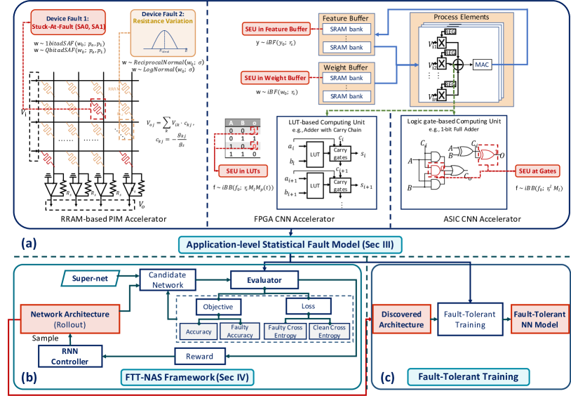
We analyze the possible faults in various types of NN accelerators (ASIC-based, FPGA-based, and RRAM-based), and formalize the statistical fault models from the algorithmic perspective. After the analysis, we adopt the Multiply-Accumulate (MAC)-i.i.d Bit-Bias (MiBB) model and the arbitrary-distributed Stuck-at-Fault (adSAF) model in the neural architecture search for tolerating feature faults and weight faults, respectively.
-
•
We establish a multi-objective neural architecture search framework. On top of this framework, we propose two methods to discover neural architectures with better reliability: FT-NAS (NAS with a fault-tolerant multi-objective), and FTT-NAS (NAS with a fault-tolerant multi-objective and fault-tolerant training (FTT)).
-
•
We employ FT-NAS and FTT-NAS to discover architectures for tolerating feature faults and weight faults. The discovered architectures, F-FTT-Net and W-FTT-Net have comparable or fewer floating-point operations (FLOPs) and parameters, and achieve better fault resilience capabilities than the baselines. With the same fault settings, F-FTT-Net discovered under the feature fault model achieves an accuracy of 86.2% (VS. 68.1% achieved by MobileNet-V2), and W-FTT-Net discovered under the weight fault model achieves an accuracy of 69.6% (VS. 60.8% achieved by ResNet-18). The ability of W-FTT-Net to defend against several other types of weight faults is also illustrated by experiments.
-
•
We analyze the discovered architectures, and discuss how the weight quantization range, the capacity of the model, and the connection pattern influence the fault resilience capability of a neural network.
The rest of this paper is organized as follows. The related studies and the preliminaries are introduced in Section 2. In Section 3, we conduct comprehensive analysis on the possible faults and formalize the fault models. In Section 4, we elaborate on the design of the fault-tolerant NAS system. Then in Section 5, the effectiveness of our method is illustrated by experiments, and the insights are also presented. Finally, we discuss and conclude our work in Section 6 and Section 7.
2. Related work and preliminary
2.1. Convolutional Neural Network
Usually, a convolutional neural network is constructed by stacking multiple convolution layers and optional pooling layers, followed by fully-connected layers. Denoting the input feature map (IFM), before-activation output feature map, output feature map (OFM, i.e. activations), weights and bias of -th convolution layer as , , , , , the computation can be written as:
| (1) | ||||
where is the convolution operator, is the activation function, for which the ReLU function () is the commonest choice. From now on, we omit the superscript for simplicity.
2.2. NN Accelerators and Fixed-point Arithmetic
With dedicated data flow design for efficient neural network processing, FPGA-based NN accelerators could achieve at least 10x better energy efficiency than GPUs (Qiu et al., 2016; Guo et al., 2019). And ASIC-based accelerators could achieve even higher efficiency (Chen et al., 2014). Besides, RRAM-based computing systems are promising solutions for energy-efficient brain-inspired computing (Chi et al., 2016), due to their capability of performing matrix-vector-multiplications (MVMs) in memory. Existing studies have shown RRAM-based Processing-In-Memory (PIM) architectures can enhance the energy efficiency by over compared with both GPU and ASIC solutions, as they can eliminate the large data movements of bandwidth-bounded NN applications (Chi et al., 2016). For the detailed and formal hardware architecture descriptions, we refer the readers to the references listed above.
Currently, fixed-point arithmetic units are implemented by most of the NN accelerators, as 1) they consume much fewer resources and are much more efficient than the floating-point ones (Guo et al., 2019); 2) NN models are proven to be insensitive to quantization (Qiu et al., 2016; Hubara et al., 2017). Consequently, quantization is usually applied before a neural network model is deployed onto the edge devices. To keep consistent with the actual deploying scenario, our simulation incorporates 8-bit dynamic fixed-point quantization for the weights and activations. More specifically, independent step sizes are used for the weights and activations of different layers. Denoting the fraction length and bit-width of a tensor as and , the step size (resolution) of the representation is . For common CMOS platforms, in which complement representation is used for numbers, the representation range of both weights and features is
| (2) |
As for RRAM-based NN platforms, two separate crossbars are usually used for storing positive and negative weights (Chi et al., 2016). Thus the representation range of the weights (denoted by the superscript) is
| (3) |
For the feature representation in RRAM-based platforms, by assuming that the Analog to Digital Converters (ADCs) and Digital to Analog Converters (DACs) have enough precision, and the CMOS bit-width is -bit, the representation range of features (denoted by the superscript) in CMOS circuits is
| (4) |
2.3. Fault Resilience for CMOS-based Accelerators
Henkel et al. (2013); Borkar (2005); Slayman (2011) revealed that advanced nanotechnology makes circuits more vulnerable to soft errors. Unlike hard errors, soft errors do not damage the underlying circuits, but instead trigger an upset of the logic state. The dominant cause of soft errors in CMOS circuits is the radioactive events, in which a single particle strikes an electronic device. Arechiga and Michaels (2018); Libano et al. (2019) explored how the Single-Event Upset (SEU) faults impact the FPGA-based CNN computation system.
TMR is a commonly used approach to mitigate SEUs (Bolchini et al., 2007; She and Li, 2017; Zhao et al., 2018). Traditional TMR methods are agnostic of the NN applications and introduce large overhead. To exploit the NN applications’ characteristics to reduce the overhead, one should understand the behavior of NN models with computational faults. Vialatte and Leduc-Primeau (2017) analyzed the layer-wise sensitivity of NN models under two hypothetical feature fault models. Libano et al. (2019) proposed to only triplicate the vulnerable layers after layer-wise sensitivity analysis and reduced the LUTs overhead for an NN model on Iris Flower from about 200% (TMR) to 50%. Schorn et al. (2018) conducted sensitivity analysis on the individual neuron level. Li et al. (2017) found that the impacts and propagation of computational faults in an NN computation system depend on the hardware data path, the model topology, and the type of layers. These methods analyzed the sensitivity of existing NN models at different granularities and exploited the resilience characteristics to reduce the hardware overhead for reliability. Our methods are complementary and discover NN architectures with better algorithmic resilience capability.
To avoid the accumulation of the persistent soft errors in FPGA configuration registers, the scrubbing technique is applied by checking and partially reloading the configuration bits (Bolchini et al., 2007; Carmichael et al., 2000). From the algorithmic perspective, Hacene et al. (2019) demonstrated the effectiveness of fault-tolerant training in the presence of SRAM bit failures.
2.4. Fault Resilience for RRAM-based Accelerators
RRAM devices suffer from lots of device faults (Chen et al., 2015), among which the commonly occurring SAFs are shown to cause severe degradation in the performance of mapped neural networks (Xia et al., 2018). RRAM cells containing SAF faults get stuck at high-resistance state (SAF0) or low-resistance state (SAF1), thereby causing the weight to be stuck at the lowest or highest magnitudes of the representation range, respectively. Besides the hard errors, resistance programming variation (Le et al., 2018) is another source of faults for NN applications (Liu et al., 2015).
For the detection of SAFs, Kannan et al. (2015); Kannan et al. (2013) proposed fault detection methods that can provide high fault coverage, Xia et al. (2017) proposed on-line fault detection method that can periodically detect the current distribution of faults.
Most of the existing studies on improving the fault resilience ability of RRAM-based neural computation system focus on designing the mapping and retraining methods. Xia et al. (2018); Liu et al. (2017); Xia et al. (2017); Chen et al. (2017) proposed different mapping strategies and the corresponding hardware redundancy design. After the distribution detection of the faults and variations, they proposed to retrain (i.e. finetune) the NN model for tolerating the detected faults, which is exploiting the intrinsic fault resilience capability of NN models. To overcome the programming variations, Liu et al. (2015) calculated the calibrated programming target weights with the log-normal resistance variation model, and proposed to map sensitive synapses onto cells with small variations. From the algorithmic perspective, Liu et al. (2019b) proposed to use error-correcting output codes (ECOC) to improve the NN’s resilience capability for tolerating resistance variations and SAFs.
2.5. Neural Architecture Search
Neural Architecture Search, as an automatic neural network architecture design method, has been recently applied to design model architectures for image classification and language models (Zoph and Le, 2017; Pham et al., 2018; Liu et al., 2019a). The architectures discovered by NAS techniques have demonstrated surpassing performance than the manually designed ones. NASNet (Zoph and Le, 2017) used a recurrent neural network (RNN) controller to sample architectures, trained them, and used the final validation accuracy to instruct the learning of the controller. Instead of using reinforcement learning (RL)-learned RNN as the controller, Liu et al. (2019a) used a relaxed differentiable formulation of the neural architecture search problem, and applied gradient-based optimizer for optimizing the architecture parameters; Real et al. (2019) used evolutionary-based methods for sampling new architectures, by mutating the architectures in the population; Recent predictor-based search strategies (Luo et al., 2018; Ning et al., 2020) sample architectures with promising performance predictions, by gradient-based method (Luo et al., 2018) or discrete inner search methods (Ning et al., 2020). Besides the improvements on the search strategies, a lot of methods are proposed to speed up the performance evaluation in NAS. Baker et al. (2017) incorporated learning curve extrapolation to predict the final performance after a few epochs of training; Real et al. (2019) sampled architectures using mutation on existing models and initialized the weights of the sampled architectures by inheriting from the parent model; Pham et al. (2018) shared the weights among different sampled architectures, and used the shared weights to evaluate each sampled architecture.
The goal of the NAS problem is to discover the architecture that maximizes some predefined objectives. The process of the original NAS algorithm goes as follows. At each iteration, is sampled from the architecture search space . This architecture is then assembled as a candidate network , where is the weights to be trained. After training the weights on the training data split , the evaluated reward of the candidate network on the validation data split will be used to instruct the sampling process. In its purest form, the NAS problem can be formalized as:
| (5) | ||||
where is the architecture search space. is the sampling operator, and denote the data sampled from the training and validation data splits , respectively. denotes the expectation with respect to the data distribution , denotes the evaluated reward used to instruct the sampling process, and denotes the loss criterion for back propagation during the training of the weights .
Originally, for the performance evaluation of each sampled architecture , one needs to find the corresponding by fully training the candidate network from scratch. This process is extremely slow, and shared weights evaluation is commonly used for accelerating the evaluation. In shared weights evaluation, each candidate architecture is a subgraph of a super network and is evaluated using a subset of the super network weights. The shared weights of the super network are updated along the search process.
3. Fault Models
In Sec. 3.1, we motivate and discuss the formalization of application-level statistical fault models. Platform-specific analysis are conducted in Sec. 3.2 and Sec. 3.3. Finally, the MAC-i.i.d Bit-Bias (MiBB) feature fault model and the arbitrary-distributed Stuck-at-Fault model (adSAF) weight fault model are described in Sec. 3.4 and Sec. 3.5, which would be used in the neural architecture search process. The analyses in this part are summarized in Fig. 4 (a) and Table 3.
3.1. Application-Level Modeling of Computational Faults
Computational faults do not necessarily result in functional errors (Henkel et al., 2013; Li et al., 2017). For example, a neural network for classification tasks usually outputs a class probability vector, and our work only regards it as a functional error i.f.f the top-1 decision becomes different from the golden result. Due to the complexity of the NN computations and different functional error definition, it’s very inefficient to incorporate gate-level fault injection or propagation analysis into the training or architecture search process. Therefore, to evaluate and further boost the algorithmic resilience of neural networks to computational faults, the application-level fault models should be formalized.
From the algorithmic perspective, the faults fall into two categories: weight faults and feature faults. In this section, we analyze the possible faults in various types of NN accelerators, and formalize the statistical feature and weight fault models. A summary of these fault models is shown in Table 3.
Note that we focus on the computational faults along the datapath inside the NN accelerator that could be modeled and mitigated from the algorithmic perspective. Faults in the control units and other chips in the system are not considered. See more discussion in the “limitation of application-level fault models” section in Sec. 6.4.
| Platform | Error source | Error position | Logic component | H/S | P/T | Common mitigation | NN application level | ||||||
|
Simplified statistical model | ||||||||||||
| RRAM | SAF | SB-cell | Crossbar | H | P | detection+3R (Xia et al., 2017; Liu et al., 2017; Chen et al., 2017) | W | ||||||
| MB-cell | |||||||||||||
| RRAM |
|
MB-cell | Crossbar | S | P |
|
W |
|
|||||
| FPGA/ASIC | SEE, overstress | SRAM | Weight buffer | H | P | ECC | W | ||||||
|
S | T | |||||||||||
| FPGA | SEE, overstress | LUTs | PE | H | P |
|
F | ||||||
| SEE, VS | S |
|
|||||||||||
| FPGA/ASIC/RRAM | SEE, overstress | SRAM | Feature buffer | H | P | ECC | F | ||||||
| SEE, VS | S | T | |||||||||||
| ASIC | SEE, overstress | CL gates, flip-flops | PE | H | P | TMR, DICE (Haghi and Draper, 2009) | F | ||||||
| SEE, VS | S | T | |||||||||||
Notations: refer to the weights, before-activation features, and after-activation features of a convolution; refer to the SAF0 and SAF1 rates of RRAM cells; refers to the standard deviation of RRAM programming variations; refer to the soft and hard error rates of memory elements, respectively; refer to the soft and hard error rates of logic elements, respectively; is an amplifying coefficient for feature error rate due to multiple involved computational components; is a coefficient that abstracts the error accumulation effects over time.
Abbreviations: SEE refers to Single-Event Errors, including Single-Event Burnout (SEB), Single-Event Upset (SEU), etc.; “overstress” includes conditions such as high temperature, voltage or physical stress; VS refers to voltage (down)scaling that is used for energy efficiency; SB-cell and MB-cell refer to single-bit and multi-bit memristor cells, respectively; CL gates refer to combinational logic gates; 3R refers to various Redundancy schemes and corresponding Remapping/Retraining techniques; PS loop refers to the programming-sensing loop during memristor programming; TMR refers to Triple Modular Redundancy; DICE refers to Dual Interlocked Cell.
3.2. Analysis of CMOS-based Platforms: ASIC and FPGA
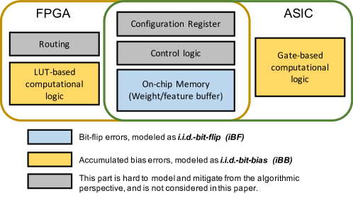
The possible errors in CMOS-based platforms are illustrated in Fig. 1. Soft errors that happen in the memory elements or the logic elements could lead to transient faulty outputs in ASICs. Compared with logic elements (e.g., combinational logic gates, flip-flops), memory elements are more susceptible to soft errors (Slayman, 2011). An unprotected SRAM cell usually has a larger bit soft error rate (SER) than flip-flops. Since the occurring probability of hard errors is much smaller than that of the soft errors, we focus on the analysis of soft errors, despite that hard errors lead to permanent failures.
The soft errors in the weight buffer could be modeled as i.i.d weight random bit-flips. Given the original value as , the distribution of a faulty value under the random bit-flip (BF) model could be written as
| (6) | ||||
where denotes whether a bit-flip occurs at bit position , is the XOR operator.
By assuming that error occurs at each bit with an i.i.d bit SER of , we know that each -bit weight has an i.i.d probability to encounter error, and , as . It is worth noting that throughout the analysis, we assume that the SERs of all components , hence the error rate at each level is approximated as the sum of the error rates of the independent sub-components. As each weight encounters error independently, a weight tensor is distributed as i.i.d random bit-flip (iBF): , where is the golden weights. Reagen et al. (2018) showed that the iBF model could capture the bit error behavior exhibited by real SRAM hardware.
The soft errors in the feature buffer are modeled similarly as i.i.d random bit-flips, with a fault probability of approximately for -bit feature values. The distribution of the output feature map (OFM) values could be written as , where is the golden results.
Actually, FPGA-based implementations are usually more vulnerable to soft errors than their ASIC counterparts (Asadi and Tahoori, 2007). Since the majority space of an FPGA chip is filled with memory cells, the overall SER rate is much higher. Moreover, the soft errors occurring in logic configuration bits would lead to persistent faulty computation, rather than transient faults as in ASIC logic. Persistent errors can not be mitigated by simple retry methods and would lead to statistically significant performance degradation. Moreover, since the persistent errors would be accumulated if no correction is made, the equivalent error rate would keep increasing as time goes on. We abstract this effect with a monotonic increasing function , where the subscript denotes “persistent”, and denotes the time. For example, if the FPGA weight buffer or LUTs are reloaded for every period in the radioactive environment (Bolchini et al., 2007; Carmichael et al., 2000), a multiplier of would be the worst bounding case. Note that the exact choice of is not important in our experiments, since our work mainly aims at comparing different neural architectures using certain fault insertion pattern and ratio, and the temporal effect modeled by does not influence the architectural preference.
Let us recap how one convolution is mapped onto the FPGA-based accelerator, to see what the configuration bit errors could cause on the OFM values. If the dimension of the convolution kernel is (channel, kernel height, kernel width, respectively), there are additions needed for the computation of a feature value. We assume that the add operations are spatially expanded onto adder trees constructed by LUTs, i.e., no temporal reusing of adders is used for computing one feature value. That is to say, the add operations are mapped onto different hardware adders333See more discussion in Sec. 6.4., and encounter errors independently. The per-feature error rate could be approximated by the adder-wise SER times , where . Now, let’s dive into the adder-level computation, in a 1-bit adder with scale , the bit-flip in one LUTs bit would add a bias to the output value, if the input bit signals match the address of this LUTs bit. If each LUT cell has an i.i.d SER of , in a -bit adder, denoting the fraction length of the operands and result as , the distribution of the faulty output with the random bit-bias (BB) faults could be written as
| (7) | ||||
As for the result of the adder tree constructed by multiple LUT-based adders, since the probability that multiple bit-bias errors co-occur is orders of magnitude smaller, we ignore the accumulation of the biases that are smaller than the OFM quantization resolution . Consequently, the OFM feature values before the activation function follow the i.i.d Random Bit-Bias distribution , where and are the bit-width and fraction length of the OFM values, respectively.
We can make an intuitive comparison between the equivalent feature error rates induced by LUTs soft errors and feature buffer soft errors. As the majority of FPGAs is SRAM-based, considering the bit SER of LUTs cell and BRAM cell to be close, we can see that the feature error rate induced by LUTs errors is amplified by . As we have discussed, , the performance degradation induced by LUTs errors could be significantly larger than that induced by feature buffer errors.
3.3. Analysis of PIM-based Platforms: RRAM as an example
In an RRAM-based computing system, compared with the accompanying CMOS circuits, the RRAM crossbar is much more vulnerable to various non-ideal factors. In multi-bit RRAM cells, studies have showed that the distribution of the resistance due to programming variance is either Gaussian or Log-Normal (Le et al., 2018). As each weight is programmed as the conductance of the memristor cell, the weight could be seen as being distributed as Reciprocal-Normal or Log-Normal. Besides the soft errors, common hard errors such as SAFs, caused by fabrication defects or limited endurance, could result in severe performance degradation (Xia et al., 2018). SAFs occur frequently in nowadays RRAM crossbar: As reported by (Chen et al., 2015), the overall SAF ratio could be larger than 10% ( for SAF1 and for SAF0) in a fabricated RRAM device. The statistical model of SAFs in single-bit and multi-bit RRAM devices would be formalized in Sec. 3.5.
As the RRAM crossbars also serve as the computation units, some non-ideal factors (e.g., IR-drop, wire resistance) could be abstracted as feature faults. They are not considered in this work since the modeling of these effects highly depends on the implementation (e.g., crossbar dimension, mapping strategy) and hardware-in-the-loop testing (He et al., 2019).
3.4. Feature Fault Model
As analyzed in Sec. 3.2, the soft errors in LUTs are relatively the more pernicious source of feature faults, as 1) SER is usually much higher than hard error rate: , 2) these errors are persistent if no correction is made, 3) the per-feature equivalent error rate is amplified as multiple adders are involved. Therefore, we use the iBB fault model in our exploration of mitigating feature faults.
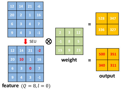
We have , where , and the probability of error occurring at every position in the OFM is , where is defined as the per-MAC error rate. Denoting the dimension of the OFM as (channel, height, and width, respectively) and the dimension of each convolution kernel as , the computation of a convolution layer under this fault model could be written as
| (8) | ||||
where is the mask indicating whether an error occurs at each feature map position, represents the bit position of the bias, represents the bias sign. Note that this formulation is not equivalent to the random bit-bias formalization in Eq. 7, and is adopted for efficient simulation. These two formulations are close when the odds that two errors take effect simultaneously is small (). This fault model is referred to as the MAC-i.i.d Bit-Bias model (abbreviated as MiBB). An example of injecting this type of feature faults is illustrated in Fig. 2.
Intuitively, convolution computation that needs fewer MACs might be more immune to the faults, as the equivalent error rate at each OFM location is lower.
3.5. Weight Fault Model
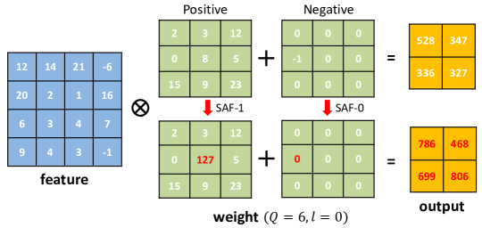
As RRAM-based accelerators suffer from a much higher weight error rate than the CMOS-based ones. The Stuck-at-Faults in RRAM crossbars are mainly considered for the setup of the weight fault model. We assume the underlying platform is RRAM with multi-bit cells, and adopt the commonly-used mapping scheme, in which separate crossbars are used for storing positive and negative weights (Chi et al., 2016). That is to say, when an SAF0 fault causes a cell to be stuck at HRS, the corresponding logical weight would be stuck at 0. When an SAF1 fault causes a cell to be stuck at LRS, the weight would be stuck at if it’s negative, or otherwise.
The computation of a convolution layer under the SAF weight fault model could be written as
| (9) | ||||
where refers to the representation bound in Eq. 3, is the mask indicating whether fault occurs at each weight position, is the mask representing the SAF types (SAF0 or SAF1) at faulty weight positions, is the mask representing the faulty target values ( or ). Every single weight has an i.i.d probability of to be stuck at , and to be stuck at the positive or negative bounds of the representation range, for positive and negative weights, respectively. An example of injecting this type of weight faults is illustrated in Fig. 3.
Note that the weight fault model, referred to as arbitrary-distributed Stuck-at-Fault model (adSAF), is much harder to defend against than SAF faults with a specific known defect map. A neural network model that behaves well under the adSAF model is expected to achieve high reliability across different specific SAF defect maps.
The above adSAF fault model assumes the underlying hardware is multi-bit RRAM devices, adSAFs in single-bit RRAM devices are also of interest. In single-bit RRAM devices, multiple bits of one weight value are mapped onto different crossbars, of which the results would be shifted and added together (Zhu et al., 2019). In this case, an SAF fault that occurs in a cell would cause the corresponding bit of the corresponding weight to be stuck at or . The effects of adSAF faults on a weight value in single-bit RRAM devices can be formulated as
| (10) | ||||
where the binary representation of indicates whether fault occurs at each bit position, the binary representation of represents the target faulty values ( or ) at each bit position if fault occurs. We will demonstrate that the architecture discovered under the multi-bits adSAF fault model can also defend against single-bit adSAF faults and iBF weight faults caused by errors in the weight buffers of CMOS-based accelerators.
4. Fault-Tolerant NAS
In this section, we present the FTT-NAS framework. We first give out the problem formalization and framework overview in Sec. 4.1. Then, the search space, sampling and assembling process are described in Sec. 4.2 and Sec. 4.3, respectively. Finally, the search process is elaborated in Sec. 4.4.
4.1. Framework Overview
Denoting the fault distribution characterized by the fault models as , the neural network search for fault tolerance can be formalized as
| (11) | ||||
where is the architecture search space, and denote the training and validation data split, respectively. and denote the reward and loss criterion, respectively. The major difference of Eq. 11 to the vanilla NAS problem Eq. 5 lies in the introduction of the fault model .
As the cost of finding the best weights for each architecture is almost unbearable, we use the shared-weights based evaluator, in which shared weights are directly used to evaluate sampled architectures. The resulting method, FTT-NAS, is the method to solve this NAS problem approximately. And FT-NAS can be viewed as a degraded special case for FTT-NAS, in which no fault is injected in the inner optimization of finding .
The overall neural architecture search framework is illustrated in Fig. 4 (b). There are multiple components in the framework: A controller that samples different architecture rollouts from the search space; A candidate network is assembled by taking out the corresponding subset of weights from the super-net. A shared weights based evaluator evaluates the performance of different rollouts on the CIFAR10 dataset, using fault-tolerant objectives.
4.2. Search Space
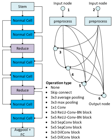
The design of the search space is as follows: We use a cell-based macro architecture, similar to the one used in (Pham et al., 2018; Liu et al., 2019a). There are two types of cells: normal cell, and reduction cell with stride 2. All normal cells share the same connection topology, while all reduction cells share another connection topology. The layout and connections between cells are illustrated in Fig. 5.
In every cell, there are nodes, node 1 and node 2 are treated as the cell’s inputs, which are the outputs of the two previous cells. For each of the other nodes, two in-coming connections will be selected and element-wise added. For each connection, the 11 possible operations are: none; skip connect; 3x3 average (avg.) pool; 3x3 max pool; 1x1 Conv; 3x3 ReLU-Conv-BN block; 5x5 ReLU-Conv-BN block; 3x3 SepConv block; 5x5 SepConv block; 3x3 DilConv block; 5x5 DilConv block.
The complexity of the search space can be estimated. For each cell type, there are possible choices. As there are two independent cell types, there are possible architecture in the search space, which is roughly with in our experiments.
4.3. Sampling and Assembling Architectures
In our experiments, the controller is an RNN, and the performance evaluation is based on a super network with shared weights, as used by (Pham et al., 2018).
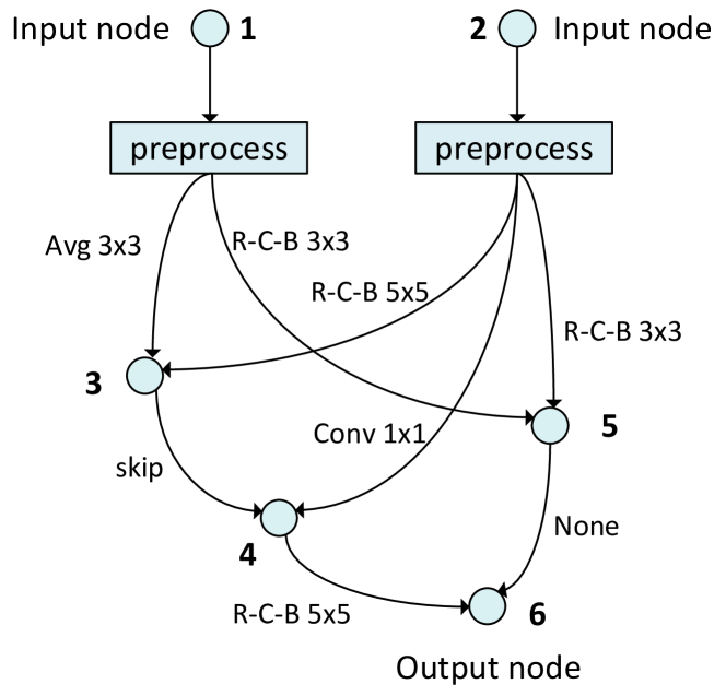
An example of the sampled cell architecture is illustrated in Fig. 6. Specifically, to sample a cell architecture, the controller RNN samples blocks of decisions, one for each node . In the decision block for node , input nodes are sampled from , to be connected with node . Then operations are sampled from the basic operation primitives, one for each of the connections. Note that the two sampled input nodes can be the same node , which will result in two independent connections from node to node .
During the search process, the architecture assembling process using the shared-weights super network is straightforward (Pham et al., 2018): Just take out the weights from the super network corresponding to the connections and operation types of the sampled architecture.
4.4. Searching for Fault-Tolerant Architecture
The FTT-NAS algorithm is illustrated in Alg. 1. To search for a fault-tolerant architecture, we use a weighted sum of the clean accuracy and the accuracy with fault injection as the reward to instruct the training of the controller:
| (12) |
where is calculated by injecting faults following the fault distribution described in Sec. 3. For the optimization of the controller, we employ the Adam optimizer (Kingma and Ba, 2015) to optimize the REINFORCE (Williams, 1992) objective, together with an entropy encouraging regularization.
In every epoch of the search process, we alternatively train the shared weights and the controller on separate data splits and , respectively. For the training of the shared weights, we carried out experiments under two different settings: without/with FTT. When training with FTT, a weighted sum of the clean cross entropy loss and the cross entropy loss with fault injection is used to train the shared weights. The FTT loss can be written as
| (13) |
As shown in line 7-12 in Alg. 1, in each step of training the shared weights, we sample architecture using the current controller, then backpropagate using the FTT loss to update the parameters of the candidate network. Training without FTT (in FT-NAS) is a special case with .
As shown in line 15-20 in Alg. 1, in each step of training the controller, we sample architecture from the controller, assemble this architecture using the shared weights, and then get the reward on one data batch in . Finally, the reward is used to update the controller by applying the REINFORCE technique (Williams, 1992), with the reward baseline denoted as .
5. Experiments
In this section, we demonstrate the effectiveness of the FTT-NAS framework and analyze the discovered architectures under different fault models. First, we introduce the experiment setup in Sec. 5.1. Then, the effectiveness under the feature and weight fault models are shown in Sec. 5.2 and Sec. 5.3, respectively. The effectiveness of the learned controller is illustrated in Sec. 5.4. Finally, the analyses and illustrative experiments are presented in Sec. 5.5.
5.1. Setup
Our experiments are carried out on the CIFAR-10 (Krizhevsky, 2009) dataset. CIFAR-10 is one of the most commonly used computer vision datasets and contains 60000 RGB images. Three manually designed architectures VGG-16, ResNet-18, and MobileNet-V2 are chosen as the baselines. 8-bit dynamic fixed-point quantization is used throughout the search and training process, and the fraction length is found following the minimal-overflow principle.
In the neural architecture search process, we split the training dataset into two subsets. 80% of the training data is used to train the shared weights, and the remaining 20% is used to train the controller. The super network is an 8-cell network, with all the possible connections and operations. The channel number of the first cell is set to 20 during the search process, and the channel number increases by 2 upon every reduction cell. The controller network is an RNN with one hidden layer of size 100. The learning rate for training the controller is 1e-3. The reward baseline is updated using a moving average with momentum 0.99. To encourage exploration, we add an entropy encouraging regularization to the controller’s REINFORCE objective, with a coefficient of . For training the shared weights, we use an SGD optimizer with momentum 0.9 and weight decay 1e-4, the learning rate is scheduled by a cosine annealing scheduler (Loshchilov and Hutter, 2017), started from . Each architecture search process is run for 100 epochs. Note that all these are typical settings that are similar to (Pham et al., 2018).
To conduct the final training of the architectures (Fig.4 (c)), we run fault-tolerant training for 100 epochs. The learning rate is set to initially and decayed by at epoch 40 and 80. We have experimented with a fault-tolerant training choice: whether to mask out the error positions in feature/weights during the backpropagation process. If the error positions are masked out, then no gradient would be backpropagated through the erroneous feature positions, and no gradient would be calculated w.r.t. the erroneous weight positions. We find that this choice does not affect the fault-tolerant training result, thus we do not use the masking operation in our final experiments.
We build the neural architecture search framework and fault injection framework upon the PyTorch framework, and all the codes are available at https://github.com/walkerning/aw_nas.
5.2. Defend Against MiBB Feature Faults
| Arch | Training† | Clean accuracy | Accuracy (%) with feature faults | #FLOPs | #Params | ||||
|---|---|---|---|---|---|---|---|---|---|
| 3e-6 | 1e-5 | 3e-5 | 1e-4 | 3e-4 | |||||
| ResNet-18 | clean | 94.7 | 89.1 | 63.4 | 11.5 | 10.0 | 10.0 | 1110M | 11.16M |
| VGG-16 | clean | 93.1 | 78.2 | 21.4 | 10.0 | 10.0 | 10.0 | 626M | 14.65M |
| MobileNet-V2 | clean | 92.3 | 10.0 | 10.0 | 10.0 | 10.0 | 10.0 | 182M | 2.30M |
| F-FT-Net | clean | 91.0 | 71.3 | 22.8 | 10.0 | 10.0 | 10.0 | 234M | 0.61M |
| ResNet-18 | =1e-4 | 79.2 | 79.1 | 79.6 | 78.9 | 60.6 | 11.3 | 1110M | 11.16M |
| VGG-16 | =3e-5 | 83.5 | 82.4 | 77.9 | 50.7 | 11.1 | 10.0 | 626M | 14.65M |
| MobileNet-V2 | =3e-4 | 71.2 | 70.3 | 69.0 | 68.7 | 68.1 | 47.8 | 182M | 2.30M |
| F-FTT-Net | =3e-4 | 88.6 | 88.7 | 88.5 | 88.0 | 86.2 | 51.0 | 245M | 0.65M |
: As also noted in the main text, for all the FTT trained models, we successively try per-MAC fault injection probability in {3e-4, 1e-4, 3e-5}, and use the largest injection probability with which the model could achieve a clean accuracy above 50%.
As described in Sec. 4, we conduct neural architecture searching without/with fault-tolerant training (i.e., FT-NAS and FTT-NAS, correspondingly). The per-MAC injection probability used in the search process is 1e-4. The reward coefficients in Eq. 12 is set to . In FTT-NAS, the loss coefficient in Eq. 13 is also set to . As the baselines for FT-NAS and FTT-NAS, we train ResNet-18, VGG-16, MobileNet-V2 with both normal training and FTT. For each model trained with FTT, we successively try per-MAC fault injection probability in {3e-4, 1e-4, 3e-5}, and use the largest injection probability with which the model could achieve a clean accuracy above 50%. Consequently, the ResNet-18 and VGG-16 are trained with a per-MAC fault injection probability of 1e-4 and 3e-5, respectively.
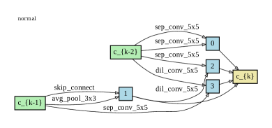
The discovered cell architectures are shown in Fig. 7, and the evaluation results are shown in Table 4. The discovered architecture F-FTT-Net outperforms the baselines significantly at various fault ratios. In the meantime, compared with the most efficient baseline MobileNet-V2, the FLOPs number of F-FTT-Net is comparable, and the parameter number is only 28.3% (0.65M versus 2.30M). If we require that the accuracy should be kept above , MobileNet-V2 could function with a per-MAC error rate of 3e-6, and F-FTT-Net could function with a per-MAC error rate larger than 1e-4. That is to say, while meeting the same accuracy requirements, F-FTT-Net could function in an environment with a much higher SER.
We can see that FTT-NAS is much more effective than its degraded variant, FT-NAS. We conclude that, generally, NAS should be used in conjunction with FTT, as suggested by Eq. 11. Another interesting fact is that, under the MiBB fault model, the relative rankings of the resilience capabilities of different architectures change after FTT: After FTT, MobileNet-V2 suffers from the smallest accuracy degradation among 3 baselines, whereas it is the most vulnerable one without FTT.
5.3. Defend Against adSAF Weight Faults
We conduct FT-NAS and FTT-NAS under the adSAF model. The overall SAF ratio is set to 8%, in which the proportion of SAF0 and SAF1 is 83.7% and 16.3%, respectively (SAF0 ratio =6.7%, SAF1 ratio =1.3%). The reward coefficient is set to . The loss coefficient in FTT-NAS is set to . After the fault-tolerant training of the discovered architecture, we test the model accuracy with various SAF ratios (from 4% to 12%), while the relative ratio remains unchanged according to the numbers reported by Chen et al. (2015).
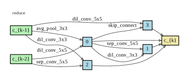
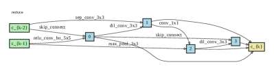
The discovered cell architectures are shown in Fig. 8. As shown in Table 5, the discovered W-FTT-Net outperforms the baselines significantly at various test SAF ratios, with comparable FLOPs and less parameter number. We then apply channel augmentation to the discovered architecture to explore the performance of the model at different scales. We can see that models with larger capacity have better reliability under the adSAF weight fault model, e.g., (W-FTT-Net-40) VS. (W-FTT-Net-20) with 10% adSAF faults.
| Arch | Training | Clean accuracy | Accuracy (%) with weight faults | #FLOPs | #Params | ||||
|---|---|---|---|---|---|---|---|---|---|
| 0.04 | 0.06 | 0.08 | 0.10 | 0.12 | |||||
| ResNet-18 | clean | 94.7 | 64.8 | 34.9 | 17.8 | 12.4 | 11.0 | 1110M | 11.16M |
| VGG-16 | clean | 93.1 | 45.7 | 21.7 | 14.3 | 12.6 | 10.6 | 626M | 14.65M |
| MobileNet-V2 | clean | 92.3 | 26.2 | 14.3 | 11.7 | 10.3 | 10.5 | 182M | 2.30M |
| W-FT-Net-20 | clean | 91.7 | 54.2 | 30.7 | 19.6 | 15.5 | 11.9 | 1020M | 3.05M |
| ResNet-18 | =0.08 | 92.0 | 86.4 | 77.9 | 60.8 | 41.6 | 25.6 | 1110M | 11.16M |
| VGG-16 | =0.08 | 91.1 | 82.6 | 73.3 | 58.5 | 41.7 | 28.1 | 626M | 14.65M |
| MobileNet-V2 | =0.08 | 86.3 | 76.6 | 55.9 | 35.7 | 18.7 | 15.1 | 182M | 2.30M |
| W-FTT-Net-20† | =0.08 | 90.8 | 86.2 | 79.5 | 69.6 | 53.5 | 38.4 | 919M | 2.71M |
| W-FTT-Net-40 | =0.08 | 92.1 | 88.8 | 85.5 | 79.3 | 69.2 | 54.2 | 3655M | 10.78M |
: The “-” suffix means that the base of the channel number is .
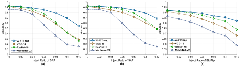
In order to investigate whether the model FTT-trained under the adSAF fault model can tolerate other types of weight faults, we evaluate the reliability of W-FTT-Net under 1bit-adSAF model and the iBF model. As shown in Fig. 9 (b)(c), under the 1bit-adSAF and iBF weight fault model, W-FTT-Net outperforms all the baselines consistently at different noise levels.
5.4. The Effectiveness of The Learned Controller
To demonstrate the effectiveness of the learned controller, we compare the performance of the architectures sampled by the controller, with the performance of the architectures random sampled from the search space. For both the MiBB feature fault model and the adSAF weight fault model, we random sample architectures from the search space, and train them with FTT for 100 epochs. A per-MAC fault injection probability of 3e-4 is used for feature faults, and an SAF ratio of (=6.7%, =1.3%) is used for weight faults.
As shown in Table 6 and Table 7, the performance of different architectures in the search space varies a lot, and the architectures sampled by the learned controllers, F-FTT-Net and W-FTT-Net, outperform all the random sampled architectures. Note that, as we use different preprocess operations for feature faults and weight faults (ReLU-Conv-BN 3x3 and SepConv 3x3, respectively), there exist differences in FLOPs and parameter number even with the same cell architectures.
| Model | clean acc | =3e-4 | #FLOPs | #Params |
|---|---|---|---|---|
| sample1 | 60.2 | 19.5 | 281M | 0.81M |
| sample2 | 79.7 | 29.7 | 206M | 0.58M |
| sample3 | 25.0 | 32.2 | 340M | 1.09M |
| sample4 | 32.9 | 25.8 | 387M | 1.23M |
| sample5 | 17.4 | 10.8 | 253M | 0.77M |
| F-FTT-Net | 88.6 | 51.0 | 245M | 0.65M |
| Model | clean acc | =8% | #FLOPs | #Params |
|---|---|---|---|---|
| sample1 | 90.7 | 63.6 | 705M | 1.89M |
| sample2 | 84.7 | 36.7 | 591M | 1.54M |
| sample3 | 90.3 | 60.3 | 799M | 2.33M |
| sample4 | 90.5 | 64.0 | 874M | 2.55M |
| sample5 | 85.2 | 45.6 | 665M | 1.83M |
| W-FTT-Net | 90.7 | 68.5 | 919M | 2.71M |
5.5. Inspection of the Discovered Architectures
Feature faults: From the discovered cell architectures shown in Fig. 7, we can observe that the controller obviously prefers SepConv and DilConv blocks over Relu-Conv-BN blocks. This observation is consistent with our anticipation. As under the MiBB feature fault model, operations with smaller FLOPs will result in a lower equivalent fault rate in the OFM.
Under the MiBB feature fault model, there is a tradeoff between the capacity of the model and the feature error rate. As the number of channels increases, the operations become more expressive, but the equivalent error rates in the OFMs also get higher. Thus there exists a tradeoff point of for the number of channels. Intuitively, depends on the per-MAC error rate , the larger the is, the smaller the is.
Besides the choices of primitives, the connection pattern and combination of different primitives also play a role in making the architecture fault-tolerant. To verify this, first, we conduct a simple experiment to confirm the preference of primitives: For each of the 4 different primitives (SepConv 3x3, SepConv 5x5, DilConv 3x3, DilConv 5x5), we stack 5 layers of the primitives, get the performance of the stacked NN after FTT training it with =3e-4. The stacked NNs
achieve the accuracy of 60.0%, 65.1%, 50.0% and 56.3% with 1e-4, respectively. The stacked NN of SepConv 5x5 blocks achieves the best performance, which is of no surprise since the most frequent block in F-FTT-Net is SepConv5x5. Then, we construct six architectures by random sampling five architectures with only SepConv5x5 connections and replacing all the primitives in F-FTT-Net with SepConv 5x5 blocks. The best result achieved by these six architecture is 77.5% with 1e-4 (versus 86.2% achieved by F-FTT-Net). These illustrative experiments indicate that the connection pattern and combination of different primitives all play a role in the fault resilience capability of a neural network architecture.
Weight faults: Under the adSAF fault model, the controller prefers ReLU-Conv-BN blocks over SepConv and DilConv blocks. This preference is not so easy to anticipate. We hypothesise that the weight distribution of different primitives might lead to different behaviors when encountering SAF faults. For example, if the quantization range of a weight value is larger, the value deviation caused by an SAF1 fault would be larger, and we know that a large increase in the magnitude of weights would damage the performance severely (Hacene et al., 2019). We conduct a simple experiment to verify this hypothesis: We stack several blocks to construct a network, and in each block, one of the three operations (a SepConv3x3 block, a ReLU-Conv-BN 3x3 block, and a ReLU-Conv-BN 1x1 block) is randomly picked in every training step. The SepConv 3x3 block is constructed with a DepthwiseConv 3x3 and two Conv 1x1, and the ReLU-Conv-BN 3x3 and ReLU-Conv-BN 1x1 contain a Conv 3x3 and a Conv 1x1, respectively. After training, the weight magnitude ranges of Conv 3x3, Conv 1x1, and DepthwiseConv 3x3 are 0.0360.043, 0.1120.121, 0.1400.094, respectively. Since the magnitude of the weights in 3x3 convolutions is smaller than that of the 1x1 convolutions and the depthwise convolutions, SAF weight faults would cause larger weight deviations in a SepConv or DilConv block than in a ReLU-Conv-BN 3x3 block.
6. Discussion
6.1. Orthogonality
Most of the previous methods are exploiting the inherent fault resilience capability of existing NN architectures to tolerate different types of hardware faults. In contrast, our methods improve the inherent fault resilience capability of NN models, thus effectively increase the algorithmic fault resilience “budget” to be utilized by hardware-specific methods. Our methods are orthogonal to existing fault-tolerance methods, and can be easily integrated with them, e.g., helping hardware-based methods to reduce the overhead largely.
6.2. Data representation
In our work, an 8-bit dynamic fixed-point representation is used for the weights and features. As pointed out in Sec. 5.5, the dynamic range has impacts on the resilience characteristics against weight faults. The data format itself obviously decides or affects the data range. Yan et al. (2020) found out that the errors in exponent bits of the 32bit floating-point weights have large impacts on the performance. Li et al. (2017) investigated the resilience characteristics of several floating-point and non-dynamic fixed-point representations.
6.3. Other search strategies (controllers)
A NAS system mainly consists of three components that work together: The search space that defines the architectural decisions to make; The evaluator that assesses the performance of an architecture; The search strategy (controller) that explores the search space using the rewards provided by the evaluator. Apart from few exceptions such as the differentiable NAS methods (Liu et al., 2019a), the NAS system could be built in a modularized and decoupled way, in which the controller and the evaluator can be designed independently. Our major modifications to the NAS framework lie in that 1) We analyze different categories of faults existing in various devices, and conduct fault insertion with the formulated fault model when evaluating the reward. 2) The fault-tolerant training techniques should be incorporated when training the supernet weights, to reduce the gap between the search and final training stages, since it is a common technique for training a fault-tolerant NN model. Note that these two amendments are all on the evaluator component. Despite that we choose to use the popular reinforcement learning-based controller, other controllers such as evolutionary-based (Real et al., 2019) and predictor-based ones (Ning et al., 2020) could be incorporated into the FTT-NAS framework easily. The application of other controllers is outside the scope of this work’s interests.
6.4. Fault model
Limitation of application-level fault model: There are faults that are hard or unlikely to model and mitigate by our methods, e.g., timing errors, routing/DSP errors in FPGA, etc. A hardware-in-the-loop framework could be established for a thorough evaluation of the system-level fault hazards. Anyway, since the correspondence between these faults and the application-level elements are subtle, it’s more suitable to mitigate these faults in the lower abstraction layer.
FPGA platform:
In the MiBB feature fault model, we assume that the add operations are spatially expanded onto independent hardware adders, which applies to the template-based designs (Venieris and
Bouganis, 2019). For ISA (Instruction Set Architecture) based accelerators (Qiu et al., 2016), the NN computations are orchestrated using instructions, time-multiplexed onto hardware units. In this case, the accumulation of the faults follows a different model and might show different preferences among architectures. Anyway, the FTT-NAS framework is general and could be used with different fault models. We leave the exploration and experiments of other fault models for future work.
RRAM platform:
As for the RRAM platform, this paper mainly focuses on discovering fault-tolerant neural architecture to mitigate SAFs, which have significant impacts on computing accuracy. In addition to SAFs, the variation is another typical RRAM non-ideal factor that may lead to inaccurate computation. There exist various circuit-level optimizations that can mitigate the computation error caused by the RRAM variation.
Firstly, with the development of the RRAM device technology, a large on/off ratio of RRAM devices (i.e., the resistance ratio of the high resistance state and the low resistance state) can be obtained (e.g., (Woo et al., 2020)). And a large on/off ratio makes the bit line current difference among different computation results obvious and thus improves the fault tolerance capability against variation. Secondly, in existing RRAM-based accelerators, the number of activated RRAM rows at one time is limited. For example, only four rows are activated in each cycle, which provides a sufficient signal margin against process variation (Xue
et al., 2021). In contrast, compared with the process variation, it is more costly to mitigate SAFs by circuit-level optimization (e.g., existing work utilizes costly redundant hardware to tolerate SAFs (Huangfu et al., 2017)). Thus, we aim at tolerating the SAFs from the algorithmic perspective. Anyway, simulating the variation is a meaningful extension of the general FTT-NAS framework for the RRAM platform, and we leave it for future work.
Combining multiple fault models: We experiment with a fault model at a time, and do not combine different fault models. And our experimental results show that the architectural preferences of the adSAF and iBB feature fault models are distinct (See discussions in Sec. 5.5). Fortunately, the two types of faults that we experiment with would not co-exist for the same part of an NN model: IBB feature faults (caused by FPGA LUTs errors) and the adSAF weight faults (in the RRAM crossbar). Nevertheless, there indeed exist scenarios that some weights and feature errors could happen simultaneously on one platform. For example, iBF in the feature buffer and SAF in the crossbar can occur simultaneously in an RRAM-based accelerator. However, on the same platform in the same environment, the influences of different types of errors would usually be vastly different. For example, compared with the accuracy degradation caused by the SAF errors in the RRAM cell, the influences of iBF errors in the feature buffer could usually be ignored on the same device.
As a future direction, it might be interesting to combine these fault models to search for a neural architecture to be partitioned and deployed onto a heterogeneous hardware system. In that case, the fault patterns, along with the computation and memory access patterns of multiple platforms should be considered jointly.
7. Conclusion
In this paper, we analyze the possible faults in various types of NN accelerators and formalize the statistical fault models from the algorithmic perspective. After the analysis, the MAC-i.i.d Bit-Bias (MiBB) model and the arbitrary-distributed Stuck-at-Fault (adSAF) model are adopted in the neural architecture search for tolerating feature faults and weight faults, respectively. To search for the fault-tolerant neural network architectures, we propose the multi-objective Fault-Tolerant NAS (FT-NAS) and Fault-Tolerant Training NAS (FTT-NAS) method. In FTT-NAS, the NAS technique is employed in conjunction with the Fault-Tolerant Training (FTT). The fault resilience capabilities of the discovered architectures, F-FTT-Net and W-FTT-Net, outperform multiple manually designed architecture baselines, with comparable or fewer FLOPs and parameters. And W-FTT-Net trained under the 8bit-adSAF model can defend against other types of weight faults. Generally, compared with FT-NAS, FTT-NAS is more effective and should be used. In addition, through the inspection of the discovered architectures, we find that since operation primitives differ in their MACs, expressiveness, weight distributions, they exhibit different resilience capabilities under different fault models. The connection pattern is also shown to have influences on the fault resilience capability of NN models.
Acknowledgements.
This work was supported by National Natural Science Foundation of China (No. U19B2019, 61832007, 61621091), National Key R&D Program of China (No. 2017YFA02077600); Beijing National Research Center for Information Science and Technology (BNRist); Beijing Innovation Center for Future Chips; the project of Tsinghua University and Toyota Joint Research Center for AI Technology of Automated Vehicle (TT2020-01); Beijing Academy of Artificial Intelligence.References
- (1)
- Arechiga and Michaels (2018) Austin P. Arechiga and Alan J. Michaels. 2018. The Robustness of Modern Deep Learning Architectures against Single Event Upset Errors. 2018 IEEE High Performance extreme Computing Conference (HPEC), 1–6.
- Asadi and Tahoori (2007) Hossein Asadi and Mehdi B Tahoori. 2007. Analytical Techniques for Soft Error Rate Modeling and Mitigation of FPGA-Based Designs. IEEE Transactions on Very Large Scale Integration Systems (TVLSI) 15, 12 (Dec 2007), 1320–1331.
- Baker et al. (2017) Bowen Baker, Otkrist Gupta, R. Raskar, and N. Naik. 2017. Accelerating neural architecture search using performance prediction. arXiv preprint arXiv:1705.10823 (2017).
- Bolchini et al. (2007) Cristiana Bolchini, Antonio Miele, and Marco D Santambrogio. 2007. TMR and Partial Dynamic Reconfiguration to mitigate SEU faults in FPGAs. IEEE International Symposium on Defect and Fault Tolerance in VLSI Systems (DFT) (2007), 87–95.
- Borkar (2005) Shekhar Borkar. 2005. Designing reliable systems from unreliable components: the challenges of transistor variability and degradation. IEEE Micro 25, 6 (2005), 10–16.
- Carmichael et al. (2000) Carl Carmichael, Michael Caffrey, and Anthony Salazar. 2000. Correcting single-event upsets through Virtex partial configuration. Xilinx Application Notes 216 (2000), v1.
- Chen et al. (2015) Ching-Yi Chen, Hsiu-Chuan Shih, Cheng-Wen Wu, C. Lin, Pi-Feng Chiu, S. Sheu, and F. Chen. 2015. RRAM Defect Modeling and Failure Analysis Based on March Test and a Novel Squeeze-Search Scheme. IEEE Trans. Comput. 64, 1 (Jan 2015), 180–190.
- Chen et al. (2017) Lerong Chen, Jiawen Li, Yiran Chen, Qiuping Deng, Jiyuan Shen, X. Liang, and L. Jiang. 2017. Accelerator-friendly neural-network training: Learning variations and defects in RRAM crossbar. In IEEE/ACM Proceedings Design, Automation and Test in Eurpoe (DATE). 19–24.
- Chen et al. (2014) Tianshi Chen, Zidong Du, Ninghui Sun, J. Wang, Chengyong Wu, Yunji Chen, and Olivier Temam. 2014. DianNao: a small-footprint high-throughput accelerator for ubiquitous machine-learning. In ACM International Conference on Architectural Support for Programming Languages and Operating Systems (ASPLOS).
- Chi et al. (2016) Ping Chi, Shuangchen Li, C. Xu, Tao Zhang, J. Zhao, Yongpan Liu, Y. Wang, and Yuan Xie. 2016. PRIME: A Novel Processing-in-memory Architecture for Neural Network Computation in ReRAM-based Main Memory. In IEEE/ACM International Symposium on Computer Architecture (ISCA). IEEE Press, 27–39.
- Guo et al. (2019) Kaiyuan Guo, Shulin Zeng, Jincheng Yu, Yu Wang, and Huazhong Yang. 2019. A Survey of FPGA-based Neural Network Inference Accelerators. ACM Transactions on Reconfigurable Technology and Systems (TRETS) 12, 1, Article 2 (March 2019), 26 pages.
- Hacene et al. (2019) Ghouthi Boukli Hacene, François Leduc-Primeau, Amal Ben Soussia, Vincent Gripon, and F. Gagnon. 2019. Training Modern Deep Neural Networks for Memory-Fault Robustness. IEEE International Symposium on Circuits and Systems (ISCAS) (2019), 1–5.
- Haghi and Draper (2009) Mahta Haghi and Jeff Draper. 2009. The 90 nm Double-DICE storage element to reduce Single-Event upsets. In IEEE International Midwest Symposium on Circuits and Systems (MWSCAS). IEEE, 463–466.
- He et al. (2016) Kaiming He, Xiangyu Zhang, Shaoqing Ren, and Jian Sun. 2016. Deep Residual Learning for Image Recognition. IEEE Conference on Computer Vision and Pattern Recognition (CVPR) (2016), 770–778.
- He et al. (2019) Zhezhi He, Jie Lin, Rickard Ewetz, J. Yuan, and Deliang Fan. 2019. Noise Injection Adaption: End-to-End ReRAM Crossbar Non-ideal Effect Adaption for Neural Network Mapping. In ACM/IEEE Design Automation Conference (DAC). ACM.
- Henkel et al. (2013) Jörg Henkel, Lars Bauer, Nikil Dutt, Puneet Gupta, Sani Nassif, Muhammad Shafique, Mehdi Tahoori, and Norbert Wehn. 2013. Reliable on-chip systems in the nano-era: Lessons learnt and future trends. In ACM/IEEE Design Automation Conference (DAC). IEEE, 1–10.
- Hu et al. (2013) Miao Hu, Hai Li, Yiran Chen, Q. Wu, and G. Rose. 2013. BSB training scheme implementation on memristor-based circuit. In IEEE Symposium on Computational Intelligence for Security and Defense Applications (CISDA). IEEE, 80–87.
- Huangfu et al. (2017) Wenqin Huangfu, Lixue Xia, Ming Cheng, Xiling Yin, Tianqi Tang, Boxun Li, Krishnendu Chakrabarty, Yuan Xie, Yu Wang, and Huazhong Yang. 2017. Computation-oriented fault-tolerance schemes for RRAM computing systems. In IEEE/ACM Asia and South Pacific Design Automation Conference (ASPDAC). IEEE, 794–799.
- Hubara et al. (2017) Itay Hubara, Matthieu Courbariaux, Daniel Soudry, Ran El-Yaniv, and Yoshua Bengio. 2017. Quantized neural networks: Training neural networks with low precision weights and activations. Journal of Machine Learning Research (JMLR) 18 (2017).
- Kannan et al. (2015) Sachhidh Kannan, Naghmeh Karimi, Ramesh Karri, and Ozgur Sinanoglu. 2015. Modeling, Detection, and Diagnosis of Faults in Multilevel Memristor Memories. IEEE Transactions on Computer-Aided Design of Integrated Circuits and Systems (TCAD) 34 (2015), 822–834.
- Kannan et al. (2013) Sachhidh Kannan, Jeyavijayan Rajendran, Ramesh Karri, and Ozgur Sinanoglu. 2013. Sneak-path Testing of Memristor-based Memories. 2013 26th International Conference on VLSI Design and 2013 12th International Conference on Embedded Systems (2013), 386–391.
- Kingma and Ba (2015) Diederik P. Kingma and Jimmy Ba. 2015. Adam: A method for stochastic optimization. International Conference on Learning Representations (ICLR) (2015).
- Krizhevsky (2009) Alex Krizhevsky. 2009. Learning multiple layers of features from tiny images. (2009).
- Le et al. (2018) Binh Q Le, Alessandro Grossi, Elisa Vianello, Tony Wu, Giusy Lama, Edith Beigne, H-S Philip Wong, and Subhasish Mitra. 2018. Resistive RAM with multiple bits per cell: Array-level demonstration of 3 bits per cell. 66, 1 (2018), 641–646.
- Li et al. (2017) Guanpeng Li, S. Hari, M. Sullivan, T. Tsai, K. Pattabiraman, J. Emer, and Stephen W. Keckler. 2017. Understanding error propagation in deep learning neural network (DNN) accelerators and applications. In ACM/IEEE Supercomputing Conference (SC). ACM, 8.
- Libano et al. (2019) F. Libano, B. Wilson, J. Anderson, M. Wirthlin, C. Cazzaniga, C. Frost, and P. Rech. 2019. Selective Hardening for Neural Networks in FPGAs. IEEE Transactions on Nuclear Science (TNS) 66 (2019), 216–222.
- Liu et al. (2015) Beiye Liu, Hai Li, Yiran Chen, Xin Li, Qing Wu, and Tingwen Huang. 2015. Vortex: Variation-aware training for memristor X-bar. In ACM/IEEE Design Automation Conference (DAC). 1–6.
- Liu et al. (2017) Chenchen Liu, Miao Hu, John Paul Strachan, and Hai Li. 2017. Rescuing memristor-based neuromorphic design with high defects. In 2017 54th ACM/EDAC/IEEE Design Automation Conference (DAC). IEEE, 1–6.
- Liu et al. (2019a) Hanxiao Liu, K. Simonyan, and Yiming Yang. 2019a. DARTS: Differentiable Architecture Search. In International Conference on Learning Representations (ICLR).
- Liu et al. (2019b) Tao Liu, Wujie Wen, Lei Jiang, Yanzhi Wang, Chengmo Yang, and Gang Quan. 2019b. A Fault-Tolerant Neural Network Architecture. In ACM/IEEE Design Automation Conference (DAC). 55:1–55:6.
- Liu et al. (2016) Wei Liu, Dragomir Anguelov, Dumitru Erhan, Christian Szegedy, Scott Reed, Cheng-Yang Fu, and Alexander C. Berg. 2016. SSD: Single Shot MultiBox Detector. In European Conference on Computer Vision (ECCV). Springer, 21–37.
- Long et al. (2015) Jonathan Long, Evan Shelhamer, and Trevor Darrell. 2015. Fully convolutional networks for semantic segmentation. IEEE Conference on Computer Vision and Pattern Recognition (CVPR) (2015), 3431–3440.
- Loshchilov and Hutter (2017) Ilya Loshchilov and Frank Hutter. 2017. Sgdr: Stochastic gradient descent with warm restarts. International Conference on Learning Representations (ICLR) (2017).
- Luo et al. (2018) Renqian Luo, Fei Tian, Tao Qin, Enhong Chen, and Tie-Yan Liu. 2018. Neural Architecture Optimization. In Annual Conference on Neural Information Processing Systems (NIPS). 7816–7827.
- Ning et al. (2020) Xuefei Ning, Yin Zheng, Tianchen Zhao, Yu Wang, and Huazhong Yang. 2020. A Generic Graph-based Neural Architecture Encoding Scheme for Predictor-based NAS. In European Conference on Computer Vision (ECCV).
- Pham et al. (2018) Hieu Pham, Melody Y. Guan, Barret Zoph, Quoc V. Le, and Jeff Dean. 2018. Efficient Neural Architecture Search via Parameter Sharing. In International Conference on Machine Learning (ICML).
- Qiu et al. (2016) Jiantao Qiu, J. Wang, Song Yao, K. Guo, Boxun Li, Erjin Zhou, J. Yu, T. Tang, N. Xu, S. Song, Yu Wang, and H. Yang. 2016. Going Deeper with Embedded FPGA Platform for Convolutional Neural Network. In ACM International Symposium on Field-Programmable Gate Arrays (FPGA). ACM, 26–35.
- Reagen et al. (2018) Brandon Reagen, Udit Gupta, L. Pentecost, P. Whatmough, S. Lee, Niamh Mulholland, D. Brooks, and Gu-Yeon Wei. 2018. Ares: A Framework for Quantifying the Resilience of Deep Neural Networks. In ACM/IEEE Design Automation Conference (DAC) (San Francisco, California) (DAC ’18). ACM, Article 17, 6 pages.
- Real et al. (2019) Esteban Real, Alok Aggarwal, Yanping Huang, and Quoc V Le. 2019. Regularized evolution for image classifier architecture search. In AAAI Conference on Artificial Intelligence, Vol. 33. 4780–4789.
- Schorn et al. (2018) Christoph Schorn, Andre Guntoro, and Gerd Ascheid. 2018. Accurate neuron resilience prediction for a flexible reliability management in neural network accelerators. In IEEE/ACM Proceedings Design, Automation and Test in Eurpoe (DATE).
- Shafahi et al. (2018) Ali Shafahi, W Ronny Huang, Mahyar Najibi, Octavian Suciu, Christoph Studer, Tudor Dumitras, and Tom Goldstein. 2018. Poison Frogs! Targeted Clean-Label Poisoning Attacks on Neural Networks. Annual Conference on Neural Information Processing Systems (NIPS) (2018), 6103–6113.
- She and Li (2017) Xiaoxuan She and N. Li. 2017. Reducing Critical Configuration Bits via Partial TMR for SEU Mitigation in FPGAs. IEEE Transactions on Nuclear Science (TNS) 64 (2017), 2626–2632.
- Slayman (2011) Charles Slayman. 2011. Soft error trends and mitigation techniques in memory devices. In Proceedings - Annual Reliability and Maintainability Symposium. 1–5.
- Szegedy et al. (2013) Christian Szegedy, W. Zaremba, Ilya Sutskever, Joan Bruna, D. Erhan, Ian J. Goodfellow, and R. Fergus. 2013. Intriguing properties of neural networks. arXiv preprint arXiv:1312.6199 (2013).
- Venieris and Bouganis (2019) Stylianos I. Venieris and C. Bouganis. 2019. fpgaConvNet: Mapping Regular and Irregular Convolutional Neural Networks on FPGAs. IEEE Transactions on Neural Networks and Learning Systems 30 (2019), 326–342.
- Vialatte and Leduc-Primeau (2017) Jean-Charles Vialatte and François Leduc-Primeau. 2017. A study of deep learning robustness against computation failures. arXiv:1704.05396 (2017).
- Williams (1992) Ronald J Williams. 1992. Simple statistical gradient-following algorithms for connectionist reinforcement learning. Machine Learning 8, 3-4 (1992), 229–256.
- Woo et al. (2020) Jiyong Woo, Tien Van Nguyen, Jeong-Hun Kim, J. Im, Solyee Im, Yeriaron Kim, Kyeong-Sik Min, and S. Moon. 2020. Exploiting defective RRAM array as synapses of HTM spatial pooler with boost-factor adjustment scheme for defect-tolerant neuromorphic systems. Scientific Reports 10 (2020).
- Xia et al. (2018) Lixue Xia, Wenqin Huangfu, Tianqi Tang, Xiling Yin, K. Chakrabarty, Yuan Xie, Y. Wang, and H. Yang. 2018. Stuck-at Fault Tolerance in RRAM Computing Systems. IEEE Journal on Emerging and Selected Topics in Circuits and Systems (JETCAS) 8 (2018), 102–115.
- Xia et al. (2017) Lixue Xia, Mengyun Liu, Xuefei Ning, K. Chakrabarty, and Yu Wang. 2017. Fault-tolerant training with on-line fault detection for RRAM-based neural computing systems. ACM/IEEE Design Automation Conference (DAC) (2017), 1–6.
- Xue et al. (2021) Cheng-Xin. Xue, J-M. Hung, H-Y. Kao, Y-H. Huang, S-P. Huang, F-C. Chang, P. Chen, T-W. Liu, C-J. Jhang, C-I. Su, W-S. Khwa, C-C. Lo, R-S. Liu, C-C. Hsieh, K-T. Tang, Y-D. Chih, T-Y. J. Chang, and M-F. Chang. 2021. A 22nm 4Mb 8b-precision ReRAM computing-in-memory macrowith 11.91 to 195.7TOPS/W for tiny AI edges devices. In IEEE International Solid-State Circuits Conference (ISSCC).
- Yan et al. (2020) Zheyu Yan, Yiyu Shi, Wang Liao, M. Hashimoto, Xichuan Zhou, and Cheng Zhuo. 2020. When Single Event Upset Meets Deep Neural Networks: Observations, Explorations, and Remedies. IEEE/ACM Asia and South Pacific Design Automation Conference (ASPDAC) (2020), 163–168.
- Zhang et al. (2018) Quanshi Zhang, Ruiming Cao, Feng Shi, Ying Nian Wu, and Song-Chun Zhu. 2018. Interpreting cnn knowledge via an explanatory graph. In AAAI Conference on Artificial Intelligence.
- Zhao et al. (2019) Yang Zhao, X. Hu, Shuangchen Li, Jing Ye, Lei Deng, Y. Ji, Jianyu Xu, Dong Wu, and Yuan Xie. 2019. Memory Trojan Attack on Neural Network Accelerators. IEEE/ACM Proceedings Design, Automation and Test in Eurpoe (DATE) (2019), 1415–1420.
- Zhao et al. (2018) Zhuoran Zhao, D. Agiakatsikas, N. H. Nguyen, E. Çetin, and O. Diessel. 2018. Fine-grained module-based error recovery in FPGA-based TMR systems. ACM Transactions on Reconfigurable Technology and Systems (TRETS) 11, 1 (2018), 4.
- Zhu et al. (2019) Zhenhua Zhu, Hanbo Sun, Yujun Lin, Guohao Dai, L. Xia, Song Han, Yu Wang, and H. Yang. 2019. A Configurable Multi-Precision CNN Computing Framework Based on Single Bit RRAM. In ACM/IEEE Design Automation Conference (DAC). 1–6.
- Zoph and Le (2017) Barret Zoph and Quoc V. Le. 2017. Neural Architecture Search with Reinforcement Learning. International Conference on Learning Representations (ICLR) (2017).