Markovian Score Climbing: Variational Inference with KL(p||q)

Abstract

Modern variational inference (VI) uses stochastic gradients to avoid intractable expectations, enabling large-scale probabilistic inference in complex models. VI posits a family of approximating distributions $q$ and then finds the member of that family that is closest to the exact posterior $p$. Traditionally, VI algorithms minimize the “exclusive Kullback-Leibler (KL)” $\textrm{KL}\left(q\;\|\;p\right)$, often for computational convenience. Recent research, however, has also focused on the “inclusive KL” $\textrm{KL}\left(p\;\|\;q\right)$, which has good statistical properties that makes it more appropriate for certain inference problems. This paper develops a simple algorithm for reliably minimizing the inclusive KL using stochastic gradients with vanishing bias. This method, which we call Markovian score climbing (MSC), converges to a local optimum of the inclusive KL. It does not suffer from the systematic errors inherent in existing methods, such as Reweighted Wake-Sleep and Neural Adaptive Sequential Monte Carlo, which lead to bias in their final estimates. We illustrate convergence on a toy model and demonstrate the utility of MSC on Bayesian probit regression for classification as well as a stochastic volatility model for financial data.

1 Introduction

Variational inference (VI) is an optimization-based approach for approximate posterior inference. It posits a family of approximating distributions $q$ and then finds the member of that family that is closest to the exact posterior $p$. Traditionally, VI algorithms minimize the “exclusive Kullback-Leibler (KL)” $\textrm{KL}\left(q\;\|\;p\right)$ [28, 6], which leads to a computationally convenient optimization. For a restricted class of models, it leads to coordinate-ascent algorithms [20]. For a wider class, it leads to efficient computation of unbiased gradients for stochastic optimization [51, 58, 52]. However, optimizing the exclusive KL results in an approximation that underestimates the posterior uncertainty [42]. To address this limitation, VI researchers have considered alternative divergences [35, 15]. One candidate is the “inclusive KL” $\textrm{KL}\left(p\;\|\;q\right)$ [22, 7, 19]. This divergence more accurately captures posterior uncertainty, but results in a challenging optimization problem.

In this paper, we develop Markovian score climbing (MSC), a simple algorithm for reliably minimizing the inclusive KL. Consider a valid Markov chain Monte Carlo (MCMC) method [55], a Markov chain whose stationary distribution is $p$. MSC iteratively samples the Markov chain $\mathbf{z}[k]$, and then uses those samples to follow the score function of the variational approximation $\nabla\log q(\mathbf{z}[k])$ with a Robbins-Monro step-size schedule [54]. Importantly, we allow the MCMC method to depend on the current variational approximation. This enables a gradual improvement of the MCMC as the VI converges. We illustrate this link between the methods by using conditional importance sampling (CIS) or conditional sequential Monte Carlo (CSMC) [2].

Other VI methods have targeted the same objective, including reweighted wake-sleep (RWS) [7] and neural adaptive sequential Monte Carlo (SMC) [22]. However, these methods involve biased gradients of the inclusive KL, which leads to bias in their final estimates. In contrast, MSC provides consistent gradients for essentially no added cost while providing better variational approximations. MSC provably converges to an optimum of the inclusive KL.

In empirical studies, we demonstrate the convergence properties and advantages of MSC. First, we illustrate the systematic errors of the biased methods and how MSC differs on a toy skew-normal model. Then we compare MSC with expectation propagation (EP) and importance sampling (IS)-based optimization [7, 19] on a Bayesian probit classification example with benchmark data. Finally, we apply MSC and SMC-based optimization [22] to fit a stochastic volatility model on exchange rate data.

Contributions.

The contributions of this paper are (i) developing Markovian score climbing, a simple algorithm that provably minimizes $\textrm{KL}\left(p\;\|\;q\right)$; (ii) studying systematic errors in existing methods that lead to bias in their variational approximation; and (iii) empirical studies that confirm convergence and illustrates the utility of MSC.

Related Work.

Much recent effort in VI has focused on optimizing cost functions that are not the exclusive KL divergence. For example Rényi divergences and $\chi$ divergence are studied in [35, 15]. The most similar to our work are the methods in [7, 22, 19], using IS or SMC to optimize the inclusive KL divergence. The RWS algorithm [7] uses IS both to optimize model parameters and the variational approximation. Neural adaptive SMC [22] jointly learn an approximation to the posterior and optimize the marginal likelihood of time series with gradients estimated by SMC. In [19] connections between importance weighted autoencoders [9], adaptive IS and methods like the RWS are drawn. These three works all rely on IS or SMC to estimate expectations with respect to the posterior. This introduces a systematic bias in the gradients that leads to a solution which is not a local optimum to the inclusive KL divergence. In [50] inference networks are learnt for data simulated from the model rather than observed data.

Another line of work studies the combination of VI with Monte Carlo (MC) methods. Salimans et al. [59] take inspiration from the MCMC literature to define their variational approximation. The method in [26] uses the variational approximation to improve Hamiltonian MC. Variational SMC [46, 34, 40] uses the SMC sample process itself to define an approximation to the posterior. Follow up work [33, 44] improve on variational SMC in various ways by using twisting [23, 25, 39]. Another approach takes a MC estimator of the marginal likelihood and turn it into a posterior approximation [16]. The method in [24] uses auxiliary variables to define a more flexible approximation to the posterior, then subsequently at test time apply MCMC. These methods all optimize a variational approximation based on MC methods to minimize the exclusive KL divergence. On the contrary, the method proposed in this paper minimizes the inclusive KL divergence. The method in [27] optimizes an initial approximation to the posterior in exclusive KL, then refines this with a few iterations of MCMC to estimate gradients with respect to the model parameters. Defining the variational approximation as an initial distribution to which a few steps of MCMC is applied, and then optimize a new contrastive divergence is done in [56]. This divergence is different from the inclusive KL and MCMC is used as a part of the variational approximation rather than gradient estimation. Another line of work studies combinations of MC and VI using amortization [36, 61, 62].

Using MC together with stochastic optimization, for e.g. maximum likelihood estimation of latent variable models, is studied in [21, 31, 1, 14]. In contrast the proposed method uses it for VI. Viewing MSC as a way to learn a proposal distribution for IS means it is related to the class of adaptive IS algorithms [8, 10, 17, 11]. We compare to IS/SMC-based optimization, as outlined in the background, in the experimental studies which can be considered to be special cases of adaptive IS/SMC.

Concurrent and independent work using MCMC to optimize the inclusive KL was studied in [48]. The difference with our work lies in the Markov kernels used, our focus on continuous latent variables, and our study of the impact of large-scale exchangeable data.

2 Background

Let $p(\mathbf{z},\mathbf{x})$ be a probabilistic model for the latent (unobserved) variables $\mathbf{z}$ and data $\mathbf{x}$. In Bayesian inference the main concern is computing the posterior distribution $p(\mathbf{z}\,|\,\mathbf{x})$, the conditional distribution of the latent variables given the observed data. The posterior is $p(\mathbf{z}\,|\,\mathbf{x})=\nicefrac{{p(\mathbf{z},\mathbf{x})}}{{p(\mathbf{x})}}$. The normalization constant is the marginal likelihood $p(\mathbf{x})$, computed by integrating (or summing) the joint model $p(\mathbf{z},\mathbf{x})$ over all values of $\mathbf{z}$. For most models of interest, however, exactly computing the posterior is intractable, and we must resort to a numerical approximation.

2.1 Variational Inference with KL(p||q)

One approach to approximating the posterior is with VI. This turns the intractable problem of computing the posterior into an optimization problem that can be solved numerically. The idea is to first posit a variational family of approximating distributions $q(\mathbf{z}\,;\,\lambda)$, parametrized by $\lambda$. Then minimize a metric or divergence so that the variational approximation is close to the posterior, $q(\mathbf{z}\,;\,\lambda)\approx p(\mathbf{z}\,|\,\mathbf{x})$.

The most common VI objective is to minimize the exclusive KL, $\textrm{KL}\left(q\;\|\;p\right)$. This objective is an expectation with respect to the approximating distribution $q$ that is convenient to optimize. But this convenience comes at a cost—the $q$ optimized to minimize $\textrm{KL}\left(q\;\|\;p\right)$ will underestimate the variance of the posterior [15, 6, 60].

One way to mitigate this issue is to instead optimize the inclusive KL, This objective, though more difficult to work with, does not lead to underdispersed approximations. For too simplistic $q$ it might lead to approximations that stretch to cover $p$ putting mass even where $p$ is small, thus leading to poor predictive distributions. However, in the context of VI inclusive KL has motivated among others neural adaptive SMC [22], RWS [7], and EP [43]. This paper develops MSC, a new algorithm to minimize the inclusive KL divergence.

Minimizing LABEL:eq:divoptproblem is equivalent to minimizing the cross entropy $L_{\textrm{KL}}(\lambda)$,

$$\min_{\lambda}\,L_{\textrm{KL}}(\lambda) :=\min_{\lambda}\,\mathbb{E}_{p(\mathbf{z}\,|\,\mathbf{x})}\left[-\log q(\mathbf{z}\,;\,\lambda)\right].$$ (1)

The gradient w.r.t. the variational parameters is

$$g_{\textrm{KL}}(\lambda) :=\nabla L_{\textrm{KL}}(\lambda)=\mathbb{E}_{p(\mathbf{z}\,|\,\mathbf{x})}\left[-s(\mathbf{z}\,;\,\lambda)\right],$$ (2)

where we define $s(\mathbf{z}\,;\,\lambda)$ to be the score function,

$$s(\mathbf{z}\,;\,\lambda):=\nabla_{\lambda}\log q(\mathbf{z}\,;\,\lambda).$$ (3)

Because the cross entropy is an expectation with respect to the (intractable) posterior, computing its gradient pointwise is intractable. Recent algorithms for solving eq. 1 focus on stochastic gradient descent [7, 22, 19].

2.2 Stochastic Gradient Descent with IS

We use stochastic gradient descent (SGD) in VI when the gradients of the objective are intractable. The SGD updates

$$\lambda_{k} =\lambda_{k-1}-\varepsilon_{k}\,\widehat{g}_{\textrm{KL}}(\lambda_{k-1}),$$ (4)

converges to a local optimum of eq. 1 if the gradient estimate $\widehat{g}_{\textrm{KL}}$ is unbiased, $\mathbb{E}\left[\widehat{g}_{\textrm{KL}}(\lambda)\right]=g_{\textrm{KL}}(\lambda)$, and the step sizes satisfy $\sum_{k}\varepsilon_{k}^{2}<\infty$, $\sum_{k}\varepsilon_{k}=\infty$ [54, 32].

When the objective is the exclusive $\textrm{KL}\left(q\;\|\;p\right)$, we can use score-function gradient estimators [51, 58, 52], reparameterization gradient estimators [53, 30], or combinations of the two [57, 45]. These methods provide unbiased stochastic gradients that can help find a local optimum of the exclusive KL.

However, we consider minimizing the inclusive $\textrm{KL}\left(p\;\|\;q\right)$ LABEL:eq:divoptproblem, for which gradient estimation is difficult. It requires an expectation with respect to the posterior $p$. One strategy is to use IS [55] to rewrite the gradient as an expectation with respect to $q$. Specifically, the gradient of the inclusive KL is proportional to

$$\nabla_{\lambda}L_{\textrm{KL}}(\lambda) \propto-\mathbb{E}_{q(\mathbf{z}\,;\,\lambda)}\left[\frac{p(\mathbf{z},\mathbf{x})}{q(\mathbf{z}\,;\,\lambda)}s(\mathbf{z}\,;\,\lambda)\right],$$ (5)

where the constant of proportionality $\nicefrac{{1}}{{p(\mathbf{x})}}$ is independent of the variational parameters and will not affect the solution of the corresponding fixed point equation. This gradient is unbiased, but estimating it using standard MC methods can lead to high variance and poor convergence.

Another option [22, 7] is the self-normalized IS (or corresponding SMC) estimate

$$\nabla_{\lambda}L_{\textrm{KL}}(\lambda) \approx-\sum_{s=1}^{S}\frac{w_{s}}{\sum_{r=1}^{S}w_{r}}s(\mathbf{z}^{s}\,;\,\lambda),$$ (6)

where $w_{s}=\nicefrac{{p(\mathbf{z}^{s},\mathbf{x})}}{{q(\mathbf{z}^{s}\,;\,\lambda)}}$, $\mathbf{z}^{s}\sim q(\mathbf{z}^{s}\,;\,\lambda)$, and $s(\mathbf{z}\,;\,\lambda)=\nabla_{\lambda}\log q(\mathbf{z}\,;\,\lambda)$. However, eq. 6 is not unbiased. The estimator suffers from systematic error and, consequently, the fitted variational parameters are no longer optimal with respect to the original minimization problem in eq. 1. (See [47, 49, 55] for details about IS and SMC methods) MSC addresses this shortcoming, introducing an algorithm that provably converges to a solution of eq. 1. In the remainder of the paper IS refers to self-normalized IS.

3 Markovian Score Climbing

The key idea in MSC is to use MCMC methods to estimate the intractable gradient. Under suitable conditions on the algorithm, MSC is guaranteed to converge to a local optimum of $\textrm{KL}\left(p\;\|\;q\right)$.

First, we discuss generic MCMC methods to estimate gradients in a SGD algorithm. Importantly, the MCMC method can depend on the current VI approximation which provides a tight link between MCMC and VI. Next we exemplify this connection by introducing CIS, an example Markov kernel that is a simple modification of IS, where the VI approximation is used as a proposal. The extra computational cost is negligible compared to the biased approaches discussed in section 2.2, CIS only generates a single extra categorical random variable per iteration. The corresponding extension to SMC, i.e. the CSMC kernel, is discussed in the supplement. Next, we discuss learning model parameters. Then, we show that the resulting MSC algorithm is exact in the sense that it converges asymptotically to a local optima of the inclusive KL divergence. Finally, we discuss large-scale data.

3.1 Stochastic Gradient Descent using MCMC

When using gradient descent to optimize the inclusive KL we must compute an expectation of the score function $s(\mathbf{z}\,;\,\lambda)$ eq. 3 with respect to the true posterior. To avoid this intractable expectation we propose to use stochastic gradients estimated using samples generated from a MCMC algorithm, with the posterior as its stationary distribution. The key step to ensure convergence, without having to run an infinite inner loop of MCMC updates, is to not re-initialize the Markov chain at each step $k$. Instead, the sample $\mathbf{z}[k-1]$ used to estimate the gradient at step $k-1$ is passed to a Markov kernel $\mathbf{z}[k]\sim M(\cdot\,|\,\mathbf{z}[k-1])$, with the posterior as its stationary distribution, to get an updated $\mathbf{z}[k]$ that is then used to estimate the current gradient, i.e. the score $s(\mathbf{z}[k]\,;\,\lambda)$. This leads to a Markovian stochastic approximation algorithm [21], where the noise in the gradient estimate is Markovian. Because we are moving in an ascent direction of the score function at each iteration and using MCMC, we refer to the method developed in this paper as Markovian score climbing.

It is not a requirement that the Markov kernel $M$ is independent of the variational parameters $\lambda$. In fact it is key for best performance of MSC that we use the variational approximation to define the Markov chain. We summarize MSC in algorithm 1.

Input : Markov kernel $M(\mathbf{z}^{\prime}\,|\,\mathbf{z}\,;\,\lambda)$ with stationary distribution $p(\mathbf{z}\,|\,\mathbf{x})$, variational family $q(\mathbf{z}\,;\,\lambda)$, initial $\lambda_{0}$, initial $\mathbf{z}[0]$, step size sequence $\varepsilon_{k}$, and number of iterations $K$.

Output : $\lambda_{K}\approx\lambda^{\star}$.

1 for $\displaystyle k=1,\ldots,K$ do

2       Sample $\mathbf{z}[k]\sim M(\cdot\,|\,\mathbf{z}[k-1]\,;\,\lambda_{k-1})$

3      

4      Compute $s(\mathbf{z}[k]\,;\,\lambda_{k-1})=\nabla_{\lambda}\log q(\mathbf{z}[k]\,;\,\lambda_{k-1})$

5      

6      Set $\lambda_{k}=\lambda_{k-1}+\varepsilon_{k}s(\mathbf{z}[k]\,;\,\lambda_{k-1})$

7      

8 end for

Algorithm 1 Markovian Score Climbing

Next, we discuss CIS [2, 47], an example Markov kernel with adaptation that is a simple modifications of its namesake IS. The corresponding extension to SMC, the CSMC kernel [2, 47], is discussed in the supplement. Using these Markov kernels to estimate gradients, rather than IS and SMC [22, 7], lead to algorithms that are simple modifications of their non-conditional counterparts but provably converge to a local optimum of the inclusive KL divergence.

3.2 Conditional Importance Sampling

CIS is an IS-based Markov kernel with $p(\mathbf{z}\,|\,\mathbf{x})$ as its stationary distribution [2, 47]. It modifies the classical IS algorithm by retaining one of the samples from the previous iteration, the so-called conditional sample. Each iteration consists of three steps: generate new samples from a proposal, compute weights, and then update the conditional sample for the next iteration. We explain in detail below.

First, set the first proposed sample to be equal to the conditional sample from the previous iteration, i.e. $\mathbf{z}^{1}=\mathbf{z}[k-1]$, and propose the remaining $S-1$ samples from a proposal distribution $\mathbf{z}^{i}\sim q(\mathbf{z}\,;\,\lambda),\quad i=2,\ldots,S.$ The proposal does not necessarily need to be equal to the variational approximation, a common option is to use the model prior $p(\mathbf{z})$. However, we will in the remainder of this paper assume that the variational approximation $q(\mathbf{z}\,;\,\lambda)$ is used as the proposal. This provides a link between the MCMC proposal and the current VI approximation. Then, compute the importance weights for all $S$ samples, including the conditional sample. The importance weights for $i=1,\ldots,S$ are $w^{i}=\nicefrac{{p(\mathbf{z}^{i},\mathbf{x})}}{{q(\mathbf{z}^{i}\,;\,\lambda)}}$, $\bar{w}^{i}=\nicefrac{{w^{i}}}{{\sum_{j=1}^{S}w^{j}}}$. Finally, generate an updated conditional sample by picking one of the proposed values with probability proportional to its (normalized) weight, i.e., $\mathbf{z}[k]=\mathbf{z}^{J}$, where $J$ is a discrete random variable with probability $\mathbb{P}(J=j)=\bar{w}^{j}$.

Iteratively repeating this procedure constructs a Markov chain with the posterior $p(\mathbf{z}\,|\,\mathbf{x})$ as its stationary distribution [2, 47]. With this it is possible to attain an estimate of the (negative) gradient w.r.t. the variational parameters of eq. 1:

$$s(\mathbf{z}[k]\,;\,\lambda) =\nabla_{\lambda}\log q(\mathbf{z}[k]\,;\,\lambda),$$ (7)

where $\mathbf{z}[k]$ is the conditional sample retained at each iteration of the CIS algorithm. Another option is to make use of all samples at each iteration, i.e. the Rao-Blackwellized estimate, $\widehat{g}_{\textrm{KL}}(\lambda)=\sum_{i=1}^{S}\bar{w}^{i}s(\mathbf{z}^{i}\,;\,\lambda).$ We summarize one full iteration of the CIS in algorithm 2.

Input : Model $p(\mathbf{z},\mathbf{x})$, proposal $q(\mathbf{z}\,;\,\lambda)$, conditional sample $\mathbf{z}[k-1]$, and total number of internal samples $S$.

Output : $\mathbf{z}[k]\sim M(\cdot\,|\,\mathbf{z}[k-1]\,;\,\lambda)$, updated conditional sample.

1 Set $\displaystyle\mathbf{z}^{1}=\mathbf{z}[k-1]$

2

3Sample $\displaystyle\mathbf{z}^{i}\sim q(\mathbf{z}\,;\,\lambda)$ for $\displaystyle i=2,\ldots,S$

4

5Compute $\displaystyle w^{i}=\nicefrac{{p(\mathbf{z}^{i},\mathbf{x})}}{{q(\mathbf{z}^{i}\,;\,\lambda)}}$, $\displaystyle\bar{w}^{i}=\nicefrac{{w^{i}}}{{\sum_{j=1}^{S}w^{j}}}$ for $\displaystyle i=1,\ldots,S$

6

7Sample $\displaystyle J$ with probability $\displaystyle\mathbb{P}(J=j)\propto\bar{w}^{j}$

8

9Set $\displaystyle\mathbf{z}[k]=\mathbf{z}^{J}$

Algorithm 2 Conditional Importance Sampling

3.3 Model Parameters

If the probabilistic model has unknown parameters $\theta$ one solution is to assign them a prior distribution, include them in the latent variable $\mathbf{z}$, and apply the method outlined above to approximate the posterior. However, an alternative solution is to use the maximum likelihood (ML) principle and optimize the marginal likelihood, $p(\mathbf{x}\,;\,\theta)$, jointly with the approximate posterior, $q(\mathbf{z}\,;\,\lambda)$. We propose to use Markovian score climbing based on the Fisher identity of the gradient

$$g_{\textrm{ML}}(\theta) =\nabla_{\theta}\log p(\mathbf{x}\,;\,\theta)=\nabla_{\theta}\log\int p(\mathbf{z},\mathbf{x}\,;\,\theta)\mathop{}\!\mathrm{d}\mathbf{z}=\mathbb{E}_{p_{\theta}(\mathbf{z}\,|\,\mathbf{x})}\left[\nabla_{\theta}\log p(\mathbf{z},\mathbf{x}\,;\,\theta)\right].$$ (8)

With a Markov kernel $M(\mathbf{z}[k]\,|\,\mathbf{z}[k-1]\,;\,\theta,\lambda)$, with the posterior distribution $p(\mathbf{z}\,|\,\mathbf{x}\,;\,\theta)$ as its stationary distribution, the approximate gradient is $\widehat{g}_{\textrm{ML}}(\theta)=\nabla_{\theta}\log p(\mathbf{z}[k],\mathbf{x}\,;\,\theta)$.

The MSC algorithm for maximization of the log-marginal likelihood, with respect to $\theta$, and minimization of the inclusive KL divergence, with respect to $\lambda$, is summarized in algorithm 3. Using MSC only for ML estimation of $\theta$, with a fixed Markov kenel $M$ and without the VI steps on lines 13 and 15, is equivalent to the MCMC ML method in [21].

Input : Markov kernel $M(\mathbf{z}^{\prime}\,|\,\mathbf{z}\,;\,\theta,\lambda)$ with stationary distribution $p(\mathbf{z}\,|\,\mathbf{x}\,;\,\theta)$, variational family $q(\mathbf{z}\,;\,\lambda)$, initial $\lambda_{0},\mathbf{z}[0],\theta_{0}$, step size sequences $\varepsilon_{k},\epsilon_{k}$, and iterations $K$.

Output : $\lambda_{K}\approx\lambda^{\star}$, $\theta_{K}\approx\theta^{\star}$.

1 for $\displaystyle k=1,\ldots,K$ do

2       Sample $\mathbf{z}[k]\sim M(\cdot\,|\,\mathbf{z}[k-1]\,;\,\theta_{k-1},\lambda_{k-1})$

3      

4      Compute $s(\mathbf{z}[k]\,;\,\lambda_{k-1})=\nabla_{\lambda}\log q(\mathbf{z}[k]\,;\,\lambda_{k-1})$

5      

6      Compute $\widehat{g}_{\textrm{ML}}(\theta_{k-1})=\nabla_{\theta}\log p(\mathbf{z}[k],\mathbf{x}\,;\,\theta_{k-1})$

7      

8      Set $\lambda_{k}=\lambda_{k-1}+\varepsilon_{k}s(\mathbf{z}[k]\,;\,\lambda_{k-1})$

9      

10      Set $\theta_{k}=\theta_{k-1}+\epsilon_{k}\widehat{g}_{\textrm{ML}}(\theta_{k-1})$

11      

12 end for

Algorithm 3 Markovian Score Climbing with ML

3.4 The Convergence of MSC

One of the main benefits of MSC is that it is possible, under certain regularity conditions, to ensure that the variational parameter estimate $\lambda_{K}$ as provided by algorithm 1 converges to a local optima of the inclusive KL divergence as the number of iterations $K$ tend to infinity. We formalize the convergence result in 1. The result is an application of [21, Theorem 1] and based on [5, Theorem 3.17, page 304]. The proof is found in the Supplement.

Proposition 1.

Assume that C$1$–C$6$, detailed in the supplement, hold. If $\lambda_{k}$ for $k\geq 1$ defined by algorithm 1 is a bounded sequence and almost surely visits a compact subset of the domain of attraction of $\lambda^{\star}$ infinitely often, then

$$\lambda_{k}\to\lambda^{\star},\quad\textrm{almost surely.}$$

3.5 MSC on Large-Scale Data

If the dataset $\mathbf{x}=(x_{1},,\ldots,x_{n})$ is large it might be impractical to evaluate the full likelihood at each step and it would be preferable to consider only a subset of the data at each iteration. Variational inference based on the exclusive KL, $\textrm{KL}\left(q\;\|\;p\right)$, is scalable in the sense that it works by subsampling datasets both for exchangeable data, $p(\mathbf{x})=\mathbb{E}_{p(\mathbf{z})}\left[\prod_{i=1}^{n}p(x_{i}\,|\,\mathbf{z})\right]$, as well as for independent and identically distributed data (iid), $p(\mathbf{x})=\prod_{i=1}^{n}p(x_{i})=\prod_{i=1}^{n}\mathbb{E}_{p(z_{i})}\left[p(x_{i}\,|\,z_{i})\right]$ where $\mathbf{z}=(z_{1},\ldots,z_{n})$. For the exclusive KL divergence subsampling is straightforward; the likelihood enters as a sum of the individual log-likelihood terms for all datapoints whether the data is iid or exchangeable, and a simple unbiased estimate can be constructed by sampling one (or a few) datapoints to evaluate at each iteration. However, for the inclusive KL divergence the large-scale data implications for the two settings are less clear and we discuss each below.

Often in the literature [7, 9, 14, 48] applications assumes the data is generated iid and achieve scalability through use of subsampling and amortization. In fact, MSC can potentially scale just as well as other algorithms to large datasets when data is assumed iid $x_{i}\sim p(x),\leavevmode\nobreak\ i=1,\ldots,n$. Instead of minimizing $\textrm{KL}\left(p(z\,|\,x)\;\|\;q(z\,;\,\lambda)\right)$ wrt $\lambda$ for each $x=x_{i}$, we consider minimizing $\textrm{KL}\left(p(x)p(z|x)\;\|\;p(x)q(z\,|\,\lambda_{\eta}(x))\right)$ wrt $\eta$ where $\lambda_{\eta}(x)$ is an inference network (amortization). If $q(z\,|\,\lambda_{\eta}(x))$ is flexible enough the posterior $p(z\,|\,x)$ is the optimal solution to this minimization problem. Stochastic gradient descent can be performed by noting that

$$\nabla_{\eta}\textrm{KL}\left(p(x)p(z|x)\;\|\;p(x)q(z\,|\,\lambda_{\eta}(x))\right)=0+\mathbb{E}_{p(x)p(z|x)}\left[-\nabla_{\eta}\log q(z|\lambda_{\eta}(x)\right]$$

$$\approx\frac{1}{n}\sum_{i=1}^{n}\mathbb{E}_{p(z|x_{i})}\left[-\nabla_{\eta}\log q(z|\lambda_{\eta}(x_{i}))\right],$$

where the approximation is directly amenable to data subsampling. We leave the formal study of this approach for future work.

For exchangeable data the likelihood enters as a product and subsampling is difficult in general. Standard MCMC kernels require evaluation of the complete likelihood at each iteration, which means that the method proposed in this paper likewise must evaluate all the data points at each iteration of algorithm 1. An option is to follow [35, 15] using subset average likelihoods. In section A.1 we prove that this approach leads to systematic errors that are difficult to quantify. It does not minimize the inclusive KL from $p$ to $q$, rather it minimizes the KL divergence from a perturbed posterior $\widetilde{p}$ to $q$. A potential remedy to this issue, that we leave for future work, is to consider approximate MCMC (with theoretical guarantees) reviewed in e.g. [4, 3].

4 Empirical Evaluation

We illustrate convergence on a toy model and demonstrate the utility of MSC on Bayesian probit regression for classification as well as a stochastic volatility model for financial data. The studies show that MSC (i) converges to the true solution whereas the biased methods do not; (ii) achieves similar predictive performance as EP and IS on regression while being more robust to the choice of sample size $S$; and (iii) learns superior or as good stochastic volatility models as SMC. Code is available at github.com/blei-lab/markovian-score-climbing.

4.1 Skew Normal Distribution

We illustrate the impact of the biased gradients discussed in section 2.2 on a toy example. Let $p(\mathbf{z}\,|\,\mathbf{x})$ be a scalar skew normal distribution with location, scale and shape parameters $(\xi,\omega,\alpha)=(0.5,2,5)$. We let the variational approximation be a family of normal distributions $q(\mathbf{z}\,;\,\lambda)=\mathcal{N}(\mathbf{z}\,;\,\mu,\sigma^{2})$. For this choice of posterior and approximating family it is possible to compute the analytical solution for the inclusive KL divergence; it corresponds to matching the moments of the variational approximation and the posterior distribution. In fig. 1 we show the results of SGD when using the biased gradients from eq. 6, i.e. using self-normalized IS to estimate the gradients, and MSC (this paper) as described in section 3. We set the number of samples to $S=2$. We can see how the biased gradient leads to systematic errors when estimating the variational parameters, whereas MSC obtains the true solution. Increasing the number of samples for the estimator in eq. 6 will lower the bias, and in the limit of infinite samples $S$ it is exact. However, for non-toy problems it is likely very difficult to know what is a sufficient number of samples to get an "acceptable bias" in the VI solution. MSC, on the other hand, provides consistent estimates of the variational parameters even with small number of samples.

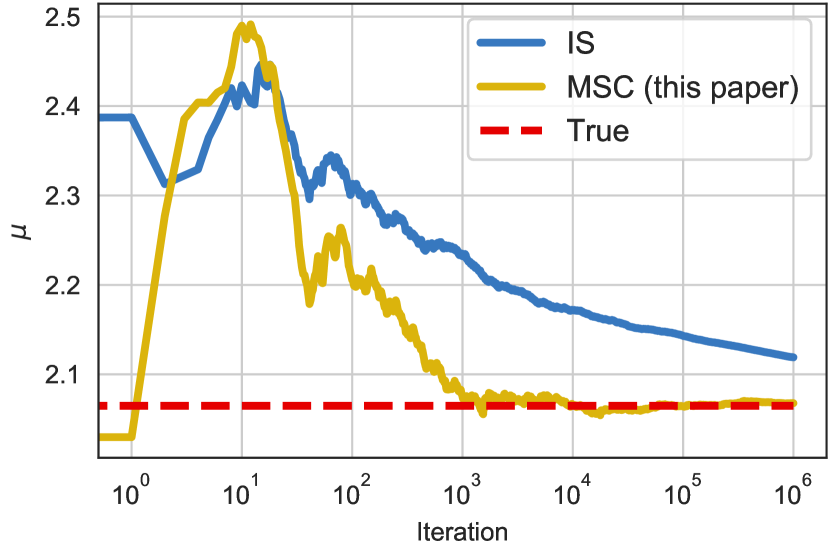
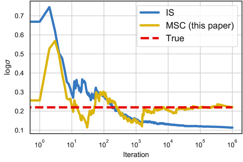
Figure 1: MSC converges to the true solution, while the biased IS approach does not. Example of learnt variational parameters for IS- and MSC-based gradients of the inclusive KL, as well as true parameters. Gaussian approximation to a skew normal distribution. Iterations in log-scale.

Note that the biased IS-gradients results in an underestimation of the variance. One of the main motivations for using inclusive KL as optimization objective is to avoid such underestimation of uncertainty. This example shows that when the inclusive KL is optimized with biased gradients the solution can no longer be trusted in this respect. The gradients for Rényi- and $\chi$ divergences used in e.g. [35, 15] suffer from a similar bias. The supplement provides a $\chi$ divergence analogue to fig. 1.

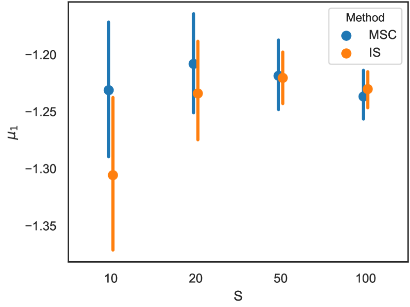
(a) Heart $\mu_{1}^{\star}$

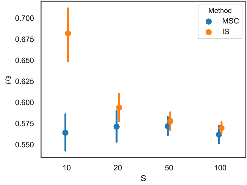
(b) Heart $\mu_{3}^{\star}$

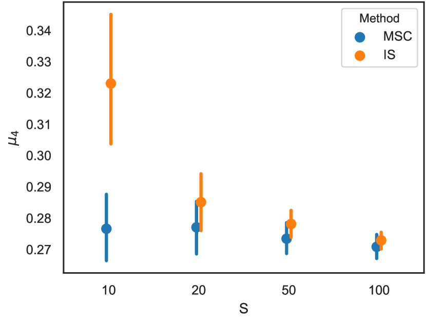
(c) Heart $\mu_{4}^{\star}$

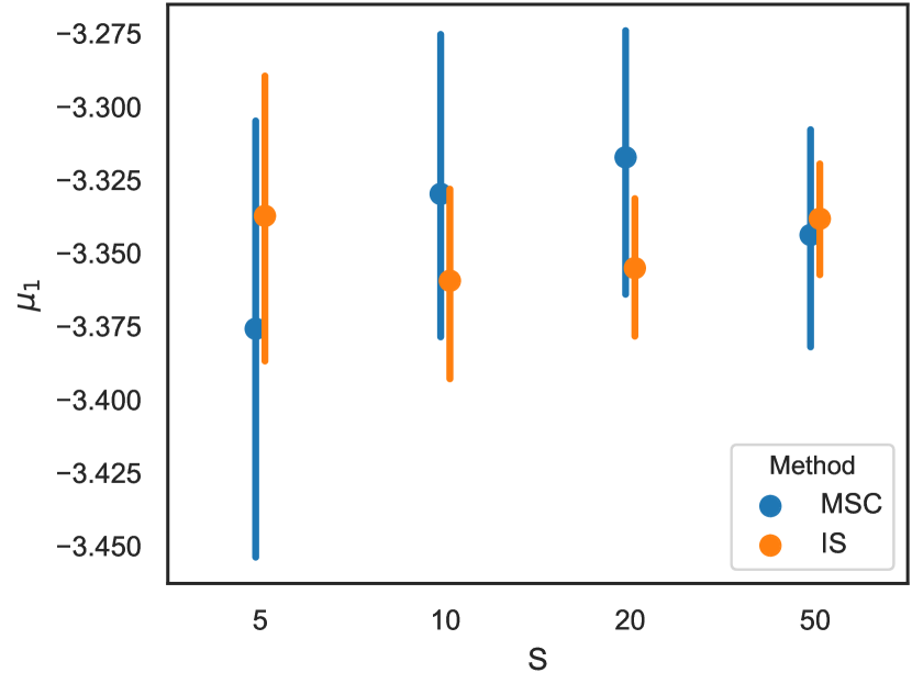
(d) Ionos $\mu_{1}^{\star}$

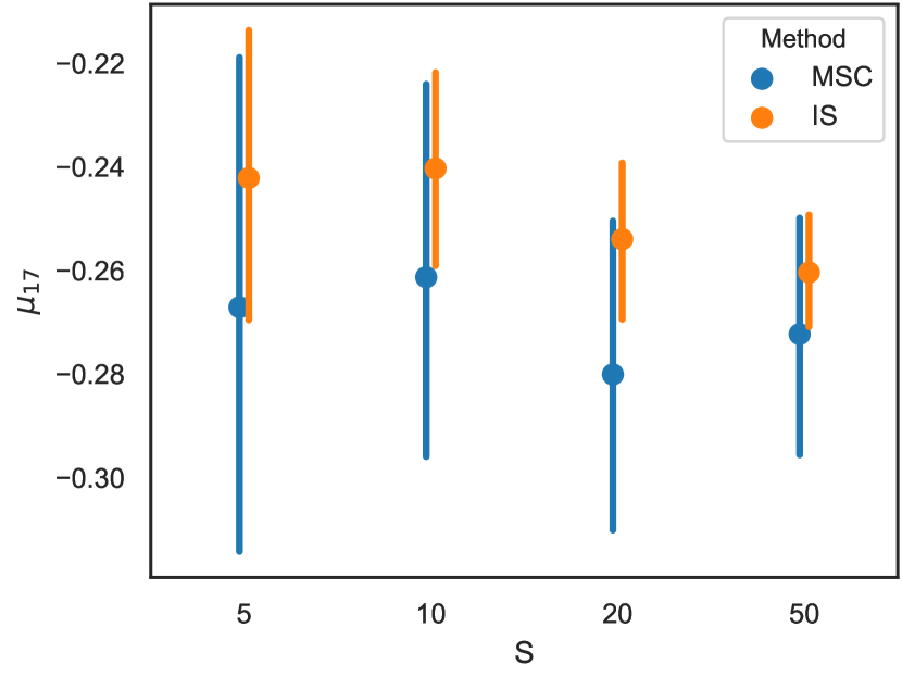
(e) Ionos $\mu_{17}^{\star}$

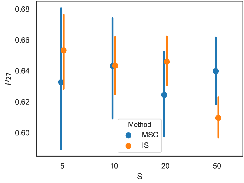
(f) Ionos $\mu_{27}^{\star}$

Figure 2: MSC is more robust to the number of samples $S$. The fitted mean parameter $\mu^{\star}$, for three representative dimensions of $\mathbf{z}$, of MSC (this paper) and IS (cf. [7]) on the Ionos and Heart datasets. The error bars corresponds to $100$ random initializations.

4.2 Bayesian Probit Regression

Probit regression is commonly used for binary classification in machine learning and statistics. The Bayesian probit regression model assigns a Gaussian prior to the parameters. The prior and likelihood are $p(\mathbf{z})=\mathcal{N}\left(\mathbf{z}\,;\,0,I\right)$, $\mathbb{P}(\mathbf{y}_{t}=y\,|\,\mathbf{z},\mathbf{x}_{t})=\Phi(\mathbf{x}_{t}^{\top}\mathbf{z})^{y}\left(1-\Phi(\mathbf{x}_{t}^{\top}\mathbf{z})\right)^{1-y}$, where $y\in\{0,1\}$ and $\Phi(\cdot)$ is the cumulative distribution function of the normal distribution. We apply the model for prediction in several UCI datasets [18]. We let the variational approximation be a Gaussian distribution $q(\mathbf{z}\,;\,\lambda)=\mathcal{N}\left(\mathbf{z}\,;\,\mu,\Sigma\right)$, where $\Sigma$ is a diagonal covariance matrix. We compare MSC (this paper) with the biased IS-based approach (cf. eq. 6 and [7]) and EP [43] that minimizes the inclusive KL locally. For SGD methods we use adaptive step-sizes [29].

Table 1 illustrates the predictive performance of the fitted model on held-out test data. The results where generated by splitting each dataset $100$ times into $90\%$ training and $10\%$ test data, then computing average prediction error and its standard deviation. MSC performs as well as EP which is particularly well suited to this problem. However, EP requires more model-specific derivations and can be difficult to implement when the moment matching subproblem can not be solved in closed form. In these experiments the bias introduced by IS does not significantly impact the predictive performance compared to MSC.

Dataset	EP [43]	IS [7]	MSC (adaptive)	MSC (prior)
Pima	$0.227\pm 0.048$	$0.229\pm 0.047$	$0.227\pm 0.046$	$0.456\pm 0.093$
Ionos	$0.115\pm 0.053$	$0.115\pm 0.054$	$0.117\pm 0.053$	$0.182\pm 0.070$
Heart	$0.161\pm 0.066$	$0.163\pm 0.066$	$0.160\pm 0.063$	$0.342\pm 0.11$

Table 1: Test error for Bayesian probit regression; lower is better. Estimated using EP [43], IS (cf. [7]), and MSC (this paper) with proposal $q(\mathbf{z}\,;\,\lambda)$ (adaptive) or $p(\mathbf{z})$ (prior) for $3$ UCI datasets. Predictive performance is comparable, but MSC is more robust and generically applicable.

We compare how the approximations based on MSC and IS are affected by the number of samples $S$ at each iteration. In fig. 2 we plot the mean value $\mu^{\star}$ based on $100$ random initializations for several values of $S$ on the Heart and Ionos datasets. The MSC is more robust to the choice of $S$, converging to similar mean values for all the choices of $S$ in this example. For the Heart dataset, IS clearly struggles with a bias for low values of the number of samples $S$.

4.3 Stochastic Volatility

The stochastic volatility model is commonly used in financial econometrics [12]. The model is $p(\mathbf{z}_{0}\,;\,\theta)=\mathcal{N}\left(\mathbf{z}_{0}\,;\,0,\frac{\sigma^{2}}{1-\phi^{2}}\right),\quad p(\mathbf{z}_{t}\,|\,\mathbf{z}_{t-1}\,;\,\theta)=\mathcal{N}\left(\mathbf{z}_{t}\,;\,\mu+\phi(\mathbf{z}_{t-1}-\mu),\sigma^{2}\right)$, $p(\mathbf{x}_{t}\,|\,\mathbf{z}_{t}\,;\,\theta)=\mathcal{N}\left(\mathbf{x}_{t}\,;\,0,\beta\exp(\mathbf{z}_{t})\right)$, where the parameters are constrained as follows $\theta=\left(\sigma^{2},\phi,\mu,\beta\right)\in\mathbb{R}_{+}\times(-1,1)\times\mathbb{R}\times\mathbb{R}_{+}$. Both the posterior distribution and log-marginal likelihood are intractable so we make use of algorithm 3 as outlined in section 3.3 with the CSMC kernel described in the supplement. The proposal distributions are $q(\mathbf{z}_{0}\,;\,\theta,\lambda_{0})\propto p(\mathbf{z}_{0}\,;\,\theta)e^{-\frac{1}{2}\Lambda_{0}\mathbf{z}_{0}^{2}+\nu_{0}\mathbf{z}_{0}}$, $q(\mathbf{z}_{t}\,|\,\mathbf{z}_{t-1}\,;\,\theta,\lambda_{t})\propto p(\mathbf{z}_{t}\,|\,\mathbf{z}_{t-1}\,;\,\theta)\,e^{-\frac{1}{2}\Lambda_{t}\mathbf{z}_{t}^{2}+\nu_{t}\mathbf{z}_{t}}$, with variational parameters $\lambda_{t}=(\nu_{t},\Lambda_{t})\in\mathbb{R}\times\mathbb{R}_{+}$.

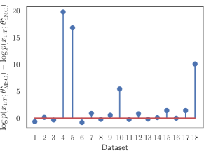
Figure 3: Difference in log-marginal likelihood values for parameters learnt by MSC (this paper) and SMC [22]. The likelihood obtained by MSC, on average, is superior to or as good as that obtained by SMC.

We compare MSC with the SMC-based approach [22] using adaptive step-size [29]. We study monthly returns over $10$ years ($9/2007$ to $8/2017$) for the exchange rate of $18$ currencies with respect to the US dollar. The data is obtained from the Federal Reserve System. In fig. 3 we illustrate the difference between the log-marginal likelihood obtained by the two methods, $\log p(\mathbf{x}\,;\,\theta_{\textrm{MSC}}^{\star})-\log p(\mathbf{x}\,;\,\theta_{\textrm{SMC}}^{\star})$. We learn the model and variational parameters using $S=10$ particles for both methods, and estimate the log-marginal likelihood after convergence using $S=10,000$. The log-marginal likelihood obtained by MSC is significantly better than SMC for several of the datasets.

5 Conclusions

In VI, the properties of the approximation $q$, to the posterior $p$, depends on the choice of divergence that is minimized. The most common choice is the exclusive KL divergence $\textrm{KL}\left(q\;\|\;p\right)$, which is computationally convenient, but known to suffer from underestimation of the posterior uncertainty. An alternative, which has been our focus here, is the inclusive KL divergence $\textrm{KL}\left(p\;\|\;q\right)$. The benefit of using the inclusive KL is to obtain a more “robust” approximation that does not underestimate the uncertainty. However, in this paper we have argued, and illustrated numerically, that such underestimation of uncertainty can still be an issue, if the optimization is based on biased gradient estimates, as is the case for previously proposed VI algorithms. As a remedy, we introduced Markovian score climbing, a new way to reliably learn a variational approximation that minimizes the inclusive KL. This results in a method that melds VI and MCMC. We have illustrated its convergence properties on a simple toy example, and studied its performance on Bayesian probit regression for classification as well as a stochastic volatility model for financial data.

Broader Impact

MSC is a general purpose approximate statistical inference method. The main goal is to remove systematic errors due to biased estimates of the gradient of the optimization objective function. This can allow for more reliable and robust inferences based on the posterior approximation. However, just like other standard inference methods it does not protect from any bias introduced by applying it to specific models and data [13, 41].

Appendix A Supplementary Material

A.1 Subset Average Likelihood

Li and Turner [35], Dieng et al. [15], who study different classes of divergences where the likelihood also enters as a product, propose to replace the true likelihood at each iteration with a “subset average likelihood”. The subset average likelihood approach makes the following approximation

$$p(\mathbf{x}\,|\,\mathbf{z})=\prod_{i=1}^{n}p(x_{i}\,|\,\mathbf{z})\approx p(\mathbf{x}_{M}\,|\,\mathbf{z})^{\frac{n}{m}}:=\prod_{j\in M}p(x_{j}\,|\,\mathbf{z})^{\frac{n}{m}},$$

where $M\subset\{1,\ldots,n\}$ is a set of indices corresponding to a mini-batch of size $m=|M|$ data points sampled uniformly from $\{x_{1},\ldots,x_{n}\}$ with or without replacement. Considering the same approach for the inclusive KL case the unbiased stochastic gradient obtained is

$$\frac{1}{S}\sum_{s=1}^{S}\frac{p(\mathbf{z}^{s})p(\mathbf{x}_{M}\,|\,\mathbf{z}^{s})^{\frac{n}{m}}}{q(\mathbf{z}^{s}\,;\,\lambda)}\nabla_{\lambda}\log q(\mathbf{z}^{s}\,;\,\lambda),\leavevmode\nobreak\ \mathbf{z}^{s}\sim q(\mathbf{z}\,;\,\lambda).$$ (9)

This approximation also leads to a systematic error in the SGD algorithm. It is no longer minimizing the KL divergence from the posterior $p$ to the variational approximation $q$. In fact, it is possible to show that it is actually minimizing the KL divergence from a perturbed posterior $\widetilde{p}$, where the likelihood is replaced by a mixture of all potential subset average likelihoods, to the variational approximation $q$. This result is formalized by 2.

Proposition 2.

Using the stochastic gradient defined by eq. 9 and an iterative SGD algorithm according to eq. 4 the fixed points $\lambda^{\star}$ are identical to the solution to

$$\nabla_{\lambda}\mathrm{KL}\left(\widetilde{p}(\mathbf{z}\,|\,\mathbf{x})\|q(\mathbf{z}\,;\,\lambda)\right)=0,$$ (10)

where the perturbed posterior $\widetilde{p}$, if it exists, is given by

$$\widetilde{p}(\mathbf{z}\,|\,\mathbf{x}) \propto p(\mathbf{z})\sum_{M\in\mathcal{M}}p(\mathbf{x}_{M}\,|\,\mathbf{z})^{\frac{n}{m}},$$

and $\mathcal{M}$ is the set of all possible combinations of mini-batches $M$ of size $m$.

Proof.

See the Supplementary Material. ∎

In the supplement we provide illustrations on a simulated example. It is in general difficult to determine the magnitude of the error introduced by the subset average likelihood in practical applications. The subset average likelihood approach for Rényi and $\chi^{2}$ divergences [35, 15] likewise leads to a systematic error in the stochastic gradient. Furthermore, the fixed points of the resulting stochastic systems for these divergences are difficult to quantify, making it even harder to understand the effect of the approximation.

Conditional Sequential Monte Carlo

Just like CIS is a straightforward modification of IS, so is CSMC a straightforward modification of SMC. We make use of CSMC with ancestor sampling as proposed by Lindsten et al. [38] combined with twisted SMC [23, 25, 47]. While SMC can be adapted to perform inference for almost any probabilistic model [47], we here focus on the state space model

$$p(\mathbf{z}_{1:T},\mathbf{x}_{1:T}) =p(\mathbf{z}_{1})p(\mathbf{x}_{1}\,|\,\mathbf{z}_{1})\prod_{t=1}^{T}p(\mathbf{z}_{t}\,|\,\mathbf{z}_{t-1})p(\mathbf{x}_{t}\,|\,\mathbf{z}_{t}),$$

where we assume that the prior $p(\mathbf{z}_{1})$ and transition $p(\mathbf{z}_{t}\,|\,\mathbf{z}_{t-1})$ are conditionally Gaussian. Because the prior and transition distributions are Gaussian it is convenient to define the full approximation to the posterior $p(\mathbf{z}_{1:T}\,|\,\mathbf{x}_{1:T})$ to be the multivariate normal

$$q(\mathbf{z}_{1:T}\,;\,\lambda) =q(\mathbf{z}_{1}\,;\,\lambda_{1})\prod_{t=2}^{T}q(\mathbf{z}_{t}\,|\,\mathbf{z}_{t-1}\,;\,\lambda_{t}),$$ (11)

$$q(\mathbf{z}_{1}\,;\,\lambda_{1}) \propto p(\mathbf{z}_{1})\psi(\mathbf{z}_{1}\,;\,\lambda_{1}),$$

$$q(\mathbf{z}_{t}\,|\,\mathbf{z}_{t-1}\,;\,\lambda_{t}) \propto p(\mathbf{z}_{t}\,|\,\mathbf{z}_{t-1})\psi(\mathbf{z}_{t}\,;\,\lambda_{t}),$$

where $\psi$ are twisting potentials

$$\psi(\mathbf{z}_{t}\,;\,\lambda_{t}) =\exp\left(-\frac{1}{2}\mathbf{z}_{t}^{\top}\Lambda_{t}\mathbf{z}_{t}+\nu_{t}^{\top}\mathbf{z}_{t}\right),$$

with $\lambda_{t}=(\Lambda_{t},\nu_{t})$. We are now equipped to explain the CSMC kernel that updates a conditional trajectory $\mathbf{z}_{1:T}[k-1]=(\mathbf{z}_{1}[k-1],\ldots\mathbf{z}_{T}[k-1])$. Each iteration of CSMC consists of three steps: initialization for $t=1$, running a modified SMC algorithm for $t>1$, and then updating the conditional sample for the next iteration. We explain in detail below.

First, perform (conditional) IS for the first step where $t=1$. Set $\mathbf{z}_{1}^{1}=\mathbf{z}_{1}[k-1]$ and propose the remaining $S-1$ samples from a proposal distribution $q$

$$\mathbf{z}_{1}^{i} \sim q(\mathbf{z}_{1}\,;\,\lambda_{1}),\quad i=2,\ldots,S$$

and compute the importance weights for $i=1,\ldots,S$

$$w_{1}^{i} =\frac{p(\mathbf{z}_{1}^{i})\psi(\mathbf{z}_{1}^{i}\,;\,\lambda_{1})}{q(\mathbf{z}_{1}^{i}\,;\,\lambda_{1})}, \bar{w}_{1}^{i}=\frac{w_{1}^{i}}{\sum_{j=1}^{S}w_{1}^{j}}.$$

Then, for each step $t>1$ in turn perform resampling, ancestor sampling, propagation and weighting. Resampling picks the most promising earlier sample to propagate, i.e. for $i=2,\ldots,S$ simulate ancestor variables $a_{t-1}^{i}$ with probability

$$\mathbb{P}\left(a_{t-1}^{i}=j\right) =\bar{w}_{t-1}^{j}.$$

For $i=1$ instead, simulate the corresponding ancestor variable $a_{t-1}^{1}$ with probability

$$\mathbb{P}\left(a_{t-1}^{1}=j\right) \propto\bar{w}_{t-1}^{j}q(\mathbf{z}_{t}[k-1]\,|\,\mathbf{z}_{t-1}^{j}\,;\,\lambda_{t}),$$

where $\mathbf{z}_{t}[k-1]$ is the corresponding element of the conditional trajectory $\mathbf{z}_{1:T}$ from the previous iteration. This is known as ancestor sampling [38].

When propagating for $i=1$ simply set $\mathbf{z}_{t}^{1}=\mathbf{z}_{t}[k-1]$, and simulate the remainder from the proposal distribution

$$\mathbf{z}_{t}^{i} \sim q(\mathbf{z}_{t}\,|\,\mathbf{z}_{t-1}^{a_{t-1}^{i}}\,;\,\lambda),\quad i=2,\ldots,S$$

Set $\mathbf{z}_{1:t}^{i}=(\mathbf{z}_{1:t-1}^{a_{t-1}^{i}},\mathbf{z}_{t}^{i})$ and compute the weights for all $i=1,\ldots,S$

$$w_{t}^{i} =\frac{p(\mathbf{z}_{t}^{i}\,|\,\mathbf{z}_{t-1}^{a_{t-1}^{i}})p(\mathbf{x}_{t-1}\,|\,\mathbf{z}_{t-1}^{a_{t-1}^{i}})}{q(\mathbf{z}_{t}^{i}\,|\,\mathbf{z}_{t-1}^{a_{t-1}^{i}}\,;\,\lambda_{t})}\frac{\psi(\mathbf{z}_{t}^{i}\,;\,\lambda_{t})}{\psi(\mathbf{z}_{t-1}^{a_{t-1}^{i}}\,;\,\lambda_{t-1})},$$ (12)

$$\bar{w}_{t}^{i} =\frac{w_{t}^{i}}{\sum_{j=1}^{S}w_{t}^{j}}.$$

For the final step $t=T$ the (unnormalized) weights are instead

$$w_{T}^{i} =\frac{p(\mathbf{z}_{T}^{i}\,|\,\mathbf{z}_{T-1}^{a_{T-1}^{i}})p(\mathbf{x}_{T-1}\,|\,\mathbf{z}_{T-1}^{a_{T-1}^{i}})}{q(\mathbf{z}_{T}^{i}\,|\,\mathbf{z}_{T-1}^{a_{T-1}^{i}}\,;\,\lambda_{T})}\frac{p(\mathbf{x}_{T}\,|\,\mathbf{z}_{T}^{i})}{\psi(\mathbf{z}_{t-1}^{a_{t-1}^{i}}\,;\,\lambda_{t-1})}.$$ (13)

Finally, an updated conditional sample is generated by picking one of the proposed trajectories with probability proportional to its (normalized) weight, i.e.

$$\mathbf{z}_{1:T}[k] =\mathbf{z}_{1:T}^{J},\quad$$

where $J$ is a discrete random variable with probability $\mathbb{P}(J=j)=\bar{w}_{T}^{j}$.

Repeating this procedure iteratively constructs a Markov chain with the posterior $p(\mathbf{z}_{1:T}\,|\,\mathbf{x}_{1:T})$ as its stationary distribution [2, 38, 47]. With this it is possible to attain an estimate of the gradient with respect to the variational parameters of eq. 1 as follows

$$\widehat{g}_{\textrm{KL}}(\lambda) =-\nabla_{\lambda}\log q(\mathbf{z}_{1:T}[k]\,;\,\lambda),$$ (14)

where $\mathbf{z}_{1:T}[k]$ is the conditional sample retained at iteration $k$ of the CSMC algorithm.

We summarize one full iteration of the CSMC algorithm in algorithm 4. This algorithm defines a Markov kernel $M(\mathbf{z}_{1:T}[k]\,|\,\mathbf{z}_{1:T}[k-1]\,;\,\lambda)$ useful for MSC.

Input : Model $p(\mathbf{z}_{1:T},\mathbf{x}_{1:T})$, proposal $q(\mathbf{z}_{1:T}\,;\,\lambda)$, conditional sample $\mathbf{z}_{1:T}[k-1]$, and total number of internal samples $S$.

Output : $\mathbf{z}_{1:T}[k]\sim M(\cdot\,|\,\mathbf{z}_{1:T}[k-1]\,;\,\lambda)$, updated conditional sample.

1 Set $\displaystyle\mathbf{z}_{1}^{1}=\mathbf{z}_{1}[k]$

2

3Sample $\displaystyle\mathbf{z}_{1}^{i}\sim q(\mathbf{z}_{1}\,;\,\lambda_{1})$ for $\displaystyle i=2,\ldots,S$

4

5Compute $\displaystyle w_{1}^{i}=\frac{p(\mathbf{z}_{1}^{i})\psi(\mathbf{z}_{1}^{i}\,;\,\lambda_{1})}{q(\mathbf{z}_{1}^{i}\,;\,\lambda_{1})}$ for $\displaystyle i=1,\ldots,S$

6

7for $\displaystyle t=2,\ldots,T$ do

8       for $\displaystyle i=2,\ldots,S$ do

9             Sample $a_{t-1}^{i}$ w.p. $\mathbb{P}(a_{t-1}^{i}=j)=\bar{w}_{t-1}^{j}$

10            

11            Sample $\mathbf{z}_{t}^{i}\sim q(\mathbf{z}_{t}\,|\,\mathbf{z}_{t-1}^{a_{t-1}^{i}}\,;\,\lambda_{t})$

12            

13       end for

14      Sample $a_{t-1}^{1}$ w.p.

15      $\mathbb{P}(a_{t-1}^{i}=j)\propto\bar{w}_{t-1}^{j}q(\mathbf{z}_{t}[k]\,|\,\mathbf{z}_{t-1}^{j}\,;\,\lambda_{t})$

16      

17      Set $\mathbf{z}_{t}^{1}=\mathbf{z}_{t}[k]$

18      

19      for $\displaystyle i=1,\ldots,S$ do

20             Compute $w_{t}^{i}$ in eq. 12 or eq. 13

21            

22            Set $\mathbf{z}_{1:t}^{i}=\left(\mathbf{z}_{1:t-1}^{a_{t-1}^{i}},\mathbf{z}_{t}^{i}\right)$

23       end for

24      

25 end for

26

27Sample $\displaystyle J$ with probability $\displaystyle\mathbb{P}(J=j)\propto\bar{w}_{T}^{j}$

28

29Set $\displaystyle\mathbf{z}_{1:T}[k]=\mathbf{z}_{1:T}^{J}$

Algorithm 4 Conditional Sequential Monte Carlo

Proof of Proposition 1

This result is an adaptation of Gu and Kong [21, Theorem 1] based on Benveniste et al. [5, Theorem 3.17, page 304]. Let $\lambda^{\star}$ be a minimizer of the inclusive KL divergence in eq. 1. Consider the ordinary differential equation (ODE) defined by

$$\frac{\mathop{}\!\mathrm{d}}{\mathop{}\!\mathrm{d}t}\lambda(t) =\mathbb{E}_{p(\mathbf{z}\,|\,\mathbf{x})}\left[-s(\mathbf{z}\,;\,\lambda(t))\right],\quad\lambda(0)=\lambda_{0},$$ (15)

and its solution $\lambda(t)$, $t\geq 0$. If the ODE in eq. 15 admits the unique solution $\lambda(t)=\widehat{\lambda}$, $t\geq 0$ for $\lambda(0)=\widehat{\lambda}$, then $\widehat{\lambda}$ is called a stability point. The minimzer $\lambda^{\star}$ is a stability point of eq. 15. A set $\Lambda$ is called the domain of attraction of $\widehat{\lambda}$, if the solution to eq. 15 for $\lambda(0)\in\Lambda$ remains in $\Lambda$ and converges to $\widehat{\lambda}$. Suppose that $\lambda_{k}\in\mathbb{R}^{d}$ and that $\Lambda$ is an open set in $\mathbb{R}^{d_{\lambda}}$. Furthermore, suppose $\mathbf{z}[k]\in\mathbb{R}^{d_{z}}$ and that $Z$ is an open set in $\mathbb{R}^{d_{z}}$. Denote the Markov kernel in MSC, algorithm 1, by $M_{\lambda}(\mathbf{z},\mathop{}\!\mathrm{d}\mathbf{z}^{\prime})$ and repeated application of it by $M_{\lambda}^{k}(\mathbf{z},\mathop{}\!\mathrm{d}\mathbf{z}^{\prime})=\int\cdots\int M_{\lambda}(\mathbf{z},\mathop{}\!\mathrm{d}\mathbf{z}_{1})M_{\lambda}(\mathbf{z}_{2},\mathop{}\!\mathrm{d}\mathbf{z}_{3})\cdots M_{\lambda}(\mathbf{z}_{k-1},\mathop{}\!\mathrm{d}\mathbf{z}^{\prime})$. $|\mathbf{z}|$ denotes the length of the vector $\mathbf{z}$. Let $Q$ be any compact subset of $\Lambda$, and $q>1$ a sufficiently large real number such that the following assumptions hold. We follow Gu and Kong [21] and assume:

C 1.

Assume that the step size sequence satisfies $\sum_{k=1}^{\infty}\varepsilon_{k}=\infty$ and $\sum_{k=1}^{\infty}\varepsilon_{k}^{2}<\infty$.

C 2 (Integrability).

There exists a constant $C_{1}$ such that for any $\lambda\in\Lambda$, $\mathbf{z}\in Z$ and $k\geq 1$,

$$\int\left(1+|\mathbf{z}^{\prime}|^{q}\right)M_{\lambda}^{k}(\mathbf{z},\mathop{}\!\mathrm{d}\mathbf{z}^{\prime})\leq C_{1}\left(1+|\mathbf{z}|^{q}\right)$$

C 3 (Convergence of the Markov Chain).

Let $p(\mathbf{z}\,|\,\mathbf{x})$ be the unique invariant measure for $M_{\lambda}$. For each $\lambda\in\Lambda$,

$$\lim_{k\to\infty}\sup_{\mathbf{z}\in Z}\frac{1}{1+|\mathbf{z}|^{q}}\int\left(1+|\mathbf{z}^{\prime}|^{q}\right)|M_{\lambda}^{k}(\mathbf{z},\mathop{}\!\mathrm{d}\mathbf{z}^{\prime})-p(\mathop{}\!\mathrm{d}\mathbf{z}^{\prime}\,|\,\mathbf{x})|=0.$$

C 4 (Continuity in $\lambda$).

There exists a constant $C_{2}$, such that for all $\lambda,\lambda^{\prime}\in Q$

$$\left|\int\left(1+|\mathbf{z}^{\prime}|^{q}\right)\left(M_{\lambda}(\mathbf{z},\mathop{}\!\mathrm{d}\mathbf{z}^{\prime})-M_{\lambda^{\prime}}(\mathbf{z},\mathop{}\!\mathrm{d}\mathbf{z}^{\prime})\right)\right|\leq C_{2}|\lambda-\lambda^{\prime}|\left(1+|\mathbf{z}|^{q}\right).$$

C 5 (Continuity in $\mathbf{z}$).

There exists a constant $C_{3}$, such that for all $\mathbf{z}_{1},\mathbf{z}_{2}\in Z$

$$\sup_{\lambda\in\Lambda}\left|\int\left(1+|\mathbf{z}^{\prime}|^{q+1}\right)\left(M_{\lambda}(\mathbf{z}_{1},\mathop{}\!\mathrm{d}\mathbf{z}^{\prime})-M_{\lambda}(\mathbf{z}_{2},\mathop{}\!\mathrm{d}\mathbf{z}^{\prime})\right)\right|\leq C_{3}|\mathbf{z}_{1}-\mathbf{z}_{2}|\left(1+|\mathbf{z}_{1}|^{q}+|\mathbf{z}_{2}|^{q}\right).$$

C 6 (Conditions on the Score Function).

For any compact subset $Q\subset\Lambda$, there exist positive constants $p$, $K_{1}$, $K_{2}$, $K_{3}$ and $\nu>\nicefrac{{1}}{{2}}$ such that for all $\lambda,\lambda^{\prime}\in\Lambda$ and $\mathbf{z},\mathbf{z}_{1},\mathbf{z}_{2}\in Z$,

$$|\nabla_{\lambda}\log q(\mathbf{z}\,;\,\lambda)| \leq K_{1}\left(1+|\mathbf{z}|^{p+1}\right),$$

$$|\nabla_{\lambda}\log q(\mathbf{z}_{1}\,;\,\lambda)-\nabla_{\lambda}\log q(\mathbf{z}_{2}\,;\,\lambda)| \leq K_{2}|\mathbf{z}_{1}-\mathbf{z}_{2}|\left(1+|\mathbf{z}_{1}|^{p}+|\mathbf{z}_{2}|^{p}\right),$$

$$|\nabla_{\lambda}\log q(\mathbf{z}\,;\,\lambda)-\nabla_{\lambda}\log q(\mathbf{z}\,;\,\lambda^{\prime})| \leq K_{3}|\lambda-\lambda^{\prime}|^{\nu}\left(1+|\mathbf{z}|^{p+1}\right).$$

The constants $C_{1},\ldots,C_{3}$ and $\nu$ may depend on the compact set $Q$ and the real number $q$. 1 is the standard Robbins-Monro condition and 6 controls the regularity of the model. 2-5 have to do with the convergence and continuity of the Markov kernel. These conditions can be difficult to verify in the general case, but can be proven more easily under the simplifying assumption that Z is compact. See Lindholm and Lindsten [37, Appendix B] for a proof of continuity of the CSMC kernel, which can also be adapted to the CIS kernel.

With the above assumptions the result follows from Gu and Kong [21, Theorem 1] where (left - their notation, right - our notation)

$$\theta =\lambda,$$

$$x =\mathbf{z},$$

$$\Pi_{\theta} =M_{\lambda},$$

$$H(\theta,x) =\nabla_{\lambda}\log q(\mathbf{z}\,;\,\lambda),$$

and $I(\theta,x)=0$, $\Gamma_{k}=0$.

Proof of Proposition 2

The fixed points of the iterative algorithm are the solutions to the equation when we set the expectation of eq. 9 equal to zero. The equation is given by

$$\mathbb{E}\left[-\frac{1}{S}\sum_{s=1}^{S}\frac{p(\mathbf{z}^{s})p(\mathbf{x}_{M}\,|\,\mathbf{z}^{s})^{\frac{n}{m}}}{q(\mathbf{z}^{s}\,;\,\lambda)}\nabla_{\lambda}\log q(\mathbf{z}^{s}\,;\,\lambda)\right]=\mathbb{E}\left[-\frac{p(\mathbf{z})p(\mathbf{x}_{M}\,|\,\mathbf{z})^{\frac{n}{m}}}{q(\mathbf{z}\,;\,\lambda)}\nabla_{\lambda}\log q(\mathbf{z}\,;\,\lambda)\right]$$

$$=\mathbb{E}\left[-\frac{p(\mathbf{z})\frac{1}{|\mathcal{M}|}\sum_{M\in\mathcal{M}}p(\mathbf{x}_{M}\,|\,\mathbf{z})^{\frac{n}{m}}}{q(\mathbf{z}\,;\,\lambda)}\nabla_{\lambda}\log q(\mathbf{z}\,;\,\lambda)\right]=0$$

$$\Longleftrightarrow\mathbb{E}_{\widetilde{p}(\mathbf{z}\,|\,\mathbf{x})}\left[-\nabla_{\lambda}\log q(\mathbf{z}\,;\,\lambda)\right]=0$$

$$\Longleftrightarrow\nabla_{\lambda}\mathrm{KL}\left(\widetilde{p}(\mathbf{z}\,|\,\mathbf{x})\|q(\mathbf{z}\,;\,\lambda)\right)=0,$$

where the first equality follows because the samples $\mathbf{z}^{s}$ are independent and identically distributed. The second equality follows by the distribution of the mini-batches. The first equivalence follows because $\mathbf{z}\sim q(\mathbf{z}\,;\,\lambda)$ and we multiply both sides by a constant independent of $\lambda$. The final equivalence follows because $\widetilde{p}(\mathbf{z}\,|\,\mathbf{x})$ does not depend on $\lambda$. This concludes the proof.

Additional Results Bayesian Probit Regression

We also compare the posterior uncertainty learnt using MSC and IS. Figure 4 shows difference in the log-standard deviation between the posterior approximation learnt using MSC and that using IS, i.e. $\log\sigma_{\mathrm{MSC}}^{\star}-\log\sigma_{\mathrm{IS}}^{\star}$. The figure contains one boxplot for each dimension of the latent variable and is based on data from $100$ random train-test splits. We can see that for two of the datasets, Heart and Ionos, MSC on average learns a posterior approximation with higher uncertainty. However, for the Pima dataset the IS-based method tends to learn higher variance approximations.

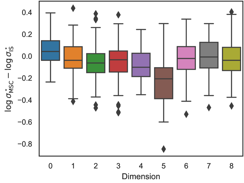
(a) Pima

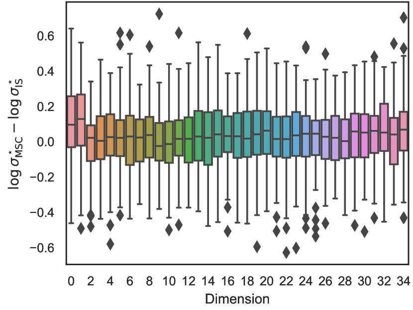
(b) Ionos

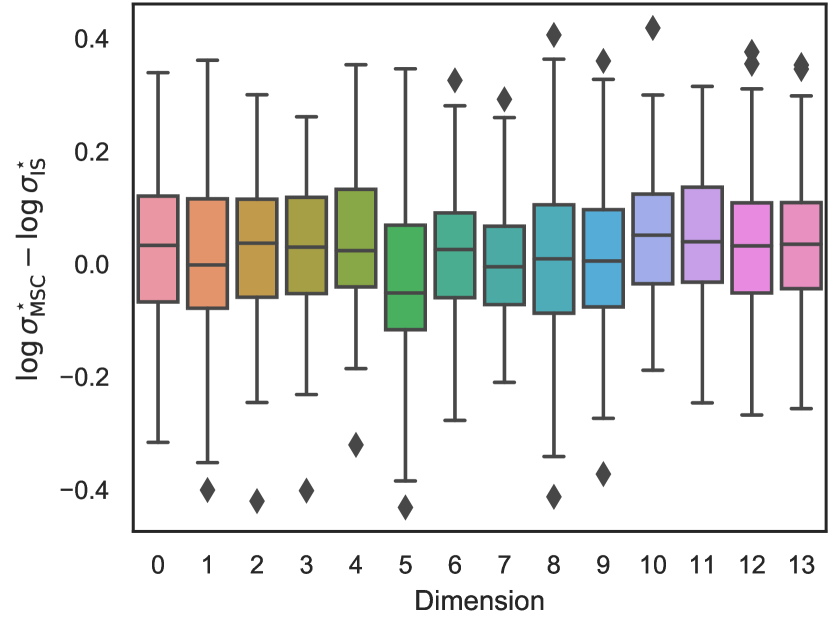
(c) Heart

Figure 4: The difference in log-standard deviation of the variational approximation, $\log\sigma_{\mathrm{MSC}}^{\star}-\log\sigma_{\mathrm{IS}}^{\star}$, between parameters learnt using MSC (this paper) and IS (cf. [7]). The dimension of the latent variable is plotted versus the parameters learnt from $100$ random splits.

Additional Results Subset Average Likelihoods

We illustrate the difference between the true and perturbed posteriors in fig. 5 for a toy example where the two distributions can be computed exactly. The model is an unknown mean measured in Gaussian noise with a conjugate prior, i.e. $\mathbf{z}\sim\mathcal{N}(0,1)$, $x_{i}\sim\mathcal{N}(\mathbf{z},1)$. To be able to exactly compute the perturbed posterior we keep the number of data points small $n=10$. The figure shows the true and perturbed posteriors for two randomly generated datasets with $m=2,5,9$.

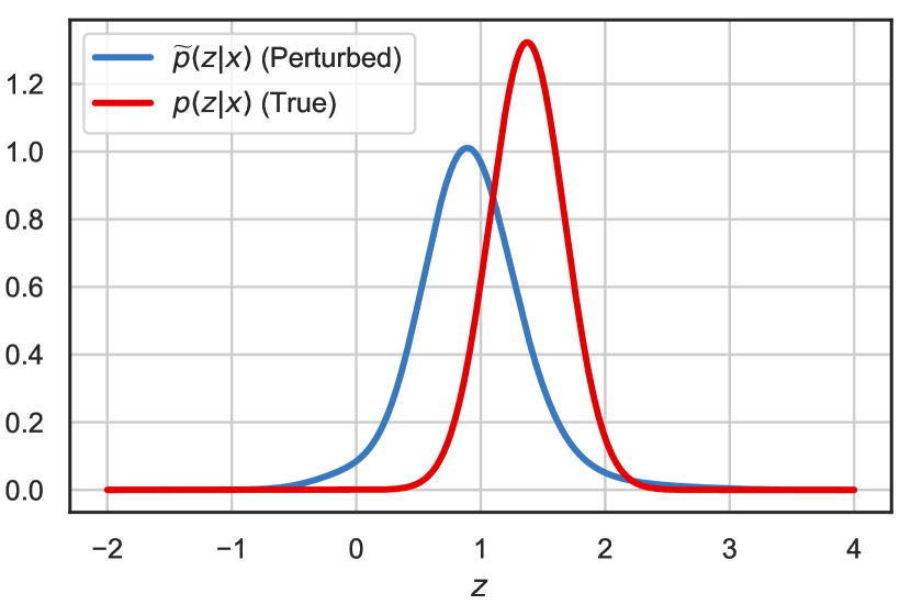
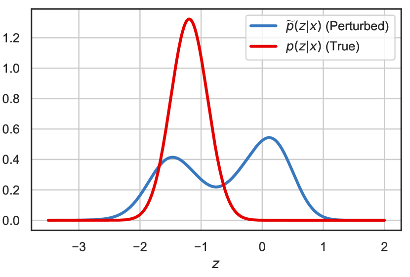
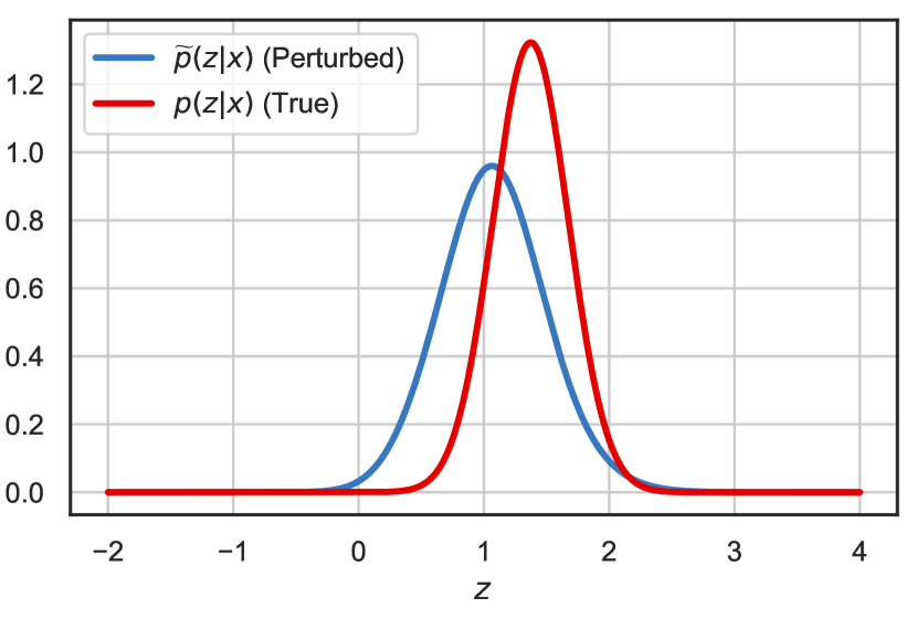
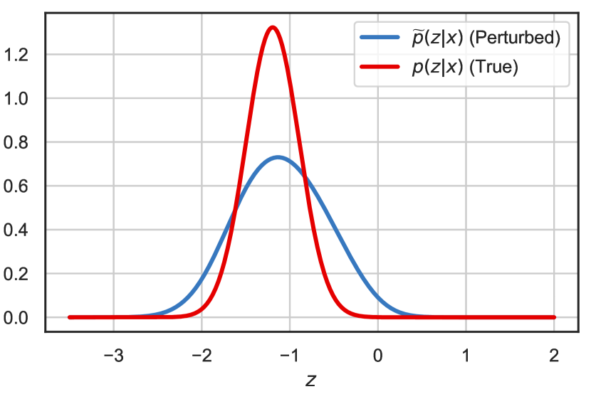
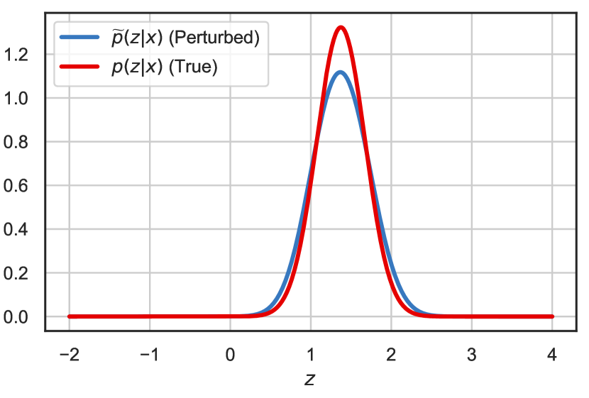
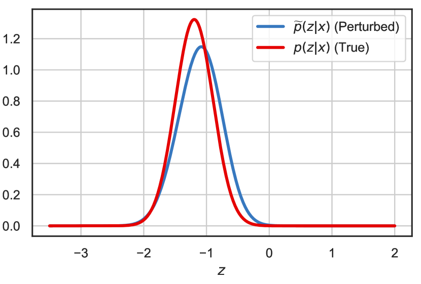
Figure 5: Example of perturbed and true posterior when using subset average likelihoods. The data used is simulated from the model defined by $\mathbf{z}\sim\mathcal{N}(0,1)$, $x_{i}\sim\mathcal{N}(\mathbf{z},1)$, $n=10$ for two different random seeds. The subset sizes where chosen to be $m=2$ (top row), $m=5$ (top row) and $m=9$ (bottom row).

Bias in $\chi$-divergence variational inference (CHIVI)

Figure 6 illustrates the systematic error introduced in the optimal parameters of CHIVI when using biased gradients.

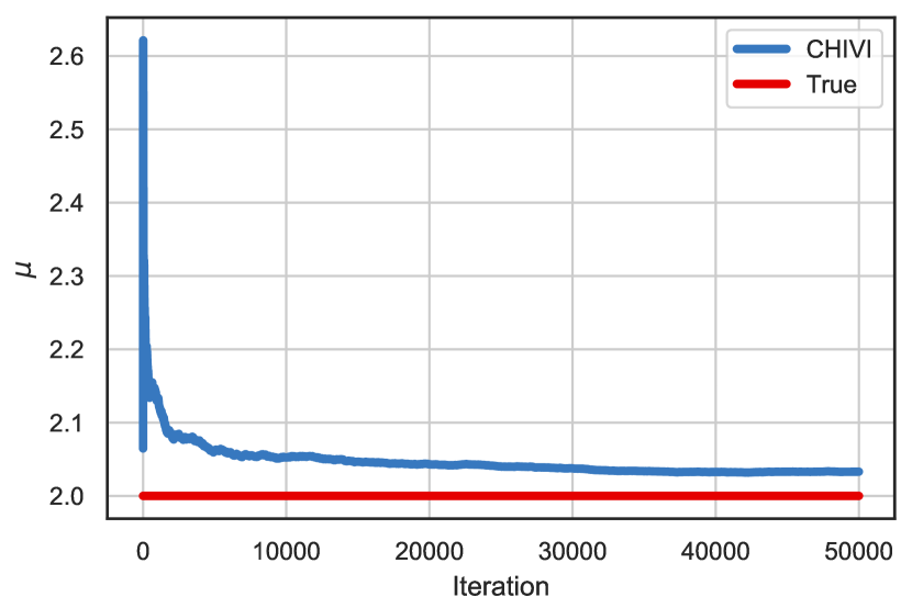
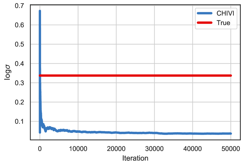
Figure 6: Example of learnt variational parameters for CHIVI, as well as true parameters when using a Gaussian approximation to a skew normal posterior distribution.

References

- Andrieu and Vihola [2014] C. Andrieu and M. Vihola. Markovian stochastic approximation with expanding projections. Bernoulli, 20(2), Nov. 2014.
- Andrieu et al. [2010] C. Andrieu, A. Doucet, and R. Holenstein. Particle Markov chain Monte Carlo methods. Journal of the Royal Statistical Society: Series B (Statistical Methodology), 72(3):269–342, 2010.
- Angelino et al. [2016] E. Angelino, M. J. Johnson, R. P. Adams, et al. Patterns of scalable Bayesian inference. Foundations and Trends® in Machine Learning, 9(2-3):119–247, 2016.
- Bardenet et al. [2017] R. Bardenet, A. Doucet, and C. Holmes. On Markov chain Monte Carlo methods for tall data. Journal of Machine Learning Research, 18(47):1–43, 2017.
- Benveniste et al. [1990] A. Benveniste, M. Métivier, and P. Priouret. Adaptive algorithms and stochastic approximations, volume 22. Springer Science & Business Media, 1990.
- Blei et al. [2017] D. Blei, A. Kucukelbir, and J. D. McAuliffe. Variational inference: A review for statisticians. Journal of the American statistical Association, 112(518):859–877, 2017.
- Bornschein and Bengio [2015] B. Bornschein and Y. Bengio. Reweighted wake-sleep. In International Conference on Learning Representations, 2015.
- Bugallo et al. [2017] M. F. Bugallo, V. Elvira, L. Martino, D. Luengo, J. Miguez, and P. M. Djuric. Adaptive importance sampling: the past, the present, and the future. IEEE Signal Processing Magazine, 34(4):60–79, 2017.
- Burda et al. [2016] Y. Burda, R. Grosse, and R. Salakhutdinov. Importance weighted autoencoders. In International Conference on Learning Representations, 2016.
- Cappé et al. [2004] O. Cappé, A. Guillin, J.-M. Marin, and C. P. Robert. Population Monte Carlo. Journal of Computational and Graphical Statistics, 13(4):907–929, 2004.
- Cappé et al. [2008] O. Cappé, R. Douc, A. Guillin, J.-M. Marin, and C. P. Robert. Adaptive importance sampling in general mixture classes. Statistics and Computing, 18(4):447–459, 2008.
- Chib et al. [2009] S. Chib, Y. Omori, and M. Asai. Multivariate Stochastic Volatility, pages 365–400. Springer Berlin Heidelberg, Berlin, Heidelberg, 2009.
- Corbett-Davies and Goel [2018] S. Corbett-Davies and S. Goel. The measure and mismeasure of fairness: A critical review of fair machine learning. arXiv:1808.00023, 2018.
- Dieng and Paisley [2019] A. B. Dieng and J. Paisley. Reweighted expectation maximization. arXiv:1906.05850, 2019.
- Dieng et al. [2017] A. B. Dieng, D. Tran, R. Ranganath, J. Paisley, and D. Blei. Variational inference via chi upper bound minimization. In Advances in Neural Information Processing Systems 30, pages 2732–2741. Curran Associates, Inc., 2017.
- Domke and Sheldon [2019] J. Domke and D. R. Sheldon. Divide and couple: Using Monte Carlo variational objectives for posterior approximation. In Advances in Neural Information Processing Systems, pages 338–347, 2019.
- Douc et al. [2007] R. Douc, A. Guillin, J.-M. Marin, C. P. Robert, et al. Convergence of adaptive mixtures of importance sampling schemes. The Annals of Statistics, 35(1):420–448, 2007.
- Dua and Graff [2017] D. Dua and C. Graff. UCI machine learning repository, 2017. URL http://archive.ics.uci.edu/ml.
- Finke and Thiery [2019] A. Finke and A. H. Thiery. On importance-weighted autoencoders. arXiv:1907.10477, 2019.
- Ghahramani and Beal [2001] Z. Ghahramani and M. J. Beal. Propagation algorithms for variational Bayesian learning. In Advances in neural information processing systems, pages 507–513, 2001.
- Gu and Kong [1998] M. G. Gu and F. H. Kong. A stochastic approximation algorithm with Markov chain Monte-Carlo method for incomplete data estimation problems. Proceedings of the National Academy of Sciences, 95(13):7270–7274, 1998.
- Gu et al. [2015] S. S. Gu, Z. Ghahramani, and R. E. Turner. Neural adaptive sequential Monte Carlo. In Advances in Neural Information Processing Systems 28, pages 2629–2637. Curran Associates, Inc., 2015.
- Guarniero et al. [2017] P. Guarniero, A. M. Johansen, and A. Lee. The iterated auxiliary particle filter. Journal of the American Statistical Association, 112(520):1636–1647, 2017.
- Habib and Barber [2019] R. Habib and D. Barber. Auxiliary variational MCMC. In International Conference on Learning Representations, 2019.
- Heng et al. [2017] J. Heng, A. N. Bishop, G. Deligiannidis, and A. Doucet. Controlled sequential Monte Carlo. arXiv:1708.08396, 2017.
- Hoffman et al. [2019] M. Hoffman, P. Sountsov, J. V. Dillon, I. Langmore, D. Tran, and S. Vasudevan. Neutra-lizing bad geometry in Hamiltonian Monte Carlo using neural transport. arXiv:1903.03704, 2019.
- Hoffman [2017] M. D. Hoffman. Learning deep latent Gaussian models with Markov chain Monte Carlo. In Proceedings of the 34th International Conference on Machine Learning, pages 1510–1519, 2017.
- Jordan et al. [1999] M. I. Jordan, Z. Ghahramani, T. S. Jaakkola, and L. K. Saul. An introduction to variational methods for graphical models. Machine Learning, 37(2):183–233, Nov. 1999.
- Kingma and Ba [2014] D. P. Kingma and J. Ba. Adam: A method for stochastic optimization. arXiv preprint arXiv:1412.6980, 2014.
- Kingma and Welling [2014] D. P. Kingma and M. Welling. Auto-encoding variational Bayes. In International Conference on Learning Representations, 2014.
- Kuhn and Lavielle [2004] E. Kuhn and M. Lavielle. Coupling a stochastic approximation version of EM with an MCMC procedure. ESAIM: Probability and Statistics, 8:115–131, 2004.
- Kushner and Yin [2003] H. Kushner and G. G. Yin. Stochastic approximation and recursive algorithms and applications, volume 35. Springer Science & Business Media, 2003.
- Lawson et al. [2018] D. Lawson, G. Tucker, C. A. Naesseth, C. Maddison, and Y. Whye Teh. Twisted variational sequential Monte Carlo. Third workshop on Bayesian Deep Learning (NeurIPS), 2018.
- Le et al. [2018] T. A. Le, M. Igl, T. Rainforth, T. Jin, and F. Wood. Auto-encoding sequential Monte Carlo. In International Conference on Learning Representations, 2018.
- Li and Turner [2016] Y. Li and R. E. Turner. Rényi divergence variational inference. In Advances in Neural Information Processing Systems 29, pages 1073–1081. Curran Associates, Inc., 2016.
- Li et al. [2017] Y. Li, R. E. Turner, and Q. Liu. Approximate inference with amortised MCMC. arXiv:1702.08343, 2017.
- Lindholm and Lindsten [2019] A. Lindholm and F. Lindsten. Learning dynamical systems with particle stochastic approximation em. arXiv:1806.09548, 2019.
- Lindsten et al. [2014] F. Lindsten, M. I. Jordan, and T. B. Schön. Particle Gibbs with ancestor sampling. The Journal of Machine Learning Research, 15(1):2145–2184, 2014.
- Lindsten et al. [2018] F. Lindsten, J. Helske, and M. Vihola. Graphical model inference: Sequential Monte Carlo meets deterministic approximations. In Advances in Neural Information Processing Systems 31, pages 8201–8211. Curran Associates, Inc., 2018.
- Maddison et al. [2017] C. J. Maddison, D. Lawson, G. Tucker, N. Heess, M. Norouzi, A. Mnih, A. Doucet, and Y. Whye Teh. Filtering variational objectives. In Advances in Neural Information Processing Systems, 2017.
- Mehrabi et al. [2019] N. Mehrabi, F. Morstatter, N. Saxena, K. Lerman, and A. Galstyan. A survey on bias and fairness in machine learning. arXiv:1908.09635, 2019.
- Minka [2005] T. Minka. Divergence measures and message passing. Technical report, Technical report, Microsoft Research, 2005.
- Minka [2001] T. P. Minka. Expectation propagation for approximate Bayesian inference. In Proceedings of the Seventeenth conference on Uncertainty in artificial intelligence, pages 362–369. Morgan Kaufmann Publishers Inc., 2001.
- Moretti et al. [2019] A. K. Moretti, Z. Wang, L. Wu, I. Drori, and I. Pe’er. Particle smoothing variational objectives. arXiv:1909.09734, 2019.
- Naesseth et al. [2017] C. A. Naesseth, F. J. R. Ruiz, S. W. Linderman, and D. Blei. Reparameterization gradients through acceptance-rejection sampling algorithms. In Proceedings of the 20th International Conference on Artificial Intelligence and Statistics, 2017.
- Naesseth et al. [2018] C. A. Naesseth, S. Linderman, R. Ranganath, and D. Blei. Variational sequential Monte Carlo. In International Conference on Artificial Intelligence and Statistics, volume 84, pages 968–977. PMLR, 2018.
- Naesseth et al. [2019] C. A. Naesseth, F. Lindsten, and T. B. Schön. Elements of sequential Monte Carlo. Foundations and Trends® in Machine Learning, 12(3):307–392, 2019.
- Ou and Song [2020] Z. Ou and Y. Song. Joint stochastic approximation and its application to learning discrete latent variable models. In Conference on Uncertainty in Artificial Intelligence (UAI), 2020.
- Owen [2013] A. B. Owen. Monte Carlo theory, methods and examples. 2013.
- Paige and Wood [2016] B. Paige and F. Wood. Inference networks for sequential Monte Carlo in graphical models. In International Conference on Machine Learning, pages 3040–3049, 2016.
- Paisley et al. [2012] J. W. Paisley, D. Blei, and M. I. Jordan. Variational Bayesian inference with stochastic search. In International Conference on Machine Learning, 2012.
- Ranganath et al. [2014] R. Ranganath, S. Gerrish, and D. Blei. Black box variational inference. In Artificial Intelligence and Statistics, 2014.
- Rezende et al. [2014] D. J. Rezende, S. Mohamed, and D. Wierstra. Stochastic backpropagation and approximate inference in deep generative models. In International Conference on Machine Learning, 2014.
- Robbins and Monro [1951] H. Robbins and S. Monro. A stochastic approximation method. The Annals of Mathematical Statistics, pages 400–407, 1951.
- Robert and Casella [2004] C. Robert and G. Casella. Monte Carlo statistical methods. Springer Science & Business Media, 2004.
- Ruiz and Titsias [2019] F. J. R. Ruiz and M. K. Titsias. A contrastive divergence for combining variational inference and MCMC. In Proceedings of the 36th International Conference on Machine Learning, pages 5537–5545, 2019.
- Ruiz et al. [2016] F. J. R. Ruiz, M. K. Titsias, and D. Blei. The generalized reparameterization gradient. In Advances in Neural Information Processing Systems, 2016.
- Salimans and Knowles [2013] T. Salimans and D. A. Knowles. Fixed-form variational posterior approximation through stochastic linear regression. Bayesian Analysis, 8(4):837–882, 2013.
- Salimans et al. [2015] T. Salimans, D. Kingma, and M. Welling. Markov chain Monte Carlo and variational inference: Bridging the gap. In International Conference on Machine Learning, pages 1218–1226, 2015.
- Turner and Sahani [2011] R. E. Turner and M. Sahani. Two problems with variational expectation maximisation for time-series models. In D. Barber, A. T. Cemgil, and S. Chiappa, editors, Bayesian time series models, chapter 5, pages 109–130. Cambridge University Press, 2011.
- Wang et al. [2018] T. Wang, Y. Wu, D. Moore, and S. J. Russell. Meta-learning MCMC proposals. In Advances in neural information processing systems, pages 4146–4156, 2018.
- Wu et al. [2020] H. Wu, H. Zimmermann, E. Sennesh, T. A. Le, and J.-W. van de Meent. Inference networks for sequential Monte Carlo in graphical models. In International Conference on Machine Learning, 2020.