This is the author’s final version. The article has been accepted for publication in Neural Computation (Volume 32, Issue 5).

Comparison of different spike train synchrony measures regarding their robustness to erroneous data from bicuculline induced epileptiform activity

Manuel Ciba^1,∗, Robert Bestel¹, Christoph Nick¹, Guilherme Ferraz de Arruda², Thomas Peron³, Comin César Henrique⁴, Luciano da Fontoura Costa⁵, Francisco Aparecido Rodrigues³, Christiane Thielemann¹

¹biomems lab, University of Applied Sciences Aschaffenburg, 63743 Aschaffenburg, Germany.
²ISI Foundation, Via Chisola 5, 10126 Torino, Italy.
³Institute of Mathematics and Computer Science, University of São Paulo - São Carlos, SP 13566-590, Brazil.
⁴Department of Computer Science, Federal University of São Carlos - São Carlos, SP, Brazil.
⁵Instituto de Física de São Carlos, Universidade de São Paulo, São Carlos, São Paulo, Brazil.
^∗Corresponding Author, manuel.ciba@th-ab.de

Keywords: Correlation, Similarity, Microelectrode array, Cross-correlation, Mutual information, Phase synchronization, Spike-contrast, Spike Time Tiling Coefficient (STTC), A-SPIKE-synchronization, A-ISI-distance, A-SPIKE-distance, ARI-SPIKE-distance

As synchronized activity is associated with basic brain functions and pathological states, spike train synchrony has become an important measure to analyze experimental neuronal data. Many different measures of spike train synchrony have been proposed, but there is no gold standard allowing for comparison of results between different experiments. This work aims to provide guidance on which synchrony measure is best suitable to quantify the effect of epileptiform inducing substances (e.g. bicuculline (BIC)) in in vitro neuronal spike train data.

Spike train data from recordings are likely to suffer from erroneous spike detection, such as missed spikes (false negative) or noise (false positive). Therefore, different time-scale dependent (cross-correlation, mutual information, spike time tiling coefficient) and time-scale independent (Spike-contrast, phase synchronization, A-SPIKE-synchronization, A-ISI-distance, ARI-SPIKE-distance) synchrony measures were compared in terms of their robustness to erroneous spike trains.

For this purpose, erroneous spike trains were generated by randomly adding (=false positive) or deleting (=false negative) spikes (=in silico manipulated data) from experimental data. In addition, experimental data were analyzed using different spike detection threshold factors in order to confirm the robustness of the synchrony measures. All experimental data were recorded from cortical neuronal networks on microelectrode array (MEA) chips, which show epileptiform activity induced by the substance BIC.

As a result of the in silico manipulated data, Spike-contrast was the only measure being robust to false negative as well as false positive spikes. Analyzing the experimental data set revealed that all measures were able to capture the effect of BIC in a statistically significant way, with Spike-contrast showing the highest statistical significance even at low spike detection thresholds. In summary, we suggest the usage of Spike-contrast to complement established synchrony measures, as it is time-scale independent and robust to erroneous spike trains.

1 Introduction

Synchrony is generally accepted to be an important feature of basic brain functions (Engel et al., 2001; Ward, 2003; Rosenbaum et al., 2014) and pathological states (Pare et al., 1990; Fisher et al., 2005; Truccolo et al., 2014; Arnulfo et al., 2015). Measuring synchrony between neural spike trains is a common method to analyze experimental data e.g. recordings from in vitro neuronal cell cultures with microelectrode arrays (MEA) (Selinger et al., 2004; Chiappalone et al., 2006, 2007a; Eisenman et al., 2015; Flachs and Ciba, 2016) or from in vivo experiments (Li et al., 2011). As an example for in vitro neuronal cell cultures on MEA chips, Sokal et al. (2000) reported that synchrony reliably increased due to the substance bicuculline (BIC), while the usual applied quantification method “spike rate” increased or decreased. In order to quantify synchrony, many spike train synchrony measures have been proposed based on different approaches. Some of them belong to the class of time-scale dependent measures. This means that at the beginning of the analysis the user has to select the desired time scale (e.g. bin size) (Selinger et al., 2004; Cutts and Eglen, 2014). The second class contains time-scale independent measures, which automatically adapt their time-scale parameter according to the data (Satuvuori et al., 2017; Ciba et al., 2018). However, there is no gold standard for the evaluation of synchrony in experimental data. This is because there is no common definition of synchrony between spike trains. To be more specific, each synchrony measure can be considered as its own definition of synchrony, extracting different features from the data. This situation is unsatisfactory as data interpretations are not comparable. Therefore, a guidance would be desirable on which synchrony measure to use for specific data.

When it comes to the analysis of experimental spike train data, the data are likely to suffer from erroneous spike detection. For example, spikes are missed as they are buried in noise (false negative) or noise is misinterpreted as spikes (false positive). At low signal-to-noise ratios (SNR), even advanced spike detection methods are affected by missed or misinterpreted spikes (Lieb et al., 2017).

Hence, a synchrony measure that operates on spike trains from experimental data should be as robust as possible to such erroneous spike trains.

In order to approach a guidance to analyze epileptiform spike trains from in vitro neuronal networks, the performance of different synchrony measures was compared with the focus on robustness to erroneous spike trains. Well known time-scale dependent measures, like cross-correlation (CC), mutual information (MI), and spike time tiling coefficient (STTC) and time-scale independent measures, like Spike-contrast, phase synchronization (PS), A-SPIKE-synchronization, A-ISI-distance, A-SPIKE-distance, and ARI-SPIKE-distance were applied to two types of data sets: (1) in silico manipulated data and (2) experimental data.

(1) The in silico manipulated data are based on the experimental data and were used to simulate erroneous spike train data by randomly adding spikes (false positive) or deleting spikes (false negative). As a requirement, the synchrony measures should be robust to added and deleted spikes.

(2) The experimental data were recorded from primary cortical networks grown in vitro on MEA chips. Neuronal networks were exposed to the $\gamma$-aminobutyric acid (GABA_A) receptor antagonist bicuculline (BIC) in order to increase the synchrony level of the network activity. Spike detection threshold factor was varied in order to vary the level of false positive and false negative spikes. The synchrony measures were tested for their ability to find significant synchrony changes induced by BIC.

2 Material and methods

2.1 Synchrony measures

In this section the synchrony measures used in this study are briefly described. To consider a wide range of synchronization measures, a representative group of linear and nonlinear methods as well as time-scale dependent and independent methods were chosen. For a detailed definition see the respective original publication. Since there is no specific publication on how to apply MI and PS to spike train data, their definitions are provided in appendix 5.1.

Time-scale dependent:

• Cross-correlation (CC) based methods are probably most popular to measure synchrony (Cutts and Eglen, 2014). Here we use a definition by Selinger et al. (2004) that was specially proposed for in vitro experiments and had also been used by Chiappalone et al. (2006). According to the definition, synchrony between two spike trains is measured by binning the spike trains into a binary signal and then calculating the cross-correlation without shifting the signals. Selinger et al. (2004) proposed a bin size of 500 ms and was able to detect synchrony changes in spinal-cord cultures mediated by the chemicals BIC, strychnin, and 2,3-dioxo-6-nitro-l,2,3,4-tetrahydrobenzoquinoxaline-7-sulphonamide (NBQX). Due to the bin size parameter, CC is time-scale dependent. A bin size of 500 ms is also used in this study (see Section 2.4).

• Mutual information (MI) is a measure from the field of information theory and is – in contrast to CC – able to capture non-linear dependencies. In this work, MI measures the synchrony between two spike trains by binning the spike trains into binary signals and quantifying the redundant information (Cover and Thomas, 2012). Therefore, this version of MI is time-scale dependent using a bin size of 500 ms (see Section 2.4).

• Spike time tiling coefficient (STTC) measures the synchrony between two spike trains and has been proposed by Cutts and Eglen (2014) as a spike rate independent replacement of a synchrony measure called ”correlation index” by Wong et al. (1993). Reanalysis of a study of retinal waves using STTC instead of the ”correlation index” significantly changed the result and conclusion (Cutts and Eglen, 2014). STTC is a time-scale dependent measures as it needs a predefined time window $\Delta t$ in which spikes are considered synchronous. Referring to the work of Cutts and Eglen (2014), a time window of 100 ms was used in this work (see Section 2.4).

Time-scale independent:

• Phase synchronization (PS) measures the synchrony between spike trains in two steps. First step is to assign a linear phase procession from $0$ and $2\pi$ to every interspike interval (ISI). Second step is quantifying the common phase evolution of all spike trains via an order parameter defined by Pikovsky et al. (2003). PS is time-scale independent and – to the best of our knowledge – has not been systematically compared with other measurements in studies of spike train synchrony yet or has even never been used to measure synchrony of neural spike trains.

• Spike-contrast is a time-scale independent synchrony measure based on the temporal “contrast” of the spike raster plot (activity vs. non-activity in certain temporal bins) and not only provides a single synchrony value, but also a synchrony curve as a function of the bin size, or in other words, as a function of the time-scale (Ciba et al., 2018). Here, instead of the synchrony curve only the single synchrony value was used.

• A-SPIKE-synchronization is a time-scale independent and parameter free coincidence detector (Satuvuori et al., 2017). It measures the similarity between spike trains and is the adaptive generalization of SPIKE-synchronization (Kreuz et al., 2015). In the adaptive versions a decision is made if the spike trains are compared considering their local or global time-scale, which is advantageous for data containing different time-scales like regular spiking and bursts.

• A-ISI-distance is a time-scale independent and parameter free distance measure (Satuvuori et al., 2017). It measures the instantaneous rate difference between spike trains and is the adaptive generalization of ISI-distance (Kreuz et al., 2007).

• A-SPIKE-distance is a time-scale independent and parameter free distance measure (Satuvuori et al., 2017). It measures the accuracy of spike times between spike trains relative to local firing rates and is the adaptive generalization of SPIKE-distance (Kreuz et al., 2011, 2013).

• ARI-SPIKE-distance is the rate independent version of A-SPIKE-distance (Satuvuori et al., 2017). It measures the accuracy of spike times between spike trains without using the relative local firing rate. Some of the original version have already been applied to experimental neuronal data. For example Andrzejak et al. (2014) used ISI-distance and SPIKE-distance and Dura-Bernal et al. (2016) used SPIKE-distance and SPIKE-synchronization. Espinal et al. (2016) applied SPIKE-distance to simulated data.

In order to get a final synchrony value over all recorded spike trains, synchrony between all spike train pairs was calculated and averaged. With the exception of Spike-contrast, which already yields a single synchrony value between all spike trains due to its multivariate nature.

Note that all synchrony measures are designed to provide a value between 0 (miminum synchrony) and 1 (maximum synchrony). Only CC and STTC are able to yield negative values in case of anticorrelation. The distance measures A-ISI-distance, A-SPIKE-distance, and ARI-SPIKE-distance naturally provide values between 0 (minimal distance or maximum synchrony) and 1 (maximum distance or minimum synchrony). Therefore, their values were substracted from 1 to make the distance measures comparable to the synchrony measures. The MATLAB^® (MATLAB 2016a, MathWorks, Inc., Natick, Massachusetts, USA) source code of A-SPIKE-synchronization, A-ISI-distance, A-SPIKE-distance, and ARI-SPIKE-distance was downloaded along with the tool called cSPIKE. The Spike-contrast and MI MATLAB source code also was taken from online sources. STTC python code was translated into MATLAB code. MATLAB code for PS was specifically programmed for this work. All MATLAB functions and scripts used for this work are provided online.

2.2 In silico manipulated data

Two sets of in silico manipulated data were generated featuring added spikes (=false positive spikes) and deleted spikes (=false negative spikes). As the measures CC, MI, and STTC are time-scale dependent, the in silico manipulated data are based on the experimental data (see Section 2.3) in order to obtain realistic time-scales. In total, 10 recordings from 5 independent networks (N = 5) were used (5 without and 5 with 10 $\mu$M BIC). Each recording had a length of 300 s and up to 60 active electrodes. The following procedures were applied for every active electrode (active if at least 6 spikes per minute, see Section 2.2) with $X$ being the spike train of the original electrode and $Y$ being the manipulated spike train:

• Added spikes: Spike train $Y$ was generated by copying spike train $X$ and adding $N_{add}$ spikes to $Y$ with temporal positions randomly assigned in the range of $(0,300]$ seconds. In case of identical spike times, new random spike times were generated until all spike times were unique. Depending on the manipulation level the number of added spikes was

  $$N_{add}=L\cdot 0.1\cdot N_{X},$$ (1)

  with $N_{X}$ being the number of spikes in spike train $X$ and $L$ being the manipulation level in the range of $L=[0,0.1,0.2...1]$ ($L=0$: No manipulation, $L=1$: 10% random spikes were added). For each $L$, 40 independent random manipulations ($n_{manipulated}=40$) were performed (see Fig. 1 (b 2) for example spike trains).

• Deleted spikes: Spike train $Y$ was generated by copying spike train $X$ and deleting $N_{delete}$ randomly selected spikes from $Y$. Depending on the manipulation level the number of deleted spikes was

  $$N_{delete}=L\cdot 0.9\cdot N_{X},$$ (2)

  where $N_{X}$ is the number of spikes in spike train $X$ and $L$ is the manipulation level in the range of $L=[0,0.1,0.2,...1]$ ($L=0$: No manipulation, $L=1$: 90% of all spikes were deleted). Note that the maximum range was restricted to 90% of $N_{X}$ as some of the tested synchrony measures were not defined for empty spike trains. For each $L$, 40 independent random manipulations ($n_{manipulated}=40$) were performed (see Fig. 1 (b 3) for example spike trains).

A single synchrony value was then calculated for every recording ($N=10$) and every random manipulation ($n_{manipulated}=40$). Overall, for every manipulation level $400$ synchrony values were calculated per synchrony measure.

As some of the synchrony measures differ in terms of their minimum value for Poisson spike trains with equal rate (e.g. $0.295$ for SPIKE-distance and $0.5$ for ISI-distance (Kreuz et al., 2013)), they could not be compared directly. Therefore, synchrony values of each measure were rescaled to their lowest possible synchrony value defined as synchrony of a data set made of Poisson spike trains $Y_{L,random}$ at the manipulation level $L$. The number of spikes in $Y_{L,random}$ was equal to the number of spikes in $Y_{L}$ (being the manipulated spike train $Y$ at the manipulation level $L$), to account for the spike rate dependence of some synchrony measures, as reported in Cutts and Eglen (2014). The scaling was done with

$$s^{\prime}_{L}=\frac{s_{L}-\bar{s}_{L,random}}{1-\bar{s}_{L,random}},$$ (3)

where $s_{L}$ is the synchrony value at a manipulation level $L$, $\bar{s}_{L,random}$ is the mean synchrony value of the data set consisting of Poisson spike trains $Y_{L,random}$, and value “1 ” representing the largest possible synchrony value (all synchrony measures were able to yield “1 ” for identical spike trains). As ten different recordings with different synchrony level were used, all synchrony values were normalized, allowing to calculate the mean over all recordings and all random realizations. The normalization was done with

$$s^{\prime\prime}_{L}=\frac{s^{\prime}_{L}}{s^{\prime}_{L=0}},$$ (4)

where $s^{\prime}_{L=0}$ is the synchrony of the orginal spike train (manipulation level $L=0$), and $s^{\prime\prime}_{L}$ the normalized synchrony value. All normalized synchrony values of all recordings and all random realizations taken together are denoted as $s^{\prime\prime}_{L,all}$. In order to ease the comparison between the different synchrony measures, the total deviation of the normalized synchrony (TDNS) over the manipulation level was calculated as

$$TDNS=\sum_{L=0}^{1}std(s^{\prime\prime}_{L,all}),$$ (5)

where $std()$ is the standard deviation. The lower the TDNS, the more robust the synchrony measure against the spike train manipulation procedure.

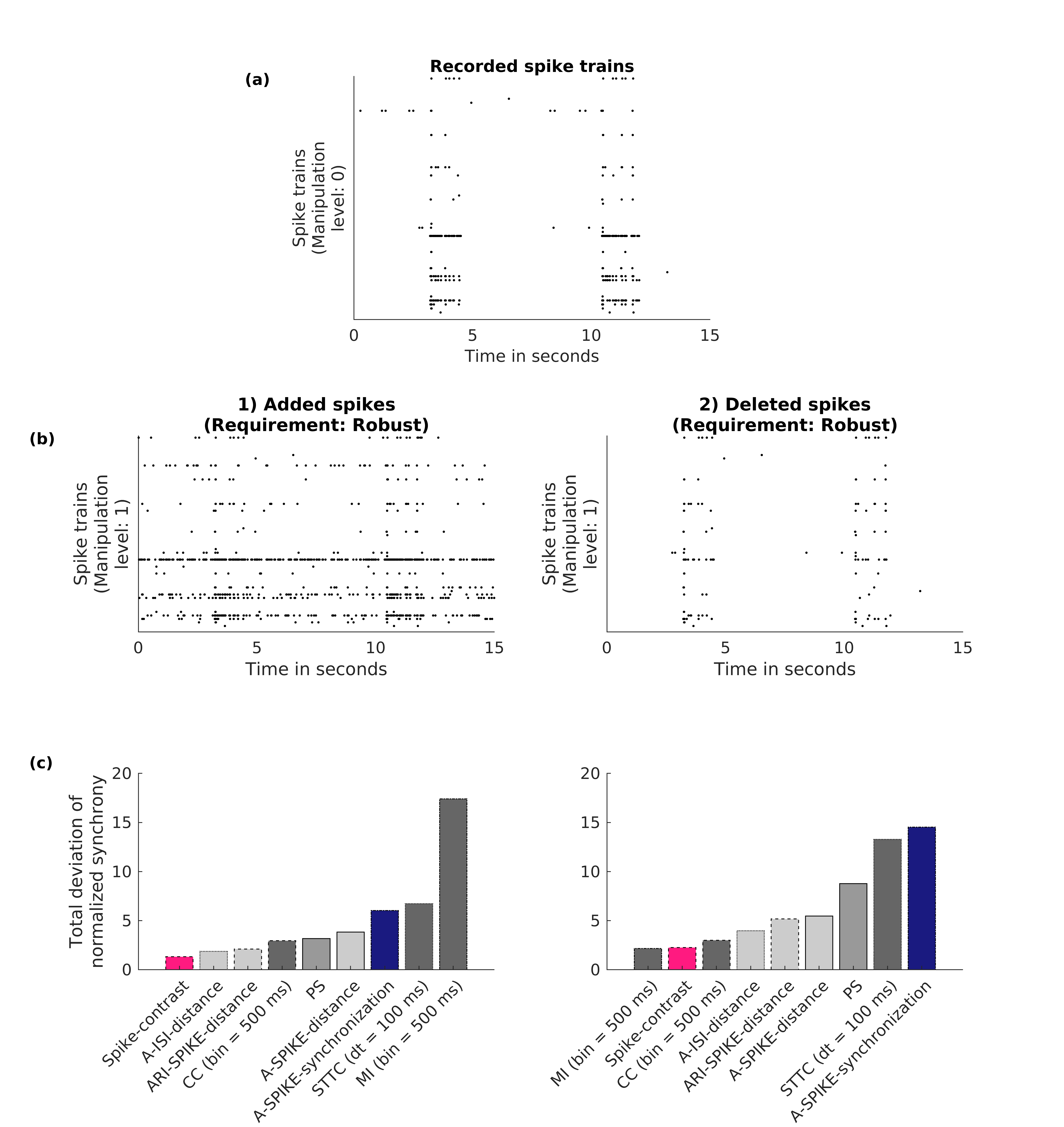
Figure 1: Comparison of different synchrony measures regarding their robustness to erroneous spike trains. (a) Spike trains recorded from 60 electrodes with 10 $\mu$M BIC. Each line represents the spike train of one electrode (only first 15 s of 300 s are displayed). (b) Same as (a) but with maximum manipulation level applied (left: Simulation of false positive spikes, right: Simulation of false negative spikes). In total 10 different recordings were used to generate the in silico manipulated data (for details see Sec. 2.2). (c) Sum of synchrony deviation over all manipulation levels (denoted as total deviation of the normalized synchrony (TDNS), see Eq. 5). The lower the TDNS value of a synchrony measure, the more robust it is to spike train manipulation.

2.3 Experimental data

2.1 Cell culture and electrophysiological recordings

Experimental data used for this study were recorded from primary cortical neurons (Lonza Ltd, Basel, Switzerland) harvested from embryonic rats (E18 and E19). Cell cultivation followed a modified protocol based on Otto et al. (2003). Briefly, vials containing 4$\times$10⁶ cells were stored in liquid nitrogen at -196⁰C. After thawing, cells were diluted drop-wise with pre-warmed cell culture medium and seeded at a density of 5000 cells/mm² onto Poly-D-Lysine and Laminin coated (Sigma Aldrich Co. LLC, St. Louis, USA) microelectrode arrays (60MEA200/30iR-Ti, Multichannel Systems MCS GmbH, Reutlingen, Germany). Twice a week, half of the medium was replaced with fresh, pre-warmed medium.
Neuronal signals were recorded extracellularly at a sampling rate of 10 kHz outside the incubator at 37⁰C employing a temperature-controller (Multichannel Systems MCS GmbH). For drug-induced increase of network synchronization, bicuculline (BIC) (Sigma Aldrich Co. LLC) was applied to the neuronal cell culture after 21  days in vitro (div) at a concentration of 10 $\mu$M. BIC is a competitive antagonist of the GABA_A receptor. Since it blocks the inhibitory function of GABA_A receptors, its application yields an increased incidence of synchronized burst events (Jungblut et al., 2009), see Fig. 2 (b) and (c). Neuronal activity was recorded for 5 minutes before and 5 minutes during the application of BIC.

2.2 Spike detection

Raw data were stored for offline spike detection with DrCell, a custom-made Matlab (MathWorks Inc., Natick, Massachusetts, U.S.A.) software tool, developed by Nick et al. (2013). After applying a high-pass filter with a cutoff frequency of 50 Hz, spikes were separated from noise using a threshold-based algorithm, with a threshold calculated by multiplying the standard deviation of the noise by a factor of 5 (or more precisely -5 as only negative spikes were used for analysis). As soon as the raw signal underran the threshold, the time of the minimum voltage value was defined as a spike time stamp (Fig. 2 (a)). Additionally, in order to alter the level of false positive and false negative spikes, spike detection was also conducted using threshold factors of 4, 6, and 7. For subsequent spike train analysis, only electrodes with more than 5 spikes per minute were considered active and used for analysis (Novellino et al., 2011).

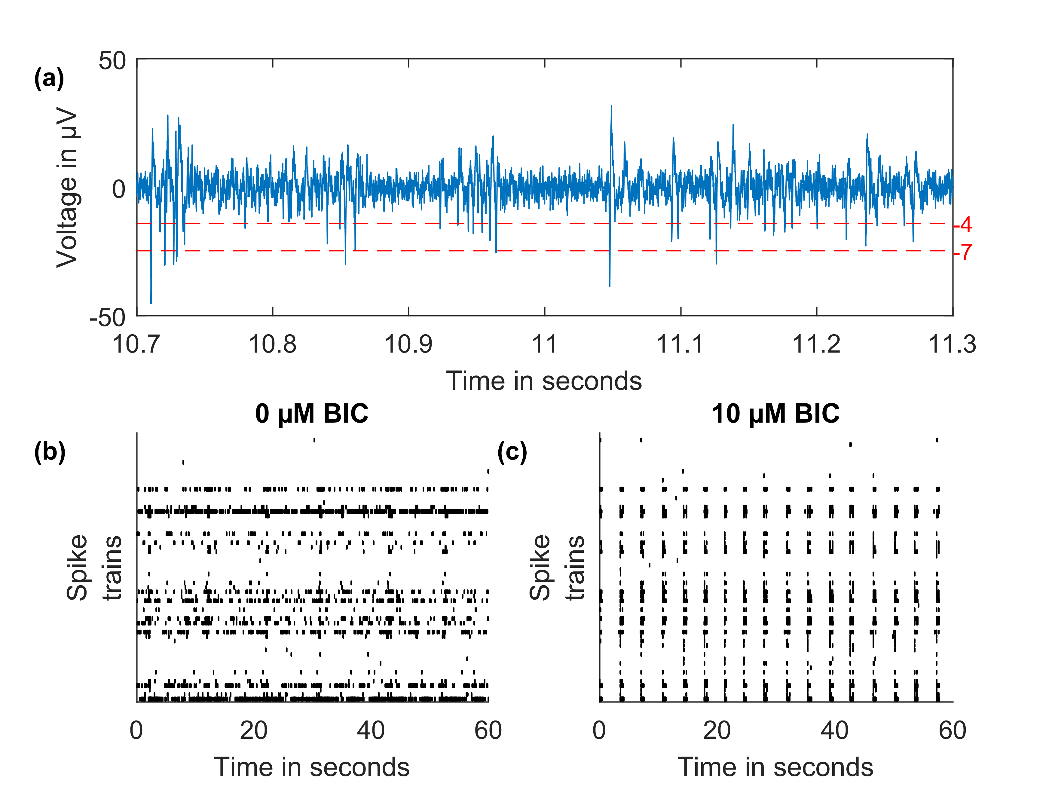
Figure 2: Exemplary illustration of the experimental data. (a) Signal recorded from one MEA electrode (50 Hz high-pass filtered). Thresholds are displayed for the lowest (4) and highest (7) threshold factors used for spike detection. The higher the threshold factor, the less spikes are detected. (b) Rasterplot of the spontaneous activity of one MEA chip without BIC (only first 60 s of 300 s are shown). (c) Same as (b) but with 10 $\mu$M BIC. Spontaneous activity was recorded with a 60 electrode MEA chip at 23 div. Compared to the native state, the administration of 10 $\mu$M BIC increased the level of synchrony.

2.3 Statistical analysis

Since it is known that BIC causes an increase of network synchrony in cortical neurons in vitro (Sokal et al., 2000; Chiappalone et al., 2007b; Eisenman et al., 2015), a one-tailed statistical test was applied. More specifically, a paired t-test was applied under the null hypothesis that BIC does not increase synchrony. The lower the p-value, the lower the probability that there is no synchrony change, and hence the better the synchrony measure’s sensitivity to BIC.

2.4 Parameter choice

As the synchrony measures CC, MI, and STTC depend on a time-scale parameter that directly influences the synchrony definition, an appropriate parameter value had to be chosen. Therefore, we analyzed the experimental BIC data using different parameter values and conducted a statistical hypothesis test. The lower the p-value, the higher the probability that an increase in synchrony occurred. Parameter values that lead to low p-values are therefore desirable (given that BIC results in increased level of synchrony). CC proposed by Selinger et al. (2004) chose a bin size of 500 ms, which also gave reasonable low p-values in our analysis (Fig. 3). Even if smaller bin sizes yielded lower p-values in our data, we stuck to the predefined 500 ms. For MI, we also chose a bin size of 500 ms as for smaller bin sizes the p-value only improved slightly. The parameter $dt$ of STTC was set to 100 ms according to the original publication from Cutts and Eglen (2014). Note that in our cortical data a larger dt value would only slightly improve the p-value.

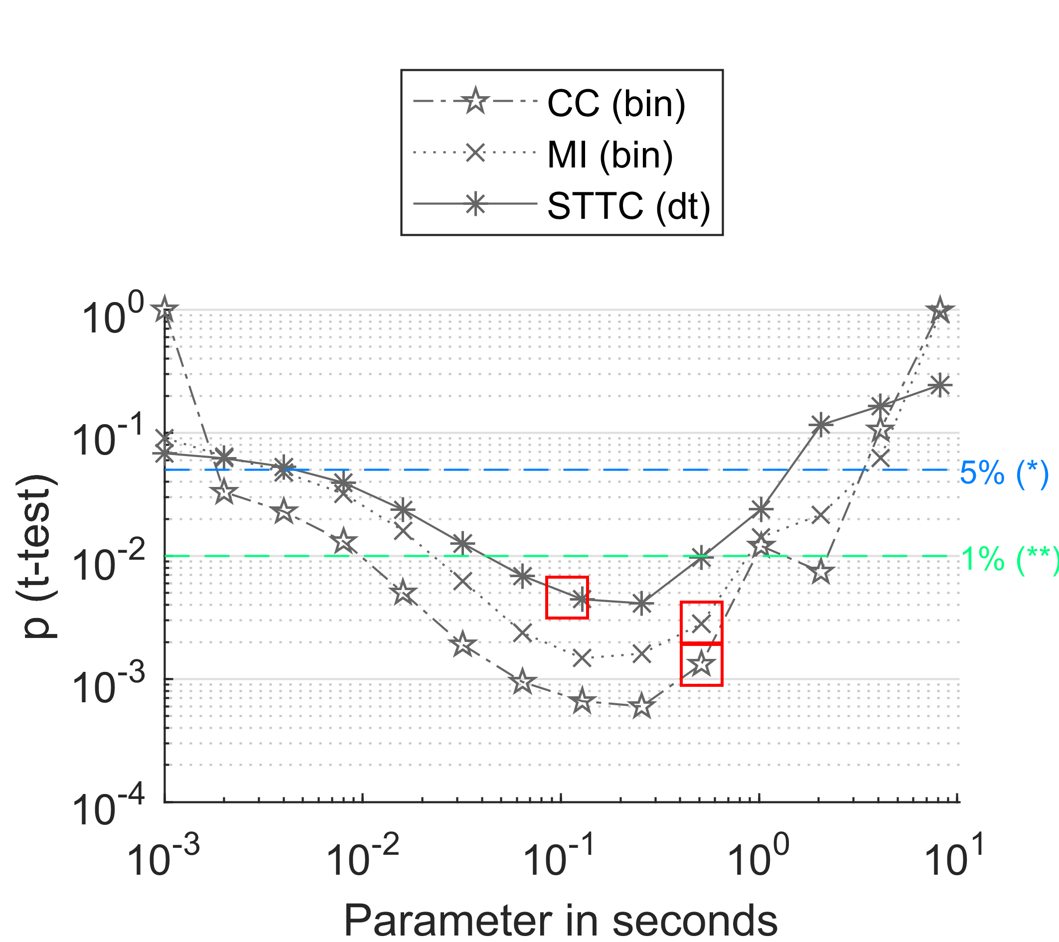
Figure 3: Influence of the parameter choice on the statistical significance of the experimental data. The synchrony measures CC, MI, and STTC depend on a parameter which has to be chosen by the user. For each synchrony measure, the experimental data described in Section 2.3 were analyzed using different parameter values. After that, a t-test was applied to the data with the null hypothesis that synchrony values of the data with BIC are lower or equal to synchrony values of the data without BIC. In this work, a bin size of 500 ms was used for CC and a $dt$ of 100 ms for STTC (red squares), as these values were suggested in their original publications. For MI, the same bin size as for CC was used due to the identical binning procedure.

3 Results

3.1 Comparison of synchrony measures for in silico manipulated data

• Added spikes: The robustness of measures was studied by randomly adding false positive spikes to the basic signals. For a robust synchrony measure low sensitivity to false positive spikes is desirable as such noise may falsify the results. As displayed in Fig. 1 (e 1) Spike-contrast was most robust to false positive spikes indicated by the small TDNS value of around $1$, closely followed by A-ISI-distance and ARI-SPIKE-distance. MI showed by far the largest synchrony deviation indicated by a TDNS value of around $17$.
  

• Deleted spikes: A similar picture occurs after increasingly deleting spikes in order to simulate false negative spikes, as robustness to false negative spikes was required. In Fig. 1 (e 2) results of synchrony measure dependency to false negative spikes are shown. Here, MI and Spike-contrast were most robust to false negative spikes yielding the smallest TDNS value of around $2$. STTC and A-SPIKE-synchronization showed largest TDNS value of around $14$.
  

3.2 Comparison of synchrony measures for experimental data

In addition to the evaluation with in silico manipulated data, all synchrony measures were applied to experimental data recorded from cortical neurons by MEA chips with and without the application of 10 $\mu$M BIC. Fig. 4 (a) shows the absolute synchrony values for each synchrony measure and for all different cell cultures ($N=5$), before and after the application of BIC. Generally all measures showed a significant synchrony increase due to the BIC application with p-values of 5% and below, where A-SPIKE-synchronization, A-ISI-distance, and A-SPIKE-distance failed to reach the high significance level of 1%.

In order to alter the level of false positive and false negative spikes in the experimental data, different spike detection threshold factors (4 to 7) were applied. Where low thresholds are likely to correspond to additional false spikes (false positive) and high thresholds to missed spikes (false negative). Increasing the threshold factor is comparable with deleting spikes from the spike train as already done in the in silico manipulated data evaluation (Section 3.1). For the in silico manipulated data, the synchrony measures STTC and A-SPIKE-synchronization were most sensitive to deleted spikes. This behavior was also evident within the experimental data (Fig. 5). As the spike detection threshold factor increased, STTC and A-Spike-synchronization lose their statistical significance (above 5% level), while all others remained stable indicating statistical significance (below 5% level). Spike-contrast yielded the highest statistical significance across all tested threshold factors, and was the only measures that still indicated a statistical significance (at 5% level) at the smallest threshold factor of 4, where a high level of noise spikes is assumable.

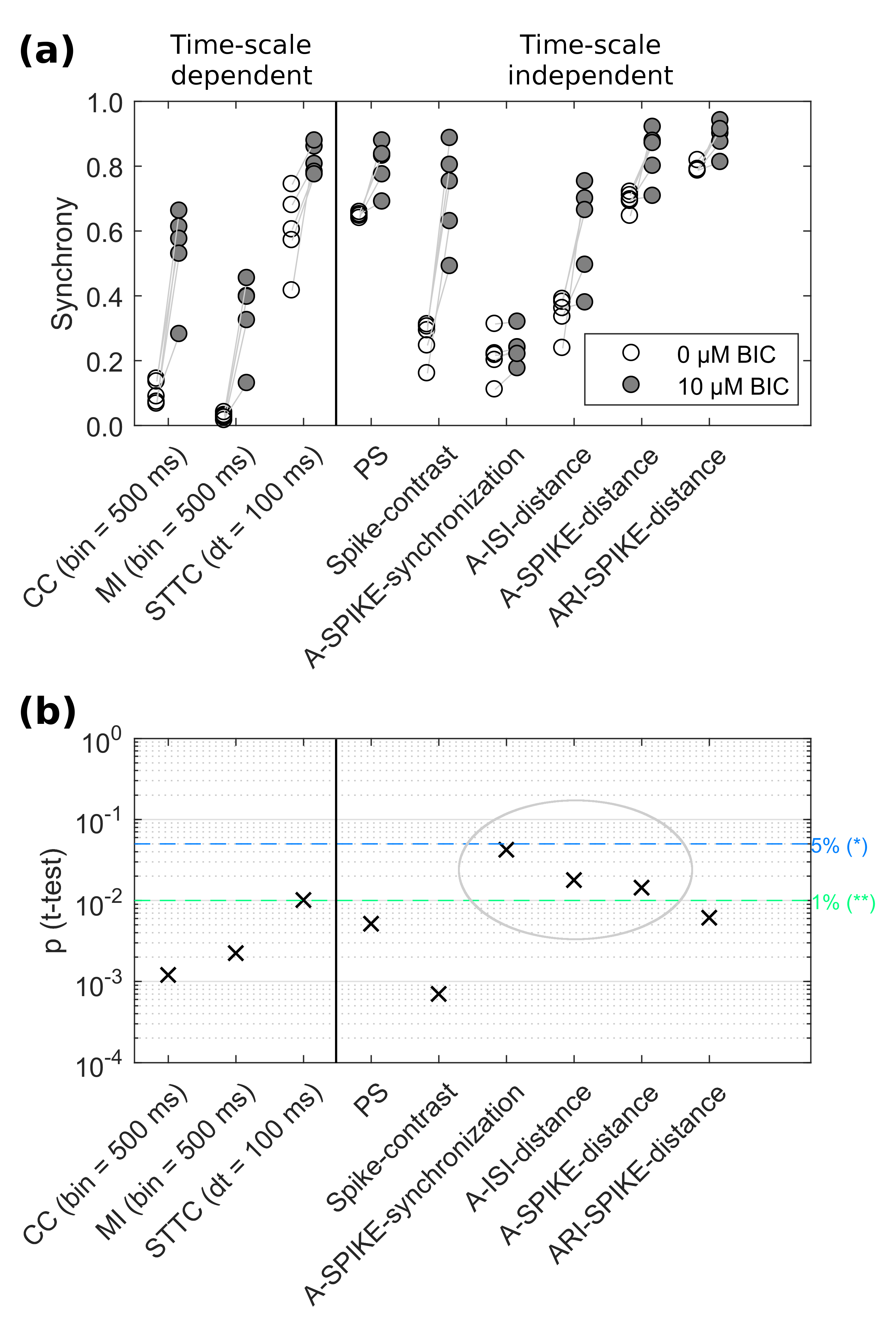
Figure 4: Results of the application of different time-scale dependent and time-scale independent synchrony measures to a set of experimental data. Experimental data were recorded from cortical cell cultures on MEA chips ($N=5$) in the absence and presence of 10 $\mu$M BIC. (a) Absolute synchrony values of each synchrony measure for data without BIC (white circles) and with BIC (gray circles). (b) P-values for each synchrony measure from a one-tailed paired t-test assuming an increase in synchrony. The lower the p-value, the better the synchrony measure’s ability to capture the effect of BIC. Grey ellipse marks synchrony measures that were not able to indicate high significant effects below p-values of 1%. Spike detection threshold factor was 5.

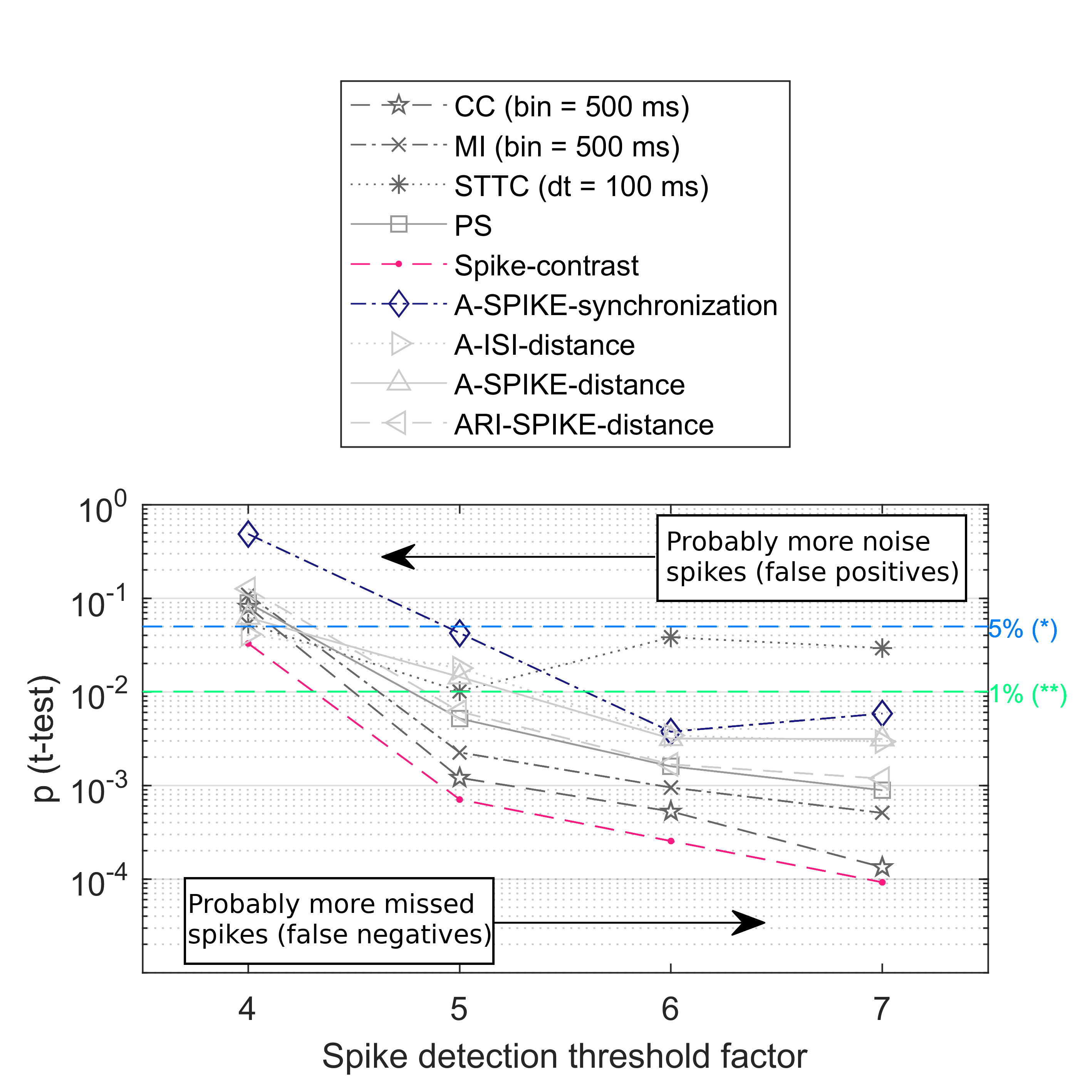
Figure 5: Influence of the spike detection threshold on the statistical significance of the experimental data. Synchrony and statistical significance of the experimental data were analyzed like in Fig. 4 applying different thresholds to detect spikes from the recorded signals. Assumably, the higher the spike detection threshold factor, the less noise were detected but also more real spikes were missed. The lower the p-value, the better the synchrony measure’s ability to capture the effect of BIC.

4 Discussion and Conclusion

In this work we compared different spike train synchrony measures regarding their robustness to false positive and false negative spikes in epileptiform signals. Such robustness is particularly relevant for experimental data with error prone spike detection, especially at low signal-to-noise ratios. Representative synchrony measures were chosen from different categories such as time-scale dependent (CC, MI, STTC), or time-scale independent (Spike-contrast, PS, A-SPIKE-synchronization, A-ISI-distance, A-SPIKE-distance, ARI-SPIKE-distance). In order to perform a comparison, we proposed a procedure based on a set of in silico manipulated spike trains with defined manipulation of features. Two data sets were generated based on experimental data by adding spikes, representing noise (false positive), and deleting spikes, representing missed spikes (false negative). Synchrony of the experimental data was increased by applying BIC to cortical in vitro networks. The code and data used in this work are publicly available (see Section 2.1).

For the in silico manipulated data, the results showed that Spike-contrast was most robust to added spikes and very robust to deleted spikes. All other measures showed either comparable high robustness for added or deleted spikes, but not for both cases. Furthermore, CC, MI, and Spike-contrast work with binnend spike trains, which explains their robustness to deleted spikes as long as bursts (=many spikes occuring within a small time period) are still present in the data (see Fig. 1, (b 2)). A binned spike train will almost not change if only some spikes are deleted from a burst and if the bin size and burst duration are similar. As Spike-contrast automatically adapts its bin-size to the data, it is preferable over CC and MI for exploratory studies, where the time-scale is not known beforehand.

For the experimental data, all synchrony measures captured the synchrony increase mediated by BIC in a statistical significant way (below a p-value of 5%). However, there were differences in performance as the synchrony measures CC, MI, PS, Spike-contrast, and ARI-SPIKE-distance yielded values leading to a high statistical significance below p-values of 1%. Note that for CC the proposed bin size of 500 ms was used, but smaller bin sizes of around 300 ms would have overperformed Spike-contrast (Fig. 3). Referring to our assumption “the lower the p-value, the better the synchrony measure” defined in Section 2.3, it must be taken into account that this assumption is controversial since the actual synchrony increase (=ground truth) is not known for the experimental data. Thus, a synchrony measure that overestimates the synchrony increase mediated by BIC would incorrectly lead to a low p-value.

For small sample sizes, as in our experiment ($N=5$), parameter-free statistics like the Wilcoxon signed-rank test are generally used to avoid assumptions about population distribution. Application of the Wilcoxon signed-rank test to our data yielded almost identical p-values for all synchrony measures (data not shown). In contrast, the t-test used in this work resulted in different p-values for each synchrony measure. So, it also depends on the choice of statistical test whether the choice of synchrony measures affects the final results.

Considering the results of the in silico manipulated data, the measures CC, MI, Spike-contrast, and ARI-SPIKE-distance were most robust to deleted spikes (=false negative spikes). As mentioned above, these synchrony measures also showed the best performance in the experimental data. This suggests that robustness to false negative spikes correlates with the ability to quantify synchrony changes in experimental data. If so, it would also imply that the experimental data used in this work were more affected by false negative spikes, than by false positive spikes. In other words, more spikes were missed than noise was misinterpreted as spikes. This behavior could be used to draw conclusions about the quality of an experimental spike train from the rank of the p-values of different synchrony measures.

Like already mentioned, there were some synchrony measures, whose results of the in silico manipulated data and experimental data did not correlate. This suggests, that robustness to false positive or false negative spikes is not the only factor to effectively capture synchrony changes in experimental data. Factors like robustness to temporal non-stationarity of the recording could also be different among the synchrony measures. For instance, PS, A-SPIKE-distance, ARI-SPIKE-distance, A-ISI-distance, and A-SPIKE-synchronization are more adaptive to changes in time scales inside a spike train as they dynamically define their time scales considering nearby spikes. In contrast, CC, MI, STTC, and Spike-contrast use equally spaced time scales along the entire spike train duration.

Overall, for our specific data set, Spike-contrast was the only time-scale independent measure being robust to noise (false positive spikes) as well as missed spikes (false negative spikes). This desirable performance was confirmed by the ability of the Spike-contrast measure to detect biochemically induced synchrony with a high significance, even for different spike detection threshold factors. It should be mentioned that the measures A-SPIKE-synchronization, A-ISI-distance, A-SPIKE-distance, and ARI-SPIKE-distance are able to produce a synchrony profile over time, which complements the synchrony profile over time-scale of Spike-contrast.

Summarizing, we suggest to include the Spike-contrast synchrony measure into synchrony studies of epileptiform experimental neuronal data sets in addition to established synchrony measures.

4.1 Acknowledgments

F.A.R. acknowledge CNPq (grant 305940/2010-4), Fapesp (grant 2012/51301-8 and 2013/26416-9) and NAP eScience - PRP - USP for financial support. L.F.C. thanks CNPq (grant 307085/2018-0) and FAPESP (grant 15/22308-2) for sponsorship. G.F.A. acknowledges FAPESP (grant 2012/25219-2). T.P. acknowledges FAPESP (grant 2016/23827-6). C.C.H. acknowledges FAPESP (grant 18/09125-4). C.T. and M.C. acknowledges Bayerisches Staatsministerium für Bildung und Kultus, Wissenschaft und Kunst for financial support in the frame of ZEWIS, BAYLAT, the BMBF (grant 03FH061PX3), and INeuTox (grant 13FH516IX6). C.N. would like to acknowledge support from the Studienstiftung des Deutschen Volkes.

5 Appendix

5.1 Synchrony measure description

Mutual Information

MI measures how two random variables $X$ and $Y$ are related (Cover and Thomas, 2012) and is based on the concept of entropy, which is a fundamental concept in information theory (Shannon and Weaver, 1948; Cover and Thomas, 2012). The Shannon entropy (Cover and Thomas, 2012) of a random variable $X$ is defined as

$$H(X)=-\sum_{i}p_{x}(i)\log(p_{x}(i)),$$ (6)

where $p_{x}(i)=P(X=i)$ and the $\log$ function is taken to the base $2$ (see Fig. 6 a for an example calculation). $H(X)$ measures the uncertainty about a random variable $X$. The conditional entropy quantifies the information necessary to describe the random variable $Y$ given that the information about $X$ is known (Cover and Thomas, 2012). Formally, it is defined by

$$H(Y|X) \equiv\sum_{x\in X}\,p(x)\,H(Y|X=x)$$ (7)

$${=}\sum_{x\in X}\left(p(x)\sum_{y\in Y}\,p(y|x)\,\log\,\frac{1}{p(y|x)}\right)$$

$$=-\sum_{x\in X}\sum_{y\in Y}\,p(x,y)\,\log\,p(y|x)$$

$$=-\sum_{x\in X,y\in Y}p(x,y)\log\,p(y|x)$$

$$=\sum_{x\in X,y\in Y}p(x,y)\log\frac{p(x)}{p(x,y)}.$$

MI is defined as

$$I(X;Y)=\sum_{y\in Y}\sum_{x\in X}p(x,y)\log{\left(\frac{p(x,y)}{p(x)\,p(y)}\right)}.$$ (8)

Additionally, the MI can be expressed in terms of the entropy and the conditional entropy of random variables $X$ and $Y$ as

$$I(X;Y) {}=H(X)-H(X|Y)$$ (9)

$${}=H(Y)-H(Y|X)$$

$${}=H(X)+H(Y)-H(X,Y)$$

$${}=H(X,Y)-H(X|Y)-H(Y|X).$$

Aside from the analytic expressions, it is possible to interpret those quantities graphically, as depicted in Fig. 6b. MI is more general than the correlation coefficient and quantifies how the joint distribution $p(x,y)$ is similar to the products of marginal distributions $p(x)p(y)$ (Cover and Thomas, 2012). Compared to the cross-correlation measure, mutual information also captures non-linear dependencies.

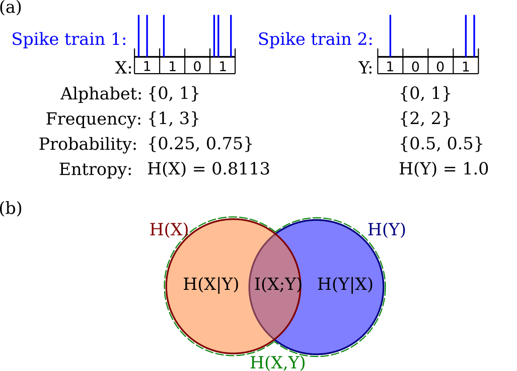
Figure 6: Example entropy calculation of two spike trains and illustration of the mutual information (MI) measure. (a) Two different spike trains are binned in a binary way resulting in X and Y. Each value is considered a character building the alphabet of the signal. The probability of each character is obtained by dividing its incidence by the length of the signal. The entropy of each signal (H(X), H(Y)) is calculated using Eq. (6) with the probabilities given above. (b) Visualization of the mutual information I(X;Y) using the joint entropy H(X,Y), the entropies H(X), H(Y), and conditional entropies H(X$|$Y), H(Y$|$X) like calculated in Eq. (9). The mutual information value I(X;Y) increases with increasing synchrony between signal X and Y.

For comparison, the value of mutual information needs to be normalized. Many possible approaches have been proposed (Cover and Thomas, 2012), such as

$$M(X;Y)=\frac{I(X;Y)}{\min\left[H(X),H(Y)\right]},$$ (10)

because $I(X;Y)\leq\min\left[H(X),H(Y)\right]$ and, consequently, $0\leq M(X;Y)\leq 1$. This formulation has been used before in the context of neuronal signal analysis (Bettencourt et al., 2007, 2008; Ham et al., 2010). Another possible normalization is the so-called symmetric uncertainty (Witten and Frank, 2000), defined as

$$M^{*}(X;Y)=2\frac{I(X;Y)}{H(X)+H(Y)},$$ (11)

where $0\leq M^{*}(X;Y)\leq 1$. In this work the latter normalization were used as it performed better than the first one when applied to the experimental data (data not shown).

In order to estimate the MI between two spike trains, both spike trains were transformed into binary binned signals. A spike train $i$ is binnend as

$$x_{i}(t)=\begin{cases}\text{$1$, if spike train $i$ shows at least one spike in time interval $t$ to $t+\Delta t$.}\\ \text{$0$, if spike train $i$ shows no spike in time interval $t$ to $t+\Delta t$.}\end{cases}$$ (12)

using a bin size $\Delta t=$ 500 ms and $t=0\Delta t,1\Delta t,2\Delta t,...$ (also see Fig. 6 a). The choice of the bin size of 500 ms is justified in Section 2.4).

Phase Synchronization

Since synchronization processes are related with rhythm adjustment, it is natural to introduce the concept of phase of an oscillator, a quantity that increases by $2\pi$ within an oscillation cycle and determines unambiguously the state of a periodic oscillator (Pikovsky et al., 2003). For instance, consider a harmonic oscillator described by the variable $x(t)=A\sin(\omega_{0}t+\phi_{0})$. In this case, $\omega_{0}$ denotes the angular frequency, which is related to the oscillation period $\omega_{0}=2\pi/T$, $A$ is the amplitude of oscillation, and the quantity $\phi(t)=\omega_{0}t+\phi_{0}$ is the phase of this oscillator. Two or more oscillators are synchronized when they present the same phase evolution (Pikovsky et al., 2003).

The measurement of the synchronization level of self-sustained oscillators can be done by considering the phases as rotating points in the unit cycle of the complex plane (Pikovsky et al., 2003; Strogatz, 2000). If an oscillator has a phase $\phi(t)$, then its trajectory in the complex plane is described by the vector $e^{i\phi(t)}$. For instance, if two oscillators have phases $\phi_{1}(t)=\phi_{2}(t)=\phi(t)$, then they will have the same trajectory in the complex plane and thus the modulus of the resultant vector will be $|e^{i\phi_{1}(t)}+e^{i\phi_{2}(t)}|/2=1$, meaning that the oscillators are perfectly synchronized. Supposing now a population of $N$ interacting phase oscillators whose phases are described by the variable $\phi_{i}(t)$, $i=1,...,N$. The synchronization order parameter is defined as (Strogatz, 2000)

$$re^{i\psi(t)}=\frac{1}{N}\sum_{j=1}^{N}e^{i\phi_{j}(t)},$$ (13)

where $\psi(t)$ is the average phase of the system at time $t$. When $r\approx 0$, the phases are distributed uniformly over $[0,2\pi]$ corresponding to the asynchronous state. When $r\approx 1$ the phases rotate together corresponding to fully synchronized state (Fig. 7).

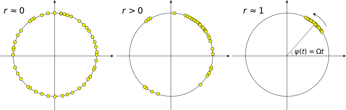
Figure 7: Example for distribution of phase vectors $e^{i\phi(t)}$ in complex plane. (a) Randomly distributed phase vectors over $[0,2\pi]$, implying $r\approx 0$; in other words the oscillators are completely asynchronous. (b) Regime of partial synchronization; phase vectors of some oscillators are grouped in a synchronous cluster equivalent to $r>0$. (c) Strongly synchronized state, where all oscillators group into a single synchronous cluster rotating with average frequency $\Omega$, thus $r\approx 1$.

Neurons can also be considered as self-sustained oscillators (Arenas et al., 2008) and are often modeled as integrate-and-fire oscillators, where the rhythmic quantity is the rate at which spikes are fired. The synchronization process in this case is the adjustment of the spiking patterns, i.e., if two interacting integrate-and-fire oscillators discharge their spikes jointly, then they are synchronized. Therefore, in order to quantify the synchronization between interacting integrate-and-fire oscillators, the phases associated to the respective spike signals have to be defined.

The time series recorded by an electrode can be considered as a sequence of point events taking place at time $t_{k}$, with $k=1,2,...,N_{\mathrm{spikes}}$. The time interval between two spikes can be treated as a complete cycle. In this case, the phase increase during this time interval is exactly $2\pi$. Hence, the values of $\phi(t_{k})=2\pi k$ are assigned to the times $t_{k}$, and for an arbitrary instant of time ($t_{k}<t<t_{k+1}$), the phase is considered as a linear interpolation between these values (Pikovsky et al., 2003; Neiman et al., 1998; Pikovsky et al., 1997; Tass et al., 1998; Hu and Zhou, 2000), as

$$\phi(t)=2\pi\frac{t-\tau_{k}}{\tau_{k+1}-\tau_{k}}+2\pi k.$$ (14)

This method can be applied to any process containing time series of spikes and it is widely used in the study of synchronization in neuronal dynamics (Pikovsky et al., 2003). Fig. 8 exemplifies the calculation of phases $\phi(t)$ of two spike signals and their respective sum of the phase vectors $e^{i\phi(t)}$ in the complex plane.

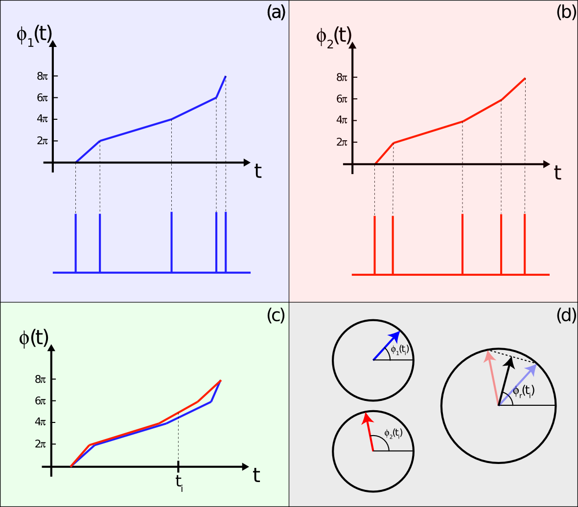
Figure 8: Example of phase vector construction. (a) $\phi_{1}(t)$ and (b) $\phi_{2}(t)$ are calculated using the respective spike signals according to Equation (14). (c) Superposition of temporal evolution of phases and (d) phase vectors $e^{i\phi_{1}(t_{i})}$, $e^{i\phi_{2}(t_{i})}$ as well as the resultant vector at time $t=t_{i}$, $r\cdot e^{i\phi_{r}(t_{i})}=(e^{i\phi_{1}(t_{i})}+e^{i\phi_{2}(t_{i})})/2$.

For a system composed of $N$ oscillators, the instant phase synchronization is quantified by the order parameter defined in Eq. (13). However, to quantify the level of synchronization of the neurons, we consider the average over the recorded time

$$\bar{r}=\left\langle\left|\frac{1}{N}\sum_{j=1}^{N}e^{i\phi_{j}(t)}\right|\right\rangle_{t},$$ (15)

where $\left\langle\cdots\right\rangle_{t}$ stands for the temporal average and $N$ stands for the number of electrodes used to compute the order parameter.

6 Author contributions

M.C.: Conception, design, generation, and analysis of in silico manipulated data. Application of the synchrony measures STTC, Spike-contrast, A-SPIKE-synchronization, A-ISI-distance, A-SPIKE-distance, ARI-SPIKE-distance to experimental data. Statistical tests and spike detection with varying thresholds. Preparation of figure 1 to 6. Draft of the manuscript. R.B.: Initial conception and design of synchrony measure comparison using experimental data. C.N.: Initial conception and design of synchrony measure comparison using experimental data. Performed cell experiments and spike detection of raw data. G.F.A.: Implementation and application of the synchrony measure MI to experimental data and MI description in appendix. T.P.: Implementation and application of the synchrony measure PS to experimental data and PS description in appendix. Preparation of figure 7 and 8. C.C.H.: Implementation and application of the synchrony measures CC to experimental data. L.F.C.: Helped in the initial conception, discussions and revision. F.A.R.: Conception and design of research. C.T.: Conception and design of research. ALL: Interpreted and discussed results of experiments. Edited and revised manuscript. Approved final version of manuscript.

References

- Andrzejak et al. (2014) Andrzejak, R. G., Mormann, F., Kreuz, T., 2014. Detecting determinism from point processes. Physical Review E 90 (6), 062906.
- Arenas et al. (2008) Arenas, A., Díaz-Guilera, A., Kurths, J., Moreno, Y., Zhou, C., 2008. Synchronization in complex networks. Physics Reports 469 (3), 93–153.
- Arnulfo et al. (2015) Arnulfo, G., Canessa, A., Steigerwald, F., Pozzi, N. G., Volkmann, J., Massobrio, P., Martinoia, S., Isaias, I. U., 2015. Characterization of the spiking and bursting activity of the subthalamic nucleus in patients with parkinson’s disease. In: Advances in Biomedical Engineering (ICABME), 2015 International Conference on. IEEE, pp. 107–110.
- Bettencourt et al. (2007) Bettencourt, L., Stephens, G., Ham, M., Gross, G., Feb. 2007. Functional structure of cortical neuronal networks grown in vitro. Physical Review E 75 (2), 021915.
- Bettencourt et al. (2008) Bettencourt, L. M. A., Gintautas, V., Ham, M. I., Jun 2008. Identification of Functional Information Subgraphs in Complex Networks. Phys. Rev. Lett. 100, 238701.
- Chiappalone et al. (2006) Chiappalone, M., Bove, M., Vato, A., Tedesco, M., Martinoia, S., 2006. Dissociated cortical networks show spontaneously correlated activity patterns during in vitro development. Brain research 1093 (1), 41–53.
- Chiappalone et al. (2007a) Chiappalone, M., Vato, A., Berdondini, L., Koudelka-Hep, M., Martinoia, S., 2007a. Network dynamics and synchronous activity in cultured cortical neurons. International Journal of Neural Systems 17 (02), 87–103.
- Chiappalone et al. (2007b) Chiappalone, M., Vato, A., Berdondini, L., Koudelka-Hep, M., Martinoia, S., 2007b. Network dynamics and synchronous activity in cultured cortical neurons. International Journal of Neural Systems 17 (02), 87–103.
- Ciba et al. (2018) Ciba, M., Isomura, T., Jimbo, Y., Bahmer, A., Thielemann, C., 2018. Spike-contrast: A novel time scale independent and multivariate measure of spike train synchrony. Journal of Neuroscience Methods 293 (Supplement C), 136 – 143.
- Cover and Thomas (2012) Cover, T. M., Thomas, J. A., 2012. Elements of information theory. John Wiley & Sons.
- Cutts and Eglen (2014) Cutts, C. S., Eglen, S. J., 2014. Detecting pairwise correlations in spike trains: an objective comparison of methods and application to the study of retinal waves. The Journal of Neuroscience 34 (43), 14288–14303.
- Dura-Bernal et al. (2016) Dura-Bernal, S., Li, K., Neymotin, S. A., Francis, J. T., Principe, J. C., Lytton, W. W., 2016. Restoring behavior via inverse neurocontroller in a lesioned cortical spiking model driving a virtual arm. Frontiers in Neuroscience 10.
- Eisenman et al. (2015) Eisenman, L. N., Emnett, C. M., Mohan, J., Zorumski, C. F., Mennerick, S., 2015. Quantification of bursting and synchrony in cultured hippocampal neurons. Journal of Neurophysiology 114 (2), 1059–1071.
- Engel et al. (2001) Engel, A. K., Fries, P., Singer, W., 2001. Dynamic predictions: oscillations and synchrony in top–down processing. Nature Reviews Neuroscience 2 (10), 704–716.
- Espinal et al. (2016) Espinal, A., Rostro-Gonzalez, H., Carpio, M., Guerra-Hernandez, E. I., Ornelas-Rodriguez, M., Puga-Soberanes, H., Sotelo-Figueroa, M. A., Melin, P., 2016. Quadrupedal robot locomotion: a biologically inspired approach and its hardware implementation. Computational Intelligence and Neuroscience 2016.
- Fisher et al. (2005) Fisher, R. S., Boas, W. v. E., Blume, W., Elger, C., Genton, P., Lee, P., Engel, J., 2005. Epileptic seizures and epilepsy: definitions proposed by the international league against epilepsy (ilae) and the international bureau for epilepsy (ibe). Epilepsia 46 (4), 470–472.
- Flachs and Ciba (2016) Flachs, D., Ciba, M., 2016. Cell-based sensor chip for neurotoxicity measurements in drinking water. Lékař a technika - Clinician and Technology 46 (2), 46–50.
- Ham et al. (2010) Ham, M. I., Gintautas, V., Rodriguez, M. a., Bennett, R. a., Maria, C. L. S., Bettencourt, L. M. a., Jan. 2010. Density-dependence of functional development in spiking cortical networks grown in vitro. Biological cybernetics 102 (1), 71–80.
- Hu and Zhou (2000) Hu, B., Zhou, C., Feb 2000. Phase synchronization in coupled nonidentical excitable systems and array-enhanced coherence resonance. Phys. Rev. E 61, R1001–R1004.
- Jungblut et al. (2009) Jungblut, M., Knoll, W., Thielemann, C., Pottek, M., 2009. Triangular neuronal networks on microelectrode arrays: an approach to improve the properties of low-density networks for extracellular recording. Biomedical microdevices 11 (6), 1269–1278.
- Kreuz et al. (2011) Kreuz, T., Chicharro, D., Greschner, M., Andrzejak, R. G., 2011. Time-resolved and time-scale adaptive measures of spike train synchrony. Journal of Neuroscience Methods 195 (1), 92–106.
- Kreuz et al. (2013) Kreuz, T., Chicharro, D., Houghton, C., Andrzejak, R. G., Mormann, F., 2013. Monitoring spike train synchrony. Journal of Neurophysiology 109 (5), 1457–1472.
- Kreuz et al. (2007) Kreuz, T., Haas, J. S., Morelli, A., Abarbanel, H. D., Politi, A., 2007. Measuring spike train synchrony. Journal of Neuroscience Methods 165 (1), 151–161.
- Kreuz et al. (2015) Kreuz, T., Mulansky, M., Bozanic, N., 2015. Spiky: A graphical user interface for monitoring spike train synchrony. Journal of Neurophysiology 113 (9), 3432–3445.
- Li et al. (2011) Li, W., Doyon, W. M., Dani, J. A., 2011. Acute in vivo nicotine administration enhances synchrony among dopamine neurons. Biochemical pharmacology 82 (8), 977–983.
- Lieb et al. (2017) Lieb, F., Stark, H.-G., Thielemann, C., 2017. A stationary wavelet transform and a time-frequency based spike detection algorithm for extracellular recorded data. Journal of neural engineering 14 (3), 036013.
- Neiman et al. (1998) Neiman, A., Silchenko, A., Anishchenko, V., Schimansky-Geier, L., Dec 1998. Stochastic resonance: Noise-enhanced phase coherence. Phys. Rev. E 58, 7118–7125.
- Nick et al. (2013) Nick, C., Goldhammer, M., Bestel, R., Steger, F., Daus, A., Thielemann, C., 2013. Drcell—a software tool for the analysis of cell signals recorded with extracellular microelectrodes. Signal Processing: An International Journal (SPIJ) 7, 96–109.
- Novellino et al. (2011) Novellino, A., Scelfo, B., Palosaari, T., Price, A., Sobanski, T., Shafer, T. J., Johnstone, A. F., Gross, G. W., Gramowski, A., Schroeder, O., et al., 2011. Development of micro-electrode array based tests for neurotoxicity: assessment of interlaboratory reproducibility with neuroactive chemicals. Frontiers in neuroengineering 4.
- Otto et al. (2003) Otto, F., Goertz, P., Fleischer, W., Siebler, M., 2003. Cryopreserved rat cortical cells develop functional neuronal networks on microelectrode arrays. Journal of Neuroscience Methods 128, 173.
- Pare et al. (1990) Pare, D., Curro’Dossi, R., Steriade, M., 1990. Neuronal basis of the parkinsonian resting tremor: a hypothesis and its implications for treatment. Neuroscience 35 (2), 217–226.
- Pikovsky et al. (2003) Pikovsky, A., Rosenblum, M., Kurths, J., 2003. Synchronization: A universal concept in nonlinear sciences. Vol. 12. Cambridge University Press.
- Pikovsky et al. (1997) Pikovsky, A. S., Rosenblum, M. G., Osipov, G. V., Kurths, J., 1997. Phase synchronization of chaotic oscillators by external driving. Physica D: Nonlinear Phenomena 104 (3), 219–238.
- Rosenbaum et al. (2014) Rosenbaum, R., Tchumatchenko, T., Moreno-Bote, R., 2014. Correlated neuronal activity and its relationship to coding, dynamics and network architecture. Frontiers in computational neuroscience 8, 102.
- Satuvuori et al. (2017) Satuvuori, E., Mulansky, M., Bozanic, N., Malvestio, I., Zeldenrust, F., Lenk, K., Kreuz, T., 2017. Measures of spike train synchrony for data with multiple time scales. Journal of Neuroscience Methods.
- Selinger et al. (2004) Selinger, J. V., Pancrazio, J. J., Gross, G. W., 2004. Measuring synchronization in neuronal networks for biosensor applications. Biosensors and Bioelectronics 19 (7), 675–683.
- Shannon and Weaver (1948) Shannon, C., Weaver, W., 1948. A mathematical theory of communication. Bell Syst. Tech. J 27 (379), 623.
- Sokal et al. (2000) Sokal, D. M., Mason, R., Parker, T. L., 2000. Multi-neuronal recordings reveal a differential effect of thapsigargin on bicuculline-or gabazine-induced epileptiform excitability in rat hippocampal neuronal networks. Neuropharmacology 39 (12), 2408–2417.
- Strogatz (2000) Strogatz, S., 2000. From Kuramoto to Crawford: exploring the onset of synchronization in populations of coupled oscillators. Physica D: Nonlinear Phenomena 143 (1), 1–20.
- Tass et al. (1998) Tass, P., Rosenblum, M. G., Weule, J., Kurths, J., Pikovsky, A., Volkmann, J., Schnitzler, A., Freund, H.-J., Oct 1998. Detection of : Phase Locking from Noisy Data: Application to Magnetoencephalography. Phys. Rev. Lett. 81, 3291–3294.
- Truccolo et al. (2014) Truccolo, W., Ahmed, O. J., Harrison, M. T., Eskandar, E. N., Cosgrove, G. R., Madsen, J. R., Blum, A. S., Potter, N. S., Hochberg, L. R., Cash, S. S., 2014. Neuronal ensemble synchrony during human focal seizures. Journal of Neuroscience 34 (30), 9927–9944.
- Ward (2003) Ward, L. M., 2003. Synchronous neural oscillations and cognitive processes. Trends in Cognitive Sciences 7 (12), 553–559.
- Witten and Frank (2000) Witten, I., Frank, E., 2000. Data Mining. Practical Machine Learning Tools and Techniques with Java Implementations. Morgan Kaufmann.
- Wong et al. (1993) Wong, R. O., Meister, M., Shatz, C. J., 1993. Transient period of correlated bursting activity during development of the mammalian retina. Neuron 11 (5), 923–938.