Nonperturbative Dyson-Schwinger equation approach to strongly interacting Dirac fermion systems

Abstract

Studying the strong correlation effects in interacting Dirac fermion systems is one of the most challenging problems in modern condensed matter physics. The long-range Coulomb interaction and the fermion-phonon interaction can lead to a variety of intriguing properties. In the strong-coupling regime, weak-coupling perturbation theory breaks down. The validity of $1/N$ expansion with $N$ being the fermion flavor is also in doubt since $N$ equals to $2$ or $4$ in realistic systems. Here, we investigate the interaction between (1+2)- and (1+3)-dimensional massless Dirac fermions and a generic scalar boson, and develop an efficient non-perturbative approach to access the strong-coupling regime. We first derive a number of self-consistently coupled Ward-Takahashi identities based on a careful symmetry analysis and then use these identities to show that the full fermion-boson vertex function is solely determined by the full fermion propagator. Making use of this result, we rigorously prove that the full fermion propagator satisfies an exact and self-closed Dyson-Schwinger integral equation, which can be solved by employing numerical methods. A major advantage of our non-perturbative approach is that there is no need to employ any small expansion parameter. Our approach provides a unified theoretical framework for studying strong Coulomb and fermion-phonon interactions. It may also be used to approximately handle the Yukawa coupling between fermions and order-parameter fluctuations around continuous quantum critical points. Our approach is applied to treat the Coulomb interaction in undoped graphene. We find that the renormalized fermion velocity exhibits a logarithmic momentum-dependence but is nearly energy independent, and that no excitonic gap is generated by the Coulomb interaction. These theoretical results are consistent with experiments in graphene.

I Introduction

Developing efficient theoretical and numerical methods to handle the strong interactions of quantum many-body systems is absolutely one of the most challenging problems of condensed matter physics. In ordinary Fermi liquid systems, weak repulsive interaction is known to be irrelevant at low energies. This ensures that the conventional method of weak-coupling perturbative expansion is applicable AGD ; ColemanBook . Using perturbation theory, one can expand a physical quantity as the sum of an infinite number of terms, each of which is proportional to certain power of a small coupling constant $\lambda$. Usually one only needs to compute the leading one or two terms since the contributions of all the sub-leading terms are supposed to be negligible. Apparently, the perturbation theory is valid only when $\lambda$ is sufficiently small. It is broadly recognized that the inter-particle interaction is strong in many condensed matter systems, such as cuprate superconductors Lee06 , heavy fermion compounds Heavy , and certain types of Dirac/Weyl semimetals CastroNeto ; Kotov12 ; Vafek14 ; Wehling14 ; Armitage17 ; Tang18 . In these materials, strong interactions may lead to a variety of non-Fermi liquid (NFL) behaviors and quantum phase transitions. When the coupling parameter $\lambda$ is at the order of unity or much larger than unity, the traditional method of perturbative expansion breaks down and can no longer be trusted.

In order to study strong inter-particle interactions, it is necessary to go beyond the framework of weak-coupling perturbative expansion. A frequently used method is to generalize the fermion flavor $N$ to a large number and expand physical quantities in powers of $1/N$. As $N\rightarrow\infty$, one might be able to consider only the leading one or two terms, based on the expectation that all the higher order contributions are suppressed. This expansion scheme has been previously applied to investigate strongly correlated electronic systems Polchinski94 ; Altshuler94 ; Kim94 ; Kim97 ; Rantner01 ; Rech06 ; Kim08 ; Metlitski20101 ; Metlitski20102 ; Raghu19 . However, the main problem of this approach is that in most realistic systems the physical value of fermion flavor is $N=2$, corresponding to spin degeneracy. It is unclear whether the results obtained in the $N\rightarrow\infty$ limit are still reliable as $N$ is reduced down to its physical value. Actually, the $1/N$ expansion scheme may be invalid even in the $N\rightarrow\infty$ limit. As argued by Lee Lee09 , the leading contribution of $1/N$ expansion contains an infinite number of Feynman diagrams as $N\rightarrow\infty$ in the U(1) gauge model of spin liquids.

Over the last 15 years, Dirac semimetal materials CastroNeto ; Kotov12 ; Vafek14 ; Wehling14 ; Armitage17 ; Tang18 have been extensively studied. Such materials do not have a finite Fermi surface, and the conduction and valence bands touch at discrete points, around which relativistic Dirac fermions emerge as low-lying elementary excitations. Graphene Geim05 ; Geim07 and surface state of three-dimensional topological insulator Vafek14 ; Wehling14 ; Armitage17 ; Hasan10 ; Qi11 are two typical $(1+2)$-dimensional Dirac semimetals. $(1+3)$-dimensional Dirac semimetal may be realized in TiBiSe_2-xS_x XuSuYang11 ; Sato11 , Bi_2-xIn_xSe₃ Brahlek12 ; Wu13 , and also Na₃Bi and Cd₃As₂ Wangzj12 ; Wangzj13 ; LiuZK14A ; Neupane14 ; LiuZK14B ; Borisenko14 ; HeLP14 ; ZhangFaXianXiu19 . Dirac fermions exhibit different properties from the Schrodinger electrons excited around the finite Fermi surface of a normal metal. The unique electronic structures of Dirac semimetals lead to prominent new features. The first new feature is that, Dirac fermions have more degrees of freedom than Schrodinger electrons. The latter only have two spin components, thus the unity matrix (in spin-independent cases) and the Pauli matrices (in spin-dependent cases) suffice to describe the action. In contrast, Dirac fermions have additional quantum numbers, such as sublattice and valley. In the case of graphene, one usually needs to introduce a number of $4\times 4$ gamma matrices to define the action CastroNeto ; Kotov12 . This makes the structure of correlation functions more complicated. Another new feature is that, while the Coulomb interaction is always short-ranged due to static screening and thus is irrelevant in the low-energy regime in metals with a finite Fermi surface, it remains long ranged in undoped Dirac semimetals as a result of vanishing density of states (DOS) at band-touching points. The long-range Coulomb interaction produces unconventional FL behaviors in some semimetals Kotov12 ; Gonzalez99 and NFL behaviors in some other semimetals Moon13 ; Herbut14 ; Savary14 ; Janssen17 ; Isobe16 ; Wangmit17 ; Wangnfl18 ; WangLiuZhang19 ; Han19 . It can result in strong renormalization of fermion velocity and other many-body effects Gonzalez94 ; Son07 ; DasSarma07 ; Polini07 ; Vafek07 ; Mishchenko07 ; Foster08 ; Son08 ; Vafek08 ; Kotov08 ; Kotov09 ; Vozmediano10 ; Fogler12 ; Barnes14 ; Sharma16 ; Elias11 ; Hofmann14 ; Throckmorton15 ; Chae12 ; Lanzara11 . When the Coulomb interaction becomes sufficiently strong, it might lead to an excitonic semimetal-insulator quantum phase transition Khveshchenko01 ; Gorbar02 ; Khveshchenko04 ; Khveshchenko09 ; Liu09 ; Gamayun10 ; WangLiu12 ; WangLiu14 ; Gonzalez12 ; Gonzalez12jhep ; Carrington16 ; Carrington18 ; Drut09A ; Armour10 ; Buividovich12 ; Ulybyshev13 ; Tupitsyn17 ; Xiao18 . Apart from the Coulomb interaction, the interaction between Dirac fermion and phonon might be important, and has been investigated using various techniques Louie07 ; Roy14 ; Meng19 ; Scalettar19 . In particular, recent quantum Monte Carlo (QMC) simulations Meng19 ; Scalettar19 have claimed to reveal a charge density wave (CDW) order caused by fermion-phonon interaction.

When the Coulomb interaction or the fermion-phonon interaction is strong, the weak-coupling perturbation theory becomes invalid. The validity of $1/N$ expansion is also questionable since the physical flavor is usually $N=2$ in realistic Dirac semimetals. Although large-scale QMC simulation Armour10 ; Buividovich12 ; Ulybyshev13 ; Tupitsyn17 ; Tang18 ; Drut09A and other numerical methods, such as dynamical mean field theory (DMFT) DMFT , can be applied to investigate on-site interactions, their capability of accessing the strong-coupling regime of long-range interactions is in doubt. It is urgent to seek a more powerful non-perturbative method to handle strong couplings.

In a recent publication Liu19 , the authors have developed a non-perturbative Dyson-Schwinger (DS) equation approach to investigate the superconductivity mediated by electron-phonon interaction in metals with finite Fermi surface. This approach goes beyond the conventional Migdal-Eliashberg (ME) theory Migdal ; Eliashberg . A significant advance achieved in Ref. Liu19 is that, the full electron-phonon vertex function can be completely determined by solving two coupled Ward-Takahashi identities (WTIs) derived rigorously from global U(1) symmetries. Making use of this result, it is shown in Ref. Liu19 that the DS equation of fully renormalized fermion propagator is self-closed and can be efficiently solved by numerical tools. In distinction to the method of weak-coupling expansion, the DS equation approach does not involve any small expansion parameter and is reliable even in the strong coupling regime. The widely used QMC simulations suffer from the fermion-sign problem and become inadequate at low temperatures. DMFT DMFT ignores long-range correlations and breaks down in low-dimensional systems. By comparison, our DS equation approach is applicable to all temperatures and all (physically meaningful) spatial dimensions, and works well for both short- and long-range interactions.

The approach developed in Ref. Liu19 is of broad applicability, not restricted to electron-phonon systems. In this paper, we will show that this approach can be generalized to study the strong correlation effects in Dirac fermion systems. In order not to lose generality, we consider a model that describes the interaction between massless Dirac fermion, represented by $\psi$, and a scalar boson, represented by $\phi$. The dispersion of Dirac fermion may be isotropic or anisotropic. The scalar boson could be the phonon induced by lattice vibrations, or the scalar potential that effectively represents the long-range Coulomb interaction. The scalar boson could also be identified as the quantum fluctuation of certain (say nematic or CDW) order parameter, but the situation becomes more complex in this case. We will make a unified, model-independent analysis and prove that the DS equation of Dirac fermion propagator $G(p)$ is self-closed as long as the boson field does not have self-interactions. The exact fermion-boson vertex function appearing in such a self-closed equation is obtained from a number of coupled WTIs that are derived rigorously from special global U(1) transformations of the effective action of the system. By using this approach, the quasiparticle damping, the Fermi velocity renormalization, the possible formation of excitonic pairing, and the interplay of these many-body effects can be simultaneously extracted from the numerical solutions of the DS equation. All the results are valid for any value of fermion flavor and any value of fermion-boson interaction strength parameter.

There is an important difference between conventional electron-phonon systems and Dirac fermion systems. In the former case, the vertex function is calculated from two WTIs induced by two symmetries and two symmetry-induced conserved currents Liu19 . In the latter case, however, there are no sufficient symmetry-induced WTIs. To completely determine the vertex function, we need to employ both symmetry-induced conserved currents and asymmetry-related non-conserved currents to derive a sufficient number of generalized WTIs. Not all non-conserved currents are directly useful. We will demonstrate how to construct useful non-conserved currents and how to obtain the corresponding generalized WTIs from such non-conserved currents.

To illustrate how our approach works in realistic systems, we take undoped graphene as an example. In particular, we restrict our interest to the impact of long-range interaction, leaving the fermion-phonon interaction for future research. The effective fine structure constant of undoped graphene is of the order of unity, i.e., $\alpha\sim 1$, implying that Dirac fermions experience a strong Coulomb interaction. In addition, the physical flavor is $N=2$ if four-component spinor is adopted. Thus, this system actually does not have a suitable small parameter. Previous field-theoretical analysis carried out by means of small-$\alpha$ expansion and $1/N$ expansion have not provided conclusive results about the behavior of fermion velocity renormalization and the fate of excitonic insulating transition. Actually, it was revealed in Refs.Barnes14 ; Kolomeisky15 ; Hofmann14 that the perturbation series expressed in powers of $\alpha$ diverges already at the leading two or three orders, implying that conventional perturbation theory is unreliable. The validity of results obtained by using $1/N$ expansion is also far from clear. To circumvent ambiguities induced by perturbative expansion, in this work we apply our non-perturbative approach to revisit the strong Coulomb interaction between Dirac fermions. We obtain the exact solutions of the self-consistent DS equation of the full Dirac fermion propagator. Our results show that, the renormalized fermion velocity exhibits a logarithmic momentum dependence at a fixed energy, but is nearly energy independent at a fixed momentum. Moreover, after carrying out extensive calculations, we confirm that the Coulomb interaction cannot dynamically open an excitonic gap in realistic graphene materials. These theoretical results are qualitatively in good agreement with experiments.

The rest of the paper is organized as follows. In Sec. II, we define the effective action describing the interaction between Dirac fermions and scalar bosons. In Sec. III, we present the coupled DS integral equations of full fermion propagator, full boson propagator, and full fermion-boson interaction vertex function. In Sec. IV, we derive a number of coupled WTIs satisfied by various current vertex functions by performing a rigorous functional analysis. In Secs. V and VI, we provide the explicit expressions of the corresponding WTIs for two different sorts of fermion-boson interaction terms, respectively. The exact relations between current vertex functions and fermion-boson interaction vertex functions are derived and analyzed in Sec. VII. In Sec. VIII we present a systematic investigation of the quantum many-body effects induced by the Coulomb interaction in graphene by solving the exact DS equation of fermion propagator without making any approximation. In Sec. IX, we briefly summarize the main results of this paper. We define all the used gamma matrices in Appendix A, and provide the detailed derivation of the DS equations of fermion and boson propagators in Appendix B.

II Model

The model considered in this work describes the interaction between massless Dirac fermions and some sort of scalar boson. We will first present the generic form of the action and then discuss three different physical systems described by the action.

Our starting point is the following partition function

$$\mathcal{Z}=\int\mathcal{D}\phi\mathcal{D}\psi\mathcal{D}{\bar{\psi}}e^{iS[\phi,\psi,{\bar{\psi}}]},$$ (1)

which is defined as a functional integration over all possible field configurations weighted by the total action

$$S[\phi,\psi,{\bar{\psi}}]=S_{f}[\psi,{\bar{\psi}}]+S_{b}[\phi]+S_{fb}[\phi,\psi,{\bar{\psi}}],$$ (2)

where $S_{f}[\psi,{\bar{\psi}}]$ is the action for the free Dirac fermion field $\psi$, $S_{b}[\phi]$ for the scalar boson field $\phi$, and $S_{fb}[\phi,\psi,{\bar{\psi}}]$ for the fermion-boson coupling.

For free Dirac fermions, its action $S_{f}[\psi,{\bar{\psi}}]$ is defined via the Lagrangian density $\mathcal{L}_{f}[\psi,{\bar{\psi}}]$ as follows

$$S_{f}[\psi,{\bar{\psi}}] = \int dx\mathcal{L}_{f}[\psi,{\bar{\psi}}]$$ (3)

$$= -i\sum_{\sigma=1}^{N}\int dx{\bar{\psi}}_{\sigma}(x)({i{\partial_{t}}\gamma^{0}-\mathcal{H}_{f}}){\psi_{\sigma}}(x).$$

Here, $x=(t,{\bf x})$ denotes the $(1+d)$-dimensional coordinate vector with $d=2$ or $d=3$, and $dx=dtd{\bf x}$. The conjugate of spinor field $\psi$ is ${\bar{\psi}}=\psi^{{\dagger}}\gamma^{0}$. The flavor index is denoted by $\sigma$, which sums from $1$ to $N$. In the case of $d=3$, $\psi$ naturally has four components within the standard Dirac theory of relativistic fermions. Accordingly, we should use four standard $4\times 4$ matrices $\gamma^{\mu}$, which satisfy Clifford algebra $\{\gamma^{\mu},\gamma^{\nu}\}=2g^{\mu\nu}$, to define $\mathcal{L}_{f}[\psi,{\bar{\psi}}]$. Definitions of $\gamma^{\mu}$ are presented in Appendix A. In the case of $d=2$, there are two possible representations of $\psi$ Appelquist86 . One may still use the four-component spinor representation, just like in the case of $d=3$. Another option is to introduce two-component representation of $\psi$ and to define $\mathcal{L}_{f}[\psi,{\bar{\psi}}]$ in terms of $2\times 2$ Pauli matrices along with unit matrix $I$. There is an important difference between these two options: one could define and discuss chiral symmetry, defined via $\gamma^{5}$ that satisfies the relation $\{\gamma^{5},\gamma^{\mu}\}=0$, only when four-component representation is adopted. As illustrated in Ref. Appelquist86 , it is not possible to define chiral symmetry in terms of two-component spinor. Later we wish to study the phenomenon of dynamical chiral symmetry breaking induced due to excitonic pairing. Therefore, throughout this paper we always adopt four-component spinor. All the results can be directly applied to the case of two-component spinor, except those regarding chiral symmetry (breaking). The Hamiltonian density $\mathcal{H}_{f}$ is

$$\mathcal{H}_{f} = -i\sum_{i=1}^{d}{\gamma^{i}}({{v_{i}}{\partial_{i}}})\rightarrow-i\sum_{i=1}^{d}\gamma^{i}\partial_{i},$$ (4)

where $\gamma^{i}$ is the spatial component of $\gamma^{\mu}$ and $v_{i}$ is the fermion velocity along the $i$-direction. For notational simplicity, we absorb velocities $v_{i}$ into $\partial_{i}$, which is equivalent to taking $v_{i}=1$. It is easy to recover $v_{i}$ whenever necessary.

The free action of boson field $\phi$ is formally written as

$$S_{b}[\phi] = \int dx\mathcal{L}_{b}[\phi]$$ (5)

$$= -i\int dx\phi^{{\dagger}}(x)\frac{\mathbb{D}}{2}\phi(x),$$

where the operator $\mathbb{D}$ defines the equation of the free motion of boson, i.e., $\mathbb{D}\phi=0$. The expression of $\mathbb{D}(x)$ is system dependent and will be given later.

The fermion-boson interaction is described by a Yukawa-type coupling term

$$S_{fb}[\phi,\psi,{\bar{\psi}}] = \int dx\mathcal{L}_{fb}[\phi,\psi,{\bar{\psi}}]$$ (6)

$$= -ig\sum^{N}_{\sigma=1}\int dx\phi(x){\bar{\psi}}_{\sigma}(x)\gamma^{m}\psi_{\sigma}(x),$$

where $g$ is the coupling constant and $\gamma^{m}$ is an arbitrary gamma matrix. This term describes a certain sort of interaction for any given expression of $\gamma^{m}$. For instance, if the scalar boson couples to the fermion density operator $\psi^{{\dagger}}\psi=\bar{\psi}\gamma^{0}\psi$, one should choose $\gamma^{m}=\gamma^{0}$.

The scalar field $\phi$ might describe any type of scalar bosonic mode. Here we consider three frequently encountered cases.

II.1 Coulomb interaction

The pure Coulomb interaction is modeled by a direct density-density coupling term

$$H_{C}=\frac{1}{4\pi}\frac{e^{2}}{v\epsilon}\sum_{\sigma,\sigma^{\prime}}\int d^{2}\mathbf{x}d^{2}\mathbf{x}^{\prime}\rho_{\sigma}(\mathbf{x})\frac{1}{\left|\mathbf{x}-\mathbf{x}^{\prime}\right|}\rho_{\sigma^{\prime}}^{{\dagger}}(\mathbf{x}^{\prime}),$$ (7)

where the fermion density operator is $\rho_{\sigma}(\mathbf{x})\equiv\psi_{\sigma}^{{\dagger}}(\mathbf{x})\psi_{\sigma}(\mathbf{x})={\bar{\psi}}_{\sigma}(\mathbf{x})\gamma^{0}\psi_{\sigma}(\mathbf{x})$. In order to use our approach, it is convenient to introduce an auxiliary scalar field $a_{0}$ and then to re-express the Coulomb interaction by the following Lagrangian density Son07 ; Barnes14

$$\mathcal{L}_{b}[a_{0}] = a_{0}\frac{\mathbb{D}}{2}a_{0},$$ (8)

$$\mathcal{L}_{fb}[a_{0},\psi,{\bar{\psi}}] = -ig\sum^{N}_{\sigma=1}a_{0}{\bar{\psi}}_{\sigma}\gamma^{0}\psi_{\sigma}.$$ (9)

After making Fourier transformations, the inverse of operator $\mathbb{D}$ is converted into the free boson propagator, which is $D_{0}(\mathbf{q})=\frac{2\pi e^{2}}{v\epsilon|\mathbf{q}|}$ in $(1+2)$ dimensions and $D_{0}(\mathbf{q})=\frac{4\pi e^{2}}{v\epsilon|\mathbf{q}|^{2}}$ in $(1+3)$ dimensions. Notice there are no self-coupling terms of the boson field $a_{0}$. This is because the Coulomb interaction originates from a U(1) gauge interaction.

II.2 Fermion-phonon interaction

Phonons are generated by the vibration of lattices, and exist in all semimetals. The free motion of phonon field and its coupling to Dirac fermions are described by

$$\mathcal{L}_{b}[\varphi] = \varphi^{{\dagger}}\frac{\mathbb{D}}{2}\varphi,$$ (10)

$$\mathcal{L}_{fb}[\varphi,\psi,{\bar{\psi}}] = -ig\sum^{N}_{\sigma=1}\varphi{\bar{\psi}}_{\sigma}\gamma^{0}\psi_{\sigma},$$ (11)

where the operator $\mathbb{D}=-\frac{\partial_{t}^{2}+\Omega_{\mathbf{\nabla}}^{2}}{\Omega_{\mathbf{\nabla}}}$ with $\Omega_{\mathbf{\nabla}}$ being the real-space correspondence of phonon dispersion $\Omega_{\mathbf{q}}$. The coupling of massless Dirac fermions to phonons has attracted considerable interest, especially in the context of graphene. But most theoretical studies are based on either first-principle calculations or weak-coupling ME theory. The strong fermion-phonon coupling regime is rarely considered. While the Migdal theorem is valid in ordinary metals with a large Fermi surface, it turns out to break down in Dirac semimetals whose Fermi surface shrinks to isolated points.

Our approach is applicable to electron-phonon interaction as long as the free motion of phonons is described by harmonic oscillation, namely, the action does not contain self-coupling between $\varphi$ fields. The harmonic oscillation approximation works well in most realistic crystals, and such self-coupling terms as $(\varphi^{{\dagger}}\varphi)^{2}$ are usually irrelevant in the low-energy region.

II.3 Yukawa interaction near quantum critical point

When a Dirac fermion system undergoes a continuous quantum phase transition, the originally gapless semimetal is turned into a distinct ordered phase, which might exhibit superconductivity, CDW, antiferromagnetism, or electronic nematicity. Near the quantum critical point, the quantum fluctuation of the corresponding order parameter could be very strong and result in a variety of remarkable quantum critical phenomena Kim08 ; Wangmit17 ; Pan18 ; Liunematic12 ; Wang19 ; Xiao19 ; Lang19 ; LeeSS07 ; Grover14 ; Jian15 ; Liu19npj .

The quantum fluctuation of an order parameter is described by a scalar boson field $\phi$, whose free Lagrangian density is

$$\mathcal{L}_{b}=\frac{1}{2}\left[(\partial_{t}\phi)^{2}-(\nabla\phi)^{2}-r\phi^{2}\right],$$ (12)

in which the operator $\mathbb{D}=-(\partial_{t}^{2}-\nabla^{2}-r)$. Here, the effective boson mass $r$ measures the distance of the system to quantum critical point, with $r=0$ at the transition. In momenta space, the free boson propagator is known to be

$$D_{0}(q)=\frac{1}{q^{2}+r}.$$ (13)

The fermion-boson coupling term is already given by Eq. (6). The expression of $\gamma^{m}$ appearing in Eq. (6) is determined by the definition of order parameter. For an order parameter defined by $\langle\bar{\psi}M_{\mathrm{OP}}\psi\rangle$, one should identity $\gamma^{m}=M_{\mathrm{OP}}$. If the boson represents the quantum fluctuation of an excitonic order parameter Pan18 , which is of the form $\bar{\psi}\psi$, one should choose $\gamma^{m}=I$. When $(1+2)$-dimensional Dirac fermions couple to nematic quantum fluctuations Kim08 ; Liunematic12 , $\gamma^{m}=\gamma^{1}$ or $\gamma^{m}=\gamma^{2}$.

Different from the two cases of Coulomb interaction and fermion-phonon interaction, there is an additional self-coupling term for order-parameter fluctuation:

$$\mathcal{L}_{\phi^{4}}=u\phi^{4}(x).$$ (14)

The existence of this additional term makes the DS equations much more complicated. Only when such a $\phi^{4}$ term is absent, could our approach be exact. We will discuss this issue in greater details in Sec. VII.

III Dyson-Schwinger equations of correlation functions

In this section we do not specify the physical origin of the boson field $\phi$, and most of our results are independent of what the boson field stands for.

In quantum field theory and quantum many-body theory, all the physical quantities are defined in terms of various $n$-point correlation functions

$$\langle\mathcal{O}_{1}\mathcal{O}_{2}...\mathcal{O}_{n}\rangle,$$ (15)

where $\mathcal{O}$’s are Heisenberg operators and $\langle...\rangle$ indicates that the statistical average is carried out over all the possible configurations. The full fermion and boson propagators are two two-point correlation functions defined as

$$G(x) = -i\langle\psi\bar{\psi}\rangle,$$ (16)

$$D(x) = -i\langle\phi\phi^{{\dagger}}\rangle.$$ (17)

In the non-interacting limit, they are reduced to free propagators

$$G_{0}(x) = -i\langle\psi\bar{\psi}\rangle_{0},$$ (18)

$$D_{0}(x) = -i\langle\phi\phi^{{\dagger}}\rangle_{0}.$$ (19)

In the momentum space, the free fermion propagator has the form $G_{0}(p)=\frac{1}{\gamma^{\mu}p_{\mu}}$. The expression of free boson propagator is model dependent, as already discussed in Sec. II.

As shown in Appendix B, the free and full propagators are related by the following self-consistent DS integral equations

$$G^{-1}(p) = G^{-1}_{0}(p)+ig^{2}\int\frac{dk}{(2\pi)^{(1+d)}}\gamma^{m}G(k)D(k-p)\Gamma_{\mathrm{int}}(k,p),$$ (20)

$$D^{-1}(q) = D^{-1}_{0}(q)-ig^{2}N\int\frac{dk}{(2\pi)^{(1+d)}}{\mathrm{Tr}}\left[\gamma^{m}G(k+q)\Gamma_{\mathrm{int}}(k+q,k)G(k)\right],$$ (21)

where $dk\equiv dk_{0}d^{d}\mathbf{k}$. For simplicity, the DS equations are expressed in the momentum space. These two DS equations can be derived rigorously by performing field-theoretic analysis within the framework of functional integral (calculational details are presented in Appendix B). Here, $\Gamma_{\mathrm{int}}(k,p)$ stands for the proper (external-legs truncated) fermion-boson vertex function defined via the following three-point correlation function

$$D(k-p)G(k)\Gamma_{\mathrm{int}}(k,p)G(p)=\langle\phi\psi{\bar{\psi}}\rangle.$$ (22)

To determine propagators $G(p)$ and $D(q)$, one needs to first specify the vertex function $\Gamma_{\mathrm{int}}(k,p)$. By carrying out functional calculations, one can show that $\Gamma_{\mathrm{int}}$ satisfies its own DS equation

$$\Gamma_{\mathrm{int}}(k,p)=\gamma^{m}-\int\frac{dp^{\prime}}{(2\pi)^{(1+d)}}G(p^{\prime}+k)\Gamma_{\mathrm{int}}(k,p^{\prime})G(p^{\prime})K_{4}(p,p^{\prime},k),$$ (23)

where $K_{4}(p,p^{\prime},q)$ denotes the kernel function defined via a four-point correlation function $\langle\psi{\bar{\psi}}\psi{\bar{\psi}}\rangle$, namely

$$G(p+p^{\prime}+k)G(p^{\prime})K_{4}(p,p^{\prime},k)G(p)G(k)=\langle\psi{\bar{\psi}}\psi{\bar{\psi}}\rangle.$$ (24)

$K_{4}(p,p^{\prime},q)$ also satisfies its own DS integral equation that in turn is associated with five-, six-, and higher-point correlation functions. Repeating the same manipulations, one would derive an infinite hierarchy of coupled integral equations Itzykson . The full set of DS integral equations are exact and contain all the interaction-induced effects. Unfortunately, they seem not to be closed and thus are intractable. This seriously hinders the application of DS equations to realistic physical systems.

To make the DS equations closed, a frequently used strategy is to introduce hard truncations. For instance, one might argue that all the four- and higher-point correlation functions are unimportant so that the fermion-boson vertex function can be replaced by its bare expression, i.e.,

$$\Gamma_{\mathrm{int}}(k,p)\to\gamma^{m}.$$

This approximation is known as the Migdal’s theorem Migdal . As long as the Migdal’s theorem is valid, one can ignore all the vertex corrections and simplify the DS equations (20) and (21) to

$$G^{-1}(p) = G^{-1}_{0}(p)+ig^{2}\int\frac{dk}{(2\pi)^{(1+d)}}\gamma^{m}G(k)D(k-p)\gamma^{m},$$

$$D^{-1}(q) = D^{-1}_{0}(q)-ig^{2}N\int\frac{dk}{(2\pi)^{(1+d)}}{\mathrm{Tr}}\left[\gamma^{m}G(k+q)\gamma^{m}G(k)\right].$$

These two coupled equations are often called ME equations, since they are formally similar to the ME equations originally derived to describe phonon-mediated superconductivity AGD ; Migdal ; Eliashberg . In practical studies of ME equations, one often uses the free boson propagator $D_{0}(q)$ to approximate the full propagator $D(q)$, or employs random phase approximation (RPA) to express the boson propagator as $D(q)=\frac{1}{D_{0}^{-1}(q)-\Pi_{\mathrm{RPA}}(q)}$, where the polarization function $\Pi_{\mathrm{RPA}}(q)$ is approximately computed by using the free fermion propagator $G_{0}(p)$ and the bare vertex. However, the Migdal’s theorem is not always valid, and it breaks down in a large number of strongly correlated systems Kivelson18 ; Liu19 . In systems where Migdal’s theorem becomes invalid, we need to carefully incorporate the contributions of fermion-boson vertex corrections into both $G(p)$ and $D(q)$. This is extremely difficult because the full vertex function $\Gamma_{\mathrm{int}}(k,p)$ contains an infinite number of Feynman diagrams. Computing the simplest triangle diagram of vertex corrections is already very difficult, let alone the more complicated multi-loop diagrams. When the fermion-boson interaction becomes strong, there is no reason to expect that lower-order diagrams make more significant contributions than higher-order diagrams. As discussed in Sec. I, generalizing the fermion flavor $N$ to an unphysically large value does not help solve the problem. Another possible strategy is to assume (in most cases without a convincing reason) some kind of Ansatz for the vertex function, and then to insert it into the DS equations of $G(p)$ and $D(q)$. Nevertheless, this kind of Ansatz usually comes from unjustified experience and hence is ad hoc.

In Ref. Liu19 , we have developed an efficient non-perturbative approach to determine the electron-phonon vertex corrections. It is not necessary to compute any specific Feynman diagram of vertex corrections nor to introduce any Ansatz. The core idea of our approach Liu19 is to incorporate the full vertex function into DS equations of $G(p)$ and $D(q)$ by utilizing two coupled WTIs derived from two global U(1) symmetries. However, different from the electron-phonon system considered in Ref. Liu19 , the Dirac fermion systems do not have sufficiently many symmetries to entirely determine the vertex function. To obtain the exact vertex function, we will generalize the approach proposed in Ref. Liu19 and use both symmetric and asymmetric global U(1) transformations to derive all the related WTIs.

IV Generalized Ward-Takahashi identities

The fermion propagator and vertex function are connected via a number of generalized WTIs. The aim of this section is to derive all the involved WTIs. The basic strategy adopted here was originally proposed by Takahashi Takahashi86 in the context of quantum gauge theories, and later re-formulated by Kondo Kondo97 and He et al. He01 in the context of quantum electrodynamics (QED). The application of this method in (1+3)-dimensional QED was not successful, and the WTIs seem not to be closed due to the complexity of the model. Indeed, QED exhibits both Lorentz invariance and local gauge invariance. Due to the Lorentz invariance, a large number of WTIs are coupled to each other and thus intractable. It is very difficult to compute physical quantities, because one usually needs to introduce a Wilson line to maintain local gauge invariance. Moreover, there might be anomalies in gauge theories. For the idea of Takahashi to work, it would be more suitable to consider condensed matter systems that do not respect Lorentz symmetry nor local gauge symmetry. In Ref. Liu19 , we have shown that the full electron-phonon vertex function can be determined by two coupled WTIs in metals with a finite Fermi surface. Now we generalize the approach to Dirac fermion systems.

It should be emphasized that there are two types of vertex functions: one is the interaction vertex function $\Gamma_{\mathrm{int}}$ defined by Eq. (22); the other is called current vertex function $\Gamma_{M}^{\mu}$ because it is defined by $\langle j^{\mu}_{M}\psi\bar{\psi}\rangle\sim G\Gamma_{M}^{\mu}G$ with $j^{\mu}_{M}$ being a composite current operator. The interaction vertex function $\Gamma_{\mathrm{int}}$ enters into the DS equations of fermion and boson propagators, as shown by Eq. (20) and Eq. (21), and therefore is the quantity that we really need. It should be noted that $\Gamma_{\mathrm{int}}$ does not necessarily satisfy any WTI. It is the current vertex function $\Gamma_{M}^{\mu}$ that enters into various WTIs, since $\Gamma_{M}^{\mu}$ is related to some type of symmetry-induced current. The exact relation between interaction and current vertex functions will be derived in Sec. VII. The aim of this section is to demonstrate how to determine current vertex functions. We will first define a number of generalized current operators and then use them to derive the corresponding current vertex functions. All the current vertex functions can be unambiguously obtained if we could find a sufficient number of coupled WTIs.

It is known that the action of the system respects a global U(1) symmetry, defined by a global change of the phase of fermion field, i.e.,

$$\psi_{\sigma}(x)\to e^{i\theta}\psi_{\sigma}(x),$$

where $\theta$ is supposed to be an infinitesimal constant. According to Noether theorem, this symmetry leads to the conservation of current $j^{\mu}(x)={\bar{\psi}}_{\sigma}(x){\gamma}^{\mu}\psi_{\sigma}(x)$, namely $\partial_{\mu}j^{\mu}(x)=0$. The relation between symmetry and conserved current is always valid at the classical level. When the fields are quantized, such a symmetry is converted into a universal relation between two- and three-point correlation functions. In particular, the current vertex function and the fermion propagator satisfy a WTI. But the current vertex function $\Gamma_{M}^{\mu}$ defined via this current has three components in $(1+2)$ dimensions and four components in $(1+3)$ dimensions, and thus cannot be determined by one single WTI. $\Gamma_{M}^{\mu}$ could be unambiguously determined only when there are a sufficient number of WTIs. Remarkably, there do exist several additional WTIs that couple to the ordinary WTI. Nevertheless, the additional WTIs are hidden and should be found out very carefully.

We now demonstrate how to derive all the related WTIs. It turns out the functional integral formulation of quantum field theory provides the most compact and elegant framework for the derivation of intrinsic relations between correlation functions. Using functional integral techniques Itzykson , the mean value of operator $\mathcal{O}(x)$, which might be the product of an arbitrary number of field operators, is defined as

$$\langle\mathcal{O}(x)\rangle_{J}=\frac{[[\mathcal{O}(x)]]_{J}}{[[1]]_{J}},$$ (25)

where the numerator is given by

$$[[\mathcal{O}(x)]]_{J}=\int\mathcal{D}\phi\mathcal{D}\psi_{\sigma}\mathcal{D}{\bar{\psi}}_{\sigma}\mathcal{O}(x)\exp\left(i\int{dx}[\mathcal{L}+J\phi+{\bar{\eta}}_{\sigma}\psi_{\sigma}+{\bar{\psi}}_{\sigma}\eta_{\sigma}]\right),$$ (26)

and the denominator is just the partition function

$$[[1]]_{J}\equiv\mathcal{Z}[J,{\bar{\eta}},\eta]=\int\mathcal{D}\phi\mathcal{D}\psi_{\sigma}\mathcal{D}{\bar{\psi}}_{\sigma}\exp\left(i\int{dx}[\mathcal{L}+J\phi+{\bar{\eta}}_{\sigma}\psi_{\sigma}+{\bar{\psi}}_{\sigma}\eta_{\sigma}]\right).$$ (27)

Here, $J$, $\eta$, and $\bar{\eta}$ are the external sources of $\phi$, $\bar{\psi}$, and $\psi$, respectively. For notational simplicity, we will use one single subscript $J$ to stand for all the possible external sources, i.e., $\langle\mathcal{O}\rangle_{J}\equiv\langle\mathcal{O}\rangle_{J,\eta,{\bar{\eta}}}$.

The partition function $\mathcal{Z}$, also known as the generating functional of correlation functions Itzykson , should be invariant under an arbitrary infinitesimal variation of any field operator. Based on the fact that $\delta\mathcal{Z}=0$ for any $\delta{\bar{\psi}}$, we obtain the following average of the equation of motion (EOM) of field operator $\psi(x)$ in the presence of external sources

$$\langle{i{\gamma}^{\mu}\partial_{\mu}\psi_{\sigma}(x)+g\phi(x)\gamma^{m}\psi_{\sigma}(x)+\eta_{\sigma}(x)}\rangle_{J}=0.$$ (28)

Now we introduce a $4\times 4$ matrix $\Theta$, and require that it satisfies either the condition

$${\widehat{\Theta}}\equiv\gamma^{0}\Theta^{\dagger}\gamma^{0}=\Theta,$$ (29)

which henceforth is referred to as constraint I, or another condition

$${\widehat{\Theta}}\equiv\gamma^{0}\Theta^{\dagger}\gamma^{0}=-\Theta,$$ (30)

which henceforth is referred to as constraint II. We multiply $\Theta$ to the average of EOM given by Eq. (28) from the left side, and then find that

$$\langle{i\Theta{\gamma}^{\mu}\partial_{\mu}\psi_{\sigma}(x)+g\phi(x)\Theta\gamma^{m}\psi_{\sigma}(x)+\Theta\eta_{\sigma}(x)}\rangle_{J}=0.$$ (31)

Performing functional derivative $\frac{\delta}{-i\delta\eta(y)}$ on this equation leads us to

$$\langle i{{\bar{\psi}}_{\sigma}(y)\Theta{\gamma}^{\mu}\partial_{\mu}\psi_{\sigma}(x)+g\phi(x){\bar{\psi}}_{\sigma}(y)\Theta\gamma^{m}\psi_{\sigma}(x)+{\bar{\psi}}_{\sigma}(y)\Theta\eta_{\sigma}(x)+i\delta(x-y)\mathrm{Tr}\Theta}\rangle_{J}=0.$$ (32)

Similarly, since $\delta\mathcal{Z}=0$ for any $\delta\psi$, we get the average of the EOM of field operator ${\bar{\psi}}$:

$$\langle i({\partial_{\mu}}{\bar{\psi}}_{\sigma}(x))\gamma^{\mu}-g\phi(x){\bar{\psi}}_{\sigma}(x)\gamma^{m}-{\bar{\eta}}_{\sigma}(x)\rangle_{J}=0.$$ (33)

This time, we multiply $\Theta$ from the right side and then obtain

$$\langle i({\partial_{\mu}}{{\bar{\psi}}_{\sigma}}(x)){\gamma}^{\mu}\Theta-g\phi(x){\bar{\psi}}_{\sigma}\gamma^{m}\Theta-{\bar{\eta}}_{\sigma}(x)\Theta\rangle_{J}=0.$$ (34)

Accordingly, we should carry out functional derivative $\frac{\delta}{i\delta{\bar{\eta}}(y)}$, which gives rise to

$$\langle i({\partial_{\mu}}{{\bar{\psi}}_{\sigma}}(x)){\gamma}^{\mu}\Theta\psi_{\sigma}(y)-g\phi(x){\bar{\psi}}_{\sigma}(x)\gamma^{m}\Theta\psi_{\sigma}(y)-{\bar{\eta}}_{\sigma}(x)\Theta\psi_{\sigma}(y)-i\delta(x-y)\mathrm{Tr}\Theta\rangle_{J}=0.$$ (35)

Comparing Eq. (32) and Eq. (35), we observe that the Yukawa-coupling term, described by coupling constant $g$, can be eliminated by proper manipulations. Now suppose that $\Theta$ satisfies constraint I and one more constraint

$$[\Theta,\gamma^{m}]\equiv\Theta\gamma^{m}-\gamma^{m}\Theta=0,$$ (36)

which henceforth is referred to as constraint III. After adding Eq. (32) to Eq. (35) and taking the limit $x\rightarrow y$, we find the following identity holds

$$\langle{\bar{\psi}}_{\sigma}(x)i\Theta{\gamma}^{\mu}(\partial_{\mu}{\psi}_{\sigma}(x))+(\partial_{\mu}{\bar{\psi}}_{\sigma})i{\gamma}^{\mu}\Theta\psi_{\sigma}(x)+{\bar{\psi}}_{\sigma}(x)\Theta\eta_{\sigma}(x)-{\bar{\eta}}_{\sigma}(x)\Theta\psi_{\sigma}(x)\rangle_{J}=0.$$ (37)

Then we suppose $\Theta$ satisfies both constraint II and an additional condition

$$\{\Theta,\gamma^{m}\}\equiv\Theta\gamma^{m}+\gamma^{m}\Theta=0,$$ (38)

which henceforth is referred to as constraint IV. For $\Theta$ satisfying constraints II and IV, we subtract Eq. (32) from Eq. (35) and then take the limit $x\rightarrow y$, which leads to another identity

$$\langle-{\bar{\psi}}_{\sigma}(x)i\Theta{\gamma}^{\mu}(\partial_{\mu}\psi_{\sigma}(x))+(\partial_{\mu}{\bar{\psi}}_{\sigma})i{\gamma}^{\mu}\Theta\psi_{\sigma}(x)-{\bar{\psi}}_{\sigma}(x)\Theta\eta_{\sigma}(x)-{\bar{\eta}}_{\sigma}(x)\Theta\psi_{\sigma}(x)\rangle_{J}=0.$$ (39)

The two identities given by Eq. (37) and Eq. (39) play a crucial role in our approach and thus warrants a deeper analysis. Below we would like to prove that these two identities can alternatively be derived from a number of generalized global U(1) transformations. For this purpose, we extend the ordinary global U(1) transformation $\psi_{\sigma}\rightarrow e^{i\theta}\psi_{\sigma}$ for a particular flavor $\sigma$ to the following more generic U(1) transformation

$${\psi^{\prime}_{\sigma}}={e^{i\theta\Theta}}\psi_{\sigma}=\psi_{\sigma}+\Delta\psi_{\sigma},$$ (40)

$${{\bar{\psi}}_{\sigma}}^{\prime}={\bar{\psi}}_{\sigma}e^{-i\theta\widehat{\Theta}}={\bar{\psi}}_{\sigma}+\Delta{\bar{\psi}}_{\sigma},$$ (41)

where $\Theta$ is an arbitrary $4\times 4$ Hermitian or anti-Hermitian matrix satisfying either constraint I or constraint II. The infinitesimal variations of field operators are

$$\Delta\psi_{\sigma}=i\theta\Theta\psi_{\sigma},\quad\Delta{\bar{\psi}}_{\sigma}=-i\theta{\bar{\psi}}_{\sigma}\widehat{\Theta}.$$ (42)

Under the above generic transformations, the change of the total action is

$$\Delta S = S[{\psi^{\prime}}_{\sigma},{\bar{\psi}}_{\sigma}^{\prime}]-S[{\psi_{\sigma}},{\bar{\psi}}_{\sigma}]$$ (43)

$$= -i\theta\int dx\{{\bar{\psi}}_{\sigma}{\widehat{\Theta}}i\gamma^{\mu}\partial_{\mu}{\psi_{\sigma}}+(\partial_{\mu}{\bar{\psi}}_{\sigma})i\gamma^{\mu}{\Theta}{\psi_{\sigma}}$$

$$+g\phi({\bar{\psi}}_{\sigma}{\widehat{\Theta}}\gamma^{m}{\psi_{\sigma}}-{\bar{\psi}}_{\sigma}\gamma^{m}{\Theta}{\psi_{\sigma}})+{\bar{\psi}}_{\sigma}{\widehat{\Theta}}{\eta_{\sigma}}-{\bar{\eta}}_{\sigma}{\Theta}{\psi_{\sigma}}\}.$$

In this expression, ${\bar{\psi}}_{\sigma}{\widehat{\Theta}}i\gamma^{\mu}\partial_{\mu}{\psi_{\sigma}}+(\partial_{\mu}{\bar{\psi}}_{\sigma})i\gamma^{\mu}{\Theta}{\psi_{\sigma}}$ comes from the infinitesimal variation of the free fermion term, i.e., $\Delta\mathcal{L}_{f}$, and is bilinear in spinor field. In comparison, $g\phi({\bar{\psi}}_{\sigma}{\widehat{\Theta}}\gamma^{m}{\psi_{\sigma}}-{\bar{\psi}}_{\sigma}\gamma^{m}{\Theta}{\psi_{\sigma}})$ comes from the infinitesimal variation of the Yukawa coupling term, i.e., $\Delta\mathcal{L}_{fb}$. The quantum many-body system under consideration should be thermodynamically stable and robust against an arbitrary infinitesimal variation of spinor field. This means that the partition function $\mathcal{Z}$, which sums over all the possible field configurations, must be invariant under the transformations defined by Eqs. (40) and (41) for any small parameter $\theta$. Therefore, the following equation should be valid

$$\langle{\bar{\psi}}_{\sigma}{\widehat{\Theta}}i\gamma^{\mu}\partial_{\mu}{\psi_{\sigma}}+(\partial_{\mu}{\bar{\psi}}_{\sigma})i\gamma^{\mu}{\Theta}{\psi_{\sigma}}+g\phi({\bar{\psi}}_{\sigma}{\widehat{\Theta}}\gamma^{m}{\psi_{\sigma}}-{\bar{\psi}}_{\sigma}\gamma^{m}{\Theta}{\psi_{\sigma}})+{\bar{\psi}}_{\sigma}{\widehat{\Theta}}{\eta_{\sigma}}-{\bar{\eta}}_{\sigma}{\Theta}{\psi_{\sigma}}\rangle_{J}=0.$$ (44)

We are particularly interested in two cases. Firstly, if the matrix $\Theta$ satisfies constraints I and III simultaneously, the third term in the l.h.s of this equation vanishes, which leads to Eq. (37). Secondly, if $\Theta$ satisfies constraints II and IV simultaneously, the third term in the l.h.s of this equation also vanishes, which leads to Eq. (39).

The two identities Eq. (37) and Eq. (39) can be regarded as a generalized version of the Noether theorem. To understand this, let us take a further look at the generic U(1) transformations defined by Eqs. (40) and (41). In principle, after performing such transformations, the total Lagrangian $\mathcal{L}=\mathcal{L}_{f}+\mathcal{L}_{fb}+\mathcal{L}_{b}$ would be modified in three possible ways:

(1) For some special choices of $\Theta$, the total Lagrangian $\mathcal{L}$ is invariant in the absence of external sources. In this case, the transformation $\psi_{\sigma}\rightarrow e^{i\theta\Theta}\psi_{\sigma}$ should be identified as a symmetry transformation. The simplest choice of this type is $\Theta=I$. At the level of classical field theory, Noether theorem tells us that the electric current $j^{\mu}(x)={\bar{\psi}}\gamma^{\mu}\psi$ is conserved and satisfies $\partial_{\mu}j^{\mu}=0$. In the framework of quantum field theory, current conservation should be re-phrased as the vanishing of the mean value of $\partial_{\mu}j^{\mu}$, namely $\langle\partial_{\mu}j^{\mu}\rangle=0$. In the presence of external sources, which are introduced to generate correlation functions, the mean value $\langle\partial_{\mu}j^{\mu}\rangle$ no longer vanishes but instead satisfies a Slavnov-Taylor identity (STI) Itzykson ; Liu19

$$i\langle\partial_{\mu}j^{\mu}\rangle_{J}=\langle{\bar{\eta}}\psi\rangle_{J}-\langle{\bar{\psi}}\eta\rangle_{J},$$ (45)

which can be easily obtained from Eq. (44) by taking $\Theta=I$. This STI is reduced to $\langle\partial_{\mu}j^{\mu}\rangle=0$ only in the zero-source limit $J=\eta={\bar{\eta}}=0$. Apparently, the ordinary Noether theorem is just the zero-source limit of one special ($\Theta$ being unit matrix) form of the generalized identity given by Eq. (44). After performing functional derivatives of the STI with respective to external sources, one would obtain (see Ref. Liu19 for details) a WTI that relates the vertex function defined via conversed current $j^{\mu}$ to the full fermion propagator. If a system has two global U(1) symmetries, there would be two STIs and, accordingly, two WTIs. For instance, the interacting electron-phonon system investigated in Ref. Liu19 has two global U(1) symmetries, corresponding to charge conservation and spin conservation, respectively, which then leads to two WTIs. As shown in Ref. Liu19 , the charge-related WTI and the spin-related WTI are indeed coupled to each other. Making use of such a crucial fact, the time- and spatial-components of current vertex functions can be completely determined and expressed purely in terms of full fermion propagator.

(2) The Dirac fermion systems are more complicated than the electron-phonon system studied in Ref. Liu19 . The spinor field of Dirac fermion has four components, and the number of current vertex functions are larger than that of global U(1) symmetries. That means, symmetry-induced WTIs are not sufficient to determine current vertex functions. In this paper, we develop a very powerful method to obtain a sufficient number of generalized WTIs based on both symmetric and asymmetric global U(1) transformations. Below we demonstrate how to employ our method. Now suppose the matrix $\Theta$ is carefully selected such that the global transformations $\psi_{\sigma}\rightarrow e^{i\theta\Theta}\psi_{\sigma}$ leave the fermion-boson coupling term $\mathcal{L}_{fb}$ unchanged but alter the free fermion term $\mathcal{L}_{f}$. The boson sector $\mathcal{L}_{b}$ is always invariant under U(1) transformations of spinor field and thus will not be discussed further. Now the generalized identity Eq. (44) becomes

$$\langle{\bar{\psi}}_{\sigma}{\widehat{\Theta}}i\gamma^{\mu}\partial_{\mu}{\psi_{\sigma}}+(\partial_{\mu}{\bar{\psi}}_{\sigma})i\gamma^{\mu}{\Theta}{\psi_{\sigma}}+{\bar{\psi}}_{\sigma}{\widehat{\Theta}}{\eta_{\sigma}}-{\bar{\eta}}_{\sigma}{\Theta}{\psi_{\sigma}}\rangle_{J}=0,$$ (46)

which are consistent with Eq. (37) and (39). Notice that the transformations $\psi_{\sigma}\rightarrow e^{i\theta\Theta}\psi_{\sigma}$ cannot be identified as symmetries of the system since they do not keep $\mathcal{L}_{f}$ invariant. Therefore, there is no conserved current even in the zero-source limit and the first two terms appearing in the mean value of Eq. (46) cannot be expressed as the divergence of any current operator. However, the identity given by Eq. (46), or equivalently by Eq. (37) and Eq. (39), can still generate a number of useful exact relations between two- and three-point correlation functions.

(3) For all the other choices of $\Theta$, the interaction term $\mathcal{L}_{fb}$ is changed by the transformations $\psi_{\sigma}\rightarrow e^{i\theta\Theta}\psi_{\sigma}$. Although the generic identity given by Eq. (44) is still valid, it is rarely useful no matter whether $\mathcal{L}_{f}$ is invariant or not. The reason of this fact will become clear soon.

We deliberately choose the $\Theta$ matrices to satisfy constraints I and III simultaneously or satisfy constraints II and IV simultaneously. Then the first two possibilities can be unified. We obtain Eq. (37) for $\Theta$ matrices satisfying constraints I and III, and Eq. (39) for $\Theta$ matrices satisfying constraints II and IV. To illustrate the importance of these two identities, we perform functional derivatives $\frac{\delta}{i\delta{\bar{\eta}}_{\alpha}(y)}$ and $\frac{\delta}{-i\delta{\eta}_{\beta}(z)}$ in order (here $\alpha$ and $\beta$ denotes the $\alpha$ and $\beta$ components of $\sigma$) and set $J=\eta={\bar{\eta}}=0$ at the end. For flavor $\sigma$, such operations turn Eq. (37) into

$$\partial_{\mu}\langle{\bar{\psi}}_{\sigma}(x)\frac{1}{2}\left\{\Theta,\gamma^{\mu}\right\}\psi_{\sigma}(x)\psi_{\alpha}(y){\bar{\psi}}_{\beta}(z)\rangle_{c}=-\delta(x-y)\langle\Theta\psi_{\alpha}(y){\bar{\psi}}_{\beta}(z)\rangle_{c}$$

$$+\delta(x-z)\langle\psi_{\alpha}(y){\bar{\psi}}_{\beta}(z)\Theta\rangle_{c}+\langle{\bar{\psi}}_{\sigma}(x)\frac{1}{2}[\Theta,\gamma^{\mu}]({\overleftarrow{\partial}}_{\mu}-{\partial}_{\mu})\psi_{\sigma}(x)\psi_{\alpha}(y){\bar{\psi}}_{\beta}(z)\rangle_{c}.$$ (47)

Here, the notation $\langle...\rangle_{c}$ indicates that only connected Feynman diagrams are taken into account. The transformation $\psi_{\sigma}\rightarrow e^{i\theta\Theta}\psi_{\sigma}$ may or may not be a symmetry of the system. Below we discuss these two cases separately.

If $\psi_{\sigma}\rightarrow e^{i\theta\Theta}\psi_{\sigma}$ is a symmetry of the system, $\Theta$ must commutate with all ${\gamma}^{\mu}$’s, obeying $[\Theta,{\gamma}^{\mu}]=0$. Then the above identity can be re-written as

$$\langle\partial_{\mu}j^{\mu}_{\sigma}(x)\psi_{\alpha}(y){\bar{\psi}}_{\beta}(z)\rangle_{c}=-\delta(x-y)\langle\Theta\psi_{\alpha}(y){\bar{\psi}}_{\beta}(z)\rangle_{c}+\delta(x-z)\langle\psi_{\alpha}(y){\bar{\psi}}_{\beta}(z)\Theta\rangle_{c},$$ (48)

where $j^{\mu}_{\sigma}(x)={\bar{\psi}}_{\sigma}(x)\frac{1}{2}\left\{\Theta,{\gamma}^{\mu}\right\}\psi_{\sigma}(x)$ is a symmetry-induced conserved current. To proceed, we introduce a generic current operator

$$j^{\mu}_{M}(x)={\bar{\psi}}_{\sigma}(x)M^{\mu}\psi_{\sigma}(x),$$ (49)

where $M^{\mu}$ is a matrix. Note that this current does not need to be conserved. Although in principle $M^{\mu}$ could be any matrix, here we are particularly interested in two sorts of expressions

$$M^{\mu}=\frac{1}{2}\{\Theta,{\gamma}^{\mu}\}\quad\mathrm{and}\quad M^{\mu}=\frac{1}{2}[\Theta,{\gamma}^{\mu}].$$ (50)

The above composite current operator can be used to define the following correlation function Liu19 ; Takahashi57 ; Boyer67

$$\langle{j^{\mu}_{M}(x)\psi_{\alpha}(y){\bar{\psi}}}_{\beta}(z)\rangle_{c}=\int d\xi_{1}d\xi_{2}\left(G(y-\xi_{1})\Gamma_{M}^{\mu}(\xi_{1}-x,x-\xi_{2})G(\xi_{2}-z)\right)_{\alpha\beta},$$ (51)

where the current vertex function $\Gamma_{M}^{\mu}(\xi_{1}-x,x-\xi_{2})$ is obtained by truncating the two external legs (i.e., external fermion propagators) of $\langle{j^{\mu}_{M}(x)\psi_{\alpha}(y){\bar{\psi}}}_{\beta}(z)\rangle_{c}$. The Fourier transformations of the Dirac fermion propagator and the current vertex function are given by

$$G(y-\xi_{1})=\int\frac{dk}{(2\pi)^{(1+d)}}e^{-ik(y-\xi_{1})}{G(k)},\quad G(\xi_{2}-z)=\int\frac{dp}{(2\pi)^{(1+d)}}e^{-ip(\xi_{2}-z)}{G(p)},$$ (52)

and

$$\Gamma_{M}^{\mu}(\xi_{1}-x,x-\xi_{2})=\int\frac{dkdp}{(2\pi)^{2(1+d)}}\Gamma_{M}^{\mu}(k,p)e^{-ik(\xi_{1}-x)-ip(x-\xi_{2})}.$$ (53)

After carrying out Fourier transformations, we will obtain a number of exact identities between the current vertex function $\Gamma_{M}^{\mu}(k,p)$ and the full fermion propagator $G(k)$. In the simplest case, $\Theta=I$, we would turn Eq. (48) into

$$(k_{\mu}-p_{\mu})\Gamma_{{\gamma}^{\mu}}(k,p)=-G^{-1}(k)+G^{-1}(p),$$ (54)

which is precisely the ordinary, U(1)-symmetry induced WTI.

If $\psi_{\sigma}\rightarrow e^{i\theta\Theta}\psi_{\sigma}$ is not a symmetry of the system, $\Theta$ does not commutate with all ${\gamma}^{\mu}$’s. In this case, the identity given by Eq. (47) becomes

$$\langle\partial_{\mu}j^{\mu}_{\sigma}(x)\psi_{\alpha}(y){\bar{\psi}}_{\beta}(z)\rangle_{c} = -\delta(x-y)\langle\Theta\psi_{\alpha}(y){\bar{\psi}}_{\beta}(z)\rangle_{c}+\delta(x-z)\langle\psi_{\alpha}(y){\bar{\psi}}_{\beta}(z)\Theta\rangle_{c}$$ (55)

$$+\langle{\bar{\psi}}_{\sigma}(x)\frac{1}{2}[\Theta,{\gamma}^{\mu}]({\overleftarrow{\partial}}_{\mu}-{\partial}_{\mu})\psi_{\sigma}(x)\psi_{\alpha}(y){\bar{\psi}}_{\beta}(z)\rangle_{c}.$$

Since the last term of right-hand side (r.h.s.) does not identically vanish, the current $j^{\mu}_{\sigma}(x)={\bar{\psi}}_{\sigma}(x)\frac{1}{2}\left\{\Theta,{\gamma}^{\mu}\right\}\psi_{\sigma}(x)$ is not conserved. However, despite the absence of ordinary symmetry-induce WTI, we emphasize that the identity given by Eq. (55) is still strictly valid and provides very useful information. The key observation is that, one can identify ${\bar{\psi}}_{\sigma}(x)\frac{1}{2}[\Theta,\gamma^{\mu}]\psi_{\sigma}(x)$ as a current operator and then use its divergence to define another current vertex function $\Gamma_{M}^{\mu}$. In fact, if we perform functional derivatives $\frac{\delta}{i\delta{\bar{\eta}}_{\alpha}(y)}$ and $\frac{\delta}{-i\delta{\eta}_{\beta}(z)}$ to Eq. (39), we would obtain

$$\partial_{\mu}\langle{\bar{\psi}}_{\sigma}(x)\frac{1}{2}\left[\Theta,{\gamma}^{\mu}\right]\psi_{\sigma}(x)\psi_{\alpha}(y){\bar{\psi}}_{\beta}(z)\rangle_{c}=\delta(x-y)\langle\Theta\psi_{\alpha}(y){\bar{\psi}}_{\beta}(z)\rangle_{c}$$

$$+\delta(x-z)\langle\psi_{\alpha}(y){\bar{\psi}}_{\beta}(z)\Theta\rangle_{c}-\langle{\bar{\psi}}_{\sigma}(x)\frac{1}{2}\{\Theta,{\gamma}^{\mu}\}({\overleftarrow{\partial}}_{\mu}+{\partial}_{\mu})\psi_{\sigma}(x)\psi_{\alpha}(y){\bar{\psi}}_{\beta}(z)\rangle_{c}.$$ (56)

It it important to notice that the divergence of the current ${\bar{\psi}}_{\sigma}(x)\frac{1}{2}[\Theta,\gamma^{\mu}]\psi_{\sigma}(x)$ appears in the mean value of the left-hand side (l.h.s.) of this identity. Since usually $\{\Theta,{\gamma}^{\mu}\}\neq 0$, the bilinear operator ${\bar{\psi}}_{\sigma}(x)\frac{1}{2}[\Theta,\gamma^{\mu}]\psi_{\sigma}(x)$ represents an asymmetry-related, non-conserved current (its divergence does not vanish). Although this current is not conserved, it is still very useful. A remarkable fact is that, the two strictly valid identities Eq. (47) and Eq. (56) are self-consistently coupled. Now it is convenient to decompose the current vertex functions $\Gamma_{M}^{\mu}(\xi_{1}-x,x-\xi_{2})$ defined in terms of $M^{\mu}=\frac{1}{2}\{\Theta,{\gamma}^{\mu}\}=\frac{1}{2}\left(\Theta{\gamma}^{\mu}+{\gamma}^{\mu}\Theta\right)$ and $M^{\mu}=\frac{1}{2}[\Theta,{\gamma}^{\mu}]=\frac{1}{2}\left(\Theta{\gamma}^{\mu}-{\gamma}^{\mu}\Theta\right)$ into two more elementary functions $\Gamma_{\Theta{\gamma}^{\mu}}(\xi_{1}-x,x-\xi_{2})$ and $\Gamma_{{\gamma}^{\mu}\Theta}(\xi_{1}-x,x-\xi_{2})$. The unknown functions $\Gamma_{\Theta{\gamma}^{\mu}}(\xi_{1}-x,x-\xi_{2})$ and $\Gamma_{{\gamma}^{\mu}\Theta}(\xi_{1}-x,x-\xi_{2})$ can be completely determined by solving Eq. (47) and Eq. (56).

Next we Fourier transform Eq. (47) and Eq. (56) from real space to momentum space. The functions $\Gamma_{\Theta{\gamma}^{\mu}}$ and $\Gamma_{{\gamma}^{\mu}\Theta}$ are related to the fermion propagators via the identity

$$k_{\mu}{\Gamma_{{\gamma}^{\mu}\Theta}(k,p)-p_{\mu}\Gamma_{\Theta{\gamma}^{\mu}}}(k,p)=-G^{-1}(k)\Theta+\Theta G^{-1}(p)$$ (57)

if $\Theta$ satisfies constraints I and III and via the identity

$$k_{\mu}\Gamma_{\gamma^{\mu}\Theta}(k,p)+p_{\mu}{\Gamma_{\Theta{\gamma}^{\mu}}}(k,p)=-G^{-1}(k)\Theta-\Theta G^{-1}(p)$$ (58)

if $\Theta$ satisfies constraint II and IV. Some of these identities result from symmetric transformations and thus are just the ordinary WTIs. The rest of the identities result from special asymmetric transformations and are different from ordinary WTIs. However, for simplicity, we will universally call them (generalized) WTIs. For a given $\Theta$, there are a certain number of unknown functions $\Gamma_{{\gamma}^{\mu}\Theta}$ and $\Gamma_{\Theta{\gamma}^{\mu}}$. If we could find a sufficient number of WTIs, we would able to completely determine these unknown functions and express them purely in terms of fermion propagators.

Now we explain why we have deliberately chosen $\Theta$ to leave the fermion-boson coupling term $\mathcal{L}_{fb}$ unchanged. In fact, if $\mathcal{L}_{fb}$ is changed by the transformations $\psi_{\sigma}\rightarrow e^{i\theta\Theta}\psi_{\sigma}$, the third term of l.h.s. of Eq. (44) does not vanish. Then an additional term

$$\langle g\phi(x)\big{(}{\bar{\psi}}_{\sigma}(x){\widehat{\Theta}}\gamma^{m}{\psi_{\sigma}}(x)-{\bar{\psi}}_{\sigma}(x)\gamma^{m}{\Theta}{\psi_{\sigma}}(x)\big{)}\psi_{\alpha}(y){\bar{\psi}}_{\beta}(z)\rangle_{J}$$ (59)

would appear in both Eq. (47) and Eq. (56). This is a five-point correlation function that is related to an infinite number of higher-point correlation functions. Once such a five-point correlation function is incorporated, the generalized WTIs given by Eqs. (57-58) would not be self-closed and the current vertex functions $\Gamma_{{\gamma}^{\mu}\Theta}$ and $\Gamma_{\Theta{\gamma}^{\mu}}$ could never be expressed purely in terms of fermion propagators. Different from $\mathcal{L}_{fb}$, it does not matter if the free term $\mathcal{L}_{f}$ is changed by asymmetric transformations $\psi_{\sigma}\rightarrow e^{i\theta\Theta}\psi_{\sigma}$. This is because $\mathcal{L}_{f}$ is bilinear in spinor field $\psi(x)$ and, consequently, its variation $\Delta\mathcal{L}_{f}$ is also bilinear in $\psi(x)$. As demonstrated in the above analysis, one can always define a number of non-conserved currents on the basis of $\Delta\mathcal{L}_{f}$ and then derive the same number of asymmetry-induced WTIs, provided that the interaction term $\mathcal{L}_{fb}$ is unchanged by these special asymmetric transformations.

The formation of superconductivity induced by the electron-phonon interaction in metals with a finite Fermi surface was previously addressed in Ref. Liu19 . In that case, the fermionic excitations are described by two-component Nambu spinor and there are only two unknown current vertex functions. Owing to the relatively simple structure of free electron Lagrangian density $\mathcal{L}_{f}$, the two current vertex functions can be determined by solving two symmetry-induced WTIs (corresponding to charge conservation and spin conservation, respectively). In Dirac semimetals, the Dirac fermions have a more complicated kinetic term $\mathcal{L}_{f}$. In order to determine all the involved current vertex functions, we have to employ both symmetry-induced WTIs and asymmetry-induced WTIs. Therefore, the results presented in this section have significantly broadened the scope of application of the approach originally developed in Ref. Liu19 .

Our next step is to determine $\Gamma_{{\gamma}^{\mu}\Theta}$ and $\Gamma_{\Theta{\gamma}^{\mu}}$. Most realistic semimetals are theoretically defined and experimentally fabricated in (1+2)- or (1+3)-dimensions, thus we study only these two cases.

V Fermion-boson coupling $\phi{\bar{\psi}}\psi$

In this section, we investigate the case in which the boson field $\phi$ couples to ${\bar{\psi}}\psi$ defined via the unity matrix $I$. The Yukawa coupling term $\phi{\bar{\psi}}\psi$ describes the interaction between massless Dirac fermions and the quantum critical fluctuation of the order parameter that is induced by dynamical chiral symmetry breaking Pan18 . In this case the constraint III is always satisfied, thus we only need to ensure that the Constraint I is simultaneously satisfied.

V.1 $(1+2)$ dimensions

We first consider $(1+2)$-dimensional Dirac semimetals. There are four possible choices of $\Theta$. Two new variables $q=k-p$ and $P=k+p$ are introduced to simplify notations.

(1) Choose $\Theta=\gamma^{0}$. We obtain

$$q_{0}\Gamma_{I}-P_{1}\Gamma_{\gamma^{0}\gamma^{1}}-P_{2}\Gamma_{\gamma^{0}\gamma^{2}}$$

$$=-G^{-1}(k)\gamma^{0}+\gamma^{0}G^{-1}(p)=\mathcal{B}_{0}.$$ (60)

(2) Choose $\Theta=\gamma^{1}$. We obtain

$$-P_{0}\Gamma_{\gamma^{0}\gamma^{1}}+q_{1}\Gamma_{I}+P_{2}\Gamma_{\gamma^{1}\gamma^{2}}$$

$$=G^{-1}(k)\gamma^{1}-\gamma^{1}G^{-1}(p)=\mathcal{B}_{1}.$$ (61)

(3) Choose $\Theta=\gamma^{2}$. We obtain

$$-P_{0}\Gamma_{\gamma^{0}\gamma^{2}}-{P_{1}\Gamma_{\gamma^{1}\gamma^{2}}}+q_{2}\Gamma_{I}$$

$$=G^{-1}(k)\gamma^{2}-\gamma^{2}G^{-1}(p)={\mathcal{B}}_{2}.$$ (62)

(4) Choose $\Theta=i\gamma^{012}=i\gamma^{0}\gamma^{1}\gamma^{2}$. We obtain

$$q_{0}\Gamma_{\gamma^{1}\gamma^{2}}+q_{1}\Gamma_{\gamma^{0}\gamma^{2}}-q_{2}\Gamma_{\gamma^{0}\gamma^{1}}$$

$$=-G^{-1}(k)\gamma^{012}+\gamma^{012}G^{-1}(p)=\mathcal{B}_{3}.$$ (63)

Note that $\gamma^{012}=-i\tau_{3}\otimes I$ if one uses $4\times 4$ matrices and $\gamma^{012}=-iI$ if one uses $2\times 2$ matrices.

We now see that the four current vertex functions $\Gamma_{I}$, $\Gamma_{\gamma^{0}\gamma^{1}}$, and $\Gamma_{\gamma^{0}\gamma^{2}}$, and $\Gamma_{\gamma^{1}\gamma^{2}}$ satisfy four different WTIs. In order to obtain these four functions, it is now convenient to define a matrix $M_{\mathcal{B}}$ defined as follows

$$M_{\mathcal{B}}\begin{pmatrix}\Gamma_{I}\\ \Gamma_{\gamma^{0}\gamma^{1}}\\ \Gamma_{\gamma^{0}\gamma^{2}}\\ \Gamma_{\gamma^{1}\gamma^{2}}\end{pmatrix}\equiv\begin{pmatrix}q_{0}&-P_{1}&-P_{2}&0\\ q_{1}&-P_{0}&0&P_{2}\\ q_{2}&0&-P_{0}&-P_{1}\\ 0&-q_{2}&q_{1}&q_{0}\end{pmatrix}\begin{pmatrix}\Gamma_{I}\\ \Gamma_{\gamma^{0}\gamma^{1}}\\ \Gamma_{\gamma^{0}\gamma^{2}}\\ \Gamma_{\gamma^{1}\gamma^{2}}\end{pmatrix}=\begin{pmatrix}\mathcal{B}_{0}\\ \mathcal{B}_{1}\\ \mathcal{B}_{2}\\ \mathcal{B}_{3}\end{pmatrix}.$$ (64)

The inverse of $M_{\mathcal{B}}$ has the expression

$$M_{\mathcal{B}}^{-1}=\frac{1}{q_{0}P_{0}-q_{1}P_{1}-q_{2}P_{2}}\begin{pmatrix}P_{0}&-P_{1}&-P_{2}&0\\ q_{1}&-q_{0}&0&P_{2}\\ q_{2}&0&-q_{0}&-P_{1}\\ 0&-q_{2}&q_{1}&P_{0}\end{pmatrix}.$$ (65)

The invertibility of this sort of matrix will be discussed in Sec. VI.1. Then $\Gamma_{I}$, $\Gamma_{\gamma^{0}\gamma^{1}}$, $\Gamma_{\gamma^{0}\gamma^{2}}$, and $\Gamma_{\gamma^{1}\gamma^{2}}$ can be easily computed from the following equations

$$\begin{pmatrix}\Gamma_{I}\\ \Gamma_{\gamma^{0}\gamma^{1}}\\ \Gamma_{\gamma^{0}\gamma^{2}}\\ \Gamma_{\gamma^{1}\gamma^{2}}\end{pmatrix}=\frac{1}{q_{0}P_{0}-q_{1}P_{1}-q_{2}P_{2}}\begin{pmatrix}P_{0}&-P_{1}&-P_{2}&0\\ q_{1}&-q_{0}&0&P_{2}\\ q_{2}&0&-q_{0}&-P_{1}\\ 0&-q_{2}&q_{1}&P_{0}\end{pmatrix}\begin{pmatrix}\mathcal{B}_{0}\\ \mathcal{B}_{1}\\ \mathcal{B}_{2}\\ \mathcal{B}_{3}\end{pmatrix}.$$ (66)

Since the Yukawa coupling is $\phi{\bar{\psi}}\psi$, we are only interested in $\Gamma_{I}$, which depends on the Dirac fermion propagator as follows

$$\Gamma_{I}=\frac{P_{0}\mathcal{B}_{0}-P_{1}\mathcal{B}_{1}-P_{2}\mathcal{B}_{2}}{q_{0}P_{0}-q_{1}P_{1}-q_{2}P_{2}}.$$ (67)

V.2 $(1+3)$ dimensions

In this subsection we consider the case of $(1+3)$-dimensional Dirac semimetal. The WTIs can be derived by utilizing the same calculational procedure as $(1+2)$-dimensional system.

(1) Choose $\Theta=\gamma^{0}$. We obtain

$$q_{0}\Gamma_{I}-P_{1}\Gamma_{\gamma^{0}\gamma^{1}}-P_{2}\Gamma_{\gamma^{0}\gamma^{2}}-P_{3}\Gamma_{\gamma^{0}\gamma^{3}}$$

$$=-G^{-1}(k)\gamma^{0}+\gamma^{0}G^{-1}(p)=\mathcal{D}_{0}.$$ (68)

(2) Choose $\Theta=\gamma^{1}$, we obtain

$$-P_{0}\Gamma_{\gamma^{0}\gamma^{1}}+q_{1}\Gamma_{I}+P_{2}\Gamma_{\gamma^{1}\gamma^{2}}+P_{3}\Gamma_{\gamma^{1}\gamma^{3}}$$

$$=G^{-1}(k)\gamma^{1}-\gamma^{1}G^{-1}(p)=\mathcal{D}_{1}.$$ (69)

(3) Choose $\Theta=\gamma^{2}$, we obtain

$$-P_{0}\Gamma_{\gamma^{0}\gamma^{1}}-P_{1}\Gamma_{\gamma^{1}\gamma^{2}}+q_{2}\Gamma_{I}+P_{3}\Gamma_{\gamma^{2}\gamma^{3}}$$

$$=G^{-1}(k)\gamma^{2}-\gamma^{2}G^{-1}(p)={\mathcal{D}}_{2}.$$ (70)

(4) Choose $\Theta=\gamma^{012}=\gamma^{0}\gamma^{1}\gamma^{2}$. We obtain

$$q_{0}\Gamma_{\gamma^{1}\gamma^{2}}+q_{1}\Gamma_{\gamma^{0}\gamma^{2}}-q_{2}\Gamma_{\gamma^{0}\gamma^{1}}+P_{3}\Gamma_{\gamma^{0123}}$$

$$=-G^{-1}(k)\gamma^{012}+\gamma^{012}G^{-1}(p)=\mathcal{D}_{3}.$$ (71)

Here $\gamma^{0123}=\gamma^{0}\gamma^{1}\gamma^{2}\gamma^{3}=-i\gamma^{5}$.

(5) Choose $\Theta=\gamma^{3}$. We obtain

$$-P_{0}\Gamma_{\gamma^{0}\gamma^{3}}-P_{1}\Gamma_{\gamma^{1}\gamma^{3}}-P_{2}\Gamma_{\gamma^{2}\gamma^{3}}+q_{3}\Gamma_{I}$$

$$=G^{-1}(k)\gamma^{3}-\gamma^{3}G^{-1}(p)=\mathcal{D}_{4}.$$ (72)

(6) Choose $\Theta=\gamma^{013}=\gamma^{0}\gamma^{1}\gamma^{3}$. We obtain

$$q_{0}\Gamma_{\gamma^{1}\gamma^{3}}+P_{1}\Gamma_{\gamma^{0}\gamma^{3}}+P_{2}\Gamma_{\gamma^{0123}}-q_{3}\Gamma_{\gamma^{0}\gamma^{1}}$$

$$=-G^{-1}(k)\gamma^{013}+\gamma^{013}G^{-1}(p)=\mathcal{D}_{5}.$$ (73)

(7) Choose $\Theta=\gamma^{023}=\gamma^{0}\gamma^{2}\gamma^{3}$. We obtain

$$q_{0}\Gamma_{\gamma^{2}\gamma^{3}}-P_{1}\Gamma_{\gamma^{0123}}+q_{2}\Gamma_{\gamma^{0}\gamma^{3}}-q_{3}\Gamma_{\gamma^{0}\gamma^{2}}$$

$$=-G^{-1}(k)\gamma^{023}+\gamma^{023}G^{-1}(p)=\mathcal{D}_{6}.$$ (74)

(8) Choose $\Theta=\gamma^{123}=-\gamma^{1}\gamma^{2}\gamma^{3}$. We obtain

$$P_{0}\Gamma_{\gamma^{0123}}+q_{1}\Gamma_{\gamma^{2}\gamma^{3}}-q_{2}\Gamma_{\gamma^{1}\gamma^{3}}+q_{3}\Gamma_{\gamma^{1}\gamma^{2}}$$

$$=G^{-1}(k)\gamma^{123}+\gamma^{123}G^{-1}(p)=\mathcal{D}_{7}.$$ (75)

Combining the above eight equations, we obtain

$$M_{\mathcal{D}}\begin{pmatrix}\Gamma_{I}\\ \Gamma_{{\gamma^{0}}{\gamma^{1}}}\\ \Gamma_{{\gamma^{0}}{\gamma^{2}}}\\ \Gamma_{{\gamma^{0}}{\gamma^{3}}}\\ \Gamma_{{\gamma^{1}}{\gamma^{2}}}\\ \Gamma_{{\gamma^{1}}{\gamma^{3}}}\\ \Gamma_{{\gamma^{2}}{\gamma^{3}}}\\ \Gamma_{\gamma^{0123}}\end{pmatrix}\equiv\begin{pmatrix}q_{0}&-P_{1}&-P_{2}&-P_{3}&0&0&0&0\\ q_{1}&-P_{0}&0&0&P_{2}&P_{3}&0&0\\ q_{2}&0&-P_{0}&0&-P_{1}&0&P_{3}&0\\ 0&-q_{2}&q_{1}&0&q_{0}&0&0&P_{3}\\ q_{3}&0&0&-P_{0}&0&-P_{1}&-P_{3}&0\\ 0&-q_{3}&0&P_{1}&0&q_{0}&0&-P_{2}\\ 0&0&-q_{3}&-q_{2}&0&0&q_{0}&P_{1}\\ 0&0&0&0&q_{3}&-q_{2}&q_{1}&P_{0}\end{pmatrix}\begin{pmatrix}\Gamma_{I}\\ \Gamma_{{\gamma^{0}}{\gamma^{1}}}\\ \Gamma_{{\gamma^{0}}{\gamma^{2}}}\\ \Gamma_{{\gamma^{0}}{\gamma^{3}}}\\ \Gamma_{{\gamma^{1}}{\gamma^{2}}}\\ \Gamma_{{\gamma^{1}}{\gamma^{3}}}\\ \Gamma_{{\gamma^{2}}{\gamma^{3}}}\\ \Gamma_{\gamma^{0123}}\end{pmatrix}=\begin{pmatrix}{\mathcal{D}}_{0}\\ {\mathcal{D}}_{1}\\ {\mathcal{D}}_{2}\\ {\mathcal{D}}_{3}\\ {\mathcal{D}}_{4}\\ {\mathcal{D}}_{5}\\ {\mathcal{D}}_{6}\\ {\mathcal{D}}_{7}\end{pmatrix},$$ (76)

where $M_{\mathcal{D}}$ is an $8\times 8$ matrix. Using the inverse of $M_{\mathcal{D}}$, which is complicated and will not be explicitly given here, one can express $\Gamma_{I}$ purely in terms of Dirac fermion propagators.

VI Fermion-boson coupling $\phi{\bar{\psi}}\gamma^{0}\psi$

In this section we consider the model in which $\gamma^{m}=\gamma^{0}$ and calculate the corresponding current vertex function, which will be denoted by the symbol $\Upsilon_{\gamma^{0}}$. The matrix $\Theta$ to be used here should satisfy constraint III or Constraint IV. We need to be careful and make sure that $\Theta$ also satisfies Constraint I in the former case and satisfies constraint II in the latter case. All the WTIs will be derived from either Eq. (57) or Eq. (58), depending on the concrete expression of each $\Theta$.

VI.1 $(1+2)$ dimensions

When one is studying the effects of Coulomb interaction or fermion-phonon interaction in graphene or other types of two-dimensional Dirac semimetals, the Yukawa-coupling $g\phi{\bar{\psi}}\gamma^{0}\psi$ is encountered. The WTIs to be derived here will be very useful in such studies.

(1) Apparently, the simplest choice of matrix $\Theta$ is $\Theta=I$. For this choice, it is easy to check that the constraints I and III are satisfied. We have already mentioned that $\psi_{\sigma}\rightarrow e^{i\theta}\psi_{\sigma}$ is a symmetry of the total Lagrangian density $\mathcal{L}$. Thus we could use Eq. (57) and obtain the following identity

$$q_{0}{\Upsilon_{\gamma^{0}}}(k,p)+q_{1}{\Upsilon_{\gamma^{1}}}+q_{2}{\Upsilon_{\gamma^{2}}}(k,p)$$

$$=-G^{-1}(k)+G^{-1}(p)={\mathcal{A}}_{0}.$$ (77)

This is the ordinary symmetry-induced WTI. This WTI by itself is of little practical usage since one single identity cannot determine three unknown current vertex functions $\Upsilon_{\gamma^{0}}$, $\Upsilon_{\gamma^{1}}$, and $\Upsilon_{\gamma^{2}}$. Fortunately, there are more WTIs.

(2) Choose $\Theta=\gamma^{01}=\gamma^{0}\gamma^{1}$. This matrix satisfies the constraints II and IV, i.e., $\hat{\Theta}=-\Theta$ and $\{\gamma^{0},\Theta\}=0$. Using Eq. (58) and the following relations

$$\gamma^{0}{\gamma^{01}}=-\gamma^{01}{\gamma^{0}},\quad\gamma^{1}\gamma^{01}=-\gamma^{01}{\gamma^{1}},\quad\gamma^{2}{\gamma^{01}}={\gamma^{01}}\gamma^{2},$$ (78)

we obtain

$$-q_{0}{\Upsilon_{\gamma^{1}}}-q_{1}{\Upsilon_{\gamma^{0}}}-{P_{2}}\Upsilon_{\gamma^{012}}$$

$$=G^{-1}(k)\gamma^{01}+\gamma^{01}G^{-1}(p)=\mathcal{A}_{1}.$$ (79)

Apart from $\Upsilon_{\gamma^{0}}$ and $\Upsilon_{\gamma^{1}}$, there appears a fourth unknown function $\Upsilon_{\gamma^{012}}$.

(3) Choose $\Theta=\gamma^{02}=\gamma^{0}\gamma^{2}$. This matrix also satisfies the constraints II and IV simultaneously. Based on Eq. (58) and the following relations

$$\gamma^{0}\gamma^{02}=-\gamma^{02}\gamma^{0},\quad\gamma^{2}\gamma^{02}=-\gamma^{02}\gamma^{2},\quad\gamma^{1}\gamma^{02}=\gamma^{02}\gamma^{1},$$ (80)

we obtain

$$-q_{0}{\Upsilon_{\gamma^{2}}}+P_{1}\Upsilon_{\gamma^{012}}-{q_{2}}{\Upsilon_{\gamma^{0}}}$$

$$=G^{-1}(k)\gamma^{02}+\gamma^{02}G^{-1}(p)=\mathcal{A}_{2}.$$ (81)

(4) Choose $\Theta=\sigma^{12}=i\gamma^{12}=i\gamma^{1}\gamma^{2}$. The definition of $\sigma^{12}$ can be found in Appendix A. This $\Theta$ satisfies constraints I and III simultaneously, thus Eq. (57) should be adopted. Notice that

$$\sigma^{12}\gamma^{0}=\gamma^{0}\sigma^{12}=i\gamma^{012},\quad\sigma^{12}\gamma^{1}=-\gamma^{1}\sigma^{12}=i\gamma^{2},\quad\sigma^{12}\gamma^{2}=-\gamma^{2}\sigma^{12}=-i\gamma^{1}.$$ (82)

For this choice we get

$$q_{0}\Upsilon_{\gamma^{012}}-P_{1}{\Upsilon_{\gamma^{2}}}+P_{2}{\Upsilon_{\gamma^{1}}}$$

$$=i{G}^{-1}(k){\sigma^{12}}-i{\sigma^{12}}G^{-1}(p)=\mathcal{A}_{3}.$$ (83)

Now we see that the four unknown current vertex functions $\Upsilon_{\gamma^{0}}$, $\Upsilon_{\gamma^{1}}$, $\Upsilon_{\gamma^{2}}$, and $\Upsilon_{\gamma^{012}}$ satisfy four coupled WTIs, which can be expressed in the following compact form

$$M_{\mathcal{A}}\left({\begin{array}[]{*{20}{c}}{{\Upsilon_{\gamma^{0}}}}\\ {{\Upsilon_{\gamma^{1}}}}\\ {{\Upsilon_{\gamma^{2}}}}\\ {\Upsilon_{\gamma^{012}}}\end{array}}\right)\equiv{\begin{pmatrix}{q_{0}}&{q_{1}}&{q_{2}}&0\\ -q_{1}&-q_{0}&0&{-P_{2}}\\ -q_{2}&0&-q_{0}&{P_{1}}\\ 0&P_{2}&{-P_{1}}&{q_{0}}\end{pmatrix}}\left({\begin{array}[]{*{20}{c}}{{\Upsilon_{\gamma^{0}}}}\\ {{\Upsilon_{\gamma^{1}}}}\\ {{\Upsilon_{\gamma^{2}}}}\\ {\Upsilon_{\gamma^{012}}}\end{array}}\right)=\left({\begin{array}[]{*{20}{c}}{{\mathcal{A}_{0}}}\\ {{\mathcal{A}_{1}}}\\ {{\mathcal{A}_{2}}}\\ {{\mathcal{A}_{3}}}\end{array}}\right).$$ (96)

From Eq. (96), we obtain

$$\left({\begin{array}[]{*{20}{c}}{{\Upsilon_{\gamma^{0}}}}\\ {{\Upsilon_{\gamma^{1}}}}\\ {{\Upsilon_{\gamma^{2}}}}\\ {\Upsilon_{\gamma^{012}}}\end{array}}\right)={M_{\mathcal{A}}^{-1}}\left({\begin{array}[]{*{20}{c}}{{\mathcal{A}_{0}}}\\ {{\mathcal{A}_{1}}}\\ {{\mathcal{A}_{2}}}\\ {{\mathcal{A}_{3}}}\end{array}}\right).$$ (105)

We are only interested in $\Upsilon_{\gamma_{0}}$. It is easy to find that $\Upsilon_{\gamma_{0}}$ has the form

$$\Upsilon_{\gamma_{0}}(k,p) = \frac{1}{\det(M_{\mathcal{A}})}\big{[}q_{0}\left(q_{0}^{2}-P_{1}^{2}-P_{2}^{2}\right){\mathcal{A}_{0}}+\left(q_{1}P_{1}^{2}+q_{2}P_{1}P_{2}-q_{0}^{2}q_{1}\right){\mathcal{A}_{1}}$$ (106)

$$+\left(q_{1}P_{1}P_{2}+q_{2}P_{2}^{2}-q_{0}^{2}q_{2}\right){\mathcal{A}_{2}}-q_{0}\left(q_{2}P_{1}-q_{1}P_{2}\right){\mathcal{A}_{3}}\big{]},$$

where the determinant of matrix $M_{\mathcal{A}}$ is

$$\det(M_{\mathcal{A}})=q_{0}^{2}\left(q_{0}^{2}-q_{1}^{2}-q_{2}^{2}\right)-P_{1}\left(P_{1}q_{0}^{2}-P_{1}q_{1}^{2}-P_{2}q_{1}q_{2}\right)-P_{2}\left(P_{2}q_{0}^{2}-P_{2}q_{2}^{2}-P_{1}q_{1}q_{2}\right).$$ (107)

The above $\Upsilon_{\gamma_{0}}(k,p)$ will be utilized to study the Coulomb interaction in graphene in Sec. VIII. Let us take a closer look at its expression. The matrix $M_{\mathcal{A}}$ is not invertible if $\det(M_{\mathcal{A}})=0$. It is therefore necessary to examine under what conditions $\det(M_{\mathcal{A}})=0$. Since $\det(M_{\mathcal{A}})$ is the denominator of $\Upsilon_{\gamma_{0}}(k,p)$, this is equivalent to examining under what conditions $\Upsilon_{\gamma_{0}}(k,p)$ diverges. For this purpose, we re-write $\det(M_{\mathcal{A}})$ as

$$\det(M_{\mathcal{A}})=q_{0}^{4}-2q_{0}^{2}\left(\mathbf{k}^{2}+\mathbf{p}^{2}\right)+\left(\mathbf{q}\cdot\mathbf{P}\right)^{2}.$$ (108)

If we work within the Matsubara formalism of finite-temperature quantum field theory, we should take the boson energy as $q_{0}=i\omega_{n}=i2nk_{B}T$, which leads to

$$\det(M_{\mathcal{A}})=\omega_{n}^{4}+2\omega_{n}^{2}(\mathbf{k}^{2}+\mathbf{p}^{2})+\left(\mathbf{q}\cdot\mathbf{P}\right)^{2}.$$ (109)

For any nonzero $\omega_{n}$, $\det(M_{\mathcal{A}})$ is always nonzero, irrespective of the value of $\mathbf{q}\cdot\mathbf{P}$. Apparently, $\det(M_{\mathcal{A}})$ vanishes only when $\omega_{n}=0$ and $\mathbf{q}\cdot\mathbf{P}=0$ simultaneously. After substituting $\omega_{n}=0$ and $\mathbf{q}\cdot\mathbf{P}=0$ into $\Upsilon_{\gamma_{0}}(k,p)$, we verify that the numerator and denominator of $\Upsilon_{\gamma_{0}}(k,p)$ both vanish but $\Upsilon_{\gamma_{0}}(k,p)$ itself remains finite. Indeed, the zeroes and the poles of $\Upsilon_{\gamma_{0}}(k,p)$ cancel exactly. Thus, $\Upsilon_{\gamma_{0}}(k,p)$ is free of singularity and can be safely inserted into the DS equation of $G(p)$.

Alternatively, we can use real energies at zero temperature. To make integrals converge, we should introduce an infinitesimal factor $i\delta$ to the energies of fermion and boson, namely, $k_{0}\rightarrow k_{0}+i\delta$, $p_{0}\rightarrow p_{0}+i\delta$, and $q_{0}\rightarrow q_{0}+i\delta$. The factor $i\delta$ enters into the fermion propagator $G(p)$ and boson propagator $F_{0}(q)$, and also into the vertex function $\Upsilon_{\gamma_{0}}(k,p)$. Then $G(p)$, $F_{0}(q)$, and $\Upsilon_{\gamma_{0}}(k,p)$ becomes complex functions and have poles on the complex plane for certain values of $k$ and $p$. Such functions should be treated by standard manipulations of quantum many-body theory AGD : divide complex functions into real and imaginary parts, and employ principal value integral to define DS equations. The retarded fermion propagator, denoted by $G_{\mathrm{ret}}(p_{0}+i\delta,\mathbf{p})$, could be computed by numerically solving its self-consistent DS integral equation. However, this framework is rather complicated and less convenient than the Matsubara formalism. In Sec. VIII, we will adopt the Matsubara formalism to study the DS equation of $G(p)$.

The above analysis of the zeros of $\det(M_{\mathcal{A}})$ is applicable to the two matrices $M_{\mathcal{B}}$ and $M_{\mathcal{D}}$ obtained in the last section and also to the matrix $M_{\mathcal{C}}$ to be derived in the next subsection.

VI.2 $(1+3)$ dimensions

The same calculational procedure adopted in the case of $(1+2)$ dimensions can be directly applied to $(1+3)$ dimensions. There are eight mutually related WTIs.

(1) If we choose $\Theta=I$, the constraints I and III are satisfied simultaneously. Thus Eq. (57) is reduced to the ordinary WTI:

$$q_{0}\Upsilon_{\gamma^{0}}+q_{1}\Upsilon_{\gamma^{1}}+q_{2}\Upsilon_{\gamma^{2}}+q_{3}\Upsilon_{\gamma^{3}}$$

$$=-G^{-1}(k)+G^{-1}(p)={\mathcal{C}_{0}}.$$ (110)

This identity contains four unknown current vertex functions ${\Upsilon_{\gamma^{0}}}$, ${\Upsilon_{\gamma^{1}}}$, ${\Upsilon_{\gamma^{2}}}$, and ${\Upsilon_{\gamma^{3}}}$.

(2) Choose $\Theta=\gamma^{01}=\gamma^{0}\gamma^{1}$. This matrix satisfies constraints II and IV. Notice the following relations hold:

$$\gamma^{0}\gamma^{01}=-\gamma^{01}{\gamma^{0}}=\gamma^{1},\quad\gamma^{1}\gamma^{01}=-\gamma^{01}\gamma^{1}=\gamma^{0},$$ (111)

$${\gamma^{2}}{\gamma^{01}}={\gamma^{01}}{\gamma^{2}}=-i\tau^{3}\otimes I,\quad\gamma^{3}\gamma^{01}=\gamma^{01}\gamma^{3}=-i\tau^{1}\otimes\tau^{1}.$$ (112)

From Eq. (58), one finds that

$$-q_{0}{\Upsilon_{\gamma^{1}}}-{q_{1}}\Upsilon_{\gamma^{0}}+iP_{2}\Upsilon_{\tau^{3}\otimes I}+i{P_{3}}\Upsilon_{\tau^{1}\otimes\tau^{1}}$$

$$=G^{-1}(k)\gamma^{01}+\gamma^{01}G^{-1}(p)=\mathcal{C}_{1}.$$ (113)

It is clear that $\Upsilon_{\gamma^{0}}$, $\Upsilon_{\gamma^{1}}$, $\Upsilon_{\gamma^{2}}$, and $\Upsilon_{\gamma^{3}}$ do not form a closed set of self-consistently coupled functions, because ${\Upsilon_{\gamma^{0}}}$ and ${\Upsilon_{\gamma^{1}}}$ are related to two new functions $\Upsilon_{\tau^{3}\otimes I}$ and $\Upsilon_{\tau_{1}\otimes\tau^{1}}$. Four WTIs are not sufficient and we need more WTIs.

(3) Choose $\Theta=\gamma^{02}=\gamma^{0}\gamma^{2}$. This $\Theta$ satisfies constraints II and IV. One can verify that

$$\gamma^{0}\gamma^{02}=-\gamma^{02}\gamma^{0}=\gamma^{2},\quad\gamma^{1}\gamma^{02}=\gamma^{02}\gamma^{1}=i\tau^{3}\otimes I,$$ (114)

$$\gamma^{2}\gamma^{02}=-\gamma^{02}\gamma^{2}=\gamma^{0},\quad\gamma^{3}\gamma^{02}=\gamma^{02}\gamma^{3}=-i\tau^{1}\otimes\tau^{2}.$$ (115)

From Eq. (58), we obtain

$$-q_{0}\Upsilon_{\gamma^{2}}-i{P_{1}}\Upsilon_{\tau^{3}\otimes I}-q_{2}\Upsilon_{\gamma^{0}}+iP_{3}\Upsilon_{\tau^{1}\otimes\tau^{2}}$$

$$=-iG^{-1}(k)\sigma^{02}-i\sigma^{02}G^{-1}(p)=\mathcal{C}_{2}.$$ (116)

$\Upsilon_{\tau^{1}\otimes\tau^{2}}$ is the seventh relevant unknown current vertex function.

(4) Choose $\Theta=\sigma^{12}$. This $\Theta$ satisfies constraints I and III. Notice that

$$\gamma^{0}\sigma^{12}=\sigma^{12}{\gamma^{0}}=\tau^{3}\otimes I,\quad\gamma^{1}\sigma^{12}=-\sigma^{12}{\gamma^{1}}=-i\gamma^{2},$$ (117)

$$\gamma^{2}\sigma^{12}=-\sigma^{12}{\gamma^{2}}=i\gamma^{1},\quad\gamma^{3}\sigma^{12}={\sigma}^{12}\gamma^{3}=-\tau^{1}\otimes\tau^{3}.$$ (118)

From Eq. (57), we obtain

$$-iq_{0}\Upsilon_{\tau^{3}\otimes I}-P_{1}\Upsilon_{\gamma^{2}}+P_{2}\Upsilon_{\gamma^{1}}-q_{3}\Upsilon_{\tau^{1}\otimes\tau^{3}}$$

$$=iG^{-1}(k)\sigma^{12}-i\sigma^{12}G^{-1}(p)=\mathcal{C}_{3}.$$ (119)

Here we encounter the eighth unknown current vertex function $\Upsilon_{\tau^{1}\otimes\tau^{3}}$.

(5) Choose $\Theta=\gamma^{03}=\gamma^{0}{\gamma^{3}}$. This $\Theta$ satisfies constraints II and IV. Notice that

$$\gamma^{0}\gamma^{03}=-\gamma^{03}\gamma^{0}=\gamma^{3},\quad\gamma^{1}\gamma^{03}=\gamma^{03}\gamma^{1}=-\tau^{1}\otimes\tau^{1},$$ (120)

$$\gamma^{2}\gamma^{03}=\gamma^{03}\gamma^{2}=-\tau^{1}\otimes\tau^{2},\quad{\gamma^{3}}{\gamma^{03}}=-{\gamma^{03}}{\gamma^{3}}={\gamma^{0}}.$$ (121)

From Eq. (57), we obtain

$$-q_{0}\Upsilon_{\gamma^{3}}+{P_{1}}\Upsilon_{\tau^{1}\otimes\tau^{1}}+{P_{2}}\Upsilon_{\tau^{1}\otimes\tau^{2}}-{q_{3}}\Upsilon_{\gamma^{0}}$$

$$=G^{-1}(k){\gamma^{03}}+{\gamma^{03}}G^{-1}(p)=\mathcal{C}_{4}.$$ (122)

(6) Choose $\Theta=\sigma^{13}$. This $\Theta$ satisfies constraints I and III. Notice that

$${\gamma^{0}}\sigma^{13}=\sigma^{13}\gamma^{0}=\tau^{1}\otimes\tau^{1},\quad\gamma^{1}\sigma^{13}=-\sigma^{13}\gamma^{1}=-i\gamma^{3},$$ (123)

$$\gamma^{2}\sigma^{13}=\sigma^{13}\gamma^{2}=-\tau^{1}\otimes\tau^{3},\quad\gamma^{3}\sigma^{13}=-\sigma^{13}\gamma^{3}=i\gamma^{1}.$$ (124)

From Eq. (57), we obtain

$$-iq_{0}\Upsilon_{\tau^{1}\otimes\tau^{1}}-P_{1}\Upsilon_{\gamma^{3}}+iq_{2}\Upsilon_{\tau^{1}\otimes\tau^{3}}+P_{3}\Upsilon_{\gamma^{1}}$$

$$=iG^{-1}(k)\sigma^{13}-i\sigma^{13}G^{-1}(p)=\mathcal{C}_{5}.$$ (125)

(7) Choose $\Theta=\sigma^{23}$. This $\Theta$ satisfies constraints I and III. Notice that

$$\gamma^{0}\sigma^{23}=\sigma^{23}\gamma^{0}=\tau^{1}\otimes\tau^{2},\quad\gamma^{1}\sigma^{23}=\sigma^{23}\gamma^{1}=-i\tau^{1}\otimes\tau^{3},$$ (126)

$$\gamma^{2}\sigma^{23}=-\sigma^{23}\gamma^{2}=-i\gamma^{3},\quad\gamma^{3}\sigma^{23}=-\sigma^{23}\gamma^{3}=i\gamma^{2}.$$ (127)

From Eq. (57), we obtain

$$-iq_{0}\Upsilon_{\tau^{1}\otimes\tau^{2}}-q_{1}\Upsilon_{\tau^{1}\otimes\tau^{3}}-P_{2}\Upsilon_{\gamma^{3}}+P_{3}\Upsilon_{\gamma^{2}}$$

$$=iG^{-1}(k)\sigma^{23}-i\sigma^{23}G^{-1}(p)=\mathcal{C}_{6}.$$ (128)

(8) Choose $\Theta=i\gamma^{0123}=i\gamma^{0}\gamma^{1}\gamma^{2}\gamma^{3}$. This $\Theta$ satisfies constraints II and IV. Notice that

$${\gamma^{0}}\gamma^{0123}=-\gamma^{0123}\gamma^{0}=-\tau^{1}\otimes\tau^{3},\quad\gamma^{1}\gamma^{0123}=-\gamma^{0123}\gamma^{1}=-i\tau^{1}\otimes\tau^{2},$$ (129)

$$\gamma^{2}\gamma^{0123}=-\gamma^{0123}\gamma^{2}=i\tau^{1}\otimes\tau^{1},\quad\gamma^{3}\gamma^{0123}=-\gamma^{0123}\gamma^{3}=-i\tau^{3}\otimes I.$$ (130)

From Eq. (58), we obtain

$$iq_{0}\Upsilon_{\tau^{1}\otimes\tau^{3}}-q_{1}\Upsilon_{\tau^{1}\otimes\tau^{2}}+q_{2}\Upsilon_{\tau^{1}\otimes\tau^{1}}-q_{3}\Upsilon_{\tau^{3}\otimes I}$$

$$=iG^{-1}(k)\gamma^{0123}+i\gamma^{0123}G^{-1}(p)=\mathcal{C}_{7}.$$ (131)

It turns out that eight unknown functions ${\Upsilon_{\gamma_{0}}}$, ${\Upsilon_{\gamma_{1}}}$, ${\Upsilon_{\gamma_{2}}}$, ${\Upsilon_{\gamma_{3}}}$, $\Upsilon_{\tau^{3}\otimes I}$, $\Upsilon_{\tau^{1}\otimes\tau^{1}}$, $\Upsilon_{\tau^{1}\otimes\tau^{2}}$, and $\Upsilon_{\tau^{1}\otimes\tau^{3}}$ are mutually related via eight WTIs. The eight coupled WTIs can be written as follows

$$M_{\mathcal{C}}\begin{pmatrix}\Upsilon_{\gamma_{0}}\\ \Upsilon_{\gamma_{1}}\\ \Upsilon_{\gamma_{2}}\\ \Upsilon_{\gamma_{3}}\\ \Upsilon_{\tau^{3}\otimes I}\\ \Upsilon_{\tau^{1}\otimes\tau^{1}}\\ \Upsilon_{\tau^{1}\otimes\tau^{2}}\\ \Upsilon_{\tau^{1}\otimes\tau^{3}}\end{pmatrix}\equiv\begin{pmatrix}q_{0}&q_{1}&q_{2}&-q_{3}&0&0&0&0\\ -q_{1}&q_{0}&0&0&iP_{2}&iP_{3}&0&0\\ -q_{2}&0&-q_{0}&0&-iP_{1}&0&iP_{3}&0\\ 0&P_{2}&-P_{1}&0&-iq_{0}&0&0&-q_{3}\\ -q_{3}&0&0&-q_{0}&0&P_{1}&P_{2}&0\\ 0&P_{3}&0&P_{1}&0&-iq_{0}&0&-q_{2}\\ 0&0&P_{3}&P_{2}&0&0&-iq_{0}&-q_{1}\\ 0&0&0&0&-q_{3}&q_{2}&-q_{1}&iq_{0}\\ \end{pmatrix}\begin{pmatrix}\Upsilon_{\gamma_{0}}\\ \Upsilon_{\gamma_{1}}\\ \Upsilon_{\gamma_{2}}\\ \Upsilon_{\gamma_{3}}\\ \Upsilon_{\tau^{3}\otimes I}\\ \Upsilon_{\tau^{1}\otimes\tau^{1}}\\ \Upsilon_{\tau^{1}\otimes\tau^{2}}\\ \Upsilon_{\tau^{1}\otimes\tau^{3}}\end{pmatrix}=\begin{pmatrix}{\mathcal{C}}_{0}\\ {\mathcal{C}}_{1}\\ {\mathcal{C}}_{2}\\ {\mathcal{C}}_{3}\\ {\mathcal{C}}_{4}\\ {\mathcal{C}}_{5}\\ {\mathcal{C}}_{6}\\ {\mathcal{C}}_{7}\end{pmatrix}.$$ (132)

Using the inverse of $M_{\mathcal{C}}$, one can express $\Upsilon_{\gamma^{0}}$ in terms of full fermion propagator. This $\Upsilon_{\gamma^{0}}$ can be used to study the Coulomb interaction in $(1+3)$-dimensional Dirac semimetals.

VII Relation between interaction and current vertex functions

All the current vertex functions $\Gamma_{M}^{\mu}(k,p)$ obtained in the last two sections are defined via a number of generalized currents $j_{M}^{\mu}={\bar{\psi}}M^{\mu}\psi$, which may or may not be conserved. They are closely related, but certainly not identical, to the fermion-boson interaction vertex function $\Gamma_{\mathrm{int}}(k,p)$ that enters into the DS equation of fermion and boson propagators. In this section, we demonstrate how to determine $\Gamma_{\mathrm{int}}(k,p)$ from its corresponding $\Gamma_{M}^{\mu}$ function, using the strategy developed in Ref. Liu19 . We know from Eq. (22) that $\Gamma_{\mathrm{int}}$ is defined via the correlation function $\langle\phi\psi{\bar{\psi}}\rangle$. In order to derive the relation between $\Gamma_{M}^{\mu}$ and $\Gamma_{\mathrm{int}}$, we need first to study the relation between $\langle{\bar{\psi}}M^{\mu}\psi\psi{\bar{\psi}}\rangle$ and $\langle\phi\psi{\bar{\psi}}\rangle$.

In Sec. IV, we have derived the WTIs by using the equations $\delta\mathcal{Z}=0$ under arbitrary infinitesimal variations $\delta\psi$ and $\delta{\bar{\psi}}$. Here, in order to unveil the relation between $\langle{\bar{\psi}}M^{\mu}\psi\psi{\bar{\psi}}\rangle$ and $\langle\phi\psi{\bar{\psi}}\rangle$, we make use of the fact that $\delta\mathcal{Z}=0$ under an arbitrary infinitesimal variation $\delta\phi$, which leads to the mean value of the EOM of boson field $\phi(x)$:

$$g\sum^{N}_{\sigma=1}\langle{\bar{\psi}}_{\sigma}(x)\gamma^{m}\psi_{\sigma}(x)\rangle_{J}=\langle-\mathbb{D}\phi(x)-J(x)\rangle_{J}=-\mathbb{D}\frac{\delta W}{\delta J(x)}-\langle J\rangle_{J}.$$ (133)

One might compare this equation to Eq. (28) for ${\bar{\psi}}(x)$ and Eq. (33) for $\psi(x)$. These three equations have the same physical origin. The symbol $W=-i\ln\mathcal{Z}$ is the generating functional of connected correlation functions Itzykson . As shown by Eq. (B11), the mean value of $\phi(x)$ is identical to $\delta W/\delta J(x)$, which is used in the derivation of Eq. (133). Starting from Eq. (133), we carry out functional derivatives $\frac{\delta}{i\delta{\bar{\eta}}_{\alpha}(y)}$ and $\frac{\delta}{-i\delta\eta_{\beta}(z)}$ in order on both sides and then obtain

$$g\langle{\bar{\psi}}_{\sigma}(x)\gamma^{m}\psi_{\sigma}(x)\psi_{\alpha}(y){\bar{\psi}}_{\beta}(z)\rangle_{c}=-\mathbb{D}\langle\phi(x)\psi_{\alpha}(y){\bar{\psi}}_{\beta}(z)\rangle_{c}=-\mathbb{D}\frac{\delta^{3}W}{\delta J(x)\delta{\bar{\eta}}_{\alpha}(y)\delta\eta_{\beta}(z)}.$$ (134)

This equation will then be used to derive the relation between the current and interaction vertex functions.

We learn from the generic rules of function integral (see the standard textbook Itzykson for more details) that for each fermion flavor $\sigma$

$$\frac{\delta^{3}W}{\delta J(x)\delta{\bar{\eta}}_{\sigma}(y)\delta\eta_{\sigma}(z)}=\int dx^{\prime}D(x,x^{\prime})\frac{\delta}{\delta\phi(x^{\prime})}\left[\frac{\delta^{2}\Xi}{\delta{\bar{\psi}}_{\sigma}(y)\delta\psi_{\sigma}(z)}\right]^{-1},$$ (135)

where $\Xi$ is the generating functional of proper vertices and is connected to $W$ by the Legendre transformation given by Eq. (211). Here, for notational simplicity we drop the indices $\alpha$ and $\beta$ but retain the flavor index $\sigma$. Making use of the following identity for an arbitrary matrix $\mathcal{M}$

$$\frac{\delta}{\delta\phi(x^{\prime})}\mathcal{M}^{-1}(y,z)=-\int dy^{\prime}dz^{\prime}\mathcal{M}^{-1}(y,y^{\prime})\frac{\delta\mathcal{M}(y^{\prime},z^{\prime})}{\delta\phi(x^{\prime})}\mathcal{M}^{-1}(z^{\prime},z),$$ (136)

one obtains

$$\frac{\delta^{3}W}{\delta J(x)\delta{\bar{\eta}}_{\sigma}(y)\delta\eta_{\sigma}(z)}=-\int dx^{\prime}dy^{\prime}dz^{\prime}D(x,x^{\prime})G(y,y^{\prime})\frac{\delta^{3}\Xi}{\delta\phi(x^{\prime})\delta{\bar{\psi}}_{\sigma}(y^{\prime})\delta\psi_{\sigma}(z^{\prime})}G(z^{\prime},z).$$ (137)

According to the elementary rules of functional integral, one can verify that

$$\frac{\delta^{3}\Xi}{\delta\phi(x^{\prime})\delta{\bar{\psi}}_{\sigma}(y^{\prime})\delta\psi_{\sigma}(z^{\prime})}\Big{|}_{\phi,{\bar{\psi}},\psi=0}=g\Gamma_{\mathrm{int}}(y^{\prime}-x^{\prime},x^{\prime}-z^{\prime}).$$ (138)

This then implies that

$$\frac{\delta^{3}W}{\delta J(x)\delta{\bar{\eta}}_{\sigma}(y)\delta\eta_{\sigma}(z)}=-g\int dx^{\prime}dy^{\prime}dz^{\prime}D(x,x^{\prime})G(y,y^{\prime})\Gamma_{\mathrm{int}}(y^{\prime}-x^{\prime},x^{\prime}-z^{\prime})G(z^{\prime},z).$$ (139)

Combining Eq. (134) and Eq. (139) gives rise to

$$\langle{\bar{\psi}}_{\sigma}(x)\gamma^{m}\psi_{\sigma}(x)\psi_{\alpha}(y){\bar{\psi}}_{\beta}(z)\rangle_{c}=\mathbb{D}\int dx^{\prime}dy^{\prime}dz^{\prime}D(x,x^{\prime})(G(y,y^{\prime})\Gamma_{\mathrm{int}}(y^{\prime}-x^{\prime},x^{\prime}-z^{\prime})G(z^{\prime},z))_{\alpha\beta}.$$

(140)

In the above expressions, the product ${\bar{\psi}}_{\sigma}(x)\gamma^{m}\psi_{\sigma}(x)$ comes from the fermion-boson interaction term $\mathcal{L}_{fb}=g\phi(x){\bar{\psi}}_{\sigma}(x)\gamma^{m}\psi_{\sigma}(x)$. However, one may also regard ${\bar{\psi}}_{\sigma}(x)\gamma^{m}\psi_{\sigma}(x)$ as one component of a generalized (flavor-independent) current $j_{M}^{\mu}(x)$, which is previously defined by Eq. (49), with $\gamma^{m}$ being one component of $M^{\mu}$. According to Eq. (51), one can use current $j_{\gamma^{m}}(x)={\bar{\psi}}_{\sigma}(x)\gamma^{m}\psi_{\sigma}(x)$ to define a current vertex function $\Gamma_{\gamma^{m}}$ as follows

$$\langle j_{\gamma_{m}}(x)\psi_{\alpha}(y){\bar{\psi}}_{\beta}(z)\rangle_{c} \equiv \langle{\bar{\psi}}_{\sigma}(x)\gamma^{m}\psi_{\sigma}(x)\psi_{\alpha}(y){\bar{\psi}}_{\beta}(z)\rangle_{c}$$ (141)

$$= \int dy^{\prime}dz^{\prime}(G(y,y^{\prime})\Gamma_{\gamma^{m}}(y^{\prime}-x,x-z)G(z^{\prime},z))_{\alpha\beta}.$$

Comparing Eq. (140) and Eq. (141), it is easy to find that

$$\mathbb{D}\int dx^{\prime}D(x,x^{\prime})\Gamma_{\mathrm{int}}(y^{\prime}-x^{\prime},x^{\prime}-z^{\prime})=\Gamma_{\gamma^{m}}(y^{\prime}-x,x-z^{\prime}).$$ (142)

After performing the following Fourier transformations

$$\Gamma_{\mathrm{int}}(y^{\prime}-x^{\prime},x^{\prime}-z^{\prime}) = \int\frac{dkdp}{(2\pi)^{2(1+d)}}\Gamma_{\mathrm{int}}(k,p)e^{-ik(y^{\prime}-x^{\prime})-ip(x^{\prime}-z^{\prime})},$$ (143)

$$D(x-x^{\prime}) = \int\frac{dq}{(2\pi)^{1+d}}D(q)e^{-iq(x-x^{\prime})},$$ (144)

$$\Gamma_{\gamma^{m}}(y^{\prime}-x^{\prime},x^{\prime}-z^{\prime}) = \int\frac{dkdp}{(2\pi)^{2(1+d)}}\Gamma_{\gamma^{m}}(k,p)e^{-ik(y^{\prime}-x^{\prime})-ip(x^{\prime}-z^{\prime})},$$ (145)

we immediately obtain an identity relating current vertex function to interaction vertex function

$$\Gamma_{\gamma^{m}}(k,p)=D_{0}^{-1}(k-p)D(k-p)\Gamma_{\mathrm{int}}(k,p),$$ (146)

where the free boson propagator $D_{0}^{-1}(q)$ is the Fourier transformation of $\mathbb{D}$. This identity is derived by performing rigorous functional analysis, and thus is strictly valid.

Recall that the DS equation of Dirac fermion propagator is

$$G^{-1}(p)=G^{-1}_{0}(p)+ig^{2}\int\frac{dk}{(2\pi)^{1+d}}\gamma^{m}G(k)D(k-p)\Gamma_{\mathrm{int}}(k,p).$$

At first glance, this DS equation is not closed since it couples to an infinite number of DS equations of $D(k-p)$, $\Gamma_{\mathrm{int}}(k,p)$, and other higher-point correlation functions. Luckily, this equation can be made self-closed by properly employing several identities. A key point is that, one does not need to separately determine $D(k-p)$ and $\Gamma_{\mathrm{int}}(k,p)$. It is only necessary to determine their product. According to the identity given by Eq. (146), the replacement

$$D(k-p)\Gamma_{\mathrm{int}}(k,p)\rightarrow D_{0}(k-p)\Gamma_{\gamma^{m}}(k,p)$$

can be made, which then turns the DS equation of $G(p)$ into a new form

$$G^{-1}(p)=G^{-1}_{0}(p)+ig^{2}\int\frac{dk}{(2\pi)^{1+d}}\gamma^{m}G(k)D_{0}(k-p)\Gamma_{\gamma^{m}}(k,p).$$ (147)

In this new DS equation, the free boson propagator $D_{0}(k-p)$ can be easily obtained and is supposed to be known, whereas the current vertex function $\Gamma_{\gamma^{m}}(k,p)$ can be completely determined by the full fermion propagator. In the last two sections, we have shown how to obtain $\Gamma_{I}(k,p)$ and $\Gamma_{\gamma^{0}}(k,p)$ by solving several coupled WTIs in (1+2)- and (1+3)-dimensional Dirac semimetals. The generalization to other cases, such as $\Gamma_{\gamma^{1}}(k,p)$ and $\Gamma_{\gamma^{2}}(k,p)$, is straightforward. Now we can see that the DS equation of fermion propagator $G(p)$ is indeed completely self-closed and can be numerically solved once the free fermion propagator $G_{0}(p)$ and the free boson propagator $D_{0}(q)$ are known. Based on the numerical solutions, one can analyze various interaction-induced effects. Since no small expansion parameter is adopted, all the results are reliable no matter whether the fermion-boson interaction is in the weak-coupling or strong-coupling regime.

The identity given by Eq. (146) is strictly valid in the case of Coulomb interaction, and also in the case of fermion-boson interaction under the harmonic oscillation approximation. If the boson field $\phi$ represents the quantum fluctuation of an order parameter, the identity Eq. (146) becomes invalid. The reason is that, the action of bosonic order parameter always has self-coupling terms, such as $u\phi^{4}$. When such a quartic term is present, an additional $4u\phi^{3}$ term should be added to the mean value of the EOM of $\phi$ field given by Eq. (133), namely

$$g\sum^{N}_{\sigma=1}\langle{\bar{\psi}}_{\sigma}(x)\gamma^{m}\psi_{\sigma}(x)\rangle_{J}=\langle-\mathbb{D}\phi(x)-4u\phi^{3}(x)-J(x)\rangle_{J}.$$ (148)

Performing functional derivatives $\frac{\delta}{i\delta{\bar{\eta}}_{\alpha}(y)}$ and $\frac{\delta}{-i\delta\eta_{\beta}(z)}$ yields

$$g\langle{\bar{\psi}}_{\sigma}(x)\gamma^{m}\psi_{\sigma}(x)\psi_{\alpha}(y){\bar{\psi}}_{\beta}(z)\rangle_{c}=-\mathbb{D}\langle\phi(x)\psi_{\alpha}(y){\bar{\psi}}_{\beta}(z)\rangle_{c}-4u\langle\phi^{3}(x)\psi_{\alpha}(y){\bar{\psi}}_{\beta}(z)\rangle_{c}.$$ (149)

The $u\phi^{4}$ terms gives rise to a complicated five-point correlation function $\langle\phi^{3}\psi{\bar{\psi}}\rangle_{c}$. This extra term spoils the identity given by Eq. (146). As a consequence, the DS equation of fermion propagator $G(p)$ is no longer self-closed. The same problem is encountered as one goes beyond the harmonic oscillation of lattice vibration and includes a self-interaction of phonons. If the coupling term $u\phi^{4}$ is sufficiently weak, one might take into account its contribution to $D_{0}(q)$ by performing weak perturbative expansion in powers of small $u$ and then substitute the modified boson propagator into the DS equation of $G(p)$. However, for strong $u\phi^{4}$, this approximation breaks down. We will investigate the impact of $u\phi^{4}$ term in the future.

VIII An example: Coulomb interaction in graphene

In this section we apply our generic approach to a concrete example. We will investigate the quantum many-body effects of massless Dirac fermions produced by the long-range Coulomb interaction in intrinsic (undoped) graphene, which is the most prototypical $(1+2)$-dimensional Dirac semimetal. This problem has been theoretically investigated for over twenty-five years. However, due to the absence of a reliable non-perturbative tool, there are still some open questions regarding the impact of Coulomb interaction on the low-energy behaviors of Dirac fermions. Taking advantage of our approach, we will be able to conclusively answer these open questions.

The Lagrangian of $(1+2)$-dimensional Dirac fermion system is already given in Sec. II. But for readers’ convenience we wish to make this section self-contained and re-write the Lagrangian density as follows

$$\mathcal{L}_{\mathrm{DF}}=\sum^{N}_{\sigma=1}{\bar{\psi}}_{\sigma}(i\partial_{t}\gamma^{0}-v\partial_{i}\gamma^{i}){\psi_{\sigma}}+a_{0}\frac{|\nabla|}{8\pi v\alpha}a_{0}-\sum^{N}_{\sigma=1}a_{0}{\bar{\psi}}_{\sigma}\gamma^{0}\psi_{\sigma}.$$ (150)

The fermion flavor is fixed at its physical value $N=2$ throughout this section, The strength of Coulomb interaction is characterized by a dimensionless parameter $\alpha=e^{2}/v\epsilon$, where $v$ is a uniform Fermi velocity and $\varepsilon$ is dielectric constant, which can be regarded as an effective fine structure constant. Notice that the velocity $v$ is explicitly written down throughout this section. For simplicity, we consider the isotropic graphene with the fermion velocity being a constant in all directions. The above Lagrangian density respects a continuous chiral symmetry

$$\psi\rightarrow e^{i\theta\gamma^{5}}.$$ (151)

If the originally massless Dirac fermions acquire a finite mass due to the formation of excitonic pairs, this symmetry would be dynamically broken. The order parameter of the excitonic insulating phase is $m(x)=\langle{\bar{\psi}}(x)\psi(x)\rangle$.

The free boson propagator is

$$D_{0}(\mathbf{q})=\frac{2\pi\alpha}{|\mathbf{q}|}.$$ (152)

The free fermion propagator is

$$G_{0}(p)\equiv G_{0}(p_{0},\mathbf{p})=\frac{1}{\gamma^{0}p_{0}-v\mathbf{\gamma}\cdot\mathbf{p}},$$ (153)

where $\mathbf{\gamma}\cdot\mathbf{p}=\gamma^{i}p^{i}$. After including the interaction-induced corrections, it is significantly renormalized and becomes

$$G(p)\equiv G(p_{0},\mathbf{p})=\frac{1}{A_{0}(p)\gamma^{0}p_{0}-A_{1}(p)\mathbf{\gamma}\cdot\mathbf{p}+m(p)},$$ (154)

where we have introduced three functions: $A_{0}(p)\equiv A_{0}(p_{0},\mathbf{p})$ embodies the (Landau-type) fermion damping, $A_{1}(p)\equiv A_{1}(p_{0},\mathbf{p})$ reflects the fermion velocity renormalization, and $m(p)\equiv m(p_{0},\mathbf{p})$ represents the excitonic mass gap.

Before performing non-perturbative analysis, below we would first review some previous perturbative studies on the problem. It will become clear why it is necessary to abandon perturbative approaches and develop a non-perturbative approach.

VIII.1 Weak-coupling perturbation theory

From the perspective of quantum field theory, the long-range Coulomb interaction between Dirac fermions in graphene can be described by a variant of the well-studied $(1+3)$-dimensional QED, dubbed QED₄. The graphene-version of QED is defined in $(1+2)$ dimensions and Dirac fermions couple to a real scalar boson $a_{0}$, rather than a vector field $a_{\mu}$. Unlike QED₄, the graphene-version of QED does not really suffer from ultraviolet (UV) divergences, since, being an effective low-energy theory, it has an explicit UV cutoff $\Lambda$, which can be determined by the inverse of lattice spacing. Despite such differences, these two models basically have the same field-theoretical structure and thus are expected to be analyzed in an analogous way. It is well known that weak perturbation theory Itzykson is the standard method of treating QED₄. To compute a physical quantity, one always expands it into a power series in the fine structure constant $\alpha$. The UV divergence of each coefficient is eliminated by the renormalization procedure. The combination of perturbation theory and renormalization Itzykson , developed by Tomanaga, Schwinger, Feynman, and Dyson, is incredibly successful. In particular, the anomalous magnetic moment of electron has been computed up to the $O(\alpha^{5})$ order Aoyama12 , and the theoretical results are in extremely good agreement with experiments Aoyama12 . Given the success of perturbation theory achieved in previous studies of QED₄ and other weakly interacting quantum field theories, it is natural to employ the techniques of perturbation expansion to theoretically investigate the interaction effects in graphene.

Ten years before monolayer graphene was isolated Geim05 ; Geim07 , Gonzalez et al. Gonzalez94 had carried out a perturbative field-theoretical analysis of two-dimensional Dirac fermions subjected to Coulomb interaction. They found that, to the first-order of small-$\alpha$ expansion, i.e., $O(\alpha)$, the fermion velocity $v_{\mathrm{R}}$ receives a logarithmic renormalization, described by

$$\frac{v_{\mathrm{R}}(\mathbf{p})}{v}\approx 1-\frac{\alpha}{4}\ln\left(\frac{|\mathbf{p}|}{\Lambda}\right).$$ (155)

Here, $\mathbf{p}$ is the fermion momentum (relative to Dirac point) and $\Lambda$ is the UV cutoff. The charge $e$ is not renormalized by the Coulomb interaction Ye98 ; Herbut06 . The flow of velocity $v$ with varying energy scale drives the parameter $\alpha$ to flow (see Kotov12 for a review). The influence of $O(\alpha^{2})$ contributions have been subsequently examined by several groups of authors Kotov08 ; Vozmediano10 ; Fogler12 ; Mishchenko07 ; Vafek08 . In particular, the polarization function was computed to $O(\alpha^{2})$ order in Refs. Kotov08 ; Vozmediano10 ; Fogler12 , and the fermion self-energy was calculated to $O(\alpha^{2})$ order in Refs. Mishchenko07 ; Vafek08 . The results obtained in these theoretical works are not consistent. More recently, Barnes et al. Barnes14 have performed a systematic perturbative calculations, and argued that the first-order result of velocity renormalization can be dramatically altered by higher-order corrections. In particular, after explicitly computing the fermion self-energy up to $O(\alpha^{3})$ order and the polarization function up to $O(\alpha^{2})$ order, Barnes et al. Barnes14 found that the renormalized velocity $v_{\mathrm{R}}(\mathbf{p})$ should be expanded as a series that contains all powers of logarithms, which suggested that weak-coupling perturbation theory is not an appropriate tool for the theoretical study of graphene. Sharma and Kopietz Sharma16 have applied the functional renormalization group (RG) method to handle the interaction and demonstrated that the multi-logarithmic behavior reported in Ref. Barnes14 can be re-summed by means of functional RG techniques to yield a simple logarithmic $v_{\mathrm{R}}(\mathbf{p})$ that is very similar to Eq. (155). But this conclusion needs to be verified more carefully since the contributions of three- and four-point vertices are all neglected in functional RG calculations.

An apparent fact is that previous perturbative calculations have not reached a consensus on the behavior of fermion velocity renormalization. Different results are obtained if different methods and/or approximations are employed, which manifests the inefficiency of perturbation theory. The breakdown of perturbation theory is actually not out of expectation. Within the framework of perturbation theory, physical quantities are computed as power series expansions in some small (dimensionless) parameter. The fine structure constant $\alpha=1/137$ is small enough in QED₄, rendering the applicability of perturbation theory. In contrast, the effective fine structure constant $\alpha\sim 1$ in undoped graphene. Specifically, $\alpha\approx 2.2$ for graphene suspended in vacuum, and $\alpha\approx 0.4$ and $\alpha\approx 0.8$ for graphene on BN and SiO₂ substrates, respectively. It is therefore not surprising that higher-order contributions substantially alter the first-order result Barnes14 . We emphasize that there is actually a fundamental principle that causes the breakdown of perturbation theory in graphene. In 1952, Dyson Dyson52 pointed out that the power series of QED₄ is not convergent if all the contributions are included. The series is only asymptotic in the sense that summing terms up to an optimal $N_{\mathrm{op}}$-order leads to the best agreement between theoretical calculations and experiments but adding higher-order terms would eventually drive the series to diverge. A crude estimate given by Dyson Dyson52 indicated that $N_{\mathrm{op}}\approx 1/\alpha\approx 137$. Migdal and Krainov Migdal68 later obtained a different result: $N_{\mathrm{op}}\approx 137^{3/2}$. Recently, Kolomeisky Kolomeisky15 noticed the similarity of the collapse of perturbative series to the gravitational collapse of a star, and proposed that the value of $N_{\mathrm{op}}$ can be computed by using the method of estimating the famous Chandrasekhar’s limit on the star mass. It was found in Ref. Kolomeisky15 that $N_{\mathrm{op}}\approx 5000$. In practical theoretical studies on QED₄ there is no necessity to worry about the validity of perturbation theory. But the situation is sharply different in graphene where $\alpha$ is of the order of unity. For undoped graphene, the value of $N_{\mathrm{op}}$, beyond which perturbation theory breaks down, should be much smaller than that of QED₄. Kolomeisky Kolomeisky15 and Barnes et al. Barnes14 have addressed this issue by adopting the analysis leading to the Chandrasekhar’s limit. Although the value of $N_{\mathrm{op}}$ obtained in Ref. Kolomeisky15 is a little different from that of Ref. Barnes14 , the same conclusion is reached that conventional perturbation theory is not applicable in undoped graphene.

Many experimental techniques Elias11 ; Lanzara11 ; Chae12 have been exploited to measure the momentum dependence of renormalized fermion velocity in graphene. Surprisingly, the results extracted from experiments seem to be well consistent with a logarithmic velocity renormalization Elias11 ; Lanzara11 ; Chae12 . Then a question arises. Given that weak perturbation theory breaks down, why do experiments Elias11 ; Lanzara11 ; Chae12 extract a logarithmic $\mathbf{p}$ dependence of fermion velocity that seems to agree with the result obtained in first-order perturbative calculations? Generically, there could be two possibilities. The first possibility is that, the logarithmic behavior is valid only in an intermediate range of momentum and is changed by higher-order corrections in the region of lower momentum, which, nevertheless, cannot be accessed by measurements due to limited resolution of experimental techniques. The second possibility is that, the renormalized fermion velocity $v_{\mathrm{R}}(\mathbf{p})$ still exhibits a logarithmic $\mathbf{p}$-dependence if one could be able to compute the contributions of all the higher-order corrections. It is impossible to judge which possibility is correct within the framework of perturbation theory because nobody is capable of calculating all the Feynman diagrams.

The DS equation approach developed in this paper provides a powerful tool to deal with the strong Coulomb interaction and allows us to obtain a conclusive answer of the above question.

VIII.2 $1/N$ expansion

Since the series expansion in $\alpha$ does not work in graphene, we would like to adopt a more suitable expansion parameter. A natural alternative is the inverse of fermion flavor, i.e., $1/N$. The $1/N$ expansion Son07 ; Vafek07 ; Son08 ; Foster08 ; Hofmann14 provides a different scheme to organize Feynman diagrams comparing to the small-$\alpha$ expansion. To implement the $1/N$ expansion, one needs to first compute the polarization function $\Pi(q)$ at the level of RPA. The RPA-form of the polarization Son07 is given by

$$\Pi_{\mathrm{RPA}}(q) = -N\int\frac{d^{3}p}{(2\pi)^{3}}\mathrm{Tr}[\gamma^{0}G_{0}(p+q)\gamma^{0}G_{0}(p)]$$ (156)

$$= -\frac{N}{8}\frac{\mathbf{q}^{2}}{\sqrt{q_{0}^{2}+v^{2}\mathbf{q}^{2}}},$$

which then leads to the following dressed boson propagator

$$D_{\mathrm{RPA}}(q)=\frac{1}{D_{0}^{-1}(q)-\Pi_{\mathrm{RPA}}(q)}.$$ (157)

Each Feynman diagram has a number of boson propagators and fermion loops. We know that $D_{\mathrm{RPA}}(q)\sim N^{-1}$ and each fermion loop contributes a factor of $N$. Thus all the Feynman diagrams can be classified by the powers of $1/N$. It is expected that most quantum corrections, especially the vertex corrections, are suppressed in the limit of $N\rightarrow\infty$.

It is technically very difficult to compute Feynman diagrams within the framework of $1/N$ expansion. The RPA-form of boson propagator, i.e., $D_{\mathrm{RPA}}(q)$, is more complicated than the bare propagator $D_{0}(q)$. Hence one is forced to introduce many further approximations to compute the complicated integrals of multi-loop diagrams, which inevitably reduces the accuracy of the results. Son Son07 has performed an approximate analysis to the leading-order of $1/N$ expansion and argued that the velocity $v$ acquires a finite anomalous dimension, which, however, has never been experimentally observed. Hofmann et al. Hofmann14 have calculated the quasiparticle residue and the renormalized fermion velocity to next-to-leading order and claimed to obtain results consistent with experiments. Nevertheless, it is unclear whether or not such a consistency survives higher-order corrections. Recall the physical flavor is $N=2$. If Dyson’s argument Dyson52 and its refined versions Migdal68 ; Kolomeisky15 ; Barnes14 are applied to analyze the convergence radius of the formal power series in $1/N$, it is legitimate to expect that the series would rapidly become out of control as higher-order corrections are included. In Sec. VIII.3, we will show that the $1/N$ expansion is especially unreliable when it is combined with the DS equation(s) to treat the non-perturbative effects of Coulomb interaction.

VIII.3 Non-perturbative study on excitonic instability

There is one more reason to distrust perturbation theory: it is not capable of capturing the non-perturbative effects. One possible non-perturbative effect of long-range Coulomb interaction is the occurrence of excitonic pairing instability. As discussed in Sec. I, a finite mass gap could be generated by the formation of excitonic-type particle-hole pairs when $\alpha$ exceeds a critical value $\alpha_{c}$. As a consequence, the chiral (sublattice) symmetry of gapless semimetallic state is dynamically broken Khveshchenko01 ; Gorbar02 ; Khveshchenko04 ; Khveshchenko09 ; Liu09 ; Gamayun10 ; WangLiu12 ; WangLiu14 ; Gonzalez12 ; Gonzalez12jhep ; Carrington16 ; Carrington18 ; Drut09A ; Armour10 ; Buividovich12 ; Ulybyshev13 ; Tupitsyn17 , which turns the originally gapless semimetal into a gapped excitonic insulator. This is an interaction-driven quantum phase transition that has been studied for twenty years since the seminal work of Khveshchenko Khveshchenko01 . Why is this problem interesting? In 1960, Pauling Pauling ; Castrophysics conjectured that the exact ground state of graphene might be an interaction-induced insulator. At almost the same time, Nambu and Jona-Lasinio Nambu61 proposed a novel scenario in which massless Dirac fermions can acquire a finite mass via the mechanism of dynamical chiral symmetry breaking, which plays a fundamental role in the research field of QCD. Several years later, Keldysh and Kopaev Kopaev65 predicted the existence of excitonic insulators driven by particle-hole pairing. It is remarkable that graphene is a rare material that might simultaneously realize the above three theoretical predictions. To judge whether an excitonic gap is opened in a realistic graphene, it is necessary to determine the accurate value of $\alpha_{c}$ and compare it to the physical value of $\alpha$. The method of weak-coupling perturbation is definitely failed since dynamical excitonic gap generation is a non-perturbative effect. No gap is generated at any finite order of perturbative calculations, no matter whether $\alpha$ or $1/N$ is adopted to carry out the series expansion.

Two non-perturbative methods are often adopted to compute $\alpha_{c}$ in the literature. One is the DS equation method combined with $1/N$ expansion. It is now clear that the value of $\alpha_{c}$ obtained by this method is strongly approximation dependent Khveshchenko01 ; Gorbar02 ; Khveshchenko04 ; Khveshchenko09 ; Liu09 ; Gamayun10 ; WangLiu12 ; WangLiu14 ; Gonzalez12 ; Gonzalez12jhep ; Carrington16 ; Carrington18 , ranging from $\alpha_{c}=0.9$ to $7.9$ (see Ref. WangLiu12 for a summary). Such calculations are usually based on the naive assumption that the corrections to fermion-boson vertex function are suppressed by high powers of $1/N$. This assumption is apparently problematic because the physical flavor is $N=2$ if four-component spinor representation is used (chiral symmetry cannot be defined in terms of two-component spinor). In the absence of an efficient route to include vertex corrections, the exact value and even the existence of $\alpha_{c}$ cannot be convincingly specified. The other non-perturbative method is the QMC simulation Drut09A ; Armour10 ; Buividovich12 ; Ulybyshev13 ; Tupitsyn17 . This method suffers from fermion-sign problem and severe finite-size effects, and also leads to controversial conclusions Drut09A ; Armour10 ; Buividovich12 ; Ulybyshev13 ; Tupitsyn17 about the value of $\alpha_{c}$. In a recent work, Tang et al. Tang18 have proposed an approach to handle strong interactions in Dirac semimetal by combining QMC simulation and perturbative RG technique. While their approach can be applied to treat strong on-site interaction, it failed to access the regime of strong long-range Coulomb interaction Tang18 .

Perturbative RG method is often used to address the possible existence of a strong-coupling fixed point, which, if exists at all, is usually expected to signal the happening of some sort of ordering instability. Vafek and Case Vafek08 performed a two-loop RG analysis of the Coulomb interaction and claimed to find an unstable infrared fixed point $\alpha^{\ast}\approx 0.8$, implying that $\alpha$ would exhibit a runaway behavior at low energies if its initial value is greater than $0.8$. However, the existence of such an fixed point does not necessarily mean that excitonic insulating transition must occur, because it may indicate the emergence of other instabilities or the complete breakdown of perturbative RG method in the strong-coupling regime. To determine under what circumstance an excitonic instability is triggered by the Coulomb interaction, the most direct approach is to compute the excitonic gap $m(p)$ and quantitatively study how it depends on various parameters, such as $\alpha$ and $T$. Perturbative RG is certainly incapable of implementing such calculations.

The DS integral equation provides an ideal theoretical framework to quantitatively compute the excitonic gap $m(p)$. The dependence of $m(p)$ on $\alpha$ and $T$ can be naturally extracted from the solutions of its DS equation. The fermion velocity renormalization and the excitonic gap generation are induced by the same Coulomb interaction and thus have mutual effects on each other. Using the DS equation approach, their interplay can be investigated in a self-consistent manner. Unfortunately, all previous DS equation studies suffer from the significant uncertainties induced by the ignorance of the precise form of the vertex function. In this paper, we can accurately incorporate the exact vertex function into the DS equation of fermion propagator with the help of several identities, which makes it possible to obtain reliable and approximation-free results.

VIII.4 Exact Dyson-Schwinger integral equations

Now we apply our DS equation approach to study the fermion velocity renormalization and the possibility of excitonic pairing on an equal footing.

From the analysis presented above, the free and fully renormalized fermion propagators satisfy the following DS equation

$$G^{-1}(p)=G^{-1}_{0}(p)+i\int\frac{d^{3}k}{(2\pi)^{3}}\gamma^{0}G(k)D(k-p)\Gamma_{\mathrm{int}}(k,p).$$

Using the identity given by Eq. (146), we convert this equation into

$$G^{-1}(p)=G^{-1}_{0}(p)+i\int\frac{d^{3}k}{(2\pi)^{3}}\gamma^{0}G(k)D_{0}(k-p)\Upsilon_{\gamma^{0}}(k,p),$$ (158)

where $D_{0}(q)=\frac{2\pi\alpha}{|\mathbf{q}|}$ is the bare Coulomb interaction function. We emphasize that the polarization function, usually denoted by $\Pi(q)$, should not be included into $D_{0}(q)$. Otherwise, the influence of the polarization would be double counted. With the help of Eq. (146), the effect of dynamical screening of Coulomb interaction, represented by full boson propagator $D(q)=\frac{1}{D_{0}^{-1}(q)-\Pi(q)}$, is included indirectly in the current vertex function $\Upsilon_{\gamma^{0}}(k,p)$. An advantage of such a manipulation is that it avoids adopting the so-called RPA, which has been extensively used in field-theoretic studies Gonzalez99 ; DasSarma07 ; Polini07 ; Son07 ; Vafek07 ; Son08 ; Foster08 ; Hofmann14 ; Khveshchenko01 ; Gorbar02 ; Khveshchenko04 ; Khveshchenko09 ; Liu09 ; Gamayun10 ; WangLiu12 ; WangLiu14 ; Gonzalez12 ; Carrington16 ; Carrington18 of the Coulomb interaction but is actually not well justified for $N=2$. According to Eq. (77), the current vertex function $\Upsilon_{\gamma^{0}}(k,p)$ has the form

$$\Upsilon_{\gamma^{0}}(k,p) = \frac{1}{\det(M_{\mathcal{A}})}\big{[}q_{0}\left(q_{0}^{2}-P_{1}^{2}-P_{2}^{2}\right){\mathcal{A}_{0}}+\left(q_{1}P_{1}^{2}+q_{2}P_{1}P_{2}-q_{0}^{2}q_{1}\right){\mathcal{A}_{1}}$$ (159)

$$+\left(q_{1}P_{1}P_{2}+q_{2}P_{2}^{2}-q_{0}^{2}q_{2}\right){\mathcal{A}_{2}}-q_{0}\left(q_{2}P_{1}-q_{1}P_{2}\right){\mathcal{A}_{3}}\big{]},$$

where the denominator is

$$\det(M_{\mathcal{A}}) = q_{0}^{2}\left(q_{0}^{2}-q_{1}^{2}-q_{2}^{2}\right)-P_{1}\left(P_{1}q_{0}^{2}-P_{1}q_{1}^{2}-P_{2}q_{1}q_{2}\right)-P_{2}\left(P_{2}q_{0}^{2}-P_{2}q_{2}^{2}-P_{1}q_{1}q_{2}\right)$$ (160)

$$= q_{0}^{4}-2q_{0}^{2}v^{2}(\mathbf{k}^{2}+\mathbf{p}^{2})+v^{4}(\mathbf{k}^{2}-\mathbf{p}^{2})^{2}$$

and $\mathcal{A}_{0,1,2,3}$ are related to the full fermion propagator as follows

$$\mathcal{A}_{0} = -\left[G^{-1}(k)-G^{-1}(p)\right],$$ (161)

$$\mathcal{A}_{1} = -v\left[G^{-1}(k)\gamma^{0}\gamma^{1}+\gamma^{0}\gamma^{1}G^{-1}(p)\right],$$ (162)

$$\mathcal{A}_{2} = -v\left[G^{-1}(k)\gamma^{0}\gamma^{2}+\gamma^{0}\gamma^{2}G^{-1}(p)\right],$$ (163)

$$\mathcal{A}_{3} = -v^{2}\left[{G}^{-1}(k)\gamma^{1}\gamma^{2}-\gamma^{1}\gamma^{2}G^{-1}(p)\right].$$ (164)

Since $\Upsilon_{\gamma^{0}}(k,p)$ depends only on $G(k)$ and $G(p)$, the DS equation of $G(p)$ is self-closed, decoupled from that of the boson propagator and all the other correlation functions. Now we could substitute the generic form of $G(p)$, given by Eq. (154), into its DS equation and then obtain

$$A_{0}(p)\gamma^{0}p_{0}-A_{1}(p)\mathbf{\gamma}\cdot\mathbf{p}+m(p)=\gamma^{0}p_{0}-\mathbf{\gamma}\cdot\mathbf{p}+i\int\frac{d^{3}k}{(2\pi)^{3}}\gamma^{0}G(k)D_{0}(k-p){\Upsilon}_{\gamma^{0}}(k,p).$$ (165)

This DS equation can be readily decomposed into three coupled integral equations of $A_{0}(p)$, $A_{1}(p)$, and $m(p)$. Calculating the trace of Eq. (165) leads to the equation of $m(p)$. Multiplying matrix $\gamma^{0}$ and $\gamma^{1}$ to both sides of Eq. (165) and then calculating the trace yield the equations of $A_{0}(p)$ and $A_{1}(p)$, respectively. The interaction-induced effects of Dirac fermions can be extracted from the numerical solutions of $A_{0}(p)$, $A_{1}(p)$, and $m(p)$.

The exact integral equations of $A_{0}(p)$, $A_{1}(p)$, and $m(p)$ are

$$A_{0}(p)p_{0}-p_{0} = -i\int\frac{v^{2}d^{3}k}{(2\pi)^{3}}\frac{D_{0}(k-p)}{\left(m^{2}(k)-A_{0}^{2}(k)k_{0}^{2}+A_{1}^{2}(k)v^{2}\mathbf{k}^{2}\right)\det(M_{\mathcal{A}})}$$ (166)

$$\times\Big{[}A_{0}(k)k_{0}\big{[}q_{0}\left(v^{2}P_{1}^{2}+v^{2}P_{2}^{2}-q_{0}^{2}\right)\left(A_{0}(k)k_{0}-A_{0}(p)p_{0}\right)$$

$$-\left(v^{2}q_{1}P_{1}^{2}+v^{2}q_{2}P_{1}P_{2}-q_{1}q_{0}^{2}\right)v\left(A_{1}(k)vk_{1}-A_{1}(p)vp_{1}\right)$$

$$-\left(v^{2}q_{1}P_{1}P_{2}+v^{2}q_{2}P_{2}^{2}-q_{2}q_{0}^{2}\right)v\left(A_{1}(k)vk_{2}-A_{1}(p)vp_{2}\right)\big{]}$$

$$-A_{1}(k)vk_{1}\big{[}q_{0}\left(v^{2}P_{1}^{2}+v^{2}P_{2}^{2}-q_{0}^{2}\right)\left(A_{1}(k)vk_{1}-A_{1}(p)vp_{1}\right)$$

$$-\left(v^{2}q_{1}P_{1}^{2}+v^{2}q_{2}P_{1}P_{2}-q_{1}q_{0}^{2}\right)v\left(A_{0}(k)k_{0}-A_{0}(p)p_{0}\right)$$

$$+q_{0}\left(q_{2}P_{1}-q_{1}P_{2}\right)v^{2}\left(A_{1}(k)vk_{2}+A_{1}(p)vp_{2}\right)\big{]}$$

$$-A_{1}(k)vk_{2}\big{[}q_{0}\left(v^{2}P_{1}^{2}+v^{2}P_{2}^{2}-q_{0}^{2}\right)\left(A_{1}(k)vk_{2}-A_{1}(p)vp_{2}\right)$$

$$-\left(v^{2}q_{1}P_{1}P_{2}+v^{2}q_{2}P_{2}^{2}-q_{2}q_{0}^{2}\right)v\left(A_{0}(k)k_{0}-A_{0}(p)p_{0}\right)$$

$$-q_{0}\left(q_{2}P_{1}-q_{1}P_{2}\right)v^{2}\left(A_{1}(k)vk_{1}+A_{1}(p)vp_{1}\right)\big{]}$$

$$-m(k)\big{[}q_{0}\left(v^{2}P_{1}^{2}+v^{2}P_{2}^{2}+q_{0}^{2}\right)\left(m(k)-m(p)\right)\big{]}\Big{]},$$

$$A_{1}(p)vp_{1}-vp_{1} = -i\int\frac{v^{2}d^{3}k}{(2\pi)^{3}}\frac{D_{0}(k-p)}{\left(m^{2}(k)-A_{0}^{2}(k)k_{0}^{2}+A_{1}^{2}(k)v^{2}\mathbf{k}^{2}\right)\det(M_{\mathcal{A}})}$$ (167)

$$\times\Big{[}A_{0}(k)k_{0}\big{[}q_{0}\left(v^{2}P_{1}^{2}+v^{2}P_{2}^{2}-q_{0}^{2}\right)\left(A_{1}(k)k_{1}-A_{1}(p)vp_{1}\right)$$

$$-\left(v^{2}q_{1}P_{1}^{2}+v^{2}q_{2}P_{1}P_{2}-q_{1}q_{0}^{2}\right)v\left(A_{0}(k)k_{0}-A_{0}(p)p_{0}\right)$$

$$+q_{0}\left(q_{2}P_{1}-q_{1}P_{2}\right)v^{2}\left(A_{1}(k)vk_{2}+A_{1}(p)vp_{2}\right)\big{]}$$

$$-A_{1}(k)vk_{1}\big{[}q_{0}\left(v^{2}P_{1}^{2}+v^{2}P_{2}^{2}-q_{0}^{2}\right)\left(A_{0}(k)k_{0}-A_{0}(p)p_{0}\right)$$

$$-\left(v^{2}q_{1}P_{1}^{2}+v^{2}q_{2}P_{1}P_{2}-q_{1}q_{0}^{2}\right)v\left(A_{1}(k)vk_{1}-A_{1}(p)vp_{1}\right)$$

$$-\left(v^{2}q_{1}P_{1}P_{2}+v^{2}q_{2}P_{2}^{2}-q_{2}q_{0}^{2}\right)v\left(A_{1}(k)vk_{2}-A_{1}(p)vp_{2}\right)\big{]}$$

$$+A_{1}(k)vk_{2}\big{[}\left(v^{2}q_{1}P_{1}^{2}+v^{2}q_{2}P_{1}P_{2}-q_{1}q_{0}^{2}\right)v\left(A_{1}(k)vk_{2}+A_{1}(p)vp_{2}\right)$$

$$-\left(v^{2}q_{1}P_{1}P_{2}+v^{2}q_{2}P_{2}^{2}-q_{2}q_{0}^{2}\right)v\left(A_{1}(k)vk_{1}+A_{1}(p)vp_{1}\right)$$

$$-q_{0}\left(q_{2}P_{1}-q_{1}P_{2}\right)v^{2}\left(A_{0}(k)k_{0}-A_{0}(p)p_{0}\right)\big{]}$$

$$+m(k)\big{[}\left(v^{2}q_{1}P_{1}^{2}+v^{2}q_{2}P_{1}P_{2}-q_{1}q_{0}^{2}\right)v\left(m(k)+m(p)\right)\big{]}\Big{]},$$

$$m(p) = -i\int\frac{v^{2}d^{3}k}{(2\pi)^{3}}\frac{D_{0}(k-p)}{\left(m^{2}(k)-A_{0}^{2}(k)k_{0}^{2}+A_{1}^{2}(k)v^{2}\mathbf{k}^{2}\right)\det(M_{\mathcal{A}})}$$ (168)

$$\times\Big{[}A_{0}(k)k_{0}q_{0}\left(v^{2}P_{1}^{2}+v^{2}P_{2}^{2}-q_{0}^{2}\right)\left(m(k)-m(p)\right)$$

$$-A_{1}(k)vk_{1}\left(v^{2}q_{1}P_{1}^{2}+v^{2}q_{2}P_{1}P_{2}-q_{1}q_{0}^{2}\right)v\left(m(k)+m(p)\right)$$

$$-A_{1}(k)vk_{2}\left(v^{2}q_{1}P_{1}P_{2}+v^{2}q_{2}P_{2}^{2}-q_{2}q_{0}^{2}\right)v\left(m(k)+m(p)\right)$$

$$-m(k)\big{[}q_{0}(v^{2}P_{1}^{2}+v^{2}P_{2}^{2}-q_{0}^{2})(A_{0}(k)k_{0}-A_{0}(p)p_{0})$$

$$-(v^{2}q_{1}P_{1}^{2}+v^{2}q_{2}P_{1}P_{2}-q_{1}q_{0}^{2})v(A_{1}(k)vk_{1}-A_{1}(p)vp_{1})$$

$$-\left(v^{2}q_{1}P_{1}P_{2}+v^{2}q_{2}P_{2}^{2}-q_{2}q_{0}^{2}\right)v\left(A_{1}(k)vk_{2}-A_{1}(p)vp_{2}\right)\big{]}\Big{]}.$$

As discussed in Sec. VI.1, it is most convenient to work in the Matsubara formalism and set $p_{0}=i(2n+1)k_{B}T$. The zero-temperature results can be obtained by taking the $T\rightarrow 0$ limit. The integration range is initially $[0,\Lambda]$, where $\Lambda$ is a UV cutoff for $k$. For calculational convenience, we rescale all momenta by defining dimensionless variables $p_{\mu}\rightarrow p_{\mu}/\Lambda$ and $k_{\mu}\rightarrow k_{\mu}/\Lambda$, which changes the integration range to $[0,1]$. In practical numerical computations, it is also necessary to introduce a small IR cutoff. The influence of different IR cutoffs will be discussed later.

These three equations are self-consistently coupled, implying that the fermion damping, velocity renormalization, and excitonic pairing are treated on an equal footing. It is unlikely that these equations have analytical solutions. We will numerically solve them by using the iteration method. This method involves several steps. We first choose some initial values of $A_{0}(p)$, $A_{1}(p)$, and $m(p)$, and substitute the chosen initial values into the coupled integral equations to obtain a set of new values. Then we substitute this set of new values into the same equations to obtain another set of new values. Repeat the same operation over and over again until convergence is achieved. Here the criterion of convergence is that solutions do not change after carrying out further iterations. The final results should not depend on the initial values of $A_{0}(p)$, $A_{1}(p)$, and $m(p)$. For a detailed elaboration of the iteration method, please refer to Ref. Liu19 .

Over the last 20 years, a variety of approximations have been employed to solve the DS equation of the fermion propagator. Before solving the above exact equations, we first review some of the results obtained under various approximations. To the leading order of the $1/N$ expansion, the vertex function takes its bare form, namely

$$\Gamma_{\mathrm{int}}(k,p)=\gamma^{0},$$ (169)

and all the corrections to the renormalization functions are ignored, implying that

$$A_{0}(p)=A_{1}(p)=1.$$ (170)

Under such approximations, the equation of fermion mass gap Khveshchenko01 ; Gorbar02 ; Khveshchenko04 ; Khveshchenko09 ; Liu09 ; Gamayun10 has a simple expression

$$m(p)=\int\frac{d^{3}k}{(2\pi)^{3}}\frac{m(k)}{m^{2}(k)+k_{0}^{2}+\mathbf{k}^{2}}D_{\mathrm{RPA}}(k-p),$$ (171)

where the boson propagator $D_{\mathrm{RPA}}(k-p)$ is given by Eq. (157). Khveshchenko Khveshchenko01 solved this equation in the instantaneous approximation, which amounts to omitting the energy-dependence of $D_{\mathrm{RPA}}(k-p)$, and argued that an excitonic gap is generated if $N<N_{c}\approx 2.5$ in the strong coupling limit $\alpha\gg 1$. Gorbar et al. Gorbar02 also analyzed this equation under the same approximation, showing that $\alpha_{c}\approx 2.33$ for the physical fermion flavor $N=2$. Khveshchenko Khveshchenko09 studied the influence of fermion velocity renormalization on the gap generation, but still ignoring all the vertex corrections, and revealed that excitonic transition occurs at $\alpha_{c}\approx 1.13$ for $N=2$. Liu et al. Liu09 numerically solved this gap equation by using the energy-dependent propagator $D_{\mathrm{RPA}}(k-p)$ and found $\alpha_{c}\approx 1.2$ for $N=2$. Gamayun et al. Gamayun10 discovered that $\alpha_{c}\approx 0.92$ after analytically solving nearly the same gap equation. The above gap equation is apparently oversimplified, because it neglects all the contributions due to $A_{0}(p)$, $A_{1}(p)$, and $\Gamma_{\mathrm{int}}(k,p)$. Their contributions must be taken into account simultaneously. Otherwise, the U(1)-symmetry induced WTI, given by Eq. (77), would be violated. Including the impact of $A_{0}(p)$, $A_{1}(p)$, and $\Gamma_{\mathrm{int}}(k,p)$ is extremely difficult because the vertex function $\Gamma_{\mathrm{int}}(k,p)$ seems too complicated to tackle. In 2012, Wang and Liu WangLiu12 considered a simple Ansatz for the vertex function that respects the ordinary WTI, and revealed that such a vertex function significantly increases the critical coupling to $\alpha_{c}\approx 3.2$, which implies the absence of excitonic gap generation in suspended graphene. Subsequently, Carrington et al. Carrington16 ; Carrington18 made a more detailed analysis of the impact of several different Ansätze of the vertex function. The value of $\alpha_{c}$ obtained in Carrington16 ranges from $2.89$ to $7.80$ under several different approximations. Gonzalez Gonzalez12 ; Gonzalez12jhep studied the zero energy/momentum ($q=k-p=0$) limit of the vertex function $\Gamma_{\mathrm{int}}(k,p)$ in the so-called ladder approximation (without crossing of boson lines). The free fermion propagator $G_{0}(p)$ and free boson propagator $D_{0}(q)$ were used in Refs. Gonzalez12 ; Gonzalez12jhep to analyze the behavior of $\Gamma_{\mathrm{int}}(k=p)$, which simplifies analytical calculations but neglects the contributions from the fermion self-energy and the dynamical screening effect. To summarize, although the possibility of excitonic gap generation has been investigated by the DS equation approach for 20 years, it is still far from clear whether an excitonic insulating state can emerge in any realistic graphene material.

All the previous DS equation studies Khveshchenko01 ; Gorbar02 ; Khveshchenko04 ; Khveshchenko09 ; Liu09 ; Gamayun10 ; WangLiu12 ; Gonzalez12 ; Gonzalez12jhep ; Carrington16 ; Carrington18 have introduced a certain number of unjustified approximations, and the value of $\alpha_{c}$ obtained in these works is strongly dependent of the adopted approximations. To compute the precise value of $\alpha_{c}$, it is necessary not to use any approximation. In this paper, the vertex function is completely determined by solving a number of strictly valid identities. The three self-consistent integral equations of $A_{0}(p)$, $A_{1}(p)$, and $m(p)$ given by Eqs.(166)-(168) are exact, which allows us to unambiguously determine whether an excitonic gap is opened by Coulomb interaction, and, if the answer is yes, the accurate value of $\alpha_{c}$.

Below we present our numerical solutions and analyze their physical implications.

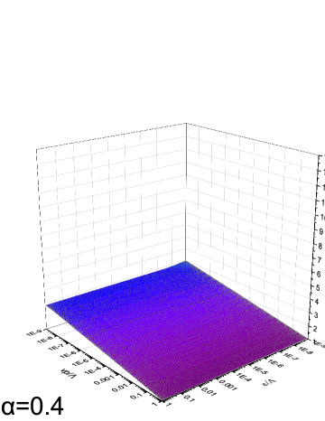
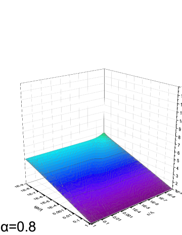
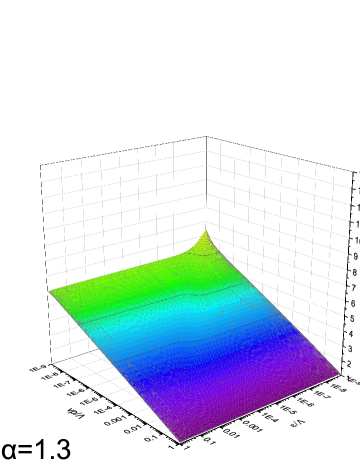
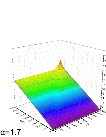
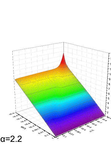
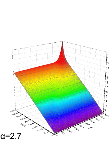
Figure 1: The energy-momentum dependence of renormalized velocity $v_{\mathrm{R}}(\varepsilon,\mathbf{p})$ obtained by using the full fermion-boson vertex function for $\alpha=0.4$, $\alpha=0.8$, $\alpha=1.3$, $\alpha=1.7$, $\alpha=2.2$, and $\alpha=2.7$. Over a wide range of $\varepsilon$ and $\mathbf{p}$, $v_{\mathrm{R}}(\varepsilon,\mathbf{p})$ exhibits a logarithmic dependence on $|\mathbf{p}|$ but is nearly independent of $\varepsilon$. Close to the IR cutoffs of $\varepsilon$ and $\mathbf{p}$, $v_{\mathrm{R}}(\varepsilon,\mathbf{p})$ appears to deviate from the normal behavior and rises abruptly. The origin of such an abrupt rise is explained in the main text.

We first analyze the behavior of fermion velocity renormalization. For concreteness, here we take the UV cutoff Elias11 as $\Lambda=2.0$ eV. It is important to emphasize that the solutions are independent of the value of $\Lambda$. Here, we choose six different values of $\alpha$: $\alpha=0.4$ (graphene on BN substrate), $\alpha=0.8$ (graphene on SiO₂ substrate), $\alpha=1.3$, $\alpha=1.7$, $\alpha=2.2$ (suspended graphene), and $\alpha=2.7$. After solving the most generic equations given by Eqs. (166-168) without making any approximation, we extract the full energy-momentum dependence of the renormalized velocity

$$\frac{v_{\mathrm{R}}(p)}{v}=\frac{A_{1}(p)}{A_{0}(p)}.$$ (172)

from the numerical solutions of $A_{0}(p)$ and $A_{1}(p)$ and show the results in Fig. 1. $m(p)$ has only a zero solution. To the best of our knowledge, the accurate energy-momentum dependence of $v_{\mathrm{R}}(p)$ has never been obtained previously. Here it is convenient to introduce the symbol $\varepsilon$ to denote $-ip_{0}$. At a fixed $\varepsilon$, $v_{\mathrm{R}}(\mathbf{p})$ exhibits a logarithmic dependence on $|\mathbf{p}|$ within a wide range of $|\mathbf{p}|$. These results are qualitatively well consistent with experimental observations of renormalized velocity Elias11 ; Lanzara11 ; Chae12 . It seems incredible that the function $v_{\mathrm{R}}(\mathbf{p})$ obtained by solving the exact DS equation of $G(p)$ displays the same logarithmic behavior obtained in first-order ($O(\alpha)$) perturbative calculations. This perfectly explains why existing experimental data fit well with the $O(\alpha)$ result in graphene materials that actually have a relatively large $\alpha$ (comparing to $\alpha=1/137$ in QED₄).

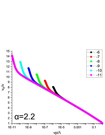
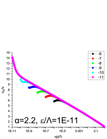
Figure 2: Renormalized velocity obtained by using different IR cutoffs at $\alpha=2.2$. Left panel: The IR cutoff of $\varepsilon$ is equal to that of $v|\mathbf{p}|$. Here, $\varepsilon$ is assumed to take the value of its IR cutoff. Six different IR cutoffs (relative to UV cutoff) are considered: $10^{-6}$, $10^{-7}$, $10^{-8}$, $10^{-9}$, $10^{-10}$, and $10^{-11}$. The logarithmic $|\mathbf{p}|$-dependence of $v_{\mathrm{R}}(\mathbf{p})$ extends for several orders of magnitude of scaled momentum. Close to IR cutoffs, $v_{\mathrm{R}}(\mathbf{p})$ seems to deviate from the standard logarithmic behavior. However, such a seeming deviation is an artifact and the logarithmic behavior is always extended to lower energy and momentum region as IR cutoff is decreasing. Right panel: the energy $\varepsilon$ is fixed at $\varepsilon/\Lambda=10^{-11}$, which also sets its IR cutoff, and the IR cutoff of $v|\mathbf{p}|$ takes six different values. The logarithmic behavior continues going leftwards with lowering IR cutoff of $v|\mathbf{p}|$.

According to Fig. 1, it turns out that $v_{\mathrm{R}}(\varepsilon,\mathbf{p})$ deviates from logarithmic $|\mathbf{p}|$-dependence and $\varepsilon$-independence in the region of small $\varepsilon$ and small $|\mathbf{p}|$ and appears to be considerably increased as $\varepsilon$ and $|\mathbf{p}|$ decrease. We emphasize that such an abrupt deviation is unphysical and stems from the infrared (IR) cutoffs that inevitably exist in practical numerical calculations. This can be understood as follows. In solid state physics, the metallic state is usually described by the jellium model, which assumes that the positive charges are uniformly distributed in space so as to maintain the global neutrality of the system. Aside from the free part (kinetic term) $H_{0}$, the total Hamiltonian contains three interaction terms: $H_{C}$ for Coulomb interaction between electrons, $H_{B}$ for the electrostatic energy of the uniform positive background, and $H_{EB}$ for the interaction energy between the electrons and the background. The term $H_{C}$, which sums over all the possible values of transferred momentum $\mathbf{q}$, is further divided into two parts: $H_{C}(\mathbf{q})=H_{C}(\mathbf{q}=0)+\sum_{\mathbf{q}\neq 0}H_{C}(\mathbf{q})$. It is easy to check Mahan that $H_{C}(\mathbf{q}=0)+H_{B}+H_{EB}=0$. As a result, one can omit all the contributions from positive background and at the same time remove the $\mathbf{q}=0$ contribution from the effective Lagrangian density. That means, $\mathbf{q}$ appearing in the boson propagator $D_{0}(q)\equiv D_{0}(q_{0},\mathbf{q})$ can be made arbitrarily small but cannot be set to zero. In the process of doing numerical calculations, it is always necessary to choose an IR cutoff $\Lambda_{\mathrm{IR}}^{\mathbf{q}}$ for $\mathbf{q}$. The contributions from the range of $|\mathbf{q}|\in(0,\Lambda_{\mathrm{IR}}^{\mathbf{q}})$ are always neglected. Since $D_{0}(\mathbf{q})$ is inversely proportional to $|\mathbf{q}|$, smaller $|\mathbf{q}|$ gives rise to a larger contribution to the fermion self-energy. This is a salient feature of long-range interaction. On the one hand, it indicates that large-$|\mathbf{q}|$ processes are unimportant and ensures that the results are independent of the specific value of UV cutoff. On the other hand, it implies that the neglected contributions from the range $(0,\Lambda_{\mathrm{IR}}^{\mathbf{q}})$ are indeed not small, which explains why an abrupt deviation from the standard logarithmic behavior emerges as $\varepsilon$ and $|\mathbf{p}|$ are close to their IR cutoffs. We choose six different values of $\Lambda_{\mathrm{IR}}$ for $|\mathbf{p}|$. We see from Fig. 2 that decreasing the IR cutoffs of $\varepsilon$ and $|\mathbf{p}|$ always extends the logarithmic behavior into the region of lower momenta. If we fix the fermion energy at $\epsilon/\Lambda=10^{-11}$ and choose UV cutoff $\Lambda=2.0$ eV, the logarithmic velocity renormalization holds over a wide momentum range $v|\mathbf{p}|\in[2.0\times 10^{-10}\mathrm{eV},2.0\mathrm{eV}]$, as shown in the right panel of Fig. 2. Of course we can further decrease the value of $\Lambda_{\mathrm{IR}}$, which would extend the logarithmic behavior into lower momenta.

The logarithmic velocity renormalization would be eventually altered as $|\mathbf{p}|$ becomes very small. This is because the renormalized velocity $v_{\mathrm{R}}$ cannot be greater than the speed of light $c$. When $v_{\mathrm{R}}$ is increased to a magnitude close to $c$, the electromagnetic radiation effect becomes significant and the non-relativistic model of Coulomb interaction between Dirac fermions should be replaced with the fully relativistic $(1+2)$-dimensional QED. As $v_{\mathrm{R}}\rightarrow c$, the corrections to fermion velocity due to the longitudinal (Coulomb-type) and transverse components of gauge field cancel each other, leaving the fermion velocity unrenormalized Vafek07 . But $v_{\mathrm{R}}\rightarrow c$ only at extremely low energies, which can never be realized in graphene materials. Thus the logarithmic velocity renormalization is robust at energy scales accessible to experiments.

Although the inclusion of exact vertex function leads to the same logarithmic $\mathbf{p}$-dependence of $v_{\mathrm{R}}(\mathbf{p})$ as $O(\alpha)$ order calculations, it would be false to say that vertex corrections are not important. To demonstrate the impact of vertex corrections, we also have solved the equations of $A_{0}(p)$ and $A_{1}(p)$ by using the bare vertex, with results being presented in Fig. 3. Comparing Fig. 3 to Fig. 1, we find that $v_{\mathrm{R}}(\mathbf{p})$ exhibits a logarithmic $\mathbf{p}$-dependence at a fixed $\varepsilon$ no matter whether bare vertex or full vertex is utilized. However, the magnitude of $v_{\mathrm{R}}(\varepsilon,\mathbf{p})$ at any given point $(\varepsilon,|\mathbf{p}|)$ is significantly increased due to the inclusion of vertex corrections. In addition, we observe from Fig. 3 that $v_{\mathrm{R}}(\varepsilon,\mathbf{p})$ is nearly energy independent if the exact vertex function is adopted. In contrast, ignoring the vertex corrections would lead to an incorrect result that $v_{\mathrm{R}}(\varepsilon,\mathbf{p})$ is strongly energy dependent. All these results point to conclusions that the vertex corrections do play a vital role and should be seriously taken into account.

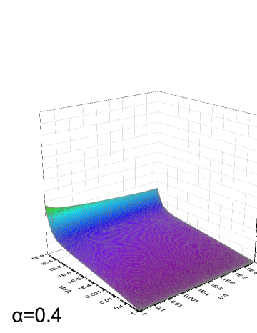
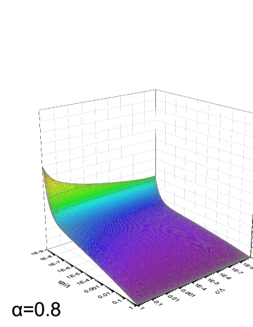
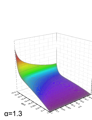
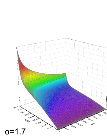
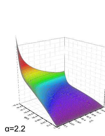
Figure 3: The energy-momentum dependence of $v_{\mathrm{R}}(\varepsilon,\mathbf{p})$ obtained by using the bare vertex function and the RPA-form of boson propagator $D_{\mathrm{RPA}}(k-p)$ for $\alpha=0.4$, $\alpha=0.8$, $\alpha=1.3$, $\alpha=1.7$, $\alpha=2.2$, and $\alpha=2.7$. $v_{\mathrm{R}}(\varepsilon,\mathbf{p})$ shows a strong dependence on $\varepsilon$, which, however, is an artifact of incorrect approximation.

Next we discuss the possibility of excitonic gap generation. To elaborate how $\alpha_{c}$ is influenced by various ingredients, we have solved the equations of $A_{0}(p)$, $A_{1}(p)$, and $m(p)$ under several different approximations. For instance, we found $\alpha_{c}\approx 1.0$ if the bare vertex $\gamma^{0}$ and the free boson propagator $D_{0}(q)$ are employed. If we use bare vertex $\gamma^{0}$ but promote $D_{0}(q)$ to RPA propagator $D_{\mathrm{RPA}}(q)$, then $\alpha_{c}\approx 3.9$. If we use $D_{\mathrm{RPA}}(q)$ and the leading term of the so-called Ball-Chiu Ansatz of vertex function (see WangLiu12 ; Carrington16 for an explanation), we found $\alpha_{c}\approx 2.9$. Apparently, the value of $\alpha_{c}$ is very sensitive to the chosen approximation. In order to eliminate the unpleasant ambiguity in results of $\alpha_{c}$, it is important to go beyond all approximations and adopt the exact vertex function derived from coupled WTIs. We have solved the most generic equations (166)-(168) and found that no excitonic gap is generated for $\alpha<5$. An immediate indication is that the semimetallic ground state of graphene is surprisingly robust against Coulomb interaction.

Resistivity measurements Elias11 ; Mayorov12 have been performed to detect the possible existence of excitonic insulating transition in clean graphene. No sign of insulating state was found Elias11 ; Mayorov12 down to roughly $1$ K. Indeed, thus far there is no experimental signature of the excitonic-type pairing instability in graphene. Our theoretical results are consistent with the experimental situation.

When $\alpha>5$, anomalous behaviors emerge. While the two functions $A_{0}(p)$ and $A_{1}(p)$ exhibit regular behaviors (without singularities) and lead to logarithmic velocity renormalization for $\alpha<5$, they no longer have stable solutions once $\alpha$ exceeds $5$. It turns out that the system undergoes an instability as $\alpha$ is increased across $5$. But the nature of such an instability remains elusive. The transition into an excitonic insulator can be directly precluded since the equation of excitonic gap always has a vanishing solution (i.e., $m=0$) for all values of $\alpha$. Further investigations are called for to uncover the nature of such an instability.

If two-component spinor and $2\times 2$ gamma matrices are utilized to describe Dirac fermions, the integral equations of $A_{0}(p)$ and $A_{1}(p)$ would still be given by Eqs. (166) and (167). All the results about the velocity renormalization would not be changed. The only difference is that chiral symmetry cannot be explicitly defined.

As shown in Ref. Liu19 , one can make proper use of the solutions of $A_{0}(p)$ and $A_{1}(p)$ to explore the properties of the boson. Substituting the full fermion propagator $G(p)$ and the full vertex function $\Gamma_{\mathrm{int}}(k,p)=D_{0}(q)\Upsilon_{\gamma^{0}}(k,p)D^{-1}(q)$ into the DS equation of boson propagator $D(q)$, we find

$$D^{-1}(q)=D^{-1}_{0}(q)-iND_{0}(q)D^{-1}(q)\int\frac{d^{3}k}{(2\pi)^{3}}{\mathrm{Tr}}\left[\gamma^{0}G(k+q)\Upsilon_{\gamma^{0}}(k,p)G(k)\right],$$ (173)

which can be further written as

$$D(q)=D_{0}(q)+iND_{0}^{2}(q)\int\frac{d^{3}k}{(2\pi)^{3}}{\mathrm{Tr}}\left[\gamma^{0}G(k+q)\Upsilon_{\gamma^{0}}(k,p)G(k)\right].$$ (174)

Then the full polarization function $\Pi(q)$ can be calculated from $D(q)$, based on the relation

$$\Pi(q)=D_{0}^{-1}(q)-D^{-1}(q).$$ (175)

This $\Pi(q)$ is exact and can be used to investigate such effects as plasmon and Friedel oscillation, which is out of the scope of this paper.

In this paper we consider only undoped graphene. However, the graphene samples prepared in laboratory are always doped. Thus the Fermi level is not exactly located at the neutral Dirac point. It was found Elias11 ; Lanzara11 ; Chae12 that the renormalized velocity displays a logarithmic dependence on carrier density. As elaborated by Barnes et al. Barnes14 , although the density actually becomes unimportant as the temperature scale $k_{B}T$ is greater than the Fermi energy $E_{F}$, the results obtained at Dirac point cannot be directly used to account for the density dependence of renormalized velocity. To explain the observed density dependence at a quantitative level, it is necessary to extend the analysis of undoped graphene to the case of doped graphene DasSarma13 . The impact of finite carrier density can be taken into account by adding a finite chemical potential $\mu$ to the free fermion Hamiltonian via the replacement

$$H_{f}=\sum_{\sigma=1}^{N}\bar{\psi}_{\sigma}\gamma\cdot\partial\psi_{\sigma}\rightarrow H_{f}-\mu\sum_{\sigma=1}^{N}\bar{\psi}_{\sigma}\gamma^{0}\psi_{\sigma}.$$ (176)

Then the free fermion propagator becomes

$$G_{0}(p,\mu)\equiv G_{0}(p_{0},\mathbf{p},\mu)=\frac{1}{\gamma^{0}\left(p_{0}-\mu\right)-v\mathbf{\gamma}\cdot\mathbf{p}}.$$ (177)

The generalized WTIs and the equations of $A_{0}(p,\mu)$, $A_{1}(p,\mu)$, and $m(p,\mu)$ can be similarly derived and solved, following the calculational procedure developed in the case of $\mu=0$, which will allow for a more quantitative comparison between field-theoretic results and experiments. This issue is out of the scope of this paper and will be addressed systematically in a forthcoming work.

If graphene is made anisotropic, the free and full fermion propagators would take the forms

$$G_{0}(p) = \frac{1}{\gamma^{0}p_{0}-v_{1}\gamma^{1}p_{1}-v_{2}\gamma^{2}p_{2}},$$ (178)

$$G(p) = \frac{1}{A_{0}(p)\gamma^{0}p_{0}-A_{1}(p)\gamma^{1}p_{1}-A_{2}(p)\gamma^{2}p_{2}+m(p)}.$$ (179)

The interaction effects are now embodied in the three functions $A_{0,1,2}(p)$ and $m(p)$. The renormalization of velocities $v_{1}$ and $v_{2}$ can be analyzed based on $A_{1}(p)/A_{0}(p)$ and $A_{2}(p)/A_{0}(p)$, respectively.

The same calculational procedure can be applied to study the fermion-phonon coupling in graphene by replacing the bare Coulomb interaction function $D_{0}(q)=\frac{2\pi e^{2}}{v\epsilon|\mathbf{q}|}$ with the free phonon propagator $D_{0}(q)=-\frac{\Omega_{\mathbf{q}}}{q_{0}^{2}-\Omega_{\mathbf{q}}^{2}}$. Application of the approach to $(1+3)$-dimensional Dirac semimetal is straightforward. In this case, the current vertex function should be computed based on the expressions shown in Sec. VI.2.

IX Summary and Discussion

In this paper we have developed a powerful non-perturbative DS equation approach to study the strong coupling of massless Dirac fermions to a scalar boson. The full vertex function of fermion-boson coupling is incorporated into the DS equation of full fermion propagator by solving a number of coupled WTIs that are derived rigorously from several symmetric and asymmetric global U(1) transformations. Based on this result, we prove that the DS equation of full fermion propagator is entirely self-closed and can be numerically solved. After solving this DS equation, the fermion damping, the fermion velocity renormalization, and the possible excitonic pairing can be investigated in a self-consistent way. In using our approach, there is no need to expand physical quantities into powers of small parameter. All the interaction-induced effects on Dirac fermions are extracted from the solutions of exact DS equation(s). Therefore, the results are reliable no matter whether the fermion-boson coupling is weak or strong.

We have applied our approach to revisit the strong Coulomb interaction in undoped graphene and solved the exact self-consistent integral equations of wave function renormalizations $A_{0,1}(p)$ and excitonic gap $m(p)$. Our numerical results indicate that the renormalized fermion velocity displays a logarithmic momentum dependence over a wide range of momentum at a fixed energy, and that the Coulomb interaction cannot open an excitonic gap. These results are qualitatively in agreement with experiments. More in-depth theoretical analysis is required to carry out a more quantitative explanation of relevant experiments. Potential directions of future research include analyzing the carrier-density dependence of renormalized fermion velocity and computing a number of observable quantities, such as specific heat and optical conductivity.

Our approach is applicable to long-range Coulomb interaction and fermion-phonon interaction in both $(1+2)$ and $(1+3)$ dimensions. But, the approach is no longer exact if the boson action has a self-coupling term, such as $\phi^{4}$. We emphasize that the coupled WTIs derived in Sec. IV and the current vertex functions obtained in Secs. V and VI are always valid, irrespective of whether there is a self-interaction of scalar boson. This is because the WTIs originate from the variation of the action under infinitesimal transformations of the fermion field. The real difficulty brought by the boson self-interaction is that the identity given by Eq. (146) would have a complicated additional term. In order to adopt our approach to investigate the fertile quantum critical phenomena of Dirac fermion systems Kim08 ; Wangmit17 ; Pan18 ; Liunematic12 ; Wang19 ; Xiao19 ; Lang19 ; LeeSS07 ; Grover14 ; Jian15 ; Liu19npj , we need to find a controllable method to either exactly or approximately treat such an additional term. This problem will be studied in a subsequent project.

We believe that the DS equation approach can also be applied to study the superconducting instability of Dirac fermion systems, mediated by phonons or other bosonic modes, and the interplay between superconductivity and CDW. The Nambu spinor of Dirac fermions usually has eight components, thus the structure of WTIs would be very complicated. One might have to solve eight or even sixteen coupled WTIs to obtain one specific current vertex function.

Appendix A Definitions of some matrices

Here we present the conventions and define all the matrices used in the paper.

The metric tensor in $(1+2)$ and $(1+3)$ dimensions are

$$g_{\mu\nu}=\left({\begin{array}[]{*{20}{c}}1&0&0\\ 0&-1&0\\ 0&0&-1\end{array}}\right),\quad g_{\mu\nu}=\left({\begin{array}[]{*{20}{c}}1&0&0&0\\ 0&-1&0&0\\ 0&0&-1&0\\ 0&0&0&-1\end{array}}\right).$$ (187)

Three- and four-vectors for coordinate and momentum are written as $x^{\mu}=(x^{0},x^{i})=(x^{0},\mathbf{x})$ and $p^{\mu}=(p^{0},p^{i})=(p^{0},\mathbf{p})$. The following relations are frequently used:

$$x_{\mu}=g_{\mu\nu}x^{\nu},\quad p_{\mu}=g_{\mu\nu}p^{\nu},\quad\gamma_{\mu}=g_{\mu\nu}\gamma^{\nu}.$$ (188)

Standard Pauli matrices are

$$\tau^{1}={\begin{pmatrix}0&1\\ 1&0\end{pmatrix}},\quad\tau^{2}={\begin{pmatrix}0&-i\\ i&0\end{pmatrix}},\quad\tau^{3}={\begin{pmatrix}1&0\\ 0&-1\end{pmatrix}}.$$

In both $(1+2)$ and $(1+3)$ dimensions, we will use the following five $4\times 4$ gamma matrices:

$$\gamma^{0}=\gamma_{0}={\begin{pmatrix}\tau^{3}&0\\ 0&-\tau^{3}\end{pmatrix}},\quad\gamma^{1}=-\gamma_{1}={\begin{pmatrix}i\tau^{2}&0\\ 0&-i\tau^{2}\end{pmatrix}},\quad\gamma^{2}=-\gamma_{2}={\begin{pmatrix}-i\tau^{1}&0\\ 0&i\tau^{1}\end{pmatrix}},$$ (189)

and

$$\gamma^{3}=-\gamma_{3}=-i{\begin{pmatrix}0&1\\ 1&0\end{pmatrix}},\quad\gamma^{5}\equiv i\gamma^{0123}=i\gamma^{0}\gamma^{1}\gamma^{2}\gamma^{3}=i{\begin{pmatrix}0&1\\ -1&0\end{pmatrix}}.$$ (190)

To derive the coupled WTIs in Sec. V and Sec. VI, we need to construct several $4\times 4$ matrices:

$$\sigma^{01}=\frac{i}{2}[\gamma^{0},\gamma^{1}]=i\gamma^{0}\gamma^{1}={\begin{pmatrix}i\tau^{1}&0\\ 0&i\tau^{1}\end{pmatrix}},$$ (191)

$$\sigma^{02}=\frac{i}{2}[\gamma^{0},\gamma^{2}]=i\gamma^{0}\gamma^{2}={\begin{pmatrix}i\tau^{2}&0\\ 0&i\tau^{2}\end{pmatrix}},$$ (192)

$$\sigma^{12}=\frac{i}{2}[\gamma^{1},\gamma^{2}]=i\gamma^{1}\gamma^{2}={\begin{pmatrix}\tau^{3}&0\\ 0&\tau^{3}\end{pmatrix}},$$ (193)

$$\{{\sigma^{01},\gamma^{2}}\}=2\tau^{3}\otimes I=2{\begin{pmatrix}I&0\\ 0&-I\end{pmatrix}},$$ (194)

$$\{{\sigma^{02},\gamma^{1}}\}=-2\tau^{3}\otimes I=2{\begin{pmatrix}-I&0\\ 0&I\\ \end{pmatrix}},$$ (195)

$$\{{\sigma^{12},\gamma^{0}}\}=2\tau^{3}\otimes I=2{\begin{pmatrix}I&0\\ 0&{-I}\end{pmatrix}}.$$ (196)

In $(1+3)$ dimensions, we also need three additional matrices:

$$\sigma^{03} = \frac{i}{2}[\gamma^{0},\gamma^{3}]=i\gamma^{0}\gamma^{3}=\begin{pmatrix}0&\tau^{3}\\ -\tau^{3}&0\end{pmatrix},$$ (197)

$$\sigma^{13} = \frac{i}{2}[\gamma^{1},\gamma^{3}]=i\gamma^{1}\gamma^{3}=\begin{pmatrix}0&i\tau^{2}\\ -i\tau^{2}&0\end{pmatrix},$$ (198)

$$\sigma^{23} = \frac{i}{2}[\gamma^{2},\gamma^{3}]=i\gamma^{2}\gamma^{3}=\begin{pmatrix}0&-i\tau^{1}\\ i\tau^{1}&0\end{pmatrix}.$$ (199)

As mentioned in Sec. II, one can alternatively use $2\times 2$ matrices to describe two-component spinor in $(1+2)$ dimensions. This representation would lead to the same results as four-component spinor representation, if we are not intended to consider chiral symmetry (breaking). Although we adopt four-component spinor throughout the main text of the paper, here for completeness we also show how our approach works if two-component spinor is adopted. One can choose

$$\gamma^{0}=\tau^{3},\quad\gamma^{1}=i\tau^{1},\quad\gamma^{2}=i\tau^{2}.$$ (200)

These three matrices also satisfy $\{\gamma^{\mu},\gamma^{\nu}\}=2g^{\mu\nu}$. The following three matrices are needed:

$$\sigma^{01}=-i\gamma^{0}\gamma^{1}=-i\tau^{2},\quad\sigma^{02}=-i\gamma^{0}\gamma^{2}=-i\tau^{1},\quad\sigma^{12}=i\gamma^{1}\gamma^{2}=\tau^{3}.$$ (201)

The corresponding WTIs can be readily obtained by substituting the above expressions of $\gamma^{0}$, $\gamma^{1}$, $\gamma^{2}$, $\sigma^{01}$, $\sigma^{02}$, and $\sigma^{12}$ into the general expressions of Eqs. (57) and (58).

Appendix B Derivation of Dyson-Schwinger equations

In this Appendix we derive the DS equations of fermion and boson propagators within the functional-integral formalism of quantum field theory. Similar derivations have previously be presented in Ref. Liu19 . However, we feel it helpful to provide some crucial calculational details here.

The starting point is the partition function

$$\mathcal{Z}[J,{\bar{\eta}},\eta] = \int\mathcal{D}\phi\mathcal{D}\psi\mathcal{D}{\bar{\psi}}e^{i\int dx[{\mathcal{L}}+J\phi+{\bar{\eta}}\psi+{\bar{\psi}}\eta)}$$ (202)

$$= e^{iW[J,{\bar{\eta}},\eta]}.$$

The Lagrange density is given by

$$\mathcal{L}=\sum^{N}_{\sigma=1}\left[{\bar{\psi}}_{\sigma}(x)i\gamma^{\mu}\partial_{\mu}\psi_{\sigma}(x)+g\phi(x){\bar{\psi}}_{\sigma}(x)\gamma^{m}\psi_{\sigma}(x)\right]+\frac{1}{2}\phi(x)\mathbb{D}\phi(x).$$ (203)

The average of an arbitrary operator $\mathcal{O}$ is defined as

$$\langle\mathcal{O}(x)\rangle_{J}=\frac{[[O(x)]]_{J}}{[[1]]_{J}},$$ (204)

where $[[1]]_{J}$ is just the partition function $\mathcal{Z}$ and

$$[[O(x)]]_{J}=\int\mathcal{D}\phi\mathcal{D}\psi\mathcal{D}{\bar{\psi}}e^{i\int dx[\mathcal{L}+J\phi+{\bar{\eta}}\psi+{\bar{\psi}}\eta]}O(x).$$ (205)

Here we use one single subscript $J$ to stand for all the possible external sources, i.e., $\langle\mathcal{O}\rangle_{J}\equiv\langle\mathcal{O}\rangle_{J,{\bar{\eta}},\eta}$.

B.1 Dyson-Schwinger equation of boson propagator

Since $\delta\mathcal{Z}=0$ under an arbitrary infinitesimal variation $\delta\phi$, we have

$$0 = \int\mathcal{D}\phi\mathcal{D}\psi\mathcal{D}{\bar{\psi}}\left[\frac{\delta\mathcal{L}}{\delta\phi(x)}+J(x)\right]e^{i\int dx[\mathcal{L}+J\phi+{\bar{\eta}}\psi+{\bar{\psi}}\eta]}$$ (206)

$$= \left[\frac{\delta\mathcal{L}}{\delta\phi(x)}\left(\frac{\delta}{i\delta J},\frac{\partial}{i{\bar{\eta}}_{\sigma}},-\frac{\delta}{i\delta\eta_{\sigma}}\right)+J\right]\mathcal{Z}[J,{\bar{\eta}},\eta].$$

Since

$$\frac{\delta\mathcal{L}}{\delta\phi(x)}=g\sum^{N}_{\sigma=1}{\bar{\psi}}_{\sigma}(x)\gamma^{m}\psi_{\sigma}(x)+\mathbb{D}\phi(x),$$ (207)

one can verify that

$$J(x)\mathcal{Z}+\mathbb{D}\frac{\delta\mathcal{Z}}{i\delta J(x)}+g\sum^{N}_{\sigma=1}\frac{\delta}{-i\delta\eta_{\sigma}(x)}\gamma^{m}\frac{\delta}{i\delta{\bar{\eta}}_{\sigma}(x)}\mathcal{Z}=0.$$ (208)

Dividing this equation by $\mathcal{Z}$ yields

$$J(x)+\mathbb{D}\frac{\delta W}{\delta J(x)}+\frac{g}{\mathcal{Z}}\sum^{N}_{\sigma=1}\frac{\delta}{\delta\eta_{\sigma}(x)}\gamma^{m}\frac{\delta}{\delta{\bar{\eta}}_{\sigma}(x)}e^{iW}=0.$$ (209)

The last term of the l.h.s. of the above equation is

$$\frac{g}{\mathcal{Z}}\frac{\delta}{\delta\eta_{\sigma}(x)}\gamma^{m}\frac{\delta}{\delta{\bar{\eta}}_{\sigma}(x)}e^{iW}=-ig{\mathrm{Tr}}[\gamma^{m}\frac{\delta^{2}W}{\delta{\bar{\eta}}_{\sigma}(x)\delta\eta_{\sigma}(y)}]-g\frac{\delta W}{\delta\eta_{\sigma}(x)}\gamma^{m}\frac{\delta W}{\delta{\bar{\eta}}_{\sigma}(x)}.$$ (210)

The second term of the r.h.s vanishes as the fields are set to be zero.

To proceed, we define the following Legendre transformation

$$\Xi(\phi,\psi,{\bar{\psi}})=W(J,{\bar{\eta}},\eta)-\sum^{N}_{\sigma=1}\int dx\left[J\phi+{\bar{\psi}}_{\sigma}\eta_{\sigma}+{\bar{\eta}}_{\sigma}\psi_{\sigma}\right].$$ (211)

It is known Itzykson that the following identities hold

$$\phi(x)=\frac{\delta W}{\delta J(x)},\quad\psi_{\sigma}(x)=\frac{\delta W}{\delta{\bar{\eta}}_{\sigma}(x)},\quad{\bar{\psi}}_{\sigma}(x)=-\frac{\delta W}{\delta\eta_{\sigma}(x)}$$

$$J(x)=-\frac{\delta\Xi}{\delta\phi(x)},\quad\eta_{\sigma}(x)=-\frac{\delta\Xi}{\delta{\bar{\psi}}_{\sigma}(x)},\quad{\bar{\eta}}_{\sigma}(x)=\frac{\delta\Xi}{\delta\psi(x)}.$$ (212)

The boson propagator and its inverse are defined as

$$D(x,y) = -\frac{\delta^{2}W}{\delta J(x)\delta J(y)}=-\frac{\delta\phi(y)}{\delta J(x)}=-i\langle\phi(x)\phi(y)\rangle_{c},$$ (213)

$$D^{-1}(x,y) = \frac{\delta^{2}\Xi}{\delta\phi(x)\delta\phi(y)}=-\frac{\delta J(x)}{\delta\phi(y)}.$$ (214)

It is easy to check that

$$\int dyD(x,y)D^{-1}(y,z)=\int dy\frac{-\delta^{2}W}{\delta J(x)\delta J(y)}\frac{\delta^{2}\Xi}{\delta\phi(y)\delta\phi(z)}=\int dy\frac{\delta\phi(x)}{\delta J(y)}\frac{\delta J(y)}{\delta\phi(z)}=\delta(x-z).$$ (215)

Similarly, for each flavor $\sigma$ of the fermion propagator and its inverse we have

$$G_{\alpha\beta}(x,y)=\frac{\delta^{2}W}{\delta{\bar{\eta}}_{\alpha}(x)\delta\eta_{\beta}(y)}=-\frac{\delta\psi_{\alpha}(x)}{\delta\eta_{\beta}(y)}=-\frac{\delta{\bar{\psi}}_{\beta}(y)}{\delta{\bar{\eta}}_{\alpha}(x)}=-i\langle\psi_{\alpha}(x){\bar{\psi}}_{\beta}(y)\rangle_{c},$$ (216)

$$G_{\beta\rho}^{-1}(y,z)=-\frac{\delta^{2}\Xi}{\delta{\bar{\psi}}_{\beta}(y)\delta\psi_{\rho}(z)}=-\frac{\delta\eta_{\beta}(y)}{\delta\psi_{\rho}(z)}=-\frac{\delta{\bar{\eta}}_{\rho}(z)}{\delta{\bar{\psi}}_{\beta}(y)}.$$ (217)

Then they fulfill the relation

$$\int G_{\alpha\beta}(x,y)G_{\beta\rho}^{-1}(y,z)dy=\delta(x-z)\delta_{\alpha\rho}.$$ (218)

Eq. (B8) can be re-written as

$$J(x)=-\mathbb{D}\frac{\delta W}{\delta J(x)}+ig\sum^{N}_{\sigma=1}{\mathrm{Tr}}\left[\gamma^{m}\frac{\delta^{2}W}{\delta{\bar{\eta}}_{\sigma}(x)\delta\eta_{\sigma}(x)}\right],$$ (219)

Making the variation $\frac{\delta}{\delta J(y)}$ on both sides of Eq. (B18) we obtain

$$\delta(x-y)=\mathbb{D}D(x-y)+ig\sum^{N}_{\sigma=1}\mathrm{Tr}\left[\gamma^{m}\frac{\delta^{3}W}{\delta J(y)\delta{\bar{\eta}}_{\sigma}(x)\delta\eta_{\sigma}(x)}\right].$$ (220)

Using the relation of Eq. (139), now we can write the DS equation of boson propagator in the form

$$\delta(x-y)=\mathbb{D}D(x-y)-ig^{2}N\int dx^{\prime}dy^{\prime}dz^{\prime}{\mathrm{Tr}}\left[\gamma^{m}D(y,x^{\prime})G(x,y^{\prime})\Gamma_{\mathrm{int}}(y^{\prime}-x^{\prime},x^{\prime}-z^{\prime})G(z^{\prime},x)\right],$$

which in the momentum space becomes

$$D^{-1}(q)=D_{0}^{-1}(q)-ig^{2}N\int\frac{dk}{(2\pi)^{(1+d)}}\mathrm{Tr}\left[\gamma^{m}G(k+q)\Gamma_{\mathrm{int}}(k+q,k)G(k)\right].$$ (222)

B.2 Dyson-Schwinger equation of fermion propagator

The DS equation of fermion propagator can be similarly derived.

Since $\delta\mathcal{Z}=0$ under an arbitrary infinitesimal variation $\delta\psi$, we obtain an equation

$$0=\int\mathcal{D}\phi\mathcal{D}\psi\mathcal{D}{\bar{\psi}}\left[\frac{\delta\mathcal{L}}{\delta{\bar{\psi}}(x)}\left(\frac{\delta}{i\delta J},\frac{\delta}{i\delta{\bar{\eta}}_{\sigma}},\frac{\delta}{-i\delta\eta_{\sigma}}\right)+\eta_{\sigma}(x)\right]\mathcal{Z}(J,{\bar{\eta}},\eta),$$ (223)

which implies that

$$\eta_{\sigma}(x)\mathcal{Z}+i\gamma^{\mu}{\partial_{\mu}}\mathcal{Z}\frac{\delta W}{\delta{\bar{\eta}}_{\sigma}(x)}+g\frac{\delta}{i\delta J(x)}\gamma^{m}\left(\mathcal{Z}\frac{\delta W}{\delta{\bar{\eta}}_{\sigma}(x)}\right)=0.$$ (224)

Operating the functional derivative $\frac{\delta}{\delta\eta_{\sigma}(y)}$ on both sides of the above equation and then setting $\psi={\bar{\psi}}=0$, one finds

$$\delta(x-y)\mathcal{Z}+i\gamma^{\mu}{\partial_{\mu}}\mathcal{Z}\frac{\delta^{2}W}{\delta\eta_{\sigma}(y)\delta{\bar{\eta}}_{\sigma}(x)}+g\frac{\delta}{i\delta J(x)}\gamma^{m}\mathcal{Z}\frac{\delta^{2}W}{\delta\eta_{\sigma}(y)\delta{\bar{\eta}_{\sigma}}(x)}=0,$$ (225)

which in turn leads to for each flavor $\sigma$

$$i\gamma^{\mu}{\partial_{\mu}}G(x,y)-ig\gamma^{m}\frac{\delta^{3}W}{\delta J(x)\delta{\bar{\eta}}_{\sigma}(x)\delta\eta_{\sigma}(y)}=\delta(x-y).$$ (226)

The second term of the l.h.s of above equation can be calculated with the help of Eq. (139). Fourier transformation of the above equation yields the following equation

$$\gamma^{\mu}p_{\mu}G(p)+ig^{2}\int\frac{dk}{(2\pi)^{(1+d)}}\gamma^{m}G(k)D(k-p)\Gamma_{\mathrm{int}}(k,p)G(p)=1,$$ (227)

which can be turned into the DS equation of fermion propagator

$$G^{-1}(p)=G^{-1}_{0}(p)+ig^{2}\int\frac{dk}{(2\pi)^{(1+d)}}\gamma^{m}G(k)D(k-p)\Gamma_{\mathrm{int}}(k,p).$$ (228)

References

- (1) A. A. Abrikosov, L. P. Gor’kov, and I. Y. Dzyaloshinskii, Quantum Field Theoretical Methods in Statistical Physics (Pergamon Press Inc., 1965).
- (2) P. Coleman, Introduction to Many-Body Physics (Cambridge University Press, Cambridge, 2015).
- (3) P. A. Lee, N. Nagaosa, and X.-G. Wen, Rev. Mod. Phys. 78, 17 (2006).
- (4) H. Loehneysen, A. Rosch, M. Vojta, and P. Woelfle, Rev. Mod. Phys. 79, 1015 (2007).
- (5) A. H. Castro Neto, F. Guinea, N. M. R. Peres, K. S. Novoselov, and A. K. Geim, Rev. Mod. Phys. 81, 109 (2009).
- (6) V. N. Kotov, B. Uchoa, V. M. Pereira, F. Guinea, and A. H. Castro Neto, Rev. Mod. Phys. 84, 1067 (2012).
- (7) O. Vafek and A. Vishwanath, Annu. Rev. Condens. Matter Phys. 5, 83 (2014).
- (8) T. O. Wehling, A. M. Black-Schaffer, and A. V. Balatsky, Adv. Phys. 63, 1 (2014).
- (9) N. P. Armitage, E. J. Mele, and A. Vishwanath, Rev. Mod. Phys. 90, 015001 (2018).
- (10) H.-K. Tang, J. N. Leaw, J. N. B. Rodrigues, I. Herbut, P. Sengupta, F. F. Assaad, and S. Adam, Science 361, 570 (2018).
- (11) J. Polchinski, Nucl. Phys. B 422, 617 (1994).
- (12) B. L. Altshuler, L. B. Ioffe, and A. J. Millis, Phys. Rev. B 50, 14048 (1994).
- (13) Y. B. Kim, A. Furusaki, X.-G. Wen, and P.-A. Lee, Phys. Rev. B 50, 17917 (1994).
- (14) D. H. Kim, P.-A. Lee, and X.-G. Wen, Phys. Rev. Lett. 79, 2109 (1997).
- (15) W. Rantner and X.-G. Wen, Phys. Rev. Lett. 86, 3871 (2001).
- (16) J. Rech, C. Pepin, and A. V. Chubukov, Phys. Rev. B 74, 195126 (2006).
- (17) E.-A. Kim, M. J. Lawler, P. Oreto, S. Sachdev, E. Fradkin, and S. A. Kivelson, Phys. Rev. B 77, 184514 (2008).
- (18) M. A. Metlitski and S. Sachdev, Phys. Rev. B 82, 075127 (2010).
- (19) M. A. Metlitski and S. Sachdev, Phys. Rev. B 82, 075128 (2010).
- (20) J. A. Damia, S. Kachru, S. Raghu, and G. Torroba, Phys. Rev. Lett. 123, 096402 (2019).
- (21) S.-S. Lee, Phys. Rev. B 80, 165102 (2009).
- (22) K. S. Novoselov, A. K. Geim, S. V. Morozov, D. Jiang, M. I. Katsnelson, I. V. Grigorieva, S. V. Dubonos, and A. A. Firsov, Nature 438, 197 (2005).
- (23) A. K. Geim and K. S. Novoselov, Nat. Mater. 6, 183 (2007).
- (24) M. Z. Hasan and C. L. Kane, Rev. Mod. Phys. 82, 3045 (2010).
- (25) X.-L. Qi and S.-C. Zhang, Rev. Mod. Phys. 83, 1057 (2011).
- (26) S.-Y. Xu, Y. Xia, L. A. Wray, S. Jia, F. Meier, J. H. Dil, J. Osterwalder, B. Slomski, A. Bansil, H. Lin, R. J. Cava, and M. Z. Hasan, Science 332, 560 (2011).
- (27) T. Sato, K. Segawa, K. Kosaka, S. Souma, K. Nakayama, K. Eto, T. Minami, Y. Ando, and T. Takahashi, Nat. Phys. 7, 840 (2011).
- (28) L. Wu, M. Brahlek, R. V. Aguilar, A. V. Stier, C. M. Morris, Y. Lubashevsky, L. S. Bilbro, N. Bansal, S. Oh, and N. P. Armitage, Nat. Phys. 9, 410 (2013).
- (29) M. Brahlek, N. Bansal, N. Koirala, S.-Y. Xu, M. Neupane, C. Liu, M. Z. Hasan, and S. Oh, Phys. Rev. Lett. 109, 186403 (2012).
- (30) Z. Wang, Y. Sun, X.-Q. Chen, C. Franchini, G. Xu, H. Weng, X. Dai, and Z. Fang, Phys. Rev. B 85, 195320 (2012).
- (31) Z. Wang, H. Weng, Q. Wu, X. Dai, and Z. Fang, Phys. Rev. B 88, 125427 (2013).
- (32) Z. K. Liu, B. Zhou, Y. Zhang, Z. J. Wang, H. M. Weng, D. Prabhakaran, S.-K. Mo, Z. S. Shen, Z. Fang, X. Dai, Z. Hussain, and Y. L. Chen, Science 343, 864 (2014).
- (33) M. Neupane, S.-Y. Xu, R. Sankar, N. Alidoust, G. Bian, C. Liu, I. Belopolski, T.-R. Chang, H.-T. Jeng, H. Lin, A. Bansil, F. Chou, and M. Z. Hasan, Nat. Commun. 5, 3786 (2014).
- (34) Z. K. Liu, J. Jiang, B. Zhou, Z. J. Wang, Y. Zhang, H. M. Weng, D. Prabhakaran, S.-K. Mo, H. Peng, P. Dudin, T. Kim, M. Hoesch, Z. Fang, X. Dai, Z. X. Shen, D. L. Feng, Z. Hussain, and Y. L. Chen, Nat. Mat. 13, 677 (2014).
- (35) S. Borisenko, Q. Gibson, D. Evtushinsky, V. Zabolotnyy, B. Büchner, and R. J. Cava, Phys. Rev. Lett. 113, 027603 (2014).
- (36) L. P. He, X. C. Hong, J. K. Dong, J. Pan, Z. Zhang, J. Zhang, and S. Y. Li, Phys. Rev. Lett. 113, 246402 (2014).
- (37) C. Zhang, Y. Zhang, X. Yuan, S. Lu, J. Zhang, A. Narayan, Y. Liu, H. Zhang, Z. Ni, R. Liu, E. S. Choi, A. Suslov, S. Sanvito, L. Pi, H.-Z. Lu, A. Potter, and F. Xiu, Nature 565, 331 (2019).
- (38) J. González, F. Guinea, and M. A. H. Vozmediano, Phys. Rev. B 59, R2474 (1999).
- (39) E.-G. Moon, C. Xu, Y. B. Kim, and L. Balents, Phys. Rev. Lett. 111, 206401 (2013).
- (40) I. F. Herbut and L. Janssen, Phys. Rev. Lett. 113, 106401 (2014).
- (41) L. Savary, E.-G. Moon, and L. Balents, Phys. Rev. X 4, 041027 (2014).
- (42) L. Janssen and I. F. Herbut, Phys. Rev. B 95, 075101 (2017).
- (43) H. Isobe, B.-J. Yang, A. Chubukov, J. Schmalian, and N. Nagaosa, Phys. Rev. Lett. 116, 076803 (2016).
- (44) J.-R. Wang, G.-Z. Liu, and C.-J. Zhang, Phys. Rev. B 95, 075129 (2017).
- (45) J.-R. Wang, G.-Z. Liu, and C.-J. Zhang, Phys. Rev. B 98, 205113 (2018).
- (46) J.-R. Wang, G.-Z. Liu, and C.-J. Zhang, Phys. Rev. B 99, 195119 (2019).
- (47) S. Han, C. Lee, E.-G. Moon, and H. Min, Phys. Rev. Lett. 122, 187601 (2019).
- (48) J. González, F. Guinea, and M. A. H. Vozmediano, Nucl. Phys. B 424, 595 (1994).
- (49) S. Das Sarma, E. H. Hwang, and W.-K. Tse, Phys. Rev. B 75, 121406(R) (2007).
- (50) M. Polini, R. Asgari, Y. Barlas, T. Pereg-Barnea, and A. H. MacDonald, Solid State Commun. 143, 58 (2007).
- (51) D. T. Son, Phys. Rev. B 75, 235423 (2007).
- (52) O. Vafek, Phys. Rev. Lett. 98, 216401 (2007).
- (53) E. G. Mishchenko, Phys. Rev. Lett. 98, 216801 (2007).
- (54) O. Vafek and M. J. Case, Phys. Rev. B 77, 033410 (2008).
- (55) J. E. Drut and D. T. Son, Phys. Rev. B 77, 075115 (2008).
- (56) M. S. Foster and I. L. Aleiner, Phys. Rev. B 77, 195413 (2008).
- (57) V. N. Kotov, B. Uchoa, and A. H. Castro Neto, Phys. Rev. B 78, 035119 (2008).
- (58) V. N. Kotov, B. Uchoa, and A. H. Castro Neto, Phys. Rev. B 80, 165424 (2009).
- (59) F. de Juan, A. G. Grushin, and M. A. H. Vozmediano, Phys. Rev. B 82, 125409 (2010).
- (60) I. Sodemann and M. M. Fogler, Phys. Rev. B 86, 115408 (2012).
- (61) J. Hofmann, E. Barnes, and S. Das Sarma, Phys. Rev. Lett. 113, 105502 (2014).
- (62) E. Barnes, E. H. Hwang, R. E. Throckmorton, and S. Das Sarma, Phys. Rev. B 89, 235431 (2014).
- (63) R. E. Throckmorton, J. Hofmann, E. Barnes, and S. Das Sarma, Phys. Rev. B 92, 115101 (2015).
- (64) A. Sharma and P. Kopietz, Phys. Rev. B 93, 235425 (2016).
- (65) D. C. Elias, R. V. Gorbachev, A. S. Mayorov, S. V. Morozov, A. A. Zhukov, P. Blake, L. A. Ponomarenko, I. V. Grigorieva, K. S. Novoselov, F. Guinea, and A. K. Geim, Nat. Phys. 7, 701 (2011).
- (66) D. A. Siegel, C.-H. Park, C. Hwang, J. Deslippe, A. V. Fedorov, S. G. Louie, and A. Lanzara, Proc. Natl. Acad. Sci. U.S.A. 108, 11365 (2011).
- (67) J. Chae, S. Jung, A. F. Young, C. R. Dean, L. Wang, Y. Gao, K. Watanabe, T. Taniguchi, J. Hone, K. L. Shepard, P. Kim, N. B. Zhitenev, and J. A. Stroscio , Phys. Rev. Lett. 109, 116802 (2012).
- (68) D. V. Khveshchenko, Phys. Rev. Lett. 87, 246802 (2001).
- (69) E. V. Gorbar, V. P. Gusynin, V. A. Miransky, and I. A. Shovkovy, Phys. Rev. B 66, 045108 (2002).
- (70) D. V. Khveshchenko and H. Leal, Nucl. Phys. B 687, 323 (2004).
- (71) D. V. Khveshchenko, J. Phys.: Condens. Matter 21, 075303 (2009).
- (72) G.-Z. Liu, W. Li, and G. Cheng, Phys. Rev. B 79, 205429 (2009).
- (73) O. V. Gamayun, E. V. Gorbar, and V. P. Gusynin, Phys. Rev. B 81, 075429 (2010).
- (74) J.-R. Wang and G.-Z. Liu, New J. Phys. 14, 043036 (2012).
- (75) J.-R. Wang and G.-Z. Liu, Phys. Rev. B 89, 195404 (2014).
- (76) J. González, Phys. Rev. B 85, 085420 (2012).
- (77) J. González, JHEP 92, 027 (2012).
- (78) M. E. Carrington, C. S. Fischer, L. von Smekal, and M. H. Thoma, Phys. Rev. B 94, 125102 (2016).
- (79) M. E. Carrington, C. S. Fischer, L. von Smekal, and M. H. Thoma, Phys. Rev. B 97, 115411 (2018).
- (80) J. E. Drut and T. A. Lähde, Phys. Rev. Lett. 102, 026802 (2009).
- (81) W. Armour, S. Hands, and C. Strouthos, Phys. Rev. B 81, 125105 (2010).
- (82) P. V. Buividovich and M. I. Polikarpov, Phys. Rev. B 86, 245117 (2012).
- (83) M. V. Ulybyshev, P. V. Buividovich, M. I. Katsnelson, and M. I. Polikarpov, Phys. Rev. Lett. 111, 056801 (2013).
- (84) I. S. Tupitsyn and N. V. Prokof’ev, Phys. Rev. Lett. 118, 026403 (2017).
- (85) H.-X. Xiao, J.-R. Wang, G.-Z. Liu, and H.-S. Zong, Phys. Rev. B 97, 155122 (2018).
- (86) C.-H. Park, F. Giustino, M. L. Cohen, and S. G. Louie, Phys. Rev. Lett. 99, 086804 (2007).
- (87) C. Chen, X. Y. Xu, Z. Y. Meng, and M. Hohenadler, Phys. Rev. Lett. 122, 077601 (2019).
- (88) Y.-X. Zhang, W.-T. Chiu, N. C. Costa, G. G. Batrouni, and R. T. Scalettar, Phys. Rev. Lett. 122, 077602 (2019).
- (89) B. Roy, J. D. Sau, and S. Das Sarma, Phys. Rev. B 89, 165119 (2014).
- (90) A. Georges, G. Kotliar, W. Krauth, and M. J. Rozenberg, Rev. Mod. Phys. 68, 13 (1996).
- (91) G.-Z. Liu, Z.-K. Yang, X.-Y. Pan, and J.-R. Wang, Phys. Rev. B 103, 094501 (2021).
- (92) A. Migdal, Sov. Phys. JETP 7, 996 (1958).
- (93) G. M. Eliashberg, Sov. Phys. JETP 11, 696 (1960).
- (94) E. B. Kolomeisky, Phys. Rev. A 92, 012113 (2015).
- (95) T. W. Appelquist, M. Bowick, D. Karabali, and L. C. R. Wijewardhana, Phys. Rev. D 33, 3704 (1986).
- (96) G.-Z. Liu, J.-R. Wang, and J. Wang, Phys. Rev. B 85, 174525 (2012).
- (97) X.-Y. Pan, J.-R. Wang, and G.-Z. Liu, Phys. Rev. B 98, 115141 (2018).
- (98) H.-X. Xiao, J.-R. Wang, Z.-W. Wu, and G.-Z. Liu, Phys. Rev. B 99, 245130 (2019).
- (99) J.-R. Wang, G.-Z. Liu, X. Wan, and C.-J. Zhang, Phys. Rev. B 101, 245151 (2020).
- (100) T. C. Lang and A. M. Läuchli, Phys. Rev. Lett. 123, 137602 (2019).
- (101) S.-S. Lee, Phys. Rev. B 76, 075103 (2007).
- (102) T. Grover, D.-N. Sheng, and A. Vishwanath, Science 344, 280 (2014).
- (103) S.-K. Jian, Y.-F. Jiang, and H. Yao, Phys. Rev. Lett. 114, 237001 (2015).
- (104) P.-L. Zhao and G.-Z. Liu, npj Quantum Materials 4, 37 (2019).
- (105) C. Itzykson and J.-B. Zuber, Quantum Feild Theory (McGraw-Hill Inc. 1980).
- (106) I. Esterlis, B. Nosarzewski, E. W. Huang, B. Moritz, T. P. Devereaux, D. J. Scalapino, and S. A. Kivelson, Phys. Rev. B 97, 140501(R) (2018).
- (107) Y. Takahashi, in Quantum Field Theory, edited by F. Mancini, (Elsevier Science Publisher, 1986).
- (108) K.-I. Kondo, Int. J. Mod. Phys. 12, 5651 (1997).
- (109) H. He, F. C. Khanna, and Y. Takahashi, Phys. Lett. B 480, 222 (2000).
- (110) Y. Takahashi, Nuovo Cimento 6, 371 (1957).
- (111) T. H. Boyer, Ann. Phys. 44, 1 (1967).
- (112) T. Aoyama, M. Hayakawa, T. Kinoshita, and M. Nio, Phys. Rev. Lett. 109, 111807 (2012).
- (113) J. Ye and S. Sachdev, Phys. Rev. Lett. 80, 5409 (1998).
- (114) I. F. Herbut, Phys. Rev. Lett. 97, 146401 (2006).
- (115) F. J. Dyson, Phys. Rev. 85, 631 (1952).
- (116) A. B. Migdal and V. P. Krainov, Approximate Methods of Quantum Mechanics (NEO Press, Ann Arbor, 1968), Chap. 1.4.
- (117) L. Pauling, The Nature of the Chemical Bond and the Structure of Molecules and Crystals: An Introduction to Modern Structural Chemistry (Cornell University Press, Ithaca, NY, 1960).
- (118) A. H. Castro Neto, Physics 2, 30 (2009).
- (119) Y. Nambu and G. Jona-Lasinio, Phys. Rev. 122, 345 (1961).
- (120) L. Keldysh and Y. Kopaev, Sov. Phys. Solid State 6, 2219 (1965).
- (121) G. D. Mahan, Many-Particle Physics (Springer US, 2000).
- (122) A. S. Mayorov, D. C. Elias, I. S. Mukhin, S. V. Morozov, L. A. Ponomarenko, K. S. Novoselov, A. K. Geim, and R. V. Gorbachev, Nano. Lett. 12, 4629 (2012).
- (123) S. Das Sarma and E. H. Hwang, Phys. Rev. B 87, 045425 (2013).