Distributed Discontinuous Coupling for Convergence
in Networks of Heterogeneous Nonlinear Systems

Abstract

Synchronization is a crucial phenomenon in many natural and artificial complex network systems. Applications include neuronal networks, formation control and coordination in robotics, and frequency synchronization in electrical power grids. In this paper, we propose the use of a distributed discontinuous coupling protocol to achieve convergence and synchronization in networks of non-identical nonlinear dynamical systems. We show that the synchronous dynamics is a solution to the average of the nodes’ vector fields, and derive analytical estimates of the critical coupling gains required to achieve convergence. Numerical simulations are used to illustrate and validate the theoretical results.

I Introduction

Coordination, synchronization, formation control and platooning are all examples of emerging phenomena that need to be carefully controlled, maintained, and induced in many applications. Examples include frequency synchronization in power grids, formation control and coordination in robotics, cluster synchronization in neuronal networks, and coordination in humans performing joint tasks, e.g [1, 2, 3]. In all of these problems, agents are hardly identical, as is often assumed in the literature on complex networks, but are heterogeneous and affected by noise and disturbances.

The problem of studying the collective behaviour of sets of diffusively coupled non-identical systems was first discussed in [4] and later in [5, 6, 7, 8]. The emergence of bounded convergence was proven under different conditions showing that, unless the different agents share a common solution (when decoupled) [9, 10, 11], or specific symmetries exist in the network structure (see e.g. [12]), asymptotic synchronization cannot be achieved, since a unique synchronization manifold does not exist. Occurrence of partial or cluster synchronization was observed when groups of identical agents can be identified in the ensemble [13]. Also, a collective behaviour, akin to a “chimera state” (where some systems synchronize perfectly, while the others evolve incoherently) [14], was investigated in networks of heterogeneous oscillators [15]. Further results on networks of heterogeneous systems are available in [16, 17, 18] where output- rather than state-synchronization is studied also in the presence of distributed feedback control laws facilitating its emergence.

A crucial open problem is therefore to prove asymptotic convergence in networks of heterogeneous systems with generic structures. So far, two solutions were proposed that rely on the introduction in the network of some external control actions. For example, an exogenous input was added onto each node in the network in [19, 20] to achieve this goal, while the use of a self-tuning proportional integral controller was investigated numerically in [21].

The goal of this paper is to propose an alternative solution to the problem of achieving global asymptotic (rather than bounded) convergence in networks of heterogeneous nonlinear systems. Differently from previous literature, we prove that, by adding a discontinuous coupling law to the more traditional linear diffusive one, asymptotic convergence can be formally proved, even when the nodes are heterogeneous and do not share a common solution. We also show that the synchronous trajectory is a solution to the average of all the individual vector fields of the nodes, and give analytical estimates of the critical values of the coupling gains that guarantee asymptotic synchronization is achieved. The theoretical derivations are complemented by a set of numerical simulations that show the effectiveness of the proposed approach. We wish to emphasise that in previous work [22, 23, 24] discontinuous communication protocols were used to drive networks of integrators to consensus, but never for networks of generic heterogeneous nonlinear systems.

II Problem description and preliminaries

We consider a generic network of interconnected heterogeneous nonlinear systems of the form

$$\begin{dcases}\dot{\mathbf{x}}_{i}(t)=\mathbf{f}_{i}(\mathbf{x}_{i};t)+\mathbf{g}_{i}(\mathbf{x};t)\mathbf{u}_{i}(\mathbf{x}_{i};t),\\ \mathbf{y}_{i}(t)=\bm{\phi}_{i}(\mathbf{x}_{i};t),\end{dcases}\quad i=1,\dots,N,$$ (1)

where $\mathbf{x}_{i}\in\mathbb{R}^{n}$, $\mathbf{u}_{i}\in\mathbb{R}^{m}$, $\mathbf{y}_{i}\in\mathbb{R}^{l}$. For the sake of simplicity, we assume that $l=m=n$, $\bm{\phi}_{i}(\mathbf{x}_{i};t)=\mathbf{x}_{i}$ and $\mathbf{g}_{i}(\mathbf{x}_{i};t)=\mathbf{I}_{n}$, with $\mathbf{I}_{n}$ being the $n$-dimensional identity matrix.

Control objective.  We seek a distributed coupling protocol $\mathbf{u}_{i}$ that, under suitable assumptions on the vector fields of the agents and on the network structure, drives all nodes towards global asymptotic synchronization, that is, it guarantees that, for all initial conditions $\mathbf{x}_{i}(t=0)\in\mathbb{R}^{n}$, $i=1,\ldots,N$,

$$\lim_{t\rightarrow+\infty}\left\lVert\mathbf{x}_{i}(t)-\mathbf{x}_{j}(t)\right\rVert=0,\quad i,j=1,\dots,N,$$

where $\left\lVert\cdot\right\rVert_{p}$ is the $p$-norm operator, with $p=2$ if it is omitted.

Control design.  To achieve the control objective stated above, we will show that, under certain conditions, asymptotic convergence is guaranteed by the following distributed coupling law:

$$\mathbf{u}_{i}=-c\sum_{j=1}^{N}L_{ij}\bm{\Gamma}\left(\mathbf{x}_{j}-\mathbf{x}_{i}\right)-c_{\mathrm{d}}\sum_{j=1}^{N}L_{ij}^{\mathrm{d}}\bm{\Gamma}_{\mathrm{d}}\mathrm{sign}\left(\mathbf{x}_{j}-\mathbf{x}_{i}\right),$$ (2)

where $L_{ij},L_{ij}^{\mathrm{d}}$ are the $(i,j)$-th elements of the Laplacian matrices $\mathbf{L},\mathbf{L}_{\mathrm{d}}$ describing two undirected unweighted graphs, $\mathcal{G}=(\mathcal{V},\mathcal{E})$ and $\mathcal{G}_{\mathrm{d}}=(\mathcal{V},\mathcal{E}_{\mathrm{d}})$; $\mathcal{V}$ being the set of vertices, and $\mathcal{E}$, $\mathcal{E}_{\mathrm{d}}$ the sets of edges. The matrices $\bm{\Gamma},\bm{\Gamma}^{\mathrm{d}}\in\mathbb{R}^{n\times n}$, also known as inner coupling matrices, are assumed to be positive semi-definite. Finally, the sign of a vector is to be intended as $\mathrm{sign}(\mathbf{v})=[\mathrm{sign}(v_{1})\ \cdots\ \mathrm{sign}(v_{n})]^{\mathsf{T}}\in\mathbb{Z}^{n}$, for $\mathbf{v}\in\mathbb{R}^{n}$.

Preliminary definitions and lemmas.  We define the state average $\tilde{\mathbf{x}}\triangleq\frac{1}{N}\sum_{i=1}^{N}\mathbf{x}_{i}$ and the synchronization errors $\mathbf{e}_{i}\triangleq\mathbf{x}_{i}-\tilde{\mathbf{x}}$, for $i=1,\dots,N$, and introduce the stack vectors $\bar{\mathbf{x}}\triangleq[\mathbf{x}_{1}^{\mathsf{T}}\ \cdots\ \mathbf{x}_{N}^{\mathsf{T}}]^{\mathsf{T}}$, $\bar{\mathbf{u}}\triangleq[\mathbf{u}_{1}^{\mathsf{T}}\ \cdots\ \mathbf{u}_{N}^{\mathsf{T}}]^{\mathsf{T}}$, and $\bar{\mathbf{y}}\triangleq[\mathbf{y}_{1}^{\mathsf{T}}\ \cdots\ \mathbf{y}_{N}^{\mathsf{T}}]^{\mathsf{T}}$. We denote a closed ball about some point $\mathbf{v}$ of radius $r$ as $\mathcal{B}_{r}^{\mathrm{c}}(\mathbf{v})$, dropping the argument when $\mathbf{v}$ is the origin.

Definition 1 ([25]).

Given a matrix $\mathbf{A}\in\mathbb{R}^{n\times n}$, we define the quantity $\mu_{\infty}^{-}(\mathbf{A})$ as

$$\mu_{\infty}^{-}(\mathbf{A})\triangleq\min_{i=1,\dots,n}\Bigg{(}A_{ii}-\sum_{j=1,j\neq i}^{n}\left\lvert A_{ij}\right\rvert\Bigg{)}.$$ (3)

Definition 2 (QUADness [26]).

A vector field $\mathbf{f}:\mathbb{R}^{n}\times\mathbb{R}_{\geq 0}\rightarrow\mathbb{R}^{n}$ is said to be QUAD($\mathbf{P}$, $\mathbf{Q}$) if there exist matrices $\mathbf{P},\mathbf{Q}\in\mathbb{R}^{n\times n}$ such that, for all $\mathbf{v}_{1},\mathbf{v}_{2}\in\mathbb{R}^{n}$, $t\in\mathbb{R}_{\geq 0}$,

$$\left(\mathbf{v}_{1}-\mathbf{v}_{2}\right)^{\mathsf{T}}\mathbf{P}\left[\mathbf{f}(\mathbf{v}_{1};t)-\mathbf{f}(\mathbf{v}_{2};t)\right]\leq\left(\mathbf{v}_{1}-\mathbf{v}_{2}\right)^{\mathsf{T}}\mathbf{Q}\left(\mathbf{v}_{1}-\mathbf{v}_{2}\right).$$

Lemma 3 ([27]).

Let $f$ be a scalar non-negative uniformly continuous function of time, and let $C>0$. If, for all $t\geq 0$, $\int_{0}^{t}f(\tau)\ \mathrm{d}\tau<C$, then $\lim_{t\rightarrow+\infty}f(t)=0$.

Definition 4 (Uniform asymptotic boundedness).

A nonlinear system of the form (1) with a given input function $\mathbf{u}_{i}(\mathbf{x}_{i};t)$ is uniformly asymptotically bounded to $\mathcal{B}_{r}^{\mathrm{c}}$ if there exists $r\in\mathbb{R}_{>0}$ such that, for all initial conditions,

$$\mathop{\lim\sup}_{t\rightarrow+\infty}\left\lVert\mathbf{x}_{i}(t)\right\rVert\leq r.$$ (4)

Definition 5 (Uniform ultimate boundedness).

A nonlinear system of the form (1) with a given input function $\mathbf{u}_{i}(\mathbf{x}_{i};t)$ is uniformly ultimately bounded to $\mathcal{B}_{r}^{\mathrm{c}}$, with $r\in\mathbb{R}_{>0}$, if there exists a function $T:\mathbb{R}^{n}\rightarrow[0,+\infty[{}$ such that

$$\forall t\geq T(\mathbf{x}_{i}(0)),\quad\left\lVert\mathbf{x}_{i}(t)\right\rVert\leq r.$$ (5)

It is important to remark that if a dynamical system is uniformly asymptotically bounded to $\mathcal{B}_{r}^{\mathrm{c}}$, then it is also uniformly ultimately bounded to $\mathcal{B}_{r^{+}}^{\mathrm{c}}$, for any $r^{+}>r$.

Next, we extend the concept of semipassivity [28] to nonlinear systems in the presence of a discontinuous input by adapting the definition of passivity for non-smooth systems in [29].

Definition 6 (Semipassivity with a discontinuous input).

A nonlinear system of the form (1) subject to a discontinuous input $\mathbf{u}_{i}(\mathbf{x}_{i},t)$ in $\mathbf{x}_{i}$ is semipassive if the following conditions hold:

1. there exist $\rho_{i}>0$, a continuous function $\alpha_{i}:{}[\rho_{i},+\infty[{}\rightarrow\mathbb{R}_{\geq 0}$, and a continuous function $h_{i}:\mathbb{R}^{n}\rightarrow\mathbb{R}$, termed as the stability component, such that

   $$h_{i}(\mathbf{x}_{i})\geq\alpha_{i}(\left\lVert\mathbf{x}_{i}\right\rVert)\geq 0,\quad\text{if }\left\lVert\mathbf{x}_{i}\right\rVert\geq\rho_{i};$$ (6)

2. there exists a continuous non-negative storage function $V_{i}:\mathbb{R}^{n}\rightarrow\mathbb{R}_{\geq 0}$ such that $V_{i}(\mathbf{0})=0$ and

   $$V_{i}(\mathbf{x}_{i}(t))-V_{i}(\mathbf{x}_{i}(t_{0}))\leq p_{i}(t;\mathbf{x}_{i}(t_{0})),$$ (7)

   where $p_{i}(t;\mathbf{x}_{i}(t_{0}))$ is the Filippov solution at time $t$, starting from initial condition $p_{i}(t_{0};\mathbf{x}_{i}(t_{0}))=0$, given $\mathbf{x}_{i}(t_{0})$, to the differential equation

   $$\dot{p}_{i}(t;\mathbf{x}_{i}(t))=\left(\mathbf{y}_{i}(\mathbf{x}_{i}(t))\right)^{\mathsf{T}}\mathbf{u}_{i}(\mathbf{x}_{i}(t))-h_{i}(\mathbf{x}_{i}(t)).$$

Moreover, if the function $\alpha_{i}$ is strictly positive for $\left\lVert\mathbf{x}_{i}\right\rVert>\rho_{i}$, then (1) is said to be strictly semipassive. Also, if $\alpha_{i}$ is radially unbounded and increasing, then (1) is said to be strongly strictly semipassive.

III Boundedness of heterogeneous networks

In this Section, we prove uniform asymptotic boundedness by exploiting Lemma 11 (see Appendix) and following the steps in [28]. Then, in Section IV, we move to proving asymptotic convergence.

Proposition 7.

Consider network (1)-(2). If

1. all systems in (1) are strongly strictly semipassive, with stability components $h_{i}$, $i=1,\dots,N$;

2. all systems in (1) have radially unbounded storage functions $V_{i}$;

3. $c\geq 0$, $c_{\mathrm{d}}\geq 0$, $\mathrm{sym}(\bm{\Gamma})\geq 0$, and $\mu_{\infty}^{-}(\bm{\Gamma}_{\mathrm{d}})\geq 0$;

then (1)-(2) is uniformly asymptotically bounded.

Proof.

Consider the function $\bar{V}:\mathbb{R}^{Nn}\rightarrow\mathbb{R}_{\geq 0}$ given by

$$\bar{V}(\bar{\mathbf{x}})\triangleq V_{1}\left(\mathbf{x}_{1}\right)+\ldots+V_{N}\left(\mathbf{x}_{N}\right).$$ (8)

Since $\bar{V}$ is the sum of radially unbounded functions, it is radially unbounded itself. From (8) and Definition 6, we have

$$\bar{V}(\bar{\mathbf{x}}(t))-\bar{V}(\bar{\mathbf{x}}(0))\leq\bar{p}(t;\bar{\mathbf{x}}(0)),$$ (9)

where $\bar{p}(t;\bar{\mathbf{x}}(t_{0}))\triangleq\sum_{i=1}^{N}p_{i}(t;\mathbf{x}_{i}(t_{0}))$.

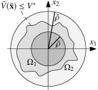
(a)

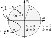
(b)

Figure 1: Example of sets (a) and time instants (b) described in the proof of Proposition 7 with $n=1$, $N=2$.

Note that, given the hypotheses of this Proposition, Lemma 11 (see Appendix) holds. Then, consider the set $\Omega_{1}\triangleq\{\bar{\mathbf{x}}\mid\left\lVert\bar{\mathbf{x}}\right\rVert\leq\bar{\rho}\}$, which is compact and where $\bar{\rho}$ is given by the Lemma. Since $\bar{V}$ is continuous and radially unbounded, we can find a scalar $V^{*}>0$ such that the compact set $\Omega_{2}\triangleq\{\bar{\mathbf{x}}\mid\bar{V}(\bar{\mathbf{x}})\leq V^{*}\}$ fulfils $\Omega_{2}\supset\Omega_{1}$. As $\Omega_{2}$ is compact, there exists a closed ball of the origin with radius $\tilde{\rho}\geq\bar{\rho}$ that contains $\Omega_{2}$; see the sketch diagram reported in Fig. 1a for the case that $n=1$, $N=2$. Now, we define the functions

$$\widetilde{V}(\bar{\mathbf{x}})\triangleq\begin{dcases}0,&\text{if }\left\lVert\bar{\mathbf{x}}\right\rVert\leq\tilde{\rho},\\ \bar{V}(\bar{\mathbf{x}}),&\text{otherwise},\end{dcases}$$ (10)

$$\tilde{\alpha}(\left\lVert\bar{\mathbf{x}}\right\rVert)\triangleq\begin{dcases}0,&\text{if }\left\lVert\bar{\mathbf{x}}\right\rVert\leq\tilde{\rho},\\ \bar{\alpha}(\left\lVert\bar{\mathbf{x}}\right\rVert),&\text{otherwise}.\end{dcases}$$ (11)

Next, we divide the generic time interval $[0,t]$ in $M-1$ contiguous sub-intervals $[t_{1}=0,t_{2}],\dots,[t_{M-1},t_{M}=t]$, where $t_{2}\dots,t_{M-1}$ are the time instants at which $\bar{\mathbf{x}}$ crosses transversely the level set where $\left\lVert\bar{\mathbf{x}}\right\rVert=\tilde{\rho}$ (see Fig. 1b). With this partition of the time interval $[0,t]$ we have that, in each sub-interval $[t_{j-1},t_{j}]$, either

$$\widetilde{V}(\bar{\mathbf{x}}(t_{j}))-\widetilde{V}(\bar{\mathbf{x}}(t_{j-1}))=0,$$ (12)

because of (10), or

$$\widetilde{V}(\bar{\mathbf{x}}(t_{j}))-\widetilde{V}(\bar{\mathbf{x}}(t_{j-1}))\leq\bar{p}(t_{j};\bar{\mathbf{x}}(t_{j-1})),$$ (13)

because of (9). Now, note that $\dot{\bar{p}}(\bar{\mathbf{x}})=-\bar{q}(\bar{\mathbf{x}})$; $\bar{q}$ being defined in Lemma 11. By exploiting the Lemma, with $\bar{\alpha}$ defined therein, we have

$$\dot{\bar{p}}(\bar{\mathbf{x}})=-\bar{q}(\bar{\mathbf{x}})\leq-\bar{\alpha}(\left\lVert\bar{\mathbf{x}}\right\rVert).$$ (14)

From (11) and (14), it follows that

$$\bar{p}(t_{j};\bar{\mathbf{x}}(t_{j-1}))\leq-\int_{t_{j-1}}^{t_{j}}\bar{\alpha}(\left\lVert\bar{\mathbf{x}}(\tau)\right\rVert)\mathrm{d}\tau=-\int_{t_{j-1}}^{t_{j}}\tilde{\alpha}(\left\lVert\bar{\mathbf{x}}(\tau)\right\rVert)\mathrm{d}\tau.$$ (15)

Combining (13) and (15), and from Lemma 11, we have

$$\widetilde{V}(\bar{\mathbf{x}}(t_{j}))-\widetilde{V}(\bar{\mathbf{x}}(t_{j-1}))\leq-\bar{p}(t_{j},\bar{\mathbf{x}}(t_{j-1}))\leq\\ -\int_{t_{j-1}}^{t_{j}}\tilde{\alpha}(\left\lVert\bar{\mathbf{x}}(\tau)\right\rVert)\ \mathrm{d}\tau\leq 0.$$ (16)

Therefore, since

$$\widetilde{V}(\bar{\mathbf{x}}(t))-\widetilde{V}(\bar{\mathbf{x}}(0))=[\widetilde{V}(\bar{\mathbf{x}}(t))-\widetilde{V}(\bar{\mathbf{x}}(t_{M-1}))]+[\widetilde{V}(\bar{\mathbf{x}}(t_{M-1}))\\ -\widetilde{V}(\bar{\mathbf{x}}(t_{M-2}))]+\ldots+[\widetilde{V}(\bar{\mathbf{x}}(t_{2}))-\widetilde{V}(\bar{\mathbf{x}}(0))],$$ (17)

exploiting (11), (12) and (16), we get

$$\widetilde{V}(\bar{\mathbf{x}}(t))-\widetilde{V}(\bar{\mathbf{x}}(0))\leq-\int_{0}^{t}\tilde{\alpha}(\left\lVert\bar{\mathbf{x}}(\tau)\right\rVert)\ \mathrm{d}\tau\leq 0.$$ (18)

Hence, $\widetilde{V}(\bar{\mathbf{x}}(t))\leq\widetilde{V}(\bar{\mathbf{x}}(0))$, i.e. $\widetilde{V}(\bar{\mathbf{x}}(t))$ is bounded for all $t\geq 0$. Also, for large values of $\bar{\mathbf{x}}$ ($\left\lVert\bar{\mathbf{x}}\right\rVert>\tilde{\rho}$), from (10) we have $\widetilde{V}(\bar{\mathbf{x}})=\bar{V}(\bar{\mathbf{x}})$; therefore $\widetilde{V}(\bar{\mathbf{x}})$ is radially unbounded as $\bar{V}(\bar{\mathbf{x}})$ is. Thus, $\widetilde{V}(\bar{\mathbf{x}}(t))$ being bounded implies that $\bar{\mathbf{x}}$ must be bounded (even if $\widetilde{V}$ is a discontinuous function). This means that network (1)-(2) is Lagrange stable, i.e. $\left\lVert\mathbf{x}(t)\right\rVert<+\infty$ for all $t$.

Next, we show that (1)-(2) is uniformly asymptotically bounded. We define

$$\tilde{\alpha}^{\prime}(\left\lVert\bar{\mathbf{x}}\right\rVert)\triangleq\begin{dcases}0,&\text{if }\left\lVert\bar{\mathbf{x}}\right\rVert\leq\tilde{\rho},\\ \bar{\alpha}(\left\lVert\bar{\mathbf{x}}\right\rVert)-\bar{\alpha}(\tilde{\rho}),&\text{otherwise},\end{dcases}$$ (19)

which is continuous and null if and only if $\left\lVert\bar{\mathbf{x}}\right\rVert\leq\tilde{\rho}$, as $\bar{\alpha}$ is increasing. In addition, since the network solutions are bounded, $\bar{\mathbf{x}}(t)$ belongs to a compact set, and therefore $\tilde{\alpha}^{\prime}(\left\lVert\bar{\mathbf{x}}(t)\right\rVert)$ is uniformly continuous in that set. From (18), we know that $\int_{0}^{t}\tilde{\alpha}(\left\lVert\bar{\mathbf{x}}(\tau)\right\rVert)\mathrm{d}\tau$ is finite for all $t\in[0,+\infty]$ as it is bounded by two finite terms. Consequently, $\int_{0}^{t}\tilde{\alpha}^{\prime}(\left\lVert\bar{\mathbf{x}}(\tau)\right\rVert)\mathrm{d}\tau$ is also bounded, and we can employ Lemma 3 to conclude that $\lim_{t\rightarrow+\infty}\tilde{\alpha}^{\prime}(\left\lVert\bar{\mathbf{x}}(t)\right\rVert)=0$. Since $\tilde{\alpha}^{\prime}(\left\lVert\bar{\mathbf{x}}\right\rVert)$ is null only when $\left\lVert\bar{\mathbf{x}}\right\rVert\leq\tilde{\rho}$, this means that

$$\mathop{\lim\sup}_{t\rightarrow+\infty}\left\lVert\bar{\mathbf{x}}(t)\right\rVert\leq\tilde{\rho}.$$ (20)

∎

IV Asymptotic convergence of heterogeneous networks

Before giving our main result, we define the average vector field $\tilde{\mathbf{f}}:\mathbb{R}^{nN}\rightarrow\mathbb{R}^{n}$ as follows:

$$\tilde{\mathbf{f}}(\bar{\mathbf{x}})\triangleq\frac{1}{N}\sum_{i=1}^{N}\mathbf{f}_{i}({\mathbf{x}_{i}})=\dot{\tilde{\mathbf{x}}},$$ (21)

where the coupling terms in $\dot{\tilde{\mathbf{x}}}$ cancel out since $\mathbf{L},\mathbf{L}_{\mathrm{d}}$ are symmetric. Recalling that $\mathbf{e}_{i}\triangleq\mathbf{x}_{i}-\tilde{\mathbf{x}}$, we can write

$$\dot{\mathbf{e}}_{i}=\dot{\mathbf{x}}_{i}-\dot{\tilde{\mathbf{x}}} =\mathbf{f}_{i}(\mathbf{x}_{i})-c\sum_{j=1}^{N}L_{ij}\bm{\Gamma}(\mathbf{x}_{j}-\mathbf{x}_{i})$$ (22)

$$-c_{\mathrm{d}}\sum_{j=1}^{N}L_{ij}^{\mathrm{d}}\bm{\Gamma}_{\mathrm{d}}\mathrm{sign}(\mathbf{x}_{j}-\mathbf{x}_{i})-\tilde{\mathbf{f}}(\bar{\mathbf{x}}).$$

Theorem 8.

Consider network (1) controlled by the distributed control action (2). If

1. the controlled network is uniformly ultimately bounded to the ball $\mathcal{B}_{r}^{\mathrm{c}}$, for some $r>0$;

2. each agent dynamics $\mathbf{f}_{i}$ is QUAD($\mathbf{P}$, $\mathbf{Q}_{i}$) in $\mathcal{B}_{r}^{\mathrm{c}}$, and $\mathrm{sym}(\mathbf{P}\bm{\Gamma})>0$, $\mu_{\infty}^{-}(\mathbf{P}\bm{\Gamma}_{\mathrm{d}})>0$;

3. $\mathcal{G}$ and $\mathcal{G}_{\mathrm{d}}$ are connected graphs;

then

1. there exist $c^{*}$ and $c_{\mathrm{d}}^{*}$ such that, if $c>c^{*}$ and $c_{\mathrm{d}}\geq c_{\mathrm{d}}^{*}$, then global asymptotic synchronization is achieved. Moreover, the asymptotic synchronous trajectory $\mathbf{s}(t)$ is a solution to $\dot{\mathbf{s}}(t)=\frac{1}{N}\sum_{i=1}^{N}\mathbf{f}_{i}(\mathbf{s}(t))$;

2. $c^{*}$ and $c_{\mathrm{d}}^{*}$ are given by

   $$c^{*}\triangleq\frac{\max_{i}{\left(\lVert\mathbf{Q}_{i}\rVert_{2}\right)}}{\lambda_{2}(\mathbf{L})\lambda_{\mathrm{min}}(\mathrm{sym}\ \mathbf{P}\bm{\Gamma})},\quad c^{*}_{\mathrm{d}}\triangleq\frac{\left\lVert\left(\left\lvert\mathbf{P}\right\rvert\right)\mathbf{m}\right\rVert_{\infty}}{\delta_{\mathcal{G}_{\mathrm{d}}}\mu_{\infty}^{-}(\mathbf{P}\bm{\Gamma}_{\mathrm{d}})},$$ (23)

   where $\delta_{\mathcal{G}_{\mathrm{d}}}$ is the minimum density [25] of the graph $\mathcal{G}_{\mathrm{d}}$, and $\mathbf{m}\in\mathbb{R}_{\geq 0}^{n}$ is a vector such that

   $$\mathbf{m}\geq\left\lvert\mathbf{f}_{i}(\tilde{\mathbf{x}})-\tilde{\mathbf{f}}(\bar{\mathbf{x}})\right\rvert,\quad\forall i\in\{1,\dots,N\},\ \forall\bar{\mathbf{x}}\in\mathcal{B}_{r}^{\mathrm{c}}.$$ (24)

Proof.

Consider the candidate common Lyapunov function $V\triangleq\frac{1}{2}\sum_{i=1}^{N}\mathbf{e}_{i}^{\mathsf{T}}\mathbf{P}\mathbf{e}_{i}.$ From (22), we have

$$\dot{V} =\sum_{i=1}^{N}\mathbf{e}_{i}^{\mathsf{T}}\mathbf{P}\left(\mathbf{f}_{i}(\mathbf{x}_{i})-\tilde{\mathbf{f}}(\bar{\mathbf{x}})\right)-c\sum_{i=1}^{N}\sum_{j=1}^{N}L_{ij}\mathbf{e}_{i}^{\mathsf{T}}\mathbf{P}\bm{\Gamma}\mathbf{e}_{j}$$ (25)

$$\phantom{=\,}-c_{\mathrm{d}}\sum_{i=1}^{N}\sum_{j=1}^{N}L_{ij}^{\mathrm{d}}\mathbf{e}_{i}^{\mathsf{T}}\mathbf{P}\bm{\Gamma}_{\mathrm{d}}\mathrm{sign}(\mathbf{e}_{j}-\mathbf{e}_{i}),$$

where we used the fact that $\mathrm{sign}(\mathbf{x}_{j}-\mathbf{x}_{i})=\mathrm{sign}(\mathbf{e}_{j}-\mathbf{e}_{i})$. Then, adding and subtracting $\sum_{i=1}^{N}\mathbf{e}_{i}^{\mathsf{T}}\mathbf{P}\mathbf{f}_{i}(\tilde{\mathbf{x}})$, we have

$$\dot{V}=\sum_{i=1}^{N}\mathbf{e}_{i}^{\mathsf{T}}\mathbf{P}\left(\mathbf{f}_{i}(\mathbf{x}_{i})-\mathbf{f}_{i}(\tilde{\mathbf{x}})\right)+\sum_{i=1}^{N}\mathbf{e}_{i}^{\mathsf{T}}\mathbf{P}\left(\mathbf{f}_{i}(\tilde{\mathbf{x}})-\tilde{\mathbf{f}}(\bar{\mathbf{x}})\right)\\ -c\sum_{i=1}^{N}\sum_{j=1}^{N}L_{ij}\mathbf{e}_{i}^{\mathsf{T}}\mathbf{P}\bm{\Gamma}\mathbf{e}_{j}-c_{\mathrm{d}}\sum_{i=1}^{N}\sum_{j=1}^{N}L_{ij}^{\mathrm{d}}\mathbf{e}_{i}^{\mathsf{T}}\mathbf{P}\bm{\Gamma}_{\mathrm{d}}\mathrm{sign}(\mathbf{e}_{j}-\mathbf{e}_{i}).$$

In addition, since the communication graphs are undirected ($L_{ij}^{\mathrm{d}}=L_{ji}^{\mathrm{d}}$), for each term $\mathbf{e}_{i}^{\mathsf{T}}\mathbf{P}\bm{\Gamma}_{\mathrm{d}}\mathrm{sign}(\mathbf{e}_{j}-\mathbf{e}_{i})$, there must exist the symmetric term $\mathbf{e}_{j}^{\mathsf{T}}\mathbf{P}\bm{\Gamma}_{\mathrm{d}}\mathrm{sign}(\mathbf{e}_{i}-\mathbf{e}_{j})$. Hence, we may recast $\dot{V}$ as

$$\dot{V}=\sum_{i=1}^{N}\mathbf{e}_{i}^{\mathsf{T}}\mathbf{P}\left(\mathbf{f}_{i}(\mathbf{x}_{i})-\mathbf{f}_{i}(\tilde{\mathbf{x}})\right)+\sum_{i=1}^{N}\mathbf{e}_{i}^{\mathsf{T}}\mathbf{P}\left(\mathbf{f}_{i}(\tilde{\mathbf{x}})-\tilde{\mathbf{f}}(\bar{\mathbf{x}})\right)\\ -c\sum_{i=1}^{N}\sum_{j=1}^{N}L_{ij}\mathbf{e}_{i}^{\mathsf{T}}\mathbf{P}\bm{\Gamma}\mathbf{e}_{j}-c_{\mathrm{d}}\sum_{(i,j)\in\mathcal{E}_{\mathrm{d}}}(\mathbf{e}_{i}-\mathbf{e}_{j})^{\mathsf{T}}\mathbf{P}\bm{\Gamma}_{\mathrm{d}}\mathrm{sign}(\mathbf{e}_{i}-\mathbf{e}_{j}).$$

As the network is uniformly ultimately bounded, there exists a finite $T^{*}>0$ such that, for $t\geq T^{*}$, $\left\lVert\mathbf{x}(t)\right\rVert\in\mathcal{B}_{r}^{\mathrm{c}}$. From now on, we take $t\geq T^{*}$, and, since $\mathbf{f}_{i}$ is QUAD($\mathbf{P}$, $\mathbf{Q}_{i}$), we get

$$\dot{V}\leq\sum_{i=1}^{N}\left(\mathbf{e}_{i}^{\mathsf{T}}\mathbf{Q}_{i}\mathbf{e}_{i}\right)+\sum_{i=1}^{N}\mathbf{e}_{i}^{\mathsf{T}}\mathbf{P}\left(\mathbf{f}_{i}(\tilde{\mathbf{x}})-\tilde{\mathbf{f}}(\bar{\mathbf{x}})\right)-c\sum_{i=1}^{N}\sum_{j=1}^{N}L_{ij}\\ \mathbf{e}_{i}^{\mathsf{T}}\mathbf{P}\bm{\Gamma}\mathbf{e}_{j}-c_{\mathrm{d}}\sum_{(i,j)\in\mathcal{E}_{\mathrm{d}}}(\mathbf{e}_{i}-\mathbf{e}_{j})^{\mathsf{T}}\mathbf{P}\bm{\Gamma}_{\mathrm{d}}\mathrm{sign}(\mathbf{e}_{i}-\mathbf{e}_{j}).$$ (26)

By defining the diagonal block matrix $\bar{\mathbf{Q}}$ having $\mathbf{Q}_{1},\dots,\mathbf{Q}_{N}$ on its diagonal, we can write $\sum_{i=1}^{N}\left(\mathbf{e}_{i}^{\mathsf{T}}\mathbf{Q}_{i}\mathbf{e}_{i}\right)=\bar{\mathbf{e}}^{\mathsf{T}}\bar{\mathbf{Q}}\bar{\mathbf{e}}$.

As all $\mathbf{f}_{i}$’s are QUAD in $\mathcal{B}_{r}^{\mathrm{c}}$, they are also bounded therein. Then, there exists a vector $\mathbf{m}\in\mathbb{R}^{n}_{\geq 0}$, such that

$$\mathbf{m}\geq\left\lvert\mathbf{f}_{i}(\tilde{\mathbf{x}})-\tilde{\mathbf{f}}(\bar{\mathbf{x}})\right\rvert,\qquad\forall i\in\{1,\dots,N\},\ \forall\bar{\mathbf{x}}\in\mathcal{B}_{r}^{\mathrm{c}}.$$ (27)

Therefore, letting $M\triangleq\left\lVert\left(\left\lvert\mathbf{P}\right\rvert\right)\mathbf{m}\right\rVert_{\infty}$, it holds that

$$\sum_{i=1}^{N}\mathbf{e}_{i}^{\mathsf{T}}\mathbf{P}\left(\mathbf{f}_{i}(\tilde{\mathbf{x}})-\tilde{\mathbf{f}}(\bar{\mathbf{x}})\right) \leq\sum_{i=1}^{N}\left\lVert\mathbf{e}_{i}\right\rVert_{1}\left\lVert\mathbf{P}\left(\mathbf{f}_{i}(\tilde{\mathbf{x}})-\tilde{\mathbf{f}}(\bar{\mathbf{x}})\right)\right\rVert_{\infty}$$ (28)

$$\leq M\sum_{i=1}^{N}\left\lVert\mathbf{e}_{i}\right\rVert_{1}=M\left\lVert\bar{\mathbf{e}}\right\rVert_{1}.$$

Defining $\bar{\mathbf{a}}\triangleq\left(\mathbf{B}_{\mathrm{d}}^{\mathsf{T}}\otimes\mathbf{I}_{n}\right)\bar{\mathbf{e}}$, we obtain $\dot{V}\leq W_{1}+W_{2}$, where

$$W_{1} \triangleq\bar{\mathbf{e}}^{\mathsf{T}}\left(\bar{\mathbf{Q}}-c\mathbf{L}\otimes\mathbf{P}\bm{\Gamma}\right)\bar{\mathbf{e}},$$ (29)

$$W_{2} \triangleq M\left\lVert\bar{\mathbf{e}}\right\rVert_{1}-c_{\mathrm{d}}\bar{\mathbf{a}}^{\mathsf{T}}\left(\mathbf{I}_{N_{\mathcal{E}_{\mathrm{d}}}}\otimes\mathbf{P}\bm{\Gamma}_{\mathrm{d}}\right)\mathrm{sign}(\bar{\mathbf{a}}).$$ (30)

Then, following the steps in [25, proof of Theorem 5], we find that $W_{1}<0$ if $c>c^{*}$, and $W_{2}\leq 0$ if $c_{\mathrm{d}}\geq c_{\mathrm{d}}^{*}$, with $c^{*},c_{\mathrm{d}}^{*}$ given by (23). Finally, since $W_{1}<0$ and $W_{2}\leq 0$, then $\dot{V}<0$, which means that all $\mathbf{e}_{i}$’s tend to zero, i.e. all $\mathbf{x}_{i}$’s tend to $\tilde{\mathbf{x}}$, whose dynamics is given in (21). ∎

Remark 9.

Note that the assumptions on boundedness and QUADness in Theorem 8 are quite mild and they can be easily verified. Indeed, uniform ultimate boundedness of network (1) can be checked by using Proposition 7, while the QUADness hypothesis on the dynamics can be verified by testing boundedness of the Jacobian of the individual vector fields; see Proposition 12.

Remark 10.

Theorem 8 can be easily adapted to account for possible discontinuities in the nodes’ dynamics. In that case, the agents must be -QUAD($\mathbf{P}$, $\mathbf{Q}_{i}$, $\mathbf{M}_{i}$) [25] (rather than QUAD) and the critical threshold for the discontinuous coupling layer can be proved to be

$$c^{*}_{\mathrm{d}}\triangleq\frac{\left\lVert\left(\left\lvert\mathbf{P}\right\rvert\right)\mathbf{m}\right\rVert_{\infty}+\left\lVert\bar{\mathbf{M}}\right\rVert_{\infty}}{\delta_{\mathcal{G}_{\mathrm{d}}}\mu_{\infty}^{-}(\mathbf{P}\bm{\Gamma}_{\mathrm{d}})},\quad\bar{\mathbf{M}}\triangleq\begin{bmatrix}\mathbf{M}_{1}&&\\ &\ddots&\\ &&\mathbf{M}_{N}\end{bmatrix}.$$ (31)

V Numerical validation

We consider a set of 3 modified van der Pol oscillators of the form

$$\dot{\mathbf{x}}=\mathbf{f}_{i}(\mathbf{x})+\mathbf{u}=\begin{bmatrix}x_{1}-\epsilon x_{1}\\ \mu_{i}(1-x_{1}^{2}-\eta x_{2}^{2})x_{2}-x_{1}\\ \end{bmatrix}+\begin{bmatrix}u_{1}\\ u_{2}\end{bmatrix},$$ (32)

for $i=1,2,3$, with $\epsilon=0.01$, $\eta=0.001$, and $\mu_{1}=1$, $\mu_{2}=2$, $\mu_{3}=3$. We couple the agents through the diffusive and discontinuous coupling law (2), with $\mathbf{L}$, $\mathbf{L}_{\mathrm{d}}$ corresponding to complete graphs, and $\bm{\Gamma}=\bm{\Gamma}_{\mathrm{d}}=\mathbf{I}_{2}$. Introducing the storage function $V_{i}(\mathbf{x})=\frac{1}{2}(x_{1}^{2}+x_{2}^{2})$, we can show systems (32) are strongly strictly semipassive. Indeed,

$$\begin{split}\dot{V}_{i}&=x_{1}\dot{x}_{1}+x_{2}\dot{x}_{2}\\ &=x_{1}x_{2}-\epsilon x_{1}^{2}+x_{1}u_{1}+\mu_{i}x_{2}^{2}(1-x_{1}^{2}-\eta x_{2}^{2})-x_{1}x_{2}+x_{2}u_{2}\\ &=-\epsilon x_{1}^{2}+\mu_{i}x_{2}^{2}(1-x_{1}^{2}-\eta x_{2}^{2})+\mathbf{x}^{\mathsf{T}}\mathbf{u}=-h_{i}(\mathbf{x})+\mathbf{y}^{\mathsf{T}}\mathbf{u},\end{split}$$

where $h_{i}(\mathbf{x})\triangleq\epsilon x_{1}^{2}+\mu_{i}x_{2}^{2}(x_{1}^{2}+\eta x_{2}^{2}-1)$. From Proposition 7, it follows that the network is uniformly ultimately bounded to $\mathcal{B}_{r}^{\mathrm{c}}$ for some $r$; a numerical exploration shows that $r=7.72$ is a suitable value. Since $\mathbf{f}$ is continuous, its Jacobian is bounded in $\mathcal{B}_{r}^{\mathrm{c}}$, and the three agents are QUAD($\mathbf{I}$, $\mathbf{Q}_{i}$), $i=1,2,3$ (see Proposition 12 in the Appendix), All the assumptions of Theorem 8 are fulfilled, and its thesis can be used to compute the critical values $c^{*}$ and $c_{\mathrm{d}}^{*}$ that guarantee asymptotic synchronization. Specifically, knowing $r$, we can compute analytically that $\max_{i}{\left(\lVert\mathbf{Q}_{i}\rVert_{2}\right)}\approx 11.58$, and numerically that $\left\lVert\mathbf{m}\right\rVert_{\infty}\approx 179.90$; moreover, $\lambda_{2}(\mathbf{L})=N=3$, and $\delta_{\mathcal{G}_{\mathrm{d}}}=N/2=3/2$ [25]. Therefore, through (23), we compute that $c^{*}=3.86$ and $c_{\mathrm{d}}^{*}=119.93$.

In Fig. 2, two simulations are reported. Namely, in Fig. 2a, where $c=4>c^{*}$ and the discontinuous coupling is absent, the network does not achieve synchronization. When the discontinuous action is turned on with strength $c_{\mathrm{d}}=120>c_{\mathrm{d}}^{*}$ in Fig. 2b, convergence is attained. Note that even if $c$ were larger, the diffusive coupling alone would not be able to bring the synchronization error to zero (simulations omitted here for the sake of brevity). Also, the analytical thresholds $c^{*}$, $c_{\mathrm{d}}^{*}$ are conservative.

VI Conclusions

This paper solves the problem of achieving asymptotic convergence in networks of heterogeneous nonlinear systems. In particular, a distributed approach is proposed that combines traditional diffusive coupling with a discontinuous coupling layer that, under suitable assumptions on the individual dynamics, is capable of guaranteeing asymptotic convergence of all the nodes towards a common trajectory. To support the control design, we provided analytical estimates of the minimum coupling gains required to achieve complete synchronization, as a function of the node dynamics, and of the topology of the diffusive and discontinuous layers. The effectiveness of the approach was demonstrated via a representative example.

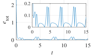
(a)

(b)

Figure 2: Total synchronization error $e_{\mathrm{tot}}\triangleq\frac{1}{N}\sum_{i=1}^{N}\left\lVert\mathbf{e}_{i}\right\rVert_{2}$ in a network of three different modified van der Pol oscillators (32). In (a), $c=4$, $c_{\mathrm{d}}=0$; in (b), $c=4$, $c_{\mathrm{d}}=120$. The initial conditions are $\bar{\mathbf{x}}(t=0)=[1.5\ \ 1.5\ \ 1.75\ \ 1.75\ \ 2\ \ 2]^{\mathsf{T}}$.

Lemma 11.

Consider network (1)-(2). If

1. all systems in (1) are strongly strictly semipassive, with stability components $h_{i}$, $i=1,\dots,N$;

2. $c\geq 0$, $c_{\mathrm{d}}\geq 0$, $\mathrm{sym}(\bm{\Gamma})\geq 0$, and $\mu_{\infty}^{-}(\bm{\Gamma}_{\mathrm{d}})\geq 0$;

then there exists a finite $\bar{\rho}\geq 0$ such that

$$\bar{q}(\bar{\mathbf{x}})\triangleq\sum_{i=1}^{N}\left(h_{i}(\mathbf{x}_{i})-\mathbf{y}_{i}^{\mathsf{T}}\mathbf{u}_{i}\right)\geq\bar{\alpha}(\left\lVert\bar{\mathbf{x}}\right\rVert),\quad\text{if }\left\lVert\bar{\mathbf{x}}\right\rVert\geq\bar{\rho},$$ (33)

where $\bar{\alpha}:{}[\bar{\rho},+\infty[{}\rightarrow\mathbb{R}_{\geq 0}$ is a continuous and increasing scalar function.

Proof.

First, it is straightforward to verify that

$$-\sum_{i=1}^{N}\mathbf{y}_{i}^{\mathsf{T}}\mathbf{u}_{i}=\bar{\mathbf{y}}^{\mathsf{T}}\bar{\mathbf{u}}=\bar{\mathbf{x}}^{\mathsf{T}}\bar{\mathbf{u}}=\\ c\bar{\mathbf{x}}^{\mathsf{T}}(\mathbf{L}\otimes\bm{\Gamma})\bar{\mathbf{x}}+c_{\mathrm{d}}\bar{\mathbf{z}}^{\mathsf{T}}(\mathbf{I}_{N_{\mathcal{E}_{\mathrm{d}}}}\otimes\bm{\Gamma}_{\mathrm{d}})\mathrm{sign}(\bar{\mathbf{z}}),$$ (34)

where $N_{\mathcal{E}_{\mathrm{d}}}$ is the number of edges in $\mathcal{G}_{\mathrm{d}}$, and $\bar{\mathbf{z}}\triangleq(\mathbf{B}_{\mathrm{d}}^{\mathsf{T}}\otimes\mathbf{I}_{n})\bar{\mathbf{x}}$, with $\mathbf{B}_{\mathrm{d}}$ being the incidence matrix of $\mathcal{G}_{\mathrm{d}}$. Simple algebraic manipulations show that the first term on the right-hand side of (34) is non-negative as $c\geq 0$ and $\mathrm{sym}(\bm{\Gamma})\geq 0$. By exploiting [25, Lemma 9], we can also conclude that the second term is non-negative as $c_{\mathrm{d}}\geq 0$ and $\mu_{\infty}^{-}(\bm{\Gamma}_{\mathrm{d}})\geq 0$. To complete the proof, we need to find a scalar $\bar{\rho}$ such that, if $\left\lVert\bar{\mathbf{x}}\right\rVert>\bar{\rho}$, it holds that $\sum_{i=1}^{N}h_{i}(\mathbf{x}_{i})\geq\bar{\alpha}(\left\lVert\bar{\mathbf{x}}\right\rVert).$ Such a scalar can be found as follows. Firstly, note that:

• for any $i\in\{1,\dots,N\}$, as $h_{i}$ is continuous, it is also bounded in the set $\{\mathbf{x}_{i}\in\mathbb{R}^{n}\mid\left\lVert\mathbf{x}_{i}\right\rVert\leq\rho_{i}\}$, therefore there exists a finte scalar $H_{i}\leq 0$ such that $h_{i}(\mathbf{x}_{i})\geq H_{i}$ in that set. In addition, $h_{i}$ is non-negative by definition in $\{\mathbf{x}_{i}\in\mathbb{R}^{n}\mid\left\lVert\mathbf{x}_{i}\right\rVert\geq\rho_{i}\}$; hence,

  $$h_{i}(\mathbf{x}_{i})\geq H_{i},\quad\forall\mathbf{x}_{i}\in\mathbb{R}^{n};$$ (35)

• as all systems are strongly strictly semipassive, for each stability component $h_{i}$ there exists an increasing and radially unbounded function $\alpha_{i}$ associated to it. This implies that, for a given $i\in\{1,\dots,N\}$ and scalar $b$, there exists another scalar $a\geq\rho_{i}$ such that

  $$\alpha_{i}(\left\lVert\mathbf{x}_{i}\right\rVert)>b,\quad\text{if }\left\lVert\mathbf{x}_{i}\right\rVert>a.$$ (36)

From (36), there exist $N$ scalars $\rho_{i}^{\prime}\geq\rho_{i}$, for $i=1,\dots,N$, such that

$$\alpha_{i}(\left\lVert\mathbf{x}_{i}\right\rVert)>-\sum_{\begin{subarray}{c}j=1,j\neq i\end{subarray}}^{N}H_{j},\quad\text{if }\left\lVert\mathbf{x}_{i}\right\rVert>\rho_{i}^{\prime}.$$ (37)

Now, define the following partition of $\{1,\dots,N\}$, whose sets are $\mathcal{I}_{1}\triangleq\{i\mid\left\lVert\mathbf{x}_{i}\right\rVert\leq\rho_{i}\}$, $\mathcal{I}_{2}\triangleq\{i\mid\rho_{i}<\left\lVert\mathbf{x}_{i}\right\rVert\leq\rho_{i}^{\prime}\}$, and $\mathcal{I}_{3}\triangleq\{i\mid\left\lVert\mathbf{x}_{i}\right\rVert>\rho_{i}^{\prime}\}$. Then, it is possible to write $\sum_{i=1}^{N}h_{i}(\mathbf{x}_{i})=\sum_{i\in\mathcal{I}_{1}\cup\mathcal{I}_{2}\cup\mathcal{I}_{3}}h_{i}(\mathbf{x}_{i})$. Exploiting (35), we get $\sum_{i=1}^{N}h_{i}(\mathbf{x}_{i})\geq\sum_{i\in\mathcal{I}_{1}}H_{i}+\sum_{i\in\mathcal{I}_{2}\cup\mathcal{I}_{3}}h_{i}(\mathbf{x}_{i});$ applying (6), we have $\sum_{i=1}^{N}h_{i}(\mathbf{x}_{i})\geq\sum_{i\in\mathcal{I}_{1}}H_{i}+\sum_{i\in\mathcal{I}_{2}\cup\mathcal{I}_{3}}\alpha_{i}(\left\lVert\mathbf{x}_{i}\right\rVert)$. Then, we define $\bar{\rho}\triangleq\sqrt{\sum_{i=1}^{N}(\rho_{i}^{\prime})^{2}}$, so that

$$\left\lVert\bar{\mathbf{x}}\right\rVert>\bar{\rho}\ \ \Rightarrow\ \ \exists i:\left\lVert\mathbf{x}_{i}\right\rVert>\rho_{i}^{\prime}\ \ \Leftrightarrow\ \ \mathcal{I}_{3}\neq\varnothing.$$ (38)

For all $\left\lVert\bar{\mathbf{x}}\right\rVert>\bar{\rho}$, we can exploit (37) and (38) to write that

$$\sum_{i=1}^{N}h_{i}(\mathbf{x}_{i})\geq\sum_{i\in\mathcal{I}_{1}}H_{i}+\sum_{i\in\mathcal{I}_{2}\cup\mathcal{I}_{3}}\alpha_{i}(\left\lVert\mathbf{x}_{i}\right\rVert)>0.$$ (39)

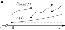
Figure 3: Example of the functions $\bar{\alpha}_{\mathrm{bound}}$ and $\bar{\alpha}$ in the proof of Lemma 11.

At this point, we define the (not necessarily continuous) positive function $\bar{\alpha}_{\mathrm{bound}}:{}]\bar{\rho},+\infty[{}\rightarrow\mathbb{R}_{>0}$ given by

$$\bar{\alpha}_{\mathrm{bound}}(s)\triangleq\min_{\bar{\mathbf{x}}:\left\lVert\bar{\mathbf{x}}\right\rVert=s}\left(\sum_{i\in\mathcal{I}_{1}}H_{i}+\sum_{i\in\mathcal{I}_{2}\cup\mathcal{I}_{3}}\alpha_{i}(\left\lVert\mathbf{x}_{i}\right\rVert)\right)>0.$$

Then, we can define a continuous increasing function $\bar{\alpha}:{}[\bar{\rho},+\infty[{}\rightarrow\mathbb{R}_{\geq 0}$ that satisfies

(i) $$\qquad 0<\bar{\alpha}(s)\leq\bar{\alpha}_{\mathrm{bound}}(s),\quad\text{if }s>\bar{\rho},$$ (40)

(ii) $$\phantom{\qquad 0<{}}\bar{\alpha}(\bar{\rho})=\lim_{s\searrow\bar{\rho}}\bar{\alpha}(s);$$

see Fig. 3 for an illustration of $\bar{\alpha}$ and $\bar{\alpha}_{\mathrm{bound}}$. From (39),

$$\sum_{i=1}^{N}h_{i}(\mathbf{x}_{i})\geq\bar{\alpha}(\left\lVert\bar{\mathbf{x}}\right\rVert),\quad\text{if }\left\lVert\bar{\mathbf{x}}\right\rVert\geq\bar{\rho},$$ (41)

which, since (34) is non-negative, proves the Lemma.∎

Proposition 12.

If a function $\mathbf{f}:\mathbb{R}^{n}\rightarrow\mathbb{R}^{n}$ has an upper bounded Jacobian in $\Omega\subseteq\mathbb{R}^{n}$, in the sense that for all $\mathbf{x}\in\Omega$

$${\partial f_{i}(\mathbf{x})}/{\partial x_{i}}\leq S_{ii},\qquad\left\lvert{\partial f_{i}(\mathbf{x})}/{\partial x_{j}}\right\rvert\leq S_{ij},\ i\neq j,$$ (42)

for $S_{ij}\in\mathbb{R}_{\geq 0}$, $i,j=1,\dots,n$, then $\mathbf{f}$ is QUAD($\mathbf{I}$, $\mathbf{Q}$) in $\Omega$, with $\mathbf{Q}$ being diagonal and $Q_{ii}=S_{ii}+\sum_{j=1,j\neq i}^{n}(S_{ij}+S_{ji})/{2}$.

Proof.

Let us define $\mathbf{x},\bm{\delta}\in\mathbb{R}^{n}$, so that $\mathbf{x},\mathbf{x}+\bm{\delta}\in\Omega$. From the mean value theorem, there exists $\lambda_{i}\in[0,1]$ such that $f_{i}(\mathbf{x}+\bm{\delta})-f_{i}(\mathbf{x})=\nabla f_{i}(\mathbf{x}+\lambda_{i}\bm{\delta})\ \bm{\delta}.$ This can be rewritten as $f_{i}(\mathbf{x}+\bm{\delta})-f_{i}(\mathbf{x})=\sum_{j=1}^{n}\hat{J}_{ij}\delta_{j},$ where $\hat{J}_{ij}={\partial f_{i}(\mathbf{x}+\lambda_{i}\bm{\delta})}/{\partial x_{j}}$, which, multiplying both sides by $\delta_{i}$, yields

$$\delta_{i}\cdot[f_{i}(\mathbf{x}+\bm{\delta})-f_{i}(\mathbf{x})]=\sum_{j=1}^{n}\hat{J}_{ij}\delta_{i}\delta_{j}.$$ (43)

Summing (43) for $i=1,\dots,n$, we have

$$\bm{\delta}^{\mathsf{T}}[\mathbf{f}(\mathbf{x}+\bm{\delta})-\mathbf{f}(\mathbf{x})]=\sum_{i=1}^{n}\hat{J}_{ii}\delta_{i}^{2}+\sum_{i=1}^{n}\sum_{j=1,j\neq i}^{n}\hat{J}_{ij}\delta_{i}\delta_{j}.$$ (44)

Recalling the expression of the square of a binomial and the bounds on the Jacobian, it holds that $\hat{J}_{ij}\delta_{i}\delta_{j}\leq\left\lvert\hat{J}_{ij}\delta_{i}\delta_{j}\right\rvert\leq\left\lvert\hat{J}_{ij}\right\rvert(\delta_{i}^{2}+\delta_{j}^{2})/2\leq S_{ij}(\delta_{i}^{2}+\delta_{j}^{2})/2.$ Then, letting $Q_{ii}=S_{ii}+\sum_{j=1,j\neq i}^{n}(S_{ij}+S_{ji})/2$, we have

$$\bm{\delta}^{\mathsf{T}}[\mathbf{f}(\mathbf{x}+\bm{\delta}-\mathbf{f}(\mathbf{x})]\leq\sum_{i=1}^{n}\hat{J}_{ii}\delta_{i}^{2}+\sum_{i=1}^{n}\sum_{j=1,j\neq i}^{n}\frac{S_{ij}}{2}\left(\delta_{i}^{2}+\delta_{j}^{2}\right)\\ \leq\sum_{i=1}^{n}S_{ii}\delta_{i}^{2}+\sum_{i=1}^{n}\sum_{j=1,j\neq i}^{n}\frac{S_{ij}}{2}\left(\delta_{i}^{2}+\delta_{j}^{2}\right)\leq\sum_{i=1}^{n}Q_{ii}\delta_{i}^{2}.$$ (45)

Defining $\mathbf{y}\triangleq\mathbf{x}+\bm{\delta}$, the thesis follows. ∎

References

- [1] Y. Tang, F. Qian, H. Gao, and J. Kurths, “Synchronization in complex networks and its application—a survey of recent advances and challenges,” Annu. Rev. Control, vol. 38, no. 2, pp. 184–198, 2014.
- [2] F. Dörfler and F. Bullo, “Synchronization in complex networks of phase oscillators: A survey,” Automatica, vol. 50, no. 6, pp. 1539–1564, 2014.
- [3] K.-K. Oh, M.-C. Park, and H.-S. Ahn, “A survey of multi-agent formation control,” Automatica, vol. 53, pp. 424–440, 2015.
- [4] D. J. Hill and J. Zhao, “Global synchronization of complex dynamical networks with non-identical nodes,” in 47th IEEE Conf. on Decision and Control, 2008, pp. 817–822.
- [5] W. He, W. Du, F. Qian, and J. Cao, “Synchronization analysis of heterogeneous dynamical networks,” Neurocomputing, vol. 104, pp. 146–154, 2013.
- [6] P. DeLellis, M. Di Bernardo, and D. Liuzza, “Convergence and synchronization in heterogeneous networks of smooth and piecewise smooth systems,” Automatica, vol. 56, pp. 1–11, 2015.
- [7] J. M. Montenbruck, M. Bürger, and F. Allgöwer, “Practical synchronization with diffusive couplings,” Automatica, vol. 53, pp. 235–243, 2015.
- [8] E. Panteley and A. Loría, “Synchronization and dynamic consensus of heterogeneous networked systems,” IEEE T. Automat. Contr., vol. 62, no. 8, pp. 3758–3773, 2017.
- [9] J. Xiang and G. Chen, “On the V-stability of complex dynamical networks,” Automatica, vol. 43, no. 6, pp. 1049–1057, 2007.
- [10] J. Zhao, D. J. Hill, and T. Liu, “Passivity-based output synchronization of dynamical networks with non-identical nodes,” in 49th IEEE Conf. on Decision and Control, 2010, pp. 7351–7356.
- [11] ——, “Stability of dynamical networks with non-identical nodes: A multiple V-Lyapunov function method,” Automatica, vol. 47, no. 12, pp. 2615–2625, 2011.
- [12] ——, “Synchronization of dynamical networks with nonidentical nodes: Criteria and control,” IEEE T. Circuits-I, vol. 58, no. 3, pp. 584–594, 2010.
- [13] Y. Wang and J. Cao, “Cluster synchronization in nonlinearly coupled delayed networks of non-identical dynamic systems,” Nonlinear Anal.-Real, vol. 14, no. 1, pp. 842–851, 2013.
- [14] D. M. Abrams and S. H. Strogatz, “Chimera states for coupled oscillators,” Physical review letters, vol. 93, no. 17, p. 174102, 2004.
- [15] C. R. Laing, “Chimera states in heterogeneous networks,” Chaos, vol. 19, no. 1, p. 013113, 2009.
- [16] G. S. Seyboth, D. V. Dimarogonas, K. H. Johansson, P. Frasca, and F. Allgöwer, “On robust synchronization of heterogeneous linear multi-agent systems with static couplings,” Automatica, vol. 53, pp. 392–399, 2015.
- [17] H. F. Grip, T. Yang, A. Saberi, and A. A. Stoorvogel, “Output synchronization for heterogeneous networks of non-introspective agents,” Automatica, vol. 48, no. 10, pp. 2444–2453, 2012.
- [18] N. Chopra and M. W. Spong, “Output synchronization of nonlinear systems with relative degree one,” in Recent advances in learning and control. Springer, 2008, pp. 51–64.
- [19] D. Lee, W. Yoo, D. Ji, and J. H. Park, “Integral control for synchronization of complex dynamical networks with unknown non-identical nodes,” Appl. Math. Comput., vol. 224, pp. 140–149, 2013.
- [20] X. Yang, Z. Wu, and J. Cao, “Finite-time synchronization of complex networks with nonidentical discontinuous nodes,” Nonlinear Dynam., vol. 73, no. 4, pp. 2313–2327, 2013.
- [21] D. A. Burbano, P. DeLellis et al., “Self-tuning proportional integral control for consensus in heterogeneous multi-agent systems,” Eur. J. Appl. Math., vol. 27, no. 6, pp. 923–940, 2016.
- [22] J. Cortés, “Finite-time convergent gradient flows with applications to network consensus,” Automatica, vol. 42, no. 11, pp. 1993–2000, 2006.
- [23] Q. Hui, W. M. Haddad, and S. P. Bhat, “Finite-time semistability, filippov systems, and consensus protocols for nonlinear dynamical networks with switching topologies,” Nonlinear Anal. Hybri., vol. 4, no. 3, pp. 557–573, 2010.
- [24] X. Liu, J. Lam, W. Yu, and G. Chen, “Finite-time consensus of multiagent systems with a switching protocol,” IEEE T. Neur. Net. Lear., vol. 27, no. 4, pp. 853–862, 2015.
- [25] M. Coraggio, P. DeLellis, and M. di Bernardo, “Achieving convergence and synchronization in networks of piecewise-smooth systems via distributed discontinuous coupling,” Submitted to Automatica (arxiv:1905.05863), 2019.
- [26] P. DeLellis, M. di Bernardo, and G. Russo, “On QUAD, Lipschitz, and contracting vector fields for consensus and synchronization of networks,” IEEE T. Circuits-I, vol. 58, no. 3, pp. 576–583, 2011.
- [27] J. A. Gallegos, M. A. Duarte-Mermoud, N. Aguila-Camacho, and R. Castro-Linares, “On fractional extensions of Barbalat lemma,” Syst. Control Lett., vol. 84, pp. 7–12, 2015.
- [28] A. Pogromsky, T. Glad, and H. Nijmeijer, “On diffusion driven oscillations in coupled dynamical systems,” Int. J. Bifurcat. Chaos, vol. 9, no. 04, pp. 629–644, 1999.
- [29] T. Nakakuki, T. Shen, and K. Tamura, “A remark on passivity of discontinuous systems,” IFAC Proc. Vol., vol. 39, no. 9, pp. 268–272, 2006.
- [30] J. Cortes, “Discontinuous dynamical systems,” IEEE Contr. Syst. Mag., vol. 28, no. 3, pp. 36–73, 2008.