Distributed Set-Based Observers Using Diffusion Strategies

Abstract

We propose two distributed set-based observers using strip-based and set-propagation approaches for linear discrete-time dynamical systems with bounded modeling and measurement uncertainties. Both algorithms utilize a set-based diffusion step, which decreases the estimation errors and the size of estimated sets, and can be seen as a lightweight approach to achieve partial consensus between the distributed estimated sets. Every node shares its measurement with its neighbor in the measurement update step. In the diffusion step, the neighbors intersect their estimated sets using our novel lightweight zonotope intersection technique. A localization example demonstrates the applicability of our algorithms.

1 Introduction

State estimation algorithms compute a single state, a probability distribution of the state, or a set of all possible states. In stochastic approaches, measurement and process noise are modeled by probability distributions (e.g., Gaussian [1]). On the other hand, set-based approaches assume noise to be unknown but bounded by known bounds. Safety-critical applications require guarantees on the state estimation during operation – such guarantees can be provided by set-based approaches. Set-based approaches are traditionally used in fault detection by generating an adaptive threshold to check the consistency of the measurements with the estimated output set [2, 3, 4, 5, 6]. According to the terminology in [7], there are three types of set-based observers: interval-based observers, set-propagation observers, and strip-based obser-vers. We focus on the following literature survey on set-propagation and strip-based observers as they are the paper’s main focus.

Set-propagation observers: They are based on a Luenberger observer and, in general, obtain possible sets of states by combining the model and the measurements through an observer gain [8]. By merging optimal and robust observer gain designs, a zonotopic Kalman filter (ZKF) is proposed in [9] based on the Frobenius norm of a zonotope. The same author proposed a joint zonotopic and Gaussian Kalman filter (ZGKF) in [10] along with robust fault detection in the presence of both bounded and Gaussian disturbances. This line of work has been extended to nonlinear systems using a zonotopic extended Kalman filter (ZEKF) in [11].

Strip-based observers: Unlike set-propagation observ-ers, which are based on observer gain derivation, strip-based observers generally intersect the set of states consistent with the model and the set consistent with the measurements to obtain the corrected state set [7]. One early example of strip-based observers is a recursive algorithm bounding the state by ellipsoids [12]. Another example based on normalized least-mean-squares is presented in [13]. A strip-based state estimation algorithm based on DC programming is proposed in [14]. Authors in [15] consider linear time-varying descriptor systems for strip-based estimation. Strip-baseds observers for nonlinear models are investigated in [16, 17, 18, 19, 20]. They are also used in applications such as underwater robotics [21], a leader following consensus problem in networked multi-agent systems [22], and localization [23]. Authors in [24] consider a class of discrete time-varying systems with an event-based communication mechanism over sensor networks. An interconnected multi-rate system is considered in [25]. A strip-based filtering subject to replay attacks and quantization effects is considered in [26] and [27], respectively. Also, a distributed strip-based estimation and formation control algorithm for a fleet of vehicles is proposed in [28], where the set-based estimation enclosure is guaranteed in spite of the lack of knowledge of the control signal applied by the rest of the vehicles.

Different set representations have been used in set-based estimation, e.g., ellipsoids [29, 30, 31], orthotopes, and polytopes [32, 33]. Zonotopes [34] are a special class of polytopes for which one can efficiently compute linear maps and Minkowski sums – both are important operations for set-based observers. A strip-based observer based on zonotopes is introduced in [35]. Another strip-based approach for disc-rete-time piecewise affine systems using zonotopes is studied in [36]. Yet another work considers discrete-time descriptor systems using zonotopes [37]. Set-based estimation of uncertain discrete-time systems using zonotopes is also proposed in [38]. In our previous work [39], we considered secure state estimation with the aid of a diffusion step from the stochastic domain. In this work, we adapt the diffusion step to sets in order to guarantee state inclusion and safety. The measurement update step is common with our previous work [39], which is originally from [40].

Contributions: We propose two distributed set-based estimators, where a set of nodes is required to collectively estimate the set of possible states of a linear dynamical system in a distributed fashion. One main problem in distributed set-based estimation is the misalignment between the estimated sets by the distributed nodes. This problem is usually solved by consensus methods [41]. However, traditional consensus methods require the sensor network to perform several iterations before arriving at a consensus, which causes a high overhead in set-based estimation. Unlike prior work and our previous work [39], we supplement our newly proposed estimators with a new set-based diffusion step which consists of a new lightweight zonotope intersection technique. We use the term diffusion since our intersection formula resembles the traditional diffusion step in the stochastic Kalman filter. More specifically, our proposed diffusion step is considered an adaptation of the diffusion approach in the stochastic Kalman filter to sets in order to guarantee safety. We show that our diffusion step decreases the estimated sets’ volume and can be seen as a lightweight approach for achieving partial consensus due to the agreement on the intersected sets. Furthermore, we provide closed forms for our parameter-finding optimization problems to realize faster execution tim-es. All used data and code to recreate our findings are publicly available.

The rest of the paper is organized as follows: the problem statement and preliminaries are in Section 2. In Section 3, we present the distributed strip-based diffusion observer as our first algorithm. Our second solution is the distributed set-propagation diffusion observer, which is introduced in Section 4. An analytical analogy to the diffusion Kalman filter is provided in Section 5. Both algorithms are evaluated in Section 6. Finally, we conclude the paper in Section 7.

(a) Measurement update step.

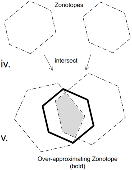
(b) Diffusion update step.

Figure 1: Strip-based approach in Algorithm 1, where (a) illustrates Lemma 1 and (b) illustrates Theorem 1.

2 Problem Statement and Preliminaries

We start by stating some preliminaries before describing our problem statement.

Definition 1.

(Zonotope [42]) A zonotope $\mathcal{Z}$ consists of a center $c\in{\mathbb{R}}^{n}$ and a generator matrix $G$ $\in$ ${\mathbb{R}}^{n\times e}$. We compose $G$ of $e$ generators $g^{(i)}\in{\mathbb{R}}^{n}$, $i=1,\dots,e$, where $G=\begin{bmatrix}g^{(1)},\dots,g^{(e)}\end{bmatrix}$.

$$\mathcal{Z}=\Big{\{}c+\sum\limits_{i=1}^{e}\beta^{(i)}g^{(i)}\Big{|}-1\leq\beta^{(i)}\leq 1\Big{\}}.$$ (1)

We use the shorthand $\mathcal{Z}=\langle c,G\rangle$ for a zonotope.

Given two zonotopes $\mathcal{Z}_{1}=\langle c_{1},G_{1}\rangle$ and $\mathcal{Z}_{2}=\langle c_{2},G_{2}\rangle$, the following operations can be computed exactly [42]:

1. Minkowski sum:

   $$\mathcal{Z}_{1}\oplus\mathcal{Z}_{2}=\Big{\langle}c_{1}+c_{2},[G_{1},G_{2}]\Big{\rangle}.$$ (2)

2. Linear map:

   $$L\mathcal{Z}_{1}=\Big{\langle}Lc_{1},LG_{1}\Big{\rangle}.$$ (3)

Let $C\in{\mathbb{R}}^{n\times p}$, then $\|C\|_{F}=\sqrt{\text{tr}(C^{T}C)}$ is the Frobenius norm of $C$. The Frobenius norm of a vector $x\in{\mathbb{R}}^{n}$ equals the Euclidean norm of the vector defined as $\|x\|=\sqrt{x^{T}x}$. The F-radius of the zonotope $\mathcal{Z}=\langle c,G\rangle$ is the Frobenius norm of the generator matrix. We denote the reduction operator by $\downarrow_{q}G$ of a generator matrix $G$. It basically reduces the number of generators of a zonotope to a fixed number $q$ so that the resulting zonotope is an over-approximation [43]. The operator diag($x$) returns a diagonal matrix with $x$ on the diagonal. Finally, for a scalar $c$ and matrices $A$, $B$ and $C$, we provide the following trace properties [44, p.11], where $\nabla_{X}f(X)$ is the derivative of $f(X)$ with respect to $X$:

$$\text{tr}(cA)=c\ \text{tr}(A),$$ (4)

$$\text{tr}(A+B)=\text{tr}(A)+\text{tr}(B),$$ (5)

$$\nabla_{X}\text{tr}(AXBX^{T}C)=A^{T}C^{T}XB^{T}+CAXB,$$ (6)

$$\nabla_{X}\text{tr}(B^{T}X^{T}CXB)=C^{T}XBB^{T}+CXBB^{T}.$$ (7)

We aim to estimate the set of possible states in a distributed fashion starting from the initial set $\mathcal{Z}_{0}$ by observing physical signals through sensory devices. Consider a set of $N$ nodes indexed by $i\in\{0,\ldots,N-1\}$ distributed geographically over some region. We denote the neighborhood of a given node $i$ by the set $\mathcal{N}_{i}$ containing $m_{i}$ nodes connected to node $i$, including the node itself. Every node is interested in estimating the set of possible states of the network state. The noise is assumed to be is unknown but bounded by a known bound and the initial set $\mathcal{Z}_{0}$ is known. We consider an observable discrete-time linear system model:

$$\begin{split}x_{k+1}&=Fx_{k}+n_{k},\\ y^{i}_{k}&=H^{i}x_{k}+v_{k}^{i},\end{split}$$ (8)

where $x_{k}\in\mathbb{R}^{n}$ is the state at time step $k$, $y^{i}_{k}\in\mathbb{R}^{p}$ the measurement observed by node $i$ at time step $k$, $F\in\mathbb{R}^{n\times n}$ the state matrix, $H^{i}\in\mathbb{R}^{p\times n}$ the measurement matrix, $n_{k}$ the process noise, and $v_{k}^{i}$ the measurement noise. The process and measurement noises are assumed to be unknown but bounded by zonotopes: $n_{k}\in\mathcal{Z}_{Q,k}=\langle 0,Q_{k}\rangle$ and $v_{k}^{i}\in\mathcal{Z}_{r,k}^{i}=\langle 0,\text{diag}(r^{i}_{k})\rangle$. If these zonotopes are not centered around zero, we perform a coordinate transformation. All vectors and matrices are real-valued and have proper dimensions.

3 Distributed Strip-based Diffusion Observer

As mentioned in the introduction, we focus on two types of set-based observers: strip-based observers and set-propagation observers. We propose two algorithms extending the related work of both observers and adding the set-based diffusion step to both observers. Our contribution to strip-based observers is presented first. We denote the state estimated at node $i$ of the strip-based approach by $\hat{x}_{s,k}^{i}$ for time step $k$. The set of possible states in strip-based approaches are generally obtained from predicted, measurement, and corrected state sets, which are defined as follows:

Definition 2.

(Predicted State Set) Given the system in (8) with initial zonotope $\hat{\mathcal{Z}}^{i}_{s,0}=\mathcal{Z}_{0}$, then the predicted reachable set $\hat{\mathcal{Z}}_{s,k}^{i}$ considering the zonotope $\mathcal{Z}_{Q,k}$ which bounds the modeling noise is defined as:

$$\hat{\mathcal{Z}}_{s,k}^{i}=F\hat{\mathcal{Z}}_{s,k-1}^{i}\oplus\mathcal{Z}_{Q,k}.$$ (9)

Definition 3.

(Measurement State Set) Given the system in (8), then the measurement state set $\mathcal{S}^{i}_{k}$ of node $i$ is defined as the set of all possible solutions $x_{k}$ given $y_{k}^{i}$ and $v_{k}^{i}\in\mathcal{Z}_{r,k}^{i}=\langle 0,\text{diag}(r^{i}_{k})\rangle$. If the dimension of $y_{k}^{i}\in\mathbb{R}^{p}$ equals one, i.e., $p=1$, this measurement set is a strip:

$$\mathcal{S}^{i}_{k}=\Big{\{}x_{k}\Big{|}|H^{i}x_{k}-y^{i}_{k}|\leq r^{i}_{k}\Big{\}},$$ (10)

and $\mathcal{S}^{i}_{k}$ is the intersection of multiple strips for $p>1$.

Definition 4.

(Corrected State Set) Given the system in (8) with initial set $\mathcal{Z}_{0}$, then the reachable corrected state set $\bar{\mathcal{Z}}_{s,k}^{i}$ of node $i$ is defined as the over-approximation of the intersection between $\hat{\mathcal{Z}}_{s,k}^{i}$ and $\mathcal{S}^{i}_{k}$:

$$\big{(}\hat{\mathcal{Z}}_{s,k}^{i}\cap\mathcal{S}^{i}_{k}\big{)}\subseteq\bar{\mathcal{Z}}_{s,k}^{i}.$$ (11)

Our proposed strip-based approach consists of three steps: measurement update, diffusion update, and time update. The time update step results in computing the predicted set (Definition 2). The measurement update step utilizes the previously predicted set along with the measurement set (Definition 3) to compute the corrected set (Definition 4). Every node in a distributed setting has access to some, not all, measurements. Therefore, we propose sharing measurements and estimated sets in the measurement and diffusion update steps, respectively, to obtain a lightweight consensus between the distributed nodes. We first give a high-level description of the proposed algorithm in Algorithm 1, then we derive the required theory. Our approach corrects the reachable set of each node by determining the set of consistent states with the model and measurements received from all neighbors. More specifically, during the measurement update, every node collects measurements from neighbors, as shown in step i in Figure 1(a), i.e., each node obtains a family of strips (measurements) to be intersected with the predicted zonotopic set (step ii in Figure 1(a)) of each node to obtain the estimated zonotope $\bar{\mathcal{Z}}^{i}_{s,k}$, dashed in step iii in Figure 1(a). Every node collects the shared sets from its neighbors in step iv in Figure 1(b). Next, each node intersects its reachable set with shared sets of the neighbors in the set-based diffusion step in step v in Figure 1(b). Finally, the estimated sets evolve according to the time update model.

Let $\Gamma^{i}=\begin{bmatrix}H^{1^{T}},\ldots,H^{m_{i}^{T}}\end{bmatrix}^{T}$, $\bar{y}^{i}_{k}=\begin{bmatrix}y^{{1}^{T}}_{k},\ldots,y^{m_{i}^{T}}_{k}\end{bmatrix}^{T}$, and $\bar{v}^{i}_{k}=\begin{bmatrix}v^{{1}^{T}}_{k},\ldots,v^{m_{i}^{T}}_{k}\end{bmatrix}^{T}\in\mathcal{Z}_{R,k}=\langle 0,R^{i}_{k}\rangle$, where $R^{i}_{k}=\text{diag}\Big{(}\begin{bmatrix}r^{{1}^{T}}_{k},\ldots,r^{m_{i}^{T}}_{k}\end{bmatrix}^{T}\Big{)}$ with $m_{i}$ equals the number of available measurements from the node’s neighbors. We propose to perform the measurement update step according to the following lemma [40], which is represented graphically in Figure 1(a):

Lemma 1 ([40]).

Given are the zonotope $\hat{\mathcal{Z}}_{s,k-1}^{i}=\big{\langle}\hat{c}^{i}_{s,k-1},$
$\hat{G}^{i}_{s,k-1}\big{\rangle}$, the family of $m_{i}$ measurement sets $\mathcal{S}^{i}_{k}$ in (10), and the design parameters $\Lambda^{i}_{s,k}$. The intersection between the zonotope and measurement sets can be over-approximated by a zonotope $\bar{\mathcal{Z}}^{i}_{s,k}=\big{\langle}\bar{c}^{i}_{s,k},\bar{G}^{i}_{s,k}\big{\rangle}$, where

$$\bar{c}^{i}_{s,k} =\hat{c}^{i}_{s,k-1}+\Lambda^{i}_{s,k}(\bar{y}^{i}_{k}-\Gamma^{i}\hat{c}^{i}_{s,k-1}),$$ (12)

$$\bar{G}^{i}_{s,k} =\Big{[}(I-\Lambda_{s,k}^{i}\Gamma^{i})\hat{G}^{i}_{s,k-1},\Lambda_{s,k}^{i}R^{i}_{k}\Big{]}.$$ (13)

The matrix of design parameters $\Lambda^{i}_{s,k}$ minimizing the Frobenius norm of the zonotope is obtained as in [45].

Algorithm 1 Distributed Strip-Based Diffusion Observer

Start with initial zonotope $\bar{\mathcal{Z}}_{s,k}^{i}=\mathcal{Z}_{0}$ for all nodes, and compute at every node $i$ and time instant $k$ the following:

Step 1: Measurement update:

$$\Lambda^{i}_{s,k} =\operatorname*{argmin}_{\Lambda^{i}_{s,k}}\|\bar{G}^{i}_{s,k}\|_{F}$$

$$\bar{c}^{i}_{s,k} =\hat{c}^{i}_{s,k-1}+\Lambda^{i}_{s,k}(\bar{y}^{i}_{k}-\Gamma^{i}\hat{c}^{i}_{s,k-1})$$

$$\bar{G}^{i}_{s,k} =\Big{[}(I-\Lambda_{s,k}^{i}\Gamma^{i})\hat{G}^{i}_{s,k-1},\Lambda_{s,k}^{i}R^{i}_{k}\Big{]}$$

Step 2: Diffusion update:

$$\mathfrak{w}^{i}_{k}= \operatorname*{argmin}_{\mathfrak{w}^{i}_{k}}\|\grave{G}_{s,k}^{i}\|_{F}.$$

$$\grave{c}^{i}_{s,k}= \frac{1}{\sum\limits_{j\in\mathcal{N}_{i}}w^{i,j}_{k}}\sum\limits_{j\in\mathcal{N}_{i}}w^{i,j}_{k}\bar{c}_{s,k}^{j}$$

$$\grave{G}_{s,k}^{i}= \frac{1}{\sum\limits_{j\in\mathcal{N}_{i}}w^{i,j}_{k}}\big{[}w^{i,1}_{k}\bar{G}^{1}_{s,k},...,w^{i,m_{i}}_{k}\bar{G}^{m_{i}}_{s,k}\big{]}$$

$$\tilde{G}_{s,k}^{i}= \downarrow_{q}{\grave{G}_{s,k}^{i}}$$

Step 3: Time update:

$$\hat{c}_{s,k}^{i}= F\grave{c}^{i}_{s,k}$$

$$\hat{G}_{s,k}^{i}= [F\tilde{G}_{s,k}^{i},Q_{k}]$$

As previously mentioned, every node shares its corrected zonotope $\bar{\mathcal{Z}}^{i}_{s,k}=\langle\bar{c}^{i}_{s,k},\bar{G}^{i}_{s,k}\rangle$ with its neighbours during the set-based diffusion step. We find the intersection between the shared zonotopes using the following theorem:

Theorem 1.

The intersection between $m_{i}$ zonotopes $\bar{\mathcal{Z}}^{j}_{s,k}=\langle\bar{c}^{j}_{s,k},\bar{G}^{j}_{s,k}\rangle$, $\forall j\in\mathcal{N}_{i}$, can be over-approximated by the zonotope $\grave{\mathcal{Z}}^{i}_{s,k}=\langle\grave{c}^{i}_{s,k},\grave{G}_{s,k}^{i}\rangle$ with

$$\grave{c}^{i}_{s,k} = \frac{1}{\sum\limits_{j\in\mathcal{N}_{i}}w^{i,j}_{k}}\sum\limits_{j\in\mathcal{N}_{i}}w^{i,j}_{k}\bar{c}_{s,k}^{j},$$ (14)

$$\grave{G}_{s,k}^{i} = \frac{1}{\sum\limits_{j\in\mathcal{N}_{i}}w^{i,j}_{k}}\big{[}w^{i,1}_{k}\bar{G}^{1}_{s,k},...,w^{i,m_{i}}_{k}\bar{G}^{m_{i}}_{s,k}\big{]},$$ (15)

where $w^{i,j}_{k}$ is a weight such that $\sum\limits_{j\in\mathcal{N}_{i}}w^{i,j}_{k}\neq 0$.

Proof.

We aim to find the zonotope which over-approximates the intersection. Let $\bar{x}\in(\bar{\mathcal{Z}}^{1}_{s,k}\cap\bar{\mathcal{Z}}^{2}_{s,k}\cap...\cap\bar{\mathcal{Z}}^{m_{i}}_{s,k})$ then $\bar{x}$ is within the zonotope defined in (1), i.e., we have $z^{j}\in[-1,1]$ for each zonotope $j$ such that

$$\bar{x}=\bar{c}^{j}_{s,k}+\bar{G}^{j}_{s,k}z^{j}.$$ (16)

By multiplying (16) with $w^{i,j}_{k}$ and summing for all $m_{i}$ zonotopes, we obtain

$$\bar{x} =\underbrace{\frac{1}{\sum\limits_{j\in\mathcal{N}_{i}}w^{i,j}_{k}}\sum\limits_{j\in\mathcal{N}_{i}}w^{i,j}_{k}\bar{c}_{s,k}^{j}}_{\grave{c}^{i}_{s,k}}$$

$$+\underbrace{\frac{1}{\sum\limits_{j\in\mathcal{N}_{i}}w^{i,j}_{k}}\big{[}w_{k}^{i,1}\bar{G}^{1}_{s,k},...,w_{k}^{i,{m_{i}}}\bar{G}^{m_{i}}_{s,k}\big{]}}_{\grave{G}^{i}_{s,k}}\underbrace{\begin{bmatrix}z^{1}\\ \vdots\\ z^{m_{i}}\end{bmatrix}}_{\textbf{z}}$$

$$=\grave{c}^{i}_{s,k}+\grave{G}^{i}_{s,k}\textbf{z}.$$ (17)

Note that $\textbf{z}\in[-\textbf{1},\textbf{1}]$ as $z^{1},\dots,z^{m_{i}}\in[-1,1]$. Thus, the center and the generator of the over-approximating zonotope are $\grave{c}^{i}_{s,k}$ and $\grave{G}^{i}_{s,k}$, respectively. ∎

The optimal design of the weight vector $\mathfrak{w}^{i}_{k}=\Big{[}w^{i,1}_{k},\dots,$ $w^{i,m_{i}}_{k}\Big{]}$ can be chosen such that the size of the zonotope $\grave{\mathcal{Z}}^{i}_{s,k}=\langle\grave{c}^{i}_{s,k},\grave{G}_{s,k}^{i}\rangle$ is minimal. Using the Frobenius norm as an indicator of zonotopic size, we compute $\mathfrak{w}^{i}_{k}$ by solving

$$\mathfrak{w}^{i}_{k}=\operatorname*{argmin}_{\mathfrak{w}^{i}_{k}}\|\grave{G}_{s,k}^{i}\|_{F}.$$ (18)

Next, we add the constraint $\sum\limits_{j\in\mathcal{N}_{i}}w^{i,j}_{k}=1$ in order to facilitate finding the optimal weights $w^{i,j}_{k}$ in the following proposition.

Proposition 1.

For the over-approximated set $\grave{\mathcal{Z}}^{i}_{s,k}$ $=\langle\grave{c}^{i}_{s,k}$, $\grave{G}_{s,k}^{i}\rangle$ in Theorem 1, the optimal design parameters $w^{i,j}_{k}$ for (18), $\forall j\in\mathcal{N}_{i}$ where $\sum\limits_{j\in\mathcal{N}_{i}}w^{i,j}_{k}=1$, can be obtained as:

$$w^{i,j}_{k}=\frac{1}{\text{tr}\Big{(}\bar{G}^{j}_{s,k}\bar{G}_{s,k}^{j^{T}}\Big{)}\sum\limits_{r\in\mathcal{N}_{i}}\frac{1}{\text{tr}\Big{(}\bar{G}^{r}_{s,k}\bar{G}_{s,k}^{r^{T}}\Big{)}}}.$$ (19)

Proof.

The Frobenius norm of the generator matrix can be computed as follows:

$$\|\grave{G}_{s,k}^{i}\|^{2}_{F} = \text{tr}\Big{(}\grave{G}_{s,k}^{i}\grave{G}_{s,k}^{i^{T}}\Big{)}$$ (20)

$$\stackrel{{\scriptstyle\eqref{eq:gdiff}}}{{=}} \text{tr}\Big{(}\sum\limits_{r\in\mathcal{N}_{i}}(w^{i,r}_{k})^{2}\bar{G}^{r}_{s,k}\bar{G}^{r^{T}}_{s,k}\Big{)}$$

$$\stackrel{{\scriptstyle\eqref{eq:trMatpMat}}}{{=}} \sum\limits_{r\in\mathcal{N}_{i}}\text{tr}\Big{(}(w^{i,r}_{k})^{2}\bar{G}^{r}_{s,k}\bar{G}^{r^{T}}_{s,k}\Big{)}$$

$$\stackrel{{\scriptstyle\eqref{eq:trscalMat}}}{{=}} \sum\limits_{r\in\mathcal{N}_{i}}(w^{i,r}_{k})^{2}\text{tr}\Big{(}\bar{G}^{r}_{s,k}\bar{G}^{r^{T}}_{s,k}\Big{)}.$$

Let $\alpha_{r}=\text{tr}\Big{(}\bar{G}^{r}_{s,k}\bar{G}^{r^{T}}_{s,k}\Big{)}$, therefore we obtain the following constrained optimization problem:

$$w^{i,j}_{k}=\operatorname*{argmin}_{w^{i,j}_{k}}\sum\limits_{r\in\mathcal{N}_{i}}\alpha_{r}(w^{i,r}_{k})^{2},$$

$$\text{subject to}{\ }f(\mathfrak{w}^{i}_{k})=\sum\limits_{r\in\mathcal{N}_{i}}w^{i,r}_{k}-1=0.$$ (21)

This can be solved by introducing the Lagrange multiplier $s$ [46]. The Lagrangian function for (21) is

$$\mathcal{L}=\sum\limits_{r\in\mathcal{N}_{i}}\alpha_{r}(w^{i,r}_{k})^{2}-s\Bigg{(}\sum\limits_{r\in\mathcal{N}_{i}}w^{i,r}_{k}-1\Bigg{)}.$$ (22)

The necessary condition $\forall j\in\mathcal{N}_{i}$ for an extremum point is

$$\nabla_{w^{i,j}_{k}}\mathcal{L}=2w^{i,j}_{k}\alpha_{j}-s=0.$$ (23)

Inserting (23) in (21) results in:

$$s=\frac{2}{\sum\limits_{r\in\mathcal{N}_{i}}\frac{1}{\alpha_{r}}}.$$ (24)

Inserting (24) into (23) results in:

$$w^{i,j}_{k}\stackrel{{\scriptstyle\eqref{eq:derv_w}}}{{=}}\frac{s}{2\alpha_{j}}\stackrel{{\scriptstyle\eqref{eq:s}}}{{=}}\frac{1}{\alpha_{j}\sum\limits_{r\in\mathcal{N}_{i}}\frac{1}{\alpha_{r}}}.$$ (25)

It remains to check if the extremum point is a minimum [47]. We compute the bordered Hessian matrix $H^{b}$, while suppressing the indices $i$ and $k$, and denoting $\nabla_{w^{j}}X(\mathfrak{w})$ by $X_{w^{j}}$ and $\nabla_{w^{j}w^{m}}X(\mathfrak{w})$ by $X_{w^{j,{m}}}$ for simplicity:

$$H^{b} =\begin{bmatrix}0&-f_{w^{1}}&\dots&-f_{w^{m}}\\ -f_{w^{1}}&\mathcal{L}_{w^{1,1}}&\dots&\mathcal{L}_{w^{1,{m}}}\\ \vdots&\vdots&\ddots&\vdots\\ -f_{w^{m}}&\mathcal{L}_{w^{{m},1}}&\dots&\mathcal{L}_{w^{{m},{m}}}\end{bmatrix}$$

$$=\begin{bmatrix}0&-1&-1&\dots&-1\\ -1&2\alpha_{1}&0&\dots&0\\ -1&0&2\alpha_{2}&\dots&0\\ \vdots&\vdots&&\ddots&\\ -1&0&0&\dots&2\alpha_{m}\end{bmatrix}.$$ (26)

The $m-1$ largest principal minors of (26) are negatives because $\alpha_{r}$ is positive $\forall\,r=1,\dots,m$. Thus, the extremum in (25) is a minimum point, which concludes the proof. ∎

After presenting our distributed strip-based approach using the diffusion strategy, we present our set-propagation diffusion observer.

4 Distributed Set-Propagation Diffusion Observer

Unlike the strip-based observer developed in the previous section, which was based on geometric intersection, we propose the following set-propagation observer based on the following structure while bounding the unknown noise by the corresponding bounding zonotope:

$$x_{k}^{i}=Fx_{k-1}^{i}+n_{k}+\Lambda^{i}_{v,k}(\bar{y}^{i}_{k}-\Gamma^{i}x^{i}_{k-1}-\bar{v}^{i}_{k})$$ (27)

where $\Lambda^{i}_{v,k}$ is a time-varying observer gain computed at each time step. The design of the observer makes use of the bounds of the noises. Let $x_{v,k}^{i}$ be the state estimated by the set-propagation observer. For the distributed system in (8), the proposed design consists of two steps: Luenberger update and diffusion update. During the Luenberger update, every node shares its measurement with its neighbour, while in the diffusion step, every node shares the estimated information with its neighbours. We first discuss the Luenberger update step.

Theorem 2.

Given are the system in (8), the measurements $y^{i}_{k}$, several zonotopes bounding $\hat{x}^{i}_{v,0}\in\mathcal{Z}_{0}$, $n_{k}\in\mathcal{Z}_{Q,k}=\langle 0,Q_{k}\rangle$, $\bar{v}_{k}^{i}\in\mathcal{Z}^{i}_{R,k}=\langle 0,R_{k}^{i}\rangle$, and the state $\hat{x}^{i}_{v,k-1}\in\Big{\langle}\hat{c}^{i}_{v,k-1}$, $\hat{G}^{i}_{v,k-1}\Big{\rangle}$. The zonotope bounding the uncertain states can be iteratively obtained as $\hat{x}^{i}_{v,k}\in\Big{\langle}\bar{c}^{i}_{v,k},\bar{G}^{i}_{v,k}\Big{\rangle}$, where

$$\bar{c}^{i}_{v,k}= F\hat{c}^{i}_{v,k-1}+\Lambda_{v,k}^{i}\Big{(}\bar{y}^{i}_{k}-\Gamma^{i}\hat{c}^{i}_{v,k-1}\Big{)},$$ (28)

$$\bar{G}^{i}_{v,k}= \Big{[}\Big{(}F-\Lambda_{v,k}^{i}\Gamma^{i}\Big{)}\hat{G}^{i}_{v,k-1},-\Lambda_{v,k}^{i}R_{k}^{i},Q_{k}\Big{]}.$$ (29)

Proof.

Given $\hat{x}_{v,k-1}^{i}\in\Big{\langle}\hat{c}_{v,k-1}^{i},\hat{G}_{v,k-1}^{i}\Big{\rangle}$, $n_{k}\in\mathcal{Z}_{Q,k}$ $=\langle 0$ $,Q_{k}\rangle$, and $\bar{v}_{k}^{i}\in\mathcal{Z}_{R,k}^{i}=\langle 0,R_{k}^{i}\rangle$, and by using (27), one obtains:

$$\hat{x}_{v,k}^{i}\in\Big{\langle}\bar{c}_{v,k}^{i},\bar{G}_{v,k}^{i}\Big{\rangle}$$

$$\stackrel{{\scriptstyle\eqref{Eq:LO}}}{{=}}\Big{(}F-\Lambda_{v,k}^{i}\Gamma^{i}\Big{)}\hat{\mathcal{Z}}_{v,k-1}^{i}\oplus\mathcal{Z}_{Q,k}$$

$$\quad\oplus\Big{\langle}\Lambda_{v,k}^{i}\bar{y}^{i}_{k},0\Big{\rangle}\oplus-\Lambda^{i}_{v,k}\mathcal{Z}_{R,k}$$

$$=\Big{(}F-\Lambda_{v,k}^{i}\Gamma^{i}\Big{)}\Big{\langle}\hat{c}^{i}_{v,k-1},\hat{G}^{i}_{v,k-1}\Big{\rangle}\oplus\langle 0,Q_{k}\rangle$$

$$\quad\oplus\Big{\langle}\Lambda_{v,k}^{i}\bar{y}^{i}_{k},0\Big{\rangle}\!\oplus\!\Big{\langle}0,-\Lambda_{v,k}^{i}R_{k}^{i}\Big{\rangle}$$

$$\stackrel{{\scriptstyle\eqref{eq:minkowski},\eqref{eq:linmap}}}{{=}}\Bigg{\langle}\underbrace{\Big{[}F\hat{c}^{i}_{v,k-1}+\Lambda_{v,k}^{i}\Big{(}\bar{y}^{i}_{k}-\Gamma^{i}\hat{c}^{i}_{v,k-1}\Big{)}\Big{]}}_{\bar{c}_{v,k}^{i}},$$

$$\quad\underbrace{\Big{[}\Big{(}F-\Lambda_{v,k}^{i}\Gamma^{i}\Big{)}\hat{G}^{i}_{v,k-1},-\Lambda_{v,k}^{i}R_{k}^{i},Q_{k}\Big{]}}_{\bar{G}_{v,k}^{i}}\Bigg{\rangle}$$

∎

Algorithm 2 Distributed Set-Propagation Diffusion Observer

Start with initial zonotope $\bar{\mathcal{Z}}_{v,k}^{i}=\mathcal{Z}_{0}$ for all nodes, and at every time instant $k$, compute at every node $i$:

Step 1: Luenberger update:

$$\Lambda^{i}_{v,k} = \operatorname*{argmin}_{\Lambda^{i}_{v,k}}\|\bar{G}^{i}_{v,k}\|_{F}$$

$$\bar{c}^{i}_{v,k} = F\hat{c}^{i}_{v,k-1}+\Lambda_{v,k}^{i}\Big{(}\bar{y}^{i}_{k}-\Gamma^{i}\hat{c}^{i}_{v,k-1}\Big{)}$$

$$\bar{G}^{i}_{v,k} = \Big{[}\Big{(}F-\Lambda_{v,k}^{i}\Gamma^{i}\Big{)}\hat{G}^{i}_{v,k-1},-\Lambda_{v,k}^{i}R_{k}^{i},Q_{k}\Big{]}$$

Step 2: Diffusion update:

$$\mathfrak{w}_{k}^{i} = \operatorname*{argmin}_{\mathfrak{w}_{k}^{i}}\|\tilde{G}_{v,k}^{i}\|_{F}.$$

$$\hat{c}^{i}_{v,k} = \frac{1}{\sum\limits_{j\in\mathcal{N}_{i}}w^{i,j}_{k}}\sum\limits_{j\in\mathcal{N}_{i}}w^{i,j}_{k}\bar{c}_{v,k}^{j}$$

$$\tilde{G}_{v,k}^{i} = \frac{1}{\sum\limits_{j\in\mathcal{N}_{i}}w^{i,j}_{k}}\big{[}w^{i,1}_{k}\bar{G}^{1}_{v,k},\dots,w^{i,m_{i}}_{k}\bar{G}^{m_{i}}_{v,k}\big{]}$$

$$\hat{G}_{v,k}^{i} = \downarrow_{q}{\tilde{G}_{v,k}^{i}}$$

We propose to compute the design vectors $\Lambda^{i}_{v,k}$ according to [9] such that:

$$\Lambda^{i}_{v,k}=\operatorname*{argmin}_{\Lambda^{i}_{v,k}}\|\bar{G}^{i}_{v,k}\|_{F},$$ (30)

which is a lightweight indication of the volume to decrease the computation cost and maintain a good performance. The following proposition is provided to compute the optimal parameters $\Lambda^{i}_{v,k}$.

Proposition 2.

For the estimated zonotopic set $\hat{\mathcal{Z}}^{i}_{v,k}=\langle\hat{c}^{i}_{v,k-1}$, $\hat{G}^{i}_{v,k-1}\rangle$ corresponding to node $i$, the optimal design parameters $\Lambda^{i}_{v,k}$ for (30) can be obtained as:

$$\Lambda^{i}_{v,k}=\frac{F\hat{G}^{i}_{v,k-1}\hat{G}^{i^{T}}_{v,k-1}\Gamma^{i^{T}}}{\Gamma^{i}\hat{G}^{i}_{v,k-1}\hat{G}^{i^{T}}_{v,k-1}\Gamma^{i^{T}}+R_{k}^{i}R_{k}^{i^{T}}}.$$ (31)

Proof.

The proof is along the lines of [45]. The Frobenious norm of (29) can be computed as

$$\|\bar{G}^{i}_{v,k}\|^{2}_{F}= \text{tr}\ (\bar{G}^{i}_{v,k}\bar{G}^{i^{T}}_{v,k})$$

$$\stackrel{{\scriptstyle\eqref{eq:Gf_lambda2}}}{{=}} \text{tr}\ \Bigg{(}\Big{(}F-\Lambda^{i}_{v,k}\Gamma^{i}\Big{)}\mathcal{G}\Big{(}F-\Lambda^{i}_{v,k}\Gamma^{i}\Big{)}^{T}$$

$$+\Lambda^{i}_{v,k}\mathcal{R}^{i}\Lambda^{i^{T}}_{v,k}+Q_{k}Q_{k}^{T}\Bigg{)}$$

$$= \text{tr}\Big{(}F\mathcal{G}F^{T}-F\mathcal{G}\Gamma^{i^{T}}\Lambda^{i^{T}}_{v,k}-\Lambda^{i}_{v,k}\Gamma^{i}\mathcal{G}F^{T}$$

$$+\Lambda^{i}_{v,k}\Gamma^{i}\mathcal{G}\Gamma^{i^{T}}\Lambda^{i^{T}}_{v,k}+\Lambda^{i}_{v,k}\mathcal{R}^{i}\Lambda^{i^{T}}_{v,k}{+}Q_{k}Q_{k}^{T}\Big{)},$$ (32)

where $\mathcal{R}^{i}=R_{k}^{i}R_{k}^{i^{T}}$ and $\mathcal{G}=\hat{G}^{i}_{s,{k-1}}\hat{G}^{i^{T}}_{s,{k-1}}$. The optimal value of $\Lambda^{i}_{v,k}$ can be obtained by solving

$$\nabla_{\scaleto{\Lambda}{3.5pt}^{i}_{v,k}}\|\bar{G}^{i}_{v,k}\|^{2}_{F}=0,$$ (33)

where the Jacobian in (33) can be computed by applying matrix properties in (6) and (7) to (32):

$$\nabla_{\scaleto{\Lambda}{3.5pt}^{i}_{v,k}}\|\bar{G}^{i}_{v,k}\|^{2}_{F} = -2F\mathcal{G}\Gamma^{i^{T}}+2\Lambda^{i}_{v,k}\Gamma^{i}\mathcal{G}\Gamma^{i^{T}}+2\Lambda^{i}_{v,k}\mathcal{R}^{i}$$ (34)

$$= 0$$

By inserting the optimal $\Lambda^{i}_{v,k}$ from (31) in (34), one can see that (34) is fulfilled. We do not have to check the type of extremum since we have an unconstrained norm, which is always convex. ∎

Following the Luenberger update step, in the diffusion step, each node shares the information of the estimated zonotope $\langle\bar{c}^{i}_{v,k},\bar{G}^{i}_{v,k}\rangle$ with its neighbours. The intersection between the shared zonotopes is then computed as discussed earlier in Theorem 1. The iterative design of the above two-step Luenberger observer is provided in Algorithm 2. We note that one of the differences between the introduced set-propagation observer and strip-based observer is the position of the time update step. This appears by comparing Theorem 2 with Theorem 1. Also, it can be easily shown that

$$\Lambda^{i}_{v,k}=F\Lambda^{i}_{s,k}.$$ (35)

5 Comparison to Diffusion Kalman Filter

In this section, we build the analogy with the diffusion Kalman filter (DKF) [48]. We start by defining the Gaussian random vectors $n_{k}\sim\mathcal{N}(0,\bar{Q}_{k})$ and $v_{k}^{i}\sim\mathcal{N}(0,\bar{R}_{k}^{i})$ where $\mathcal{N}(\mu,\Sigma)$ denotes a Gaussian distribution with mean $\mu$ and covariance $\Sigma$. We start by showing the analogy with the incremental update, then we show it for the diffusion update.

5.1 Incremental Update

Corresponding to incremental update in DKF we have for every node $i$ with a neighbor node $j$ [48]

$${S}^{i}_{k}=\bar{R}^{i}_{k}+H^{i}{P}^{i}_{k-1}H^{i^{T}},$$

$$\bar{x}^{i}_{k}=\hat{x}^{i}_{k-1}+{P}^{i}_{k-1}H^{i^{T}}{S}_{k}^{i^{-1}}(y^{j}_{k}-H^{i}\hat{x}_{k-1}^{i}),$$

$${P}^{i}_{k}={P}^{i}_{k-1}-{P}^{i}_{k-1}H^{i^{T}}{S}_{k-1}^{i^{-1}}H^{i}{P}^{i}_{k-1}.$$

Let us introduce

$$L_{k}={P}^{i}_{k-1}H^{i^{T}}{S}_{k}^{i^{-1}}.$$ (36)

Then after the incremental update, the center estimate corresponding to each node can be expressed using the gain $L_{k}$ as

$$\bar{x}^{i}_{k} =\hat{x}^{i}_{k-1}+L_{k}(y^{j}_{k}-H^{i}\hat{x}_{k-1}^{i}).$$ (37)

We have from (31) and (35)

$$\Lambda^{i}_{s,k}=\frac{\hat{G}^{i}_{s,k-1}\hat{G}^{i^{T}}_{s,k-1}\Gamma^{i^{T}}_{k}}{\Gamma^{i}_{k}\hat{G}^{i}_{s,k-1}\hat{G}^{i^{T}}_{s,k-1}\Gamma^{i^{T}}_{k}+R_{k}^{i}R_{k}^{i^{T}}},$$ (38)

Comparing (36) with (38) and (37) with (12) for a node $i$ with a single neighbor $j$ results in the following analogy

$$P^{i}_{k}\equiv\bar{G}^{i}_{s,k}\bar{G}_{s,k}^{i^{T}},\quad\bar{R}_{k}\equiv R_{k}^{i}R_{k}^{i^{T}},\quad\bar{x}^{i}_{k}\equiv\bar{c}^{i}_{s,k}.$$ (39)

5.2 Diffusion Update

The diffusion update in DKF can be expressed as

$$\hat{x}^{i}_{k} = \sum\limits_{j\in\mathcal{N}_{i}}w_{k}^{i,j}\bar{x}_{k}^{j},$$

which resembles our zonotopes intersection formula in (14) in case of $\sum\limits_{j\in\mathcal{N}_{i}}w_{k}^{i,j}=1$. Moreover, the optimal weight based on covariance intersection [49, Section III] is a function of $\frac{1}{tr(P^{j}_{k})\sum\limits_{r\in\mathcal{N}_{i}}\frac{1}{tr(P^{r}_{k})}}$ which again resembles our optimal weights in (19).

5.3 Discussion

Based on the above results, it can be said that if the initial center $c_{0}$ is chosen equally for the DKF and our strip-based observer along with the same initial covariance matrices $P_{0}=\hat{G}_{0}^{i}(\hat{G}_{0}^{i})^{T}$ and same diffusion weights, then in the absence of any over-approximation error due to the zonotopic reduction operation, both observers would result in the same optimal gain $L_{k}$ and return the same center estimate $\hat{x}^{i}_{k}$.

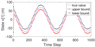
(a)

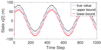
(b)

Figure 2: True values, upper bounds, and lower bounds of the two-dimensional estimated states using our strip-based approach in Algorithm 1. Every node has four neighbors.

6 Evaluation

Our proposed algorithms are implemented in Matlab 2019 on an example similar to the one presented in [39, 50], where a network of eight nodes attempts to track the position of a rotating object. We made use of CORA [51] for zonotope operations along with implementations from [52]. The state of each node consists of the unknown two-dimensional position of the rotating object. The state matrix in (8) is

$$F=\begin{bmatrix}0.992&-0.1247\\ 0.1247&0.992\end{bmatrix},$$ (40)

and the measurement matrix $H^{i}$ alternates between $[01]$ and $[10]$ in the sequence of the taken measurements. We run our proposed algorithms in comparison with the one proposed by Garcia et al. [53] and DKF [48] on the same generated data set. The related work in set-based methods does not consider sharing the measurements between the neighbors like our approach, and this affects the estimation results but comes at the cost of extra communication. Thus, we will analyze our algorithms with and without sharing the measurements for a fair comparison. Figure 2 shows the true values, upper bound, and lower bound for each dimension of the estimated state using the strip-based approach in Algorithm 1 while each node is connected to four neighbors. We start with a set ($160\times 160m^{2}$) covering the whole localization area at the initial point (time step $0$), then it becomes smaller due to receiving measurements and performing geometric intersection to correct the estimated state. In addition, we repeat the same experiments using Algorithm 2 and present the results in Figure 3.

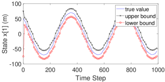
(a)

(b)

Figure 3: True values, upper bounds, and lower bounds of the two-dimensional estimated states using our set-propagation approach in Algorithm 2. Every node has four neighbors.

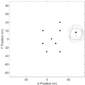
(a)

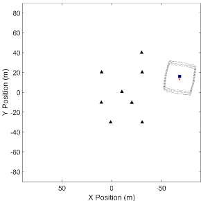
(b)

Figure 4: Snapshots of the estimated zonotopes with the red pluses as centers. The triangles are the true positions for the observing nodes. The blue rectangle is the true position of the rotating target. Figure 4(a) shows the distributed estimated zonotopes using Algorithm 2 without the diffusion step. Figure 4(b) shows Algorithm 2 with the diffusion step.

Table 1: The mean and standard deviation of the Hausdorff distance (m) between the estimated zonotopes in comparison to [53] and [48], where every node has two, four, or six neighbors. The results are presented with and without the diffusion step and sharing the measurements over different network connectivities.

			Six neighbors		Four neighbors		Two neighbors
Algorithm	Meas. sharing	Diffusion	mean	std	mean	std	mean	std
Alg. 1	✓	✓	0.242	0.160	0.824	0.409	2.813	2.163
Alg. 1	✗	✓	3.019	2.244	3.899	4.062	5.914	3.683
Alg. 1	✓	✗	1.517	1.393	2.703	2.118	3.829	2.360
Alg. 2	✓	✓	0.333	0.242	1.897	1.332	3.871	2.362
Alg. 2	✗	✓	1.601	1.846	3.202	2.889	5.760	3.607
Alg. 2	✓	✗	1.813	1.553	3.405	2.460	4.855	2.464
Garcia [53]	-	-	32.482	19.578	29.523	17.387	25.443	14.517
DKF [48]	-	-	0.195	0.129	0.680	0.420	2.811	2.099

The effect of the diffusion step is analyzed graphically over a network with low connectivity, where every node is connected to two nodes only. Snapshots of the estimated zonotopes by the distributed nodes in Algorithm 2 are shown in Figure 4. The triangles are the true positions of the monitoring nodes. The estimates are the centers of the zonotopes, which are represented by red pluses. Figure 4(a) and 4(b) show the results without and with the diffusion step, respectively. As shown in the aforementioned figures, the diffusion step allows the estimated zonotopes by the distributed nodes to partially consense on a set, which is one of the advantages of adding the diffusion step.

The Hausdorff distance measures how far two subsets of a metric space are from each other. Thus, as another measure of the estimated zonotope consistency for all the distributed nodes, we calculate the Hausdorff distance between each zonotope at different time steps. We analyze the Hausdorff distance over different network connectivities. The results are reported in Table 1 for DKF, Garcia et al. [53], Algorithms 1 and 2 with and without the diffusion step and measurements sharing between the neighbours. The diffusion step enhances the alignment between the estimated zonotopes, significantly affecting a network with low connectivity. For the aforementioned network, every node has access to a lower number of measurements, and thus the diffusion step provides more information to the distributed nodes and enhances the alignment of the estimated zonotopes, estimation results, and radii of the estimated zonotopes. The Hausdorff distance decreases with increasing the number of neighbors in Table 1 as the amount of shared information increases with increasing the connectivity. The set in the case of DKF is computed using the $3\sigma$ confidence interval of each node. The Hausdorff distance is smaller in the case of DKF; however, it comes without state containment guarantees.

Table 2: The mean and standard of the radius (m) of the estimated zonotopes by the proposed algorithms in comparison to [53] and [48]. The results are presented with and without the diffusion step and sharing the measurements over different network connectivities.

			Six neighbors		Four neighbors		Two neighbors
Algorithm	Meas. sharing	Diffusion	mean	std	mean	std	mean	std
Alg. 1	✓	✓	11.877	0.057	12.626	0.221	15.104	0.442
Alg. 1	✗	✓	22.267	3.507	24.405	2.969	26.973	4.012
Alg. 1	✓	✗	13.312	0.419	13.084	0.272	12.920	0.210
Alg. 2	✓	✓	13.266	1.235	13.515	0.432	15.257	0.393
Alg. 2	✗	✓	20.943	3.598	21.699	3.142	21.241	3.808
Alg. 2	✓	✗	16.690	1.443	17.174	0.918	18.531	1.330
Garcia [53]	-	-	53.681	21.992	49.932	19.373	44.671	16.040
DKF [48]	-	-	3.671	0.201	3.949	0.283	4.463	0.482

Table 3: The mean and standard deviation of the localization error (m) of the center of the estimated zonotopes using the proposed algorithms in comparison to [53] and [48] over different network connectivities, where every node has two, four, or six neighbors. The results are presented with and without the diffusion step and sharing the measurements over different network connectivities.

			Six neighbors		Four neighbors		Two neighbors
Algorithm	Meas. sharing	Diffusion	mean	std	mean	std	mean	std
Alg. 1	✓	✓	2.227	0.490	2.419	0.485	3.485	0.486
Alg. 1	✗	✓	3.145	4.226	3.020	4.095	3.980	4.471
Alg. 1	✓	✗	2.463	0.409	3.528	0.315	5.605	0.477
Alg. 2	✓	✓	1.495	0.513	0.892	0.415	4.882	0.871
Alg. 2	✗	✓	3.630	4.191	6.475	3.512	13.311	4.060
Alg. 2	✓	✗	2.489	0.489	3.550	0.459	5.853	0.761
Garcia [53]	-	-	11.729	1.573	11.877	1.571	12.059	1.717
DKF [48]	-	-	2.207	0.468	2.403	0.464	3.773	0.528

One important aspect of the performance of the set-based estimation algorithm is reducing the resulting radius of the over-approximating estimated set. Therefore, we analyze the radii of the estimated zonotopes of the proposed algorithms in comparison to the previous work in [53] and [48]. Table 2 shows the mean and standard deviation of the radii with and without the diffusion step and measurement sharing. The diffusion step and the measurement sharing decrease the radii due to the proposed intersection criteria. Moreover, our proposed algorithms with and without the diffusion step are much better than the previous work in [53]. We note that the network with higher connectivity has a smaller radius as the intersection with more strips decreases the estimated set. The center of the estimated zonotope is considered a single-point estimate of the proposed algorithms. Therefore, we report the localization error of the estimated centers by the proposed algorithms in Table 3. The diffusion significantly enhances the center estimate of the proposed algorithms. Again, the diffusion step is more effective in a network with a low connectivity.

Table 4 shows the execution time of each step in the proposed algorithms while again changing the number of neighbors. To measure the execution time, we run each step $500$ times with randomly generated zonotopes with $20$ generators and take the average execution time. The measurements were taken on an 11^th Generation Intel(R) Core(TM) i7-1185G7 processor with 16.0 GB RAM. The time update step does not depend on the number of neighbors.

Table 4: Execution time in $\mu$ seconds of the proposed measurement, diffusion, Luenberger, and time updates in Algorithms 1 and 2 with a different number of neighbors.

	Number of neighbors
Step	Six	Four	Two
Measurement update	$76$	$70$	$63$
Diffusion update	$64$	$48$	$31$
Time update	$24$	$24$	$24$
Luenberger update	$77$	$73$	$64$

The main challenges in proposing new set-based observers are mainly choosing the set representation. We chose zonotopes as one can efficiently compute linear maps and Minkowski sums – both are essential operations for set-based observers. In addition, selecting the appropriate optimization function for computing the observer gain, which can maintain low computation costs and high accuracy in comparison to the standard volume minimization technique, was a challenge. We ended up choosing the Frobenius norm as a lightweight indication of the volume of the zonotope.

7 Conclusion

We propose two distributed strip-based and set-propagation observers using a diffusion strategy. Our algorithms remove the need for a fusion center. They only require every node to communicate with its neighbors: first, to share the measurements and second, to share the estimates. The diffusion step ensures that information is propagated throughout the network in order to converge to the best estimate and provide consistency between the estimated sets. We propose a new over-approximation for zonotopes intersection to compose the diffusion step and evaluate our algorithms in a localization example of a rotating object.

References

- Grewal et al. [2020] M. S. Grewal, A. P. Andrews, C. G. Bartone, Kalman filtering, in: Global Navigation Satellite Systems, Inertial Navigation, and Integration, 2020, pp. 355–417.
- Puig [2010] V. Puig, Fault diagnosis and fault tolerant control using set-membership approaches: Application to real case studies, International Journal of Applied Mathematics and Computer Science 20 (2010) 619–635.
- Combastel [2015] C. Combastel, Merging Kalman filtering and zonotopic state bounding for robust fault detection under noisy environment, IFAC-PapersOnLine 48 (2015) 289–295.
- Wang et al. [2017] Y. Wang, Z. Wang, V. Puig, G. Cembrano, Zonotopic fault estimation filter design for discrete-time descriptor systems, IFAC-PapersOnLine 50 (2017) 5055–5060.
- Zhang et al. [2019] W. Zhang, Z. Wang, Y. Shen, S. Guo, F. Zhu, Interval estimation of actuator fault by interval analysis, IET Control Theory & Applications 13 (2019) 2717–2724.
- Combastel and Zolghadri [2018] C. Combastel, A. Zolghadri, FDI in cyber physical systems: A distributed zonotopic and Gaussian Kalman filter with bit-level reduction, IFAC-PapersOnLine 51 (2018) 776–783.
- Althoff and Rath [2021] M. Althoff, J. J. Rath, Comparison of guaranteed state estimators for linear time-invariant systems, Automatica 130 (2021) 109662.
- Pourasghar et al. [2016] M. Pourasghar, V. Puig, C. Ocampo-Martinez, Comparison of set-membership and interval observer approaches for state estimation of uncertain systems, in: European Control Conference, IEEE, 2016, pp. 1111–1116.
- Combastel [2015a] C. Combastel, Zonotopes and kalman observers: Gain optimality under distinct uncertainty paradigms and robust convergence, Automatica 55 (2015a) 265–273.
- Combastel [2015b] C. Combastel, Merging kalman filtering and zonotopic state bounding for robust fault detection under noisy environment, IFAC-PapersOnLine 48 (2015b) 289–295. 9th IFAC Symposium on Fault Detection, Supervision and Safety for Technical Processes Safe Process.
- Wang and Puig [2016] Y. Wang, V. Puig, Zonotopic extended kalman filter and fault detection of discrete-time nonlinear systems applied to a quadrotor helicopter, in: Conference on Control and Fault-Tolerant Systems, IEEE, 2016, pp. 367–372.
- Schweppe [1968] F. Schweppe, Recursive state estimation: Unknown but bounded errors and system inputs, IEEE Transactions on Automatic Control 13 (1968) 22–28.
- Gollamudi et al. [1998] S. Gollamudi, S. Nagaraj, S. Kapoor, Y.-F. Huang, Set-membership filtering and a set-membership normalized LMS algorithm with an adaptive step size, IEEE Signal Processing Letters 5 (1998) 111–114.
- Alamo et al. [2008] T. Alamo, J. M. Bravo, M. J. Redondo, E. F. Camacho, A set-membership state estimation algorithm based on DC programming, Automatica 44 (2008) 216–224.
- Tang et al. [2020] W. Tang, Z. Wang, Q. Zhang, Y. Shen, Set-membership estimation for linear time-varying descriptor systems, Automatica 115 (2020) 108867.
- Raıssi et al. [2004] T. Raıssi, N. Ramdani, Y. Candau, Set membership state and parameter estimation for systems described by nonlinear differential equations, Automatica 40 (2004) 1771–1777.
- Milanese and Vicino [1991] M. Milanese, A. Vicino, Estimation theory for nonlinear models and set membership uncertainty, Automatica 27 (1991) 403–408.
- Scholte and Campbell [2003] E. Scholte, M. E. Campbell, A nonlinear set-membership filter for on-line applications, International Journal of Robust and Nonlinear Control 13 (2003) 1337–1358.
- Lahanier et al. [1987] H. Lahanier, E. Walter, R. Gomeni, OMNE: a new robust membership-set estimator for the parameters of nonlinear models, Journal of Pharmacokinetics and Biopharmaceutics 15 (1987) 203–219.
- Ding et al. [2019] D. Ding, Z. Wang, Q.-L. Han, A set-membership approach to event-triggered filtering for general nonlinear systems over sensor networks, IEEE Transactions on Automatic Control 65 (2019) 1792–1799.
- Jaulin [2009] L. Jaulin, Robust set-membership state estimation; application to underwater robotics, Automatica 45 (2009) 202–206.
- Ge et al. [2016] X. Ge, Q.-L. Han, F. Yang, Event-based set-membership leader-following consensus of networked multi-agent systems subject to limited communication resources and unknown-but-bounded noise, IEEE Transactions on Industrial Electronics 64 (2016) 5045–5054.
- Bouron et al. [2001] P. Bouron, D. Meizel, P. Bonnifait, Set-membership non-linear observers with application to vehicle localisation, in: European Control Conference, IEEE, 2001, pp. 1255–1260.
- Ma et al. [2016] L. Ma, Z. Wang, H.-K. Lam, N. Kyriakoulis, Distributed event-based set-membership filtering for a class of nonlinear systems with sensor saturations over sensor networks, IEEE Transactions on Cybernetics 47 (2016) 3772–3783.
- Orihuela et al. [2017] L. Orihuela, S. Roshany-Yamchi, R. A. García, P. Millán, Distributed set-membership observers for interconnected multi-rate systems, Automatica 85 (2017) 221–226.
- Liu et al. [2020] L. Liu, L. Ma, Y. Wang, J. Zhang, Y. Bo, Distributed set-membership filtering for time-varying systems under constrained measurements and replay attacks, Journal of the Franklin Institute 357 (2020) 4983–5003.
- Liu et al. [2017] S. Liu, G. Wei, Y. Song, D. Ding, Set-membership state estimation subject to uniform quantization effects and communication constraints, Journal of the Franklin Institute 354 (2017) 7012–7027.
- García et al. [2020] R. A. García, L. Orihuela, P. Millán, F. R. Rubio, M. G. Ortega, Guaranteed estimation and distributed control of vehicle formations, International Journal of Control 93 (2020) 2729–2742.
- Durieu et al. [2001] C. Durieu, E. Walter, B. Polyak, Multi-input multi-output ellipsoidal state bounding, Journal of optimization theory and applications 111 (2001) 273–303.
- Xia et al. [2018] N. Xia, F. Yang, Q.-L. Han, Distributed networked set-membership filtering with ellipsoidal state estimations, Information Sciences 432 (2018) 52–62.
- Liu et al. [2019] S. Liu, Z. Wang, G. Wei, M. Li, Distributed set-membership filtering for multirate systems under the round-robin scheduling over sensor networks, IEEE Transactions on Cybernetics 50 (2019) 1910–1920.
- Belforte et al. [1990] G. Belforte, B. Bona, V. Cerone, Parameter estimation algorithms for a set-membership description of uncertainty, Automatica 26 (1990) 887–898.
- Blesa et al. [2012] J. Blesa, V. Puig, J. Saludes, Robust fault detection using polytope-based set-membership consistency test, IET Control Theory & Applications 6 (2012) 1767–1777.
- Kühn [1998] W. Kühn, Zonotope dynamics in numerical quality control, Mathematical Visualization: Algorithms, Applications and Numerics (1998) 125–134.
- Combastel [2003] C. Combastel, A state bounding observer based on zonotopes, in: European Control Conference, IEEE, 2003, pp. 2589–2594.
- Tabatabaeipour and Stoustrup [2013] S. M. Tabatabaeipour, J. Stoustrup, Set-membership state estimation for discrete time piecewise affine systems using zonotopes, in: European Control Conference, IEEE, 2013, pp. 3143–3148.
- Wang et al. [2018] Y. Wang, V. Puig, G. Cembrano, Set-membership approach and kalman observer based on zonotopes for discrete-time descriptor systems, Automatica 93 (2018) 435–443.
- Puig et al. [2001] V. Puig, P. Cugueró, J. Quevedo, Worst-case state estimation and simulation of uncertain discrete-time systems using zonotopes, in: European Control Conference, IEEE, 2001, pp. 1691–1697.
- Alanwar et al. [2019] A. Alanwar, H. Said, M. Althoff, Distributed secure state estimation using diffusion Kalman filters and reachability analysis, in: Conference on Decision and Control, IEEE, 2019, pp. 4133–4139.
- Le et al. [2013] V. T. H. Le, C. Stoica, T. Alamo, E. F. Camacho, D. Dumur, Zonotope-based set-membership estimation for multi-output uncertain systems, in: IEEE International Symposium on Intelligent Control, 2013, pp. 212–217.
- Zheng et al. [2018] S. Zheng, X. Zhang, Q. Lu, Distributed set-membership observer-based consensus of nonlinear delayed multi-agent systems under round-robin protocols, in: Chinese Control And Decision Conference, IEEE, 2018, pp. 118–123.
- Kühn [1998] W. Kühn, Rigorously computed orbits of dynamical systems without the wrapping effect, Computing 61 (1998) 47–67.
- Kopetzki et al. [2017] A.-K. Kopetzki, B. Schürmann, M. Althoff, Methods for order reduction of zonotopes, in: Conference on Decision and Control, IEEE, 2017, pp. 5626–5633.
- Petersen and Pedersen [2008] K. B. Petersen, M. S. Pedersen, The matrix cookbook, Technical University of Denmark 7 (2008) 510.
- Alamo et al. [2005] T. Alamo, J. M. Bravo, E. F. Camacho, Guaranteed state estimation by zonotopes, Automatica 41 (2005) 1035–1043.
- Rockafellar [1993] R. T. Rockafellar, Lagrange multipliers and optimality, SIAM review 35 (1993) 183–238.
- Leydold [2022] J. Leydold, Lecture notes in Lagrange function, 2022.
- Cattivelli and Sayed [2010] F. S. Cattivelli, A. H. Sayed, Diffusion strategies for distributed Kalman filtering and smoothing, IEEE Transactions on Automatic Control 55 (2010) 2069–2084.
- Hu et al. [2011] J. Hu, L. Xie, C. Zhang, Diffusion Kalman filtering based on covariance intersection, IEEE Transactions on Signal Processing 60 (2011) 891–902.
- Cattivelli et al. [2008] F. S. Cattivelli, C. G. Lopes, A. H. Sayed, Diffusion strategies for distributed Kalman filtering: formulation and performance analysis, in: Proc. of Cognitive Information Processing, 2008, pp. 36–41.
- Althoff [2015] M. Althoff, An introduction to CORA, in: Proc. of the Workshop on Applied Verification for Continuous and Hybrid Systems, 2015, pp. 120–151.
- Alanwar et al. [2020] A. Alanwar, H. Said, A. Mehta, M. Althoff, Event-triggered diffusion Kalman filters, in: ACM/IEEE 11th International Conference on Cyber-Physical Systems, 2020, pp. 206–215.
- Garcia et al. [2016] R. A. Garcia, L. Orihuela, P. Millán, M. G. Ortega, F. R. Rubio, Kalman-inspired distributed set-membership observers, in: European Control Conference, IEEE, 2016, pp. 2515–2520.