Sub-system quantum dynamics using coupled cluster downfolding techniques

Abstract

In this paper, we discuss extending the sub-system embedding sub-algebra coupled cluster (SESCC) formalism and the double unitary coupled cluster (DUCC) Ansatz to the time domain. An important part of the analysis is associated with proving the exactness of the DUCC Ansatz based on the general many-body form of anti-Hermitian cluster operators defining external and internal excitations. Using these formalisms, it is possible to calculate the energy of the entire system as an eigenvalue of downfolded/effective Hamiltonian in the active space, that is identifiable with the sub-system of the composite system. It can also be shown that downfolded Hamiltonians integrate out Fermionic degrees of freedom that do not correspond to the physics encapsulated by the active space. In this paper, we extend these results to the time-dependent Schrödinger equation, showing that a similar construct is possible to partition a system into a sub-system that varies slowly in time and a remaining sub-system that corresponds to fast oscillations. This time-dependent formalism allows coupled cluster quantum dynamics to be extended to larger systems and for the formulation of novel quantum algorithms based on the quantum Lanczos approach, which has recently been considered in the literature.

I Introduction

The coupled cluster (CC) theory Coester (1958); Coester and Kümmel (1960); Čížek­ (1966); Paldus et al. (1972); Purvis and Bartlett (1982); Paldus and Li (1999a); Bartlett and Musiał (2007) has evolved into one of the most accurate many-body formulations to describe correlated behavior of chemical Bartlett and Musiał (2007) and nuclear systems.Hagen and Papenbrock (2019) Over the last few decades, applications of the CC formalism in quantum chemistry have grown enormously, embracing molecular structure optimization, the description of chemical reactivity, simulations of spectroscopic properties, and computational models of strongly correlated systems. A great deal of effort has been exerted towards developing hierarchical families of approximations which provide an increasing level of accuracy by including high-rank collective phenomena in cluster operator(s).Bartlett and Musiał (2007) Significant advances in describing properties, quasi-degenerate and excited electronic states were possible thanks to extensions of CC formalism to linear-response theory,Monkhorst (1977); Koch and Jørgensen (1990) equation-of-motion CC formulations, Geertsen et al. (1989); Comeau and Bartlett (1993); Stanton and Bartlett (1993); Piecuch and Bartlett (1999) and multi-reference CC methods.Mukherjee et al. (1977); Pal et al. (1988); Sinha et al. (1989); Kaldor (1991); Meissner (1998); Musial and Bartlett (2008); Jeziorski and Monkhorst (1981); Meissner et al. (1988); Paldus et al. (1993); Piecuch and Paldus (1994); Meissner and Bartlett (1990); Li and Paldus (2003); Mahapatra et al. (1998a, b); Evangelista et al. (2007); Pittner (2003); Lyakh et al. (2012) Significant progress has also been achieved in developing reduced scaling CC methods, mainly in applications to ground- and excited-state problems.Riplinger et al. (2013, 2016); Peng et al. (2018a) The existence of hierarchical structures of approximations that allow one to reach the exact, full configuration interaction (FCI), limit for a given basis set is an appealing feature of the CC formalism that drives the development of most formulations.

Parallel to these advances, one could also witness significant progress in developing explicitly time-dependent CC (TD-CC) formulations of the time-dependent Schrödinger equation (TDSE)

$$i\hbar\frac{\partial}{\partial t}|\Psi(t)\rangle=H|\Psi(t)\rangle\;,$$ (1)

where

$$|\Psi(t)\rangle=e^{T(t)}|\Phi\rangle$$ (2)

represents the time-dependent wave function with the time-dependent cluster operator $T(t)$. This CC formulation has been explored in CC linear-response theory Monkhorst (1977); Koch and Jørgensen (1990); Nascimento and DePrince III (2016) for molecular systems, X-ray spectroscopy and Green’s function theory,Schönhammer and Gunnarsson (1978); Nascimento and DePrince III (2017) nuclear physics,Hoodbhoy and Negele (1978, 1979); Pigg et al. (2012) condensed matter physics,Arponen (1983) and quantum dynamics of molecular systems in external fields.Huber and Klamroth (2011); Kvaal (2012); Pedersen and Kvaal (2019); Kristiansen et al. (2020); Sato et al. (2018) These studies have also initiated an intensive effort towards understanding many-aspects of the TD-CC formalism, including addressing fundamental problems such as the form of the action functional, form of the time-dependent molecular basis, various-rank approximations of the cluster operator, and numerical stability of time integration algorithms. One of the milestone achievements in developing time-dependent CC formalism was Arponen’s action functional for the bi-variational coupled cluster formalism. Arponen (1983) In the last decade, this formalism was further extended by Kvaal Kvaal (2012) by introducing the orbital adaptive time-dependent coupled cluster formalism and ensuing approximations. These developments made the TD-CC formalism a complementary approach to well established wave-function-based time-dependent multi-configurational approaches, Meyer et al. (1990); Beck et al. (2000); Nest et al. (2005); Miranda et al. (2011); Sato and Ishikawa (2013); Miyagi and Bojer Madsen (2014); Miyagi and Madsen (2014); Peng et al. (2018b); Liu et al. (2019) configuration interaction formulations, Sonk et al. (2011); Hochstuhl and Bonitz (2012); White et al. (2016); Ulusoy et al. (2018); Lestrange et al. (2018), and density matrix renormalization group methods. Vidal (2003); White and Feiguin (2004); Haegeman et al. (2016); Baiardi and Reiher (2019)

The sub-system embedding sub-algebra CC (SESCC) formalism Kowalski (2018) and its unitary variant based on the double unitary coupled cluster (DUCC) Ansatz Bauman et al. (2019a) enabled new features of CC equations that are strictly related to the active space concept to be identified. The critical observation is related to the fact that energies of CC methods (such as CCSD,Purvis and Bartlett (1982) CCSDTQ,Kucharski and Bartlett (1991); Oliphant and Adamowicz (1991a) etc.) can be obtained, in contrast to the standard CC energy expression, by diagonalizing reduced-dimensionality effective (or downfolded) Hamiltonians in the corresponding active space. Additionally, downfolded Hamiltonians integrate out external Fermionic degrees of freedom (specifically, all cluster amplitudes that correspond to excitations outside of the active space). For the DUCC case, this feature has been derived assuming the exactness of the double unitary CC Ansatz. Besides these fundamental properties, the SESCC formalism naturally introduces the concept of seniority numbers discussed recently in the context of configuration interaction methods Bytautas et al. (2015) and CC formulations.Henderson et al. (2014); Stein et al. (2014); Boguslawski et al. (2014) The so-called SESCC flow equations Kowalski (2018) and DUCC formalisms were used to define approximations to calculate ground- and excited-states energies as well as spectral functions in a recent Green’s function DUCC extension.Bauman et al. (2020) The DUCC Hamiltonians have also been intensively tested on the subject of quantum computing simulations with reduced-dimensionality Hamiltonians.Bauman et al. (2019a, b) The SESCC methods complement/extend the active space coupled cluster ideas introduced in Refs. Piecuch et al. (1993); Piecuch (2010) (see also Refs. Oliphant and Adamowicz (1991b, 1992)), which also utilize the decomposition of the cluster operator into internal and external parts (for a detailed discussion of similarities and differences between active-space CC methods and SESCC see Refs.Kowalski (2018); Bauman et al. (2019a)).

In this manuscript, we present the time evolution of the system using SESCC and DUCC wave function representations. We also complement the discussion, showing that the exact wave function can be represented in the form of double unitary exponential Ansatz with general-type anti-Hermitian many-body cluster operators representing internal and external excitations. This result corresponds to the general property of the exact wave function proven at the level of SESCC formalism. As in previous studies, where SESCC/DUCC methods decoupled Fermionic degrees of freedom corresponding to various energy or localization regimes, we discuss formulations, using SESCC and DUCC approaches, which decouple slow- and fast-varying components of the wave function. Additionally, the DUCC formalism provides a rigorous many-body characterization of the time-dependent action functional to describe the dynamics of the entire system in time modes captured by the corresponding active space. This approach and corresponding approximations can not only reduce the cost of TD-CC simulations for larger molecular applications but can also be employed in the imaginary time evolution, which has recently been intensively studied in the context of quantum computing.Motta et al. (2020); McArdle et al. (2019) The flexibility associated with the choice of the active space can also be advantageous for the generalization of time-dependent SESCC/DUCC formulations (TD-SESCC and TD-DUCC, respectively) beyond slow-varying components of the wave functions. In analogy to TD-CC formulations discussed in Refs.Huber and Klamroth (2011); Pigg et al. (2012), we also analyze the properties of TD-SESCC and TD-DUCC methods based on fixed (time-independent) orthogonal spin orbitals.

II Downfolded CC Hamiltonians for a stationary Schrödinger equation

In this section, we overview elements of SESCC and DUCC methods necessary in the analysis of TD-SESCC and TD-DUCC formalisms. For this to happen, let us start with the time-independent formalism and summarize basic concepts behind sub-system embedding sub-algebras and the double unitary CC expansion.

II.1 Stationary SESCC formalism

The single reference CC (SR-CC) Ansatz is predicated on the assumption that there exists a single Slater determinant $|\Phi\rangle$ that provides a reasonable approximation of the correlated electronic ground-state wave function $|\Psi\rangle$ to justify its exponential CC parametrization

$$|\Psi\rangle=e^{T}|\Phi\rangle\;,$$ (3)

where $T$ is the so-called cluster operator, which in general can be expressed in terms of its many-body components $T_{k}$

$$T=\sum_{k=1}^{m}T_{k}\;.$$ (4)

In the exact wave function limit, the excitation level $m$ is equal to the number of correlated electrons ($N$) while in the approximate formulations $m\ll N$. Several standard approximations fall into this category, i.e., CCSD ($m=2$),Purvis and Bartlett (1982) CCSDT ($m=3$), Noga and Bartlett (1987, 1988); Scuseria and Schaefer (1988), CCSDTQ ($m=4$),Kucharski and Bartlett (1991); Oliphant and Adamowicz (1991a) etc. Using the language of second quantization, the $T_{k}$ components can be expressed as

$$T_{k}=\frac{1}{(k!)^{2}}\sum_{i_{1},\ldots,i_{k};a_{1}\ldots a_{k}}t^{i_{1}\ldots i_{k}}_{a_{1}\ldots a_{k}}E^{a_{1}\ldots a_{k}}_{i_{1}\ldots i_{k}}\;,$$ (5)

where indices $i_{1},i_{2},\ldots$ ($a_{1},a_{2},\ldots$) refer to occupied (unoccupied) spin orbitals in the reference function $|\Phi\rangle$. The excitation operators $E^{a_{1}\ldots a_{k}}_{i_{1}\ldots i_{k}}$ are defined through strings of standard creation ($a_{p}^{\dagger}$) and annihilation ($a_{p}$) operators

$$E^{a_{1}\ldots a_{k}}_{i_{1}\ldots i_{k}}=a_{a_{1}}^{\dagger}\ldots a_{a_{k}}^{\dagger}a_{i_{k}}\ldots a_{i_{1}}\;,$$ (6)

where creation and annihilation operators satisfy the following anti-commutation rules

$$[a_{p},a_{q}]_{+}=[a_{p}^{\dagger},a_{q}^{\dagger}]_{+}=0\;,$$ (7)

$$[a_{p},a_{q}^{\dagger}]_{+}=\delta_{pq}\;.$$ (8)

After substituting Ansatz (3) into the Schrödinger equation one gets the energy-dependent form of the CC equations:

$$(P+Q)He^{T}|\Phi\rangle=E(P+Q)e^{T}|\Phi\rangle\;\;,$$ (9)

where $P$ and $Q$ are projection operators onto the reference function ($P=|\Phi\rangle\langle\Phi|$) and onto excited configurations (with respect to $|\Phi\rangle$) generated by the $T$ operator when acting onto the reference function,

$$Q=\sum_{k=1}^{m}\;\sum_{i_{1}<i_{2}<\ldots<i_{k};a_{1}<a_{2}\ldots<a_{k}}|\Phi_{i_{1}\ldots i_{k}}^{a_{1}\ldots a_{k}}\rangle\langle\Phi_{i_{1}\ldots i_{k}}^{a_{1}\ldots a_{k}}|\;,$$ (10)

where

$$|\Phi_{i_{1}\ldots i_{k}}^{a_{1}\ldots a_{k}}\rangle=E^{a_{1}\ldots a_{k}}_{i_{1}\ldots i_{k}}|\Phi\rangle\;.$$ (11)

Diagrammatic analysis Paldus and Li (1999b) leads to an equivalent (at the solution), energy-independent form of the CC equations for cluster amplitudes

$$Qe^{-T}He^{T}|\Phi\rangle=Q(He^{T})_{C}|\Phi\rangle=0\;,$$ (12)

and energy expression

$$E=\langle\Phi|e^{-T}He^{T}|\Phi\rangle=\langle\Phi|(He^{T})_{C}|\Phi\rangle\;,$$ (13)

where $C$ designates a connected part of a given operator expression. In the forthcoming discussion, we refer to $e^{-T}He^{T}$ as a similarity transformed Hamiltonian $\bar{H}$.

The SESCC formalism hinges upon the notion of excitation sub-algebra of commutative algebra $\mathfrak{g}^{(N)}$ generated by $E^{a_{l}}_{i_{l}}=a_{a_{l}}^{\dagger}a_{i_{l}}$ operators in the particle-hole representation (i.e, $E^{a_{1}}_{i_{1}}=b^{\dagger}_{a_{1}}b^{\dagger}_{i_{1}}$ where $b^{\dagger}_{a_{1}}$ and $b^{\dagger}_{i_{1}}$ are particle and hole creation operators). For detailed discussion of many-body Lie algebras the reader is referred to Refs.Fukutome (1981); Paldus and Sarma (1985); Paldus and Jeziorski (1988). The SESCC formalism utilizes an important class of sub-algebras of $\mathfrak{g}^{(N)}$, which contain all possible excitations $E^{a_{1}\ldots a_{m}}_{i_{1}\ldots i_{m}}$ that excite electrons from a subset of active occupied orbitals (denoted as $R$) to a subset of active virtual orbitals (denoted as $S$). These sub-algebras will be designated as $\mathfrak{g}^{(N)}(R,S)$. In the following discussion, we will use $R$ and $S$ notation for subsets of occupied and virtual active orbitals $\{R_{i},\;i=1,\ldots,x\}$ and $\{S_{i},\;i=1,\ldots,y\}$, respectively (sometimes it is convenient to use alternative notation $\mathfrak{g}^{(N)}(x_{R},y_{S})$ where numbers of active orbitals in $R$ and $S$ orbital sets, $x$ and $y$, respectively, are explicitly called out). As discussed in Ref.Kowalski (2018) configurations generated by elements of $\mathfrak{g}^{(N)}(x_{R},y_{S})$ along with the reference function span the complete active space (CAS) referenced to as the CAS($R,S$).

Each sub-algebra $\mathfrak{h}=\mathfrak{g}^{(N)}(x_{R},y_{S})$ induces partitioning of the cluster operator into internal ($T_{\rm int}(\mathfrak{h}$) or $T_{\rm int}$ for short) part belonging to $\mathfrak{h}$ and external ($T_{\rm ext}(\mathfrak{h}$) or $T_{\rm ext}$ for short) part not belonging to $\mathfrak{h}$, i.e.,

$$T=T_{\rm int}(\mathfrak{h})+T_{\rm ext}(\mathfrak{h})\;.$$ (14)

In Ref.Kowalski (2018) it was shown that if two criteria are met: (1) the $|\Psi(\mathfrak{h})\rangle=e^{T_{\rm int}(\mathfrak{h})}|\Phi\rangle$ is characterized by the same symmetry properties as $|\Psi\rangle$ and $|\Phi\rangle$ vectors (for example, spin and spatial symmetries), and (2) the $e^{T_{\rm int}(\mathfrak{h})}|\Phi\rangle$ Ansatz generates FCI expansion for the sub-system defined by the CAS corresponding to the $\mathfrak{h}$ sub-algebra, then $\mathfrak{h}$ is called a sub-system embedding sub-algebra (SES) for cluster operator $T$. For any SES $\mathfrak{h}$ we proved the equivalence of two representations of the CC equations at the solution, standard

$$\langle\Phi|\bar{H}|\Phi\rangle = E\;,$$ (15)

$$Q_{\rm int}\bar{H}|\Phi\rangle = 0\;,$$ (16)

$$Q_{\rm ext}\bar{H}|\Phi\rangle = 0\;,$$ (17)

and hybrid

$$(P+Q_{\rm int})\bar{H}_{\rm ext}e^{T_{\rm int}}|\Phi\rangle = E(P+Q_{\rm int})e^{T_{\rm int}}|\Phi\rangle\;,$$ (18)

$$Q_{\rm ext}\bar{H}|\Phi\rangle = 0\;,$$ (19)

where

$$\bar{H}_{\rm ext}=e^{-T_{\rm ext}}He^{T_{\rm ext}}$$ (20)

and the two projection operators $Q_{\rm int}(\mathfrak{h})$ and $Q_{\rm ext}(\mathfrak{h})$ ($Q_{\rm int}$ and $Q_{\rm ext}$ for short) are spanned by all excited configurations generated by acting with $T_{\rm int}(\mathfrak{h})$ and $T_{\rm ext}(\mathfrak{h})$ onto reference function $|\Phi\rangle$, respectively. The $Q_{\rm int}$ and $Q_{\rm ext}$ projections operators satisfy the condition

$$Q=Q_{\rm int}+Q_{\rm ext}\;.$$ (21)

The above equivalence shows that the CC energy can be calculated by diagonalizing effective Hamiltonian $H^{\rm eff}$ defined as

$$H^{\rm eff}=(P+Q_{\rm int})\bar{H}_{\rm ext}(P+Q_{\rm int})\;$$ (22)

in the complete active space corresponding to any SES of CC formulation defined by cluster operator $T$. One should also notice that: (1) the non-CAS related CC wave function components (referred here as external degrees of freedom) are integrated out and encapsulated in the form of $H^{\rm eff}$, and (2) the internal part of the wave function, $e^{T_{\rm int}}|\Phi\rangle$ is fully determined by diagonalization of $H^{\rm eff}$ in the CAS. Separation of external degrees of freedom in the effective Hamiltonians is a desired feature especially from the point of view of building a reduced-dimensionality Hamiltonian for quantum computing (QC). However, a factor that impedes the use in QC of the $H^{\rm eff}$ is its non-Hermitian character.

II.2 Stationary DUCC formalisms

In order to assure the Hermitian character of the CC effective Hamiltonian that also provides a separation of Fermionic degrees of freedom, in Ref.Bauman et al. (2019a) we have introduced double unitary coupled cluster Ansatz

$$|\Psi\rangle=e^{\sigma_{\rm ext}}e^{\sigma_{\rm int}}|\Phi\rangle\;,$$ (23)

where we assumed the exactness of expansion (23) in standard UCC parametrizaton when all possible excitations are included in the definition of anti-hermitian $\sigma_{\rm ext}$ and $\sigma_{\rm int}$ operators, i.e.,

$$\sigma_{\rm int}^{\dagger} = -\sigma_{\rm int}\;,$$ (24)

$$\sigma_{\rm ext}^{\dagger} = -\sigma_{\rm ext}\;.$$ (25)

Although numerical simulations Evangelista et al. (2019) may suggest that the standard UCC parametrization can reproduce the exact wave function for model system, the generalization of this result to arbitrary systems and to the doubly unitary CC parametrization remains unknown. In this paper, we would like to fill this gap and prove that indeed there exist general many-body $\sigma_{\rm ext}$ and $\sigma_{\rm int}$ operators that reproduce the exact wave function when acting onto the reference function $|\Phi\rangle$. For this purpose, we will resort to the disentangled unitary coupled cluster methods introduced by Evangelista, Chan, and Scuseria. Evangelista et al. (2019) This formalism provides a powerful tool in the analysis of expansions based on non-commutative operator algebras. The main idea is to reduce the exact wave function $|\Psi\rangle$ to the reference determinant $|\Phi\rangle$ by applying a series (sweeps) of unitary transformations of the type

$$e^{\gamma^{\mathcal{O}}_{\mathcal{V}}(E^{\mathcal{V}}_{\mathcal{O}}-E^{\mathcal{O}}_{\mathcal{V}})}\;,$$ (26)

(where $\mathcal{O}$ and $\mathcal{V}$ denote ordered strings of occupied $\{i_{1}<\ldots<i_{n}\}$ and virtual $\{a_{1}<\ldots<a_{n}\}$ spinorbital indices) that consecutively remove corresponding $|\Phi_{\mathcal{O}}^{\mathcal{V}}\rangle$ from wave function expansion. A key component of this algorithm is the ordering of these operations in the way that they do not reintroduce determinants that have already been removed. The process starts with the lowest occupied spinorbital "1" and unitary transformation that suppress the family of determinants

$$\mathop{\forall}_{a}|\Phi_{1}^{a}\rangle\rightarrow\displaystyle\mathop{\forall}_{i,a,b}|\Phi_{1i}^{ab}\rangle\rightarrow\displaystyle\mathop{\forall}_{i,j,a,b,c}|\Phi_{1ij}^{abc}\rangle\rightarrow\ldots\;,$$ (27)

were $\{1i\ldots\}$ and $\{abc\ldots\}$ are ordered strings of occupied and virtual spinorbital indices. In the next step one performs analogous operations for occupied spinorbital "2"

$$\mathop{\forall}_{a}|\Phi_{2}^{a}\rangle\rightarrow\displaystyle\mathop{\forall}_{i,a,b}|\Phi_{2i}^{ab}\rangle\rightarrow\displaystyle\mathop{\forall}_{i,j,a,b,c}|\Phi_{2ij}^{abc}\rangle\rightarrow\ldots\;,$$ (28)

etc., till all occupied spinorbital are exhausted. The final result of applying the sequence of the above mentioned operations to $|\Psi\rangle$ is the reference function $|\Phi\rangle$.

In order to prove the DUCC Ansatz for general many-body anti-Hermitian operators, let us modify the above procedure. For this purpose we will introduce partitioning of the occupied and unoccupied spinorbitals into active and inactive groups as shown in Fig.1 and we will enumerate them as $\mu_{1}<\dots<\mu_{F}<I_{1}<\ldots<I_{F}<A_{1}<\ldots<A_{F}<\alpha_{1}<\ldots<\alpha_{F}$.

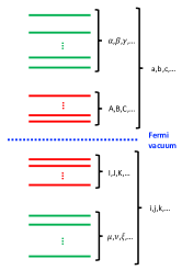
Figure 1: A schematic representation of the partitioning of the spinorbital domain into occupied inactive ($\mu$,$\nu$,$\xi$,$\ldots$), occupied active ($I$, $J$, $K$, $\ldots$), virtual active ($A$, $B$, $C$, $\ldots$), and virtual inactive ($\alpha$, $\beta$, $\gamma$, $\ldots$). Generic occupied and virtual are denoted as $i$, $j$, $k$, $\ldots$, and $a$, $b$, $c$, $\ldots$, respectively.

All Slater determinants spanning the external space can be partitioned into two disjoint sets of determinants $S_{1}=\{|\Phi_{\mathcal{O}(\mu)}^{\mathcal{V}}\rangle\}_{\mu=\mu_{1}}^{\mu_{F}}$ and $S_{2}=\{|\Phi_{\mathcal{O_{\rm act}}}^{\mathcal{V}(\alpha)}\rangle\}$, where $\mathcal{O}(\mu)$ and $\mathcal{V}(\alpha)$ designate ordered string containing at least one inactive occupied ($\mu$) and inactive virtual ($\alpha$) index, respectively, and $\mathcal{O}_{\rm act}$ represents strings of occupied active indices only.

For the purpose of demonstrating the exactness of expansion (23), we will perform three classes of sweeps:
Sweep 1. We perform rotations to suppress all external excitatons containing at least one occupied inactive index according to the flow:

$$\displaystyle\mathop{\forall}_{a}|\Phi_{\mu_{1}}^{a}\rangle \rightarrow \displaystyle\mathop{\forall}_{i,a,b}|\Phi_{\mu_{1}i}^{ab}\rangle\rightarrow\displaystyle\mathop{\forall}_{i,j,a,b,c}|\Phi_{\mu_{1}ij}^{abc}\rangle\rightarrow\ldots$$

$$\displaystyle\mathop{\forall}_{a}|\Phi_{\mu_{2}}^{a}\rangle \rightarrow \displaystyle\mathop{\forall}_{i,a,b}|\Phi_{\mu_{2}i}^{ab}\rangle\rightarrow\displaystyle\mathop{\forall}_{i,j,a,b,c}|\Phi_{\mu_{2}ij}^{abc}\rangle\rightarrow\ldots\;,$$

$$\ldots \ldots$$

$$\displaystyle\mathop{\forall}_{a}|\Phi_{\mu_{F}}^{a}\rangle \rightarrow \displaystyle\mathop{\forall}_{i,a,b}|\Phi_{\mu_{F}i}^{ab}\rangle\rightarrow\displaystyle\mathop{\forall}_{i,j,a,b,c}|\Phi_{\mu_{F}ij}^{abc}\rangle\rightarrow\ldots\;,$$ (29)

where each step is given by basic unitary transformation (26). In this way, through applying a finite product of elementary unitary transformations

$$\Omega_{1}=\prod_{\mu=\mu_{F}}^{\mu_{1}}\prod_{K_{\mu}}{\rm exp}\{\gamma^{\mathcal{O}(K_{\mu})}_{\mathcal{V}(K_{\mu})}(E^{\mathcal{V}(K_{\mu})}_{\mathcal{O}(K_{\mu})}-E_{\mathcal{V}(K_{\mu})}^{\mathcal{O}(K_{\mu})})\}$$ (30)

where all $\gamma^{\mathcal{O}(K_{\mu})}_{\mathcal{V}(K_{\mu})}$ are external excitations. In other words, in $\Omega_{1}|\Psi\rangle$ all determinants belonging to $S_{1}$ have been eliminated. This step is identical with the first $\mu_{F}$ steps of the original algorithms if the ordering of occupied orbitals is the same.
Sweep 2. In the second step, we perform elimination of Slater determinants in set $S_{2}$. This can be achieved by the following sequence of elimination steps involving basic unitary transformations:

$$\displaystyle\mathop{\forall}_{\alpha}|\Phi_{I_{1}}^{\alpha}\rangle \rightarrow \displaystyle\mathop{\forall}_{I^{\prime},\alpha,b}|\Phi_{I_{1}I^{\prime}}^{[\alpha b]}\rangle\rightarrow\displaystyle\mathop{\forall}_{I^{\prime},I^{\prime\prime},\alpha,b,c}|\Phi_{I_{1}I^{\prime}I^{\prime\prime}}^{[\alpha bc]}\rangle\rightarrow\ldots$$

$$\displaystyle\mathop{\forall}_{\alpha}|\Phi_{I_{2}}^{\alpha}\rangle \rightarrow \displaystyle\mathop{\forall}_{I^{\prime},\alpha,b}|\Phi_{I_{2}I^{\prime}}^{[\alpha b]}\rangle\rightarrow\displaystyle\mathop{\forall}_{I^{\prime},I^{\prime\prime},\alpha,b,c}|\Phi_{I_{2}I^{\prime}I^{\prime\prime}}^{[\alpha bc]}\rangle\rightarrow\ldots$$

$$\ldots \ldots$$

$$\displaystyle\mathop{\forall}_{\alpha}|\Phi_{I_{F}}^{\alpha}\rangle$$ (31)

where $I_{k},I^{\prime},I^{\prime\prime},\ldots$ corresponds to the ordered strings $\{I_{k}I^{\prime}I^{\prime\prime}\ldots\}$, and $[\alpha bc\ldots]$ corresponds to ordered strings containing elements $\alpha,b,c,\ldots$ (for example, if $\alpha<b$ then $[\alpha b]$ corresponds to $\{\alpha b\}$ otherwise to $\{b\alpha\}$). The last step in (31) corresponds to zeroing coefficients only by single $|\Phi_{I_{F}}^{a}\rangle$ - since $I_{F}$ is the highest index of active occupied spinorbitals all other configurations (for example $|\Phi_{I_{F}I^{\prime}}^{[\alpha b]}\rangle$) were eliminated in earlier steps ($|\Phi_{I^{\prime}I_{F}}^{[\alpha b]}\rangle$). Sweep 2 corresponds to the following product of elementary unitary operations

$$\Omega_{2}=\prod_{I=I_{F}}^{I_{1}}\prod_{K_{I}}{\rm exp}\{\gamma^{O_{\rm act}(K_{I})}_{V_{\alpha}(K_{I})}(E_{O_{\rm act}(K_{I})}^{V_{\alpha}(K_{I})}-E^{O_{\rm act}(K_{I})}_{V_{\alpha}(K_{I})})\}\;,$$ (32)

where string $V_{\alpha}(K_{I})$ must contain at least one inactive virtual orbital $\alpha$. As in Sweep 1, all amplitudes $\gamma^{O_{\rm act}(K_{I})}_{V_{\alpha}(K_{I})}$ are of the external type. After the Sweep 2 only surviving Slater determinants in $\Omega_{2}\Omega_{1}|\Psi\rangle$ belong to the active space, i.e.,

$$\Omega_{2}\Omega_{1}|\Psi\rangle=|\Psi_{\rm act}\rangle=(P+Q_{\rm int})|\Psi_{\rm act}\rangle\;.$$ (33)

This reduction of $|\Psi\rangle$ has been achieved with the external excitations only.
Sweep 3. Repeating the reduction procedure for $|\Psi_{\rm act}\rangle$ in active spinorbital space we can write

$$\Omega_{3}|\Psi_{\rm act}\rangle=|\Phi\rangle\;,$$ (34)

where $\Omega_{3}$ involves rotations expressed in terms of internal excitations only

$$\Omega_{3}=\prod_{I=I_{F}}^{I_{1}}\prod_{K_{I}}{\rm exp}\{\gamma^{O_{\rm act}(K_{I})}_{V_{\rm act}(K_{I})}(E_{O_{\rm act}(K_{I})}^{V_{\rm act}(K_{I})}-E^{O_{\rm act}(K_{I})}_{V_{\rm act}(K_{I})})\}\;,$$ (35)

Summarizing, Sweeps 1-3 we can write

$$|\Psi\rangle=\Omega_{1}^{-1}\Omega_{2}^{-1}\Omega_{3}^{-1}|\Phi\rangle\;,$$ (36)

where $\Omega_{1}$ and $\Omega_{2}$ depends on the external excitations while $\Omega_{3}$ involves internal excitations only (i.e., $\Omega_{1}=\Omega_{1}(\gamma_{\rm ext})$, $\Omega_{2}=\Omega_{2}(\gamma_{\rm ext})$, $\Omega_{3}=\Omega_{3}(\gamma_{\rm int})$). Applying multiple times Baker-Campbell-Hausdorff (BCH) formula

$$e^{X}e^{Y}=e^{X+Y+\frac{1}{2}[X,Y]+\frac{1}{12}[X,[X,Y]]-\frac{1}{12}[Y,[X,Y]]+\ldots}$$ (37)

to $\Omega_{3}(\gamma_{\rm int})^{-1}$ and to the product of $\Omega_{1}(\gamma_{\rm ext})^{-1}\Omega_{2}(\gamma_{\rm ext})^{-1}$ one obtains

$$\Omega_{1}(\gamma_{\rm ext})^{-1}\Omega_{2}(\gamma_{\rm ext})^{-1} = e^{-\gamma_{\rm ext}+C_{12}(\gamma_{\rm ext})}$$ (38)

$$\Omega_{3}(\gamma_{\rm int})^{-1} = e^{\rm-\gamma_{\rm int}+C_{3}(\gamma_{\rm int})}$$ (39)

where $\gamma_{\rm ext}$ is a sum of external-type terms $\gamma^{\mathcal{O}}_{\mathcal{V}}(E^{\mathcal{V}}_{\mathcal{O}}-E^{\mathcal{O}}_{\mathcal{V}})$ defined in Sweeps 1 and 2 (see Eqs.(30) and (32)) and $\gamma_{\rm int}$ is a sum of internal-type terms defined in Sweep 3 (Eq.35). The $C_{12}(\gamma_{\rm ext})$ and $C_{3}(\gamma_{\rm int})$ are multiply-nested commutator expressions stemming from the multiple use of BCH expansion. Since $\gamma_{\rm ext}$ and $\gamma_{\rm int}$ are anti-Hermitian and the commutator of two anti-Hermitian operators is also anti-Hermitian. Therefore, we can represent the exact wave function in the form of product of the two unitary CC expansions involving external and internal degrees of freedom

$$|\Psi\rangle=e^{\sigma_{\rm ext}}e^{\sigma_{\rm int}}|\Phi\rangle$$ (40)

where general-type anti-Hermitian external and internal operators $\sigma_{\rm ext}$ and $\sigma_{\rm int}$ are given by the expressions

$$\sigma_{\rm ext} = -\gamma_{\rm ext}+C_{12}(\gamma_{\rm ext})\;,$$ (41)

$$\sigma_{\rm int} = -\gamma_{\rm int}+C_{3}(\gamma_{\rm int})\;.$$ (42)

Our following analysis will rely on the exactness of this expansion. If we change the parametrization

$$\gamma_{\rm ext} = -(T_{\rm ext}-T_{\rm ext}^{\dagger})\;,$$ (43)

$$\gamma_{\rm int} = -(T_{\rm int}-T_{\rm int}^{\dagger})\;,$$ (44)

where $T_{\rm ext}$ and $T_{\rm int}$ operators are characterized by the same many-body structure as in the SESCC case (14), then

$$\sigma_{\rm ext} = T_{\rm ext}-T_{\rm ext}^{\dagger}+C_{12}(T_{\rm ext},T_{\rm ext}^{\dagger})\;,$$ (45)

$$\sigma_{\rm int} = T_{\rm int}-T_{\rm int}^{\dagger}+C_{3}(T_{\rm int},T_{\rm int}^{\dagger})\;.$$ (46)

Using the same arguments as in Ref.Bauman et al. (2019a) one can easily show that the exact DUCC expansion (40) allows effective Hamiltonians to be constructed in a similar way as in single reference SESCC. It can be proven that both the exact energy and the $e^{\sigma_{\rm int}}|\Phi\rangle$ FCI CAS state can be obtained by diagonalizing the DUCC effective Hamiltonian in the complete active space

$$H^{\rm eff}e^{\sigma_{\rm int}}|\Phi\rangle=Ee^{\sigma_{\rm int}}|\Phi\rangle,$$ (47)

where

$$H^{\rm eff}=(P+Q_{\rm int})\bar{H}_{\rm ext}(P+Q_{\rm int})$$ (48)

and

$$\bar{H}_{\rm ext}=e^{-\sigma_{\rm ext}}He^{\sigma_{\rm ext}}.$$ (49)

In the construction of the DUCC effective Hamiltonian, only the external cluster operator ($\sigma_{\rm ext}$) is used. In further analysis, for both SESCC and DUCC formalisms we will use the same notation for the $\bar{H}_{\rm ext}$ and $H^{\rm eff}$ operators, and their form will follow from the context of the discussed equations, depending on if $T_{\rm ext}$, $\sigma_{\rm ext}$, or their analogous time-dependent variants $T_{\rm ext}(t)$ and $\sigma_{\rm ext}(t)$ are utilized.

The above analysis is predicated on the assumption that the infinite summations defining $\sigma_{\rm int}$ and $\sigma_{\rm ext}$ operators (given by Eqs.(45) and (46)) are convergent. For strongly correlated regime, where for example, amplitudes defining $T_{\rm int}$ are large, one can expect possible problems associated with the convergence of expansion (46). However, there are classes of applications such as the Quantum Phase Estimaton (QPE) algorithm in quantum computing,Luis and Peřina (1996); Cleve et al. (1998); Berry et al. (2007); Childs (2010); Wecker et al. (2015); Häner et al. (2016); Poulin et al. (2017) where $\sigma_{\rm int}$’s explicit construction is not required. Instead, the QPE algorithm utilizes information about $H^{\rm eff}$, which depends only on the $\sigma_{\rm ext}$ operator. By the proper choice of the active space, which should be large enough to make numerical values of $T_{\rm ext}$ sufficiently small, we can assume that the expansion (45) is convergent. In the following sections, we will also discuss other formulations (especially in the context of imaginary time evolution) where $e^{\sigma_{\rm int}}|\Phi\rangle$ Ansatz in the active space can be formally replaced by other exact expansions in the same active space.

A legitimate approximation of $\sigma_{\rm ext}$ and $\sigma_{\rm int}$ in Eqs.(45) and (46)is to retain lowest-order terms only, i.e.,

$$\sigma_{\rm int} \simeq T_{\rm int}-T_{\rm int}^{\dagger}\;,$$ (50)

$$\sigma_{\rm ext} \simeq T_{\rm ext}-T_{\rm ext}^{\dagger}\;,$$ (51)

which has been discussed in Ref.Bauman et al. (2019a).

III Time-dependent formulations employing downfolded Hamiltonians

To derive properties of the time-dependent Schrödinger equations utilizing SESCC and DUCC representations of the time-dependent wave functions, we will (in analogy to Refs.Schönhammer and Gunnarsson (1978); Huber and Klamroth (2011); Pigg et al. (2012) focus on the simplest case where orbitals and the reference function $|\Phi\rangle$ are time-independent, which can be expressed as

$$\frac{\partial}{\partial t}a_{p}=\frac{\partial}{\partial t}a_{q}^{\dagger}=0\;,\;\frac{\partial}{\partial t}|\Phi\rangle=0\;.$$ (52)

The above assumptions indicate that the CAS and corresponding SES $\mathfrak{h}$ do not change in time.

III.1 Time-dependent Schrödinger equation in the SESCC representation

In this subsection, we derive the time-dependent extension of the SESCC and DUCC wave function representations. First, we start from the time-dependent CC parametrization of the wave function:

$$|\Psi_{\rm CC}(t)\rangle=e^{T(t)}|\Phi\rangle\;,$$ (53)

where

$$T(t)=\sum_{k=0}^{m}T_{k}(t)\;.$$ (54)

As in the stationary SESCC formulation, we will assume the decomposition of the time-dependent cluster operator $T(t)$ into internal ($T_{\rm int}(t)$) and external ($T_{\rm ext}(t)$) parts, i.e,

$$|\Psi_{\rm CC}(t)\rangle = e^{T_{\rm ext}(t)+T_{\rm int}(t)}|\Phi\rangle$$ (55)

$$= e^{T_{\rm ext}(t)}e^{T_{\rm int}(t)}|\Phi\rangle\;.$$ (56)

For the sake of generality, we also include a time-dependent scalar phase factor ($T_{0}(t)$) in the definition of the $T_{\rm int}(t)$ operator. As pointed out by Hoodbhoy and Negele in Refs.Hoodbhoy and Negele (1978, 1979) this phase factor is not needed when calculating physical observables.

Upon introducing expansion (56) into the time-dependent Schrödinger equation, one obtains

$$i\hbar\frac{\partial}{\partial t}e^{T_{\rm ext}(t)}e^{T_{\rm int}(t)}|\Phi\rangle=He^{T_{\rm ext}(t)}e^{T_{\rm int}(t)}|\Phi\rangle\;,$$ (57)

which can be further transformed (after differentiating its left-hand side over $t$)

$$i\hbar(\frac{\partial T_{\rm int}(t)}{\partial t}+\frac{\partial T_{\rm ext}(t))}{\partial t})e^{T_{\rm ext}(t)}e^{T_{\rm int}(t)}|\Phi\rangle =$$ (58)

$$He^{T_{\rm ext}(t)}e^{T_{\rm int}(t)}|\Phi\rangle\;,$$

After pre-multiplying both sides by $e^{-T_{\rm ext}(t)}$, we obtain a convenient form of TDSE

$$i\hbar(\frac{\partial T_{\rm int}(t)}{\partial t}+\frac{\partial T_{\rm ext}(t)}{\partial t})e^{T_{\rm int}(t)}|\Phi\rangle =$$ (59)

$$\bar{H}_{\rm ext}(t)e^{T_{\rm int}(t)}|\Phi\rangle\;,$$

where

$$\bar{H}_{\rm ext}(t)=e^{-T_{\rm ext}(t)}He^{T_{\rm ext}(t)}\;.$$ (60)

Now, we focus our attention on the projection of Eq.(59) onto time-independent subspace $(P+Q_{\rm int})$, which leads to the equations:

$$i\hbar(P+Q_{\rm int})(\frac{\partial T_{\rm int}(t)}{\partial t}+\frac{\partial T_{\rm ext}(t)}{\partial t})e^{T_{\rm int}(t)}|\Phi\rangle$$

$$=(P+Q_{\rm int})\bar{H}_{\rm ext}(t)e^{T_{\rm int}(t)}|\Phi\rangle\;.$$ (61)

Taking into account the fact that $T_{\rm ext}(t)$ and $\frac{\partial}{\partial t}T_{\rm ext}(t)$ produce "external" excitations (defined by strings of creation-annihilation operators containing at least one inactive spin-orbital index) we have

$$(P+Q_{\rm int})\frac{\partial T_{\rm ext}(t)}{\partial t}e^{T_{\rm int}(t)}|\Phi\rangle=0$$ (62)

and therefore the time evolution of $e^{T_{\rm int}(t)}|\Phi\rangle$ corresponds to the non-unitary evolution in time-independent $(P+Q_{\rm int})$ space

$$i\hbar(P+Q_{\rm int})\frac{\partial T_{\rm int}(t)}{\partial t}e^{T_{\rm int}(t)}|\Phi\rangle=(P+Q_{\rm int})\bar{H}_{\rm ext}(t)e^{T_{\rm int}(t)}|\Phi\rangle$$ (63)

or

$$i\hbar\frac{\partial}{\partial t}e^{T_{\rm int}(t)}|\Phi\rangle=H^{\rm eff}(t)e^{T_{\rm int}(t)}|\Phi\rangle\;,$$ (64)

where we used the fact that

$$(P+Q_{\rm int})e^{T_{\rm int}(t)}|\Phi\rangle=e^{T_{\rm int}(t)}|\Phi\rangle$$ (65)

and

$$H^{\rm eff}(t)=(P+Q_{\rm int})\bar{H}_{\rm ext}(t)(P+Q_{\rm int})\;.$$ (66)

We will refer to equation (64) as embedded sub-system time evolution for the ket-state. In the above equations, we avoided the explicit operator notation $i\hbar\frac{\partial}{\partial t}T_{\rm int}(t)|\Phi\rangle=e^{-T_{\rm int}(t)}H^{\rm eff}(t)e^{T_{\rm int}(t)}|\Phi\rangle$ since the same notation is much harder to define in the DUCC case.

III.2 Time-dependent Schrödinger equation in the DUCC representation

The non-Hermitian character of $\bar{H}_{\rm ext}(t)$ may limit applications of this formalism in the area of quantum computing. In analogy to the DUCC formalism studied in Refs.Bauman et al. (2019a, b, 2020) let us represent normalized time-dependent wave function $|\Psi_{\rm DUCC}(t)\rangle$ in the following form

$$|\Psi_{\rm DUCC}(t)\rangle=e^{\sigma_{\rm ext}(t)}e^{\sigma_{\rm int}(t)}|\Phi\rangle\;,$$ (67)

where $\sigma_{\rm int}(t)$ and $\sigma_{\rm ext}(t)$ are general-type time-dependent anti-Hermitian operators in the sense of Eqs.(45) and (46), i.e.,

$$\sigma_{\rm int}(t)^{\dagger} = -\sigma_{\rm int}(t)\;,$$ (68)

$$\sigma_{\rm ext}(t)^{\dagger} = -\sigma_{\rm ext}(t)\;.$$ (69)

We also assume that the phase factor $i\delta$ is included in the definition of $\sigma_{\rm int}$. Introducing (67) into the TDSE leads to the equation

$$i\hbar(\frac{\partial e^{\sigma_{\rm ext}(t)}}{\partial t}e^{\sigma_{\rm int}(t)}+e^{\sigma_{\rm ext}(t)}\frac{\partial e^{\sigma_{\rm int}(t)}}{\partial t})|\Phi\rangle =$$ (70)

$$He^{\sigma_{\rm ext}(t)}e^{\sigma_{\rm int}(t)}|\Phi\rangle\;.$$

By pre-multiplying both sides of the above equation by $e^{-\sigma_{\rm ext}(t)}$ and projecting onto $(P+Q_{\rm int})$ subspace one obtains

$$i\hbar\frac{\partial e^{\sigma_{\rm int}(t)}}{\partial t}|\Phi\rangle=H^{\rm eff}(\sigma_{\rm ext}(t),\frac{\partial\sigma_{\rm ext}(t)}{\partial t})e^{\sigma_{\rm int}(t)}|\Phi\rangle\;,$$ (71)

where

$$H^{\rm eff}(\sigma_{\rm ext}(t),\frac{\partial\sigma_{\rm ext}(t)}{\partial t})=(P+Q_{\rm int})[\bar{H}_{\rm ext}-i\hbar e^{-\sigma_{\rm ext}(t)}\frac{\partial e^{\sigma_{\rm ext}(t)}}{\partial t}](P+Q_{\rm int})$$ (72)

and

$$\bar{H}_{\rm ext}(t)=e^{-\sigma_{\rm ext}(t)}He^{\sigma_{\rm ext}(t)}\;.$$ (73)

To analyze the many-body structure of the Hermitian effective Hamiltonian (72) we will use the following identity for calculating derivatives of exponential operators (see Refs.Rossmann (2006); Hall (2015) for more details)

$$\frac{\partial}{\partial t}e^{X(t)} = e^{X(t)}\sum_{k=0}^{\infty}\frac{(-1)^{k}}{(k+1)!}(ad_{X(t)})^{k}\frac{\partial X(t)}{\partial t}$$ (74)

$$= e^{X(t)}\sum_{k=0}^{\infty}\frac{(-1)^{k}}{(k+1)!}I_{k}(X(t),\frac{\partial X(t)}{\partial t})$$ (75)

where the adjoint action $ad_{X}$ is defined as

$$ad_{A}(B)=[A,B]\;$$ (76)

and $k$-commutator term $I_{k}(X(t),\frac{\partial X(t)}{\partial t})$ is given by the formula

$$I_{k}(X(t),\frac{\partial X(t)}{\partial t})=\underbrace{[X(t),[X(t),\ldots[X(t),[X(t),\frac{\partial X(t)}{\partial t}]]\ldots]]}_{k\;{\rm times}}\;.$$ (77)

It is easy to notice that the first terms in the expansion (75) are given by the expressions

$$I_{0}(X(t),\frac{\partial X(t)}{\partial t}) = \frac{\partial X(t)}{\partial t}\;,$$ (78)

$$I_{1}(X(t),\frac{\partial X(t)}{\partial t}) = [X(t),\frac{\partial X(t)}{\partial t}]\;,$$ (79)

and for $k\geq 1$ recursive formula is satisfied

$$I_{k}=[X(t),I_{k-1}(t)]\;.$$ (80)

Henceforth, for the simplicity of notation, we will use $I_{k}$ and $I_{k}(X(t),\frac{\partial X(t)}{\partial t})$ interchangeably.

Formula (75) will be used to evaluate the

$$\frac{\partial e^{\sigma_{\rm ext}(t)}}{\partial t}$$ (81)

term in Eq.(72), which using formula (75) can be re-written in the form:

$$e^{\sigma_{\rm ext}(t)}A(\sigma_{\rm ext}(t),\frac{\partial\sigma_{\rm ext}(t)}{\partial t})$$ (82)

where

$$A(\sigma_{\rm ext}(t),\frac{\partial\sigma_{\rm ext}(t)}{\partial t})=\sum_{k=0}^{\infty}\frac{(-1)^{k}}{(k+1)!}I_{k}(\sigma_{\rm ext}(t),\frac{\partial\sigma_{\rm ext}(t)}{\partial t})\;.$$ (83)

Given the fact that both $\sigma_{\rm ext}(t)$ and $\frac{\partial\sigma_{\rm ext}(t)}{\partial t}$ operators are anti-Hermitian, it is easy to show the same is true for $I_{k}(\sigma_{\rm ext}(t),\frac{\partial\sigma_{\rm ext}(t)}{\partial t})$ and $A(\sigma_{\rm ext}(t),\frac{\partial\sigma_{\rm ext}(t)}{\partial t})$ operators, i.e.,

$$I_{k}(\sigma_{\rm ext}(t),\frac{\partial\sigma_{\rm ext}(t)}{\partial t})^{\dagger} = -I_{k}(\sigma_{\rm ext}(t),\frac{\partial\sigma_{\rm ext}(t)}{\partial t})\;,$$ (84)

$$A(\sigma_{\rm ext}(t),\frac{\partial\sigma_{\rm ext}(t)}{\partial t})^{\dagger} = -A(\sigma_{\rm ext}(t),\frac{\partial\sigma_{\rm ext}(t)}{\partial t})\;.$$ (85)

Now, the effective (or downfolded) Hamiltonian (72) is given be the expression

$$H^{\rm eff}(\sigma_{\rm ext}(t),\frac{\partial\sigma_{\rm ext}(t)}{\partial t})=(P+Q_{\rm int})\{\bar{H}_{\rm ext}(t)-i\hbar A(\sigma_{\rm ext}(t),\frac{\partial\sigma_{\rm ext}(t)}{\partial t})\}(P+Q_{\rm int})\;.$$ (86)

In deriving the above equations, we employed the fact that

$$e^{\sigma_{\rm int}(t)}|\Phi\rangle=(P+Q_{\rm int})e^{\sigma_{\rm int}(t)}|\Phi\rangle\;.$$ (87)

III.3 Common features of TD-SESCC and TD-DUCC formulations

In previous subsections, we showed that when the orbital basis is time-independent then for both TD-SESCC and TD-DUCC cases the dynamics of the sub-system at the level of ket-state (defined by appropriately chosen SES $\mathfrak{h}$ or equivalently active space) can be described by the effective/downfolded Hamiltonians acting in the active space. While in the TD-SESCC case the dynamic is generated by a non-Hermitian Hamiltonian, for the TD-DUCC formalism, the downfolded Hamiltonian is Hermitian and contains "external-velocity" dependent term (i.e., $\frac{\partial\sigma_{\rm ext}(t)}{\partial t}$-dependent term - $A$ operator in Eq.(86)). In both cases at the level of the ket-state evolution, one can observe a rigorous decomposition of external Fermionic degrees of freedom ($T_{\rm ext}(t)$ and $\sigma_{\rm ext}(t)$ operators) from those defining sub-system time-dependent wave function ($T_{\rm int}(t)$ and $\sigma_{\rm int}(t)$) in the time-dependent downfolded Hamiltonian. By the appropriate choice of the active space, these approaches can be used to separate the description of the sub-system that slowly evolves in time (representing low-energy modes) from the components of the entire system that correspond to fast-varying components (representing high-energy modes) of the entire system. As suggested by earlier analysis (see Ref.Bauman et al. (2019a)) parameters corresponding to fast-varying parts can be effectively described by perturbation techniques. Simulations of these sub-systems can be performed employing explicit time-propagation techniques described in Refs.Schönhammer and Gunnarsson (1978); Hoodbhoy and Negele (1978, 1979); Huber and Klamroth (2011).

Although it has already been discussed in the literature (for example, see Ref.Kvaal (2012)) that to calculate expectation values of physical observables in the CC method, additional state parameters need to be introduced (in the case of the standard CC theory these parameters correspond to cluster operator $T$ and the so-called $\Lambda$ operator, where $\langle\Phi|(1+\Lambda)$ is the left eigenvector of the $\bar{H}$ operator), the above decomposition of the ket-variant of TDSE plays an important role for newly introduced equation-of-motion CC cumulant Green’s function theory Rehr et al. (2020) especially in the context of calculating spectral functions (see also Ref.Schönhammer and Gunnarsson (1978)) and reducing its numerical cost. However, to understand the advantages and limitations of the TD-SESCC and TD-DUCC formalisms in calculating physical observables, in the next section, we will analyze the properties of the corresponding action functionals.

IV Action functionals for TD-SESCC and TD-DUCC formulations

The form of optimal time evolution (or optimal equations of motion) for approximate theories describing time-dependent wavefunction $|\Psi\rangle$ can be determined by using the Dirac-Frenkel time-dependent variational principle (TDVP),Frenkel (1934); Kramer and Saraceno (1980) (for a detailed discussion see also Refs.Löwdin and Mukherjee (1972); Moccia (1973); Reinhard (1977); Kramer and Saraceno (1980); Meyer et al. (1990); Broeckhove et al. (1988); Goings et al. (2018)) where one varies the action integrals

$$\mathcal{S}[\Psi(t)]=\int_{t_{1}}^{t_{2}}\langle\Psi(t)|i\hbar\frac{\partial}{\partial t}-H|\Psi(t)\rangle dt\;.$$ (88)

to obtain the equations of motion for parameters describing time-dependent wave function. This functional has paved the wave for time-dependent formulations, including various variants of time-dependent multi-configurational methods.Meyer et al. (1990); Miranda et al. (2011); Hochstuhl and Bonitz (2012); Sato and Ishikawa (2013, 2015); Miyagi and Bojer Madsen (2014); Miyagi and Madsen (2014) In the above formulation, the normalization of the time-dependent wave function,

$$\langle\Psi(t)|\Psi(t)\rangle=1\;,$$ (89)

is assumed, which significantly simplifies the utilization of TDVP since for this type of domain the $i\hbar\frac{\partial}{\partial t}$ operator is the Hermitian operator and $\mathcal{S}[\Psi(t)]$ functional assumes real values. The Dirac-Frenkel functional has been extended to bi-variational CC formulations by Arponen Arponen (1983) (for original discussion of bi-variational formalism see Ref.Chernoff and Marsden (2006))

$$\mathcal{S}[\Psi(t),\Psi^{\prime}(t)]=\int_{t_{1}}^{t_{2}}\langle\Psi^{\prime}(t)|i\hbar\frac{\partial}{\partial t}-H|\Psi(t)\rangle dt\;.$$ (90)

where the trial wave functions $\langle\Psi^{\prime}(t)|$ and $|\Psi(t)\rangle$ satisfy the normalization condition

$$\langle\Psi^{\prime}(t)|\Psi(t)\rangle=1\;.$$ (91)

The analysis of the CC methods is greatly facilitated by using the Lagrangian (see Ref.Kramer and Saraceno (1980)) defined as

$$L(\Psi(t),\Psi^{\prime}(t))=\langle\Psi^{\prime}(t)|i\hbar\frac{\partial}{\partial t}-H|\Psi(t)\rangle\;,$$ (92)

and

$$\mathcal{S}[\Psi(t),\Psi^{\prime}(t)]=\int_{t_{1}}^{t_{2}}L(\Psi(t),\Psi^{\prime}(t))dt\;.$$ (93)

The Lagrangian (92), for simplicity denoted as $L(\Psi(t),\Psi^{\prime}(t))$, should be understood in a broader context not only as a function of $\langle\Psi^{\prime}(t)|$ and $|\Psi(t)\rangle$ states but also as a function of their time-derivatives. The Arponen’s functional provides a theoretical foundation, especially for time-dependent formulations of the coupled cluster theory. Recently, Kvaal and Pedersen used this functional to develop orbital adaptive time-dependent coupled cluster approximations Kvaal (2012) and symplectic integrators for TD-CC equations.Pedersen and Kvaal (2019) The real-action functional introduced by Sato et al. in studies of TD-CC theory also invokes the bi-orthogonal form of the Arponen’s functional.Sato et al. (2018) Both functionals (88) and (90) are very useful in situations where one also considers time evolution of reference function and molecular basis.

In this section, we will employ functionals (88) and (90) to study stationary conditions for TD-SESCC and TD-DUCC formulations, respectively, and to describe time evolution of sub-system described by the internal type excitations. The Lagrangian for normalized DUCC wave function takes the following form

$$L[\sigma_{\rm int}(t),\sigma_{\rm ext}(t)] =$$ (94)

$$\langle\Phi|e^{-\sigma_{\rm int}(t)}e^{-\sigma_{\rm ext}(t)}(i\hbar\frac{\partial}{\partial t}-H)e^{\sigma_{\rm ext}(t)}e^{\sigma_{\rm int}(t)}|\Phi\rangle$$

where, as stated earlier, we assume that one-particle orbital basis is time-independent. Since the DUCC wave function is normalized, the $S[\sigma_{\rm int}(t),\sigma_{\rm ext}(t)]$ assumes real values. In the next step, we will re-write functional (94) using results of the previous section (see Eqs. (75), (81), (82), (83))

$$i\hbar e^{-\sigma_{\rm ext}(t)}\frac{\partial}{\partial t}e^{\sigma_{\rm ext}(t)}=i\hbar\frac{\partial}{\partial t}+i\hbar A(\sigma_{\rm ext}(t),\frac{\partial\sigma_{\rm ext}(t)}{\partial t})\;,$$ (95)

which after substituting to Eq.(94) leads to the expression for the Lagrangian

$$L[\sigma_{\rm int}(t),\sigma_{\rm ext}(t)]=\langle\Phi|e^{-\sigma_{\rm int}(t)}\{i\hbar\frac{\partial}{\partial t}-[\bar{H}_{\rm ext}(t)-i\hbar A(\sigma_{\rm ext}(t),\frac{\partial\sigma_{\rm ext}(t)}{\partial t})]\}e^{\sigma_{\rm int}(t)}|\Phi\rangle\;.$$ (96)

The above expression can be represented in an equivalent form using (86) and (87)

$$L[\sigma_{\rm int}(t),\sigma_{\rm ext}(t)]=\langle\Phi|e^{-\sigma_{\rm int}(t)}\{i\hbar\frac{\partial}{\partial t}-H^{\rm eff}(\sigma_{\rm ext}(t),\frac{\partial\sigma_{\rm ext}(t)}{\partial t},t)\}e^{\sigma_{\rm int}(t)}|\Phi\rangle\;,$$ (97)

which can be interpreted in terms of slow- and fast-varying parts of the wave function represented in terms of $\sigma_{\rm int}(t)$ and $\sigma_{\rm ext}(t)$ operators if the "energetic" definition of the active space (or SES) is utilized. Namely, if the fast-varying in time part of the wave function (or $\sigma_{\rm ext}(t)$-dependent part of the wave function) is known or can be efficiently approximated then the slow-varying dynamic (captured by the proper choice of the active space and $\sigma_{\rm int}(t)$ operator) of the entire system can be described as a sub-system dynamics generated by the Hermitian $H^{\rm eff}(\sigma_{\rm ext}(t),\frac{\partial\sigma_{\rm ext}(t)}{\partial t})$ operator. This decoupling of various time regimes (slow- vs. fast-varying components) is analogous to the decoupling of high- and low-energy Fermionic degrees of freedom in stationary formulations of the SESCC and DUCC formalisms (see Refs.Bauman et al. (2019a, b)). This result indicates that there exist universal mechanisms in coupled cluster theory that naturally lead to the decoupling of various temporal, energy, and spatial scales as shown in present analysis and in Refs.Kowalski (2018); Bauman et al. (2019a).

Properties of the Arponen’s functional draw heavily on the representations of the bra and ket states. Here we will analyze the standard approach analyzed in references Arponen (1983); Kvaal (2012); Pigg et al. (2012); Sato et al. (2018); Pedersen and Kvaal (2019) where ket state is represented by standard CC expansion (3) while the bra is represented using a standard de-excitation $\Lambda(t)$ operator Arponen (1983)

$$\langle\Psi^{\prime}(t)|=\langle\Phi|(1+\Lambda(t))e^{-T(t)}$$ (98)

$$=\langle\Phi|(1+\Lambda_{\rm int}(t)+\Lambda_{\rm ext}(t))e^{-T_{\rm int}(t)}e^{-T_{\rm ext}(t)}\;,$$ (99)

which leads to the following form of the Lagrangian for the Arponen’s functional

$$L[\Lambda_{\rm int}(t),\Lambda_{\rm ext}(t),T_{\rm int}(t),T_{\rm ext}(t)]=\langle\Phi|(1+\Lambda_{\rm int}(t)+\Lambda_{\rm ext}(t))e^{-T_{\rm int}(t)}e^{-T_{\rm ext}(t)}(i\hbar\frac{\partial}{\partial t}-H)e^{T_{\rm ext}(t)}e^{T_{\rm int}(t)}|\Phi\rangle$$ (100)

$$=\langle\Phi|(1+\Lambda_{\rm int}(t))e^{-T_{\rm int}(t)}(i\hbar\frac{\partial}{\partial t}-\bar{H}_{\rm ext}(t))e^{T_{\rm int}(t)}|\Phi\rangle+\langle\Phi|\Lambda_{\rm ext}(t)e^{-T_{\rm int}(t)}(i\hbar\frac{\partial T_{\rm ext}(t)}{\partial t}+i\hbar\frac{\partial}{\partial t}-\bar{H}_{\rm ext})e^{T_{\rm int}(t)}|\Phi\rangle \;.$$ (101)

Comparing the above expression for the current functional with the DUCC one (97) leads to the observation that the DUCC functional can be expressed directly in terms of a sub-system perspective, where the dynamics for the sub-system is generated by $\bar{H}_{\rm ext}-i\hbar A$ whereas for the TD-SESCC case only the first term in Eq.(101) can be interpreted in a similar way. The remaining term in Eq.(101) introduces explicit coupling between $\Lambda_{\rm ext}(t)$ and $T_{\rm int}(t)$ operators and cannot be considered in terms of sub-system dynamics, as in the case of DUCC functional. This is a consequence of the fact that the state (98) is not multiplicatively separable. As mentioned earlier, the algebraic form and properties of Arponen’s functional depends on the parametrization used for the bra state $\langle\Psi^{\prime}(t)|$. In the appendix, we analyze the form of the Arponen’s functional where the extended coupled cluster (ECC) method Arponen (1983) is invoked to represent $\langle\Psi^{\prime}(t)|$ state (see also Ref.Kvaal et al. (2020) for recent developments of the time-dependent ECC formalism). We show that it is possible to derive a similar form of expressions as in the DUCC case. many-body structure.

V Imaginary time evolution generated by downfolded Hamiltonians

Due to the Hermitian character of the effective Hamiltonian and potential applications in quantum computing in this section we will focus entirely on the DUCC approach. In this section, we will focus on the stationary conditions for the $\sigma_{\rm int}(t)$ operator stemming from functional (96). Since the $e^{\sigma_{\rm int}(t)}|\Phi\rangle$ is an exact wave function in the complete active space, it can be equivalently represented by the active-space FCI expansion

$$|\Psi_{\rm int}(t)\rangle=e^{\sigma_{\rm int}(t)}|\Phi\rangle=C_{\rm int}(t)|\Phi\rangle\;,$$ (102)

where $C_{\rm int}(t)$ is the configuration interaction type operator that produces all possible excitations/configurations within CAS and which satisfies the normalization condition

$$\langle\Psi_{\rm int}(t)|\Psi_{\rm int}(t)\rangle=\langle\Phi|C_{\rm int}(t)^{\dagger}C_{\rm int}|\Phi\rangle=1\;.$$ (103)

In the $(C_{\rm int}(t),\sigma_{\rm ext}(t))$ parametrization, the Lagrangian (96) takes the form

$$L[C_{\rm int}(t),\sigma_{\rm ext}(t)]=\langle\Phi|C_{\rm int}(t)^{\dagger}\{i\hbar\frac{\partial}{\partial t}-[\bar{H}_{\rm ext}(t)-i\hbar A(\sigma_{\rm ext}(t),\frac{\partial\sigma_{\rm ext}(t)}{\partial t})]\}C_{\rm int}(t)|\Phi\rangle\;.$$ (104)

One should notice that there is no change in the algebraic form of the $\bar{H}_{\rm ext}(t)$ and $A(\sigma_{\rm ext}(t),\frac{\partial\sigma_{\rm ext}(t)}{\partial t})$ operators and stationary conditions for $C_{\rm int}(t)$ can be obtained following derivations for the TD-MCSCF and TD-CASSCF procedures of Refs.Miranda et al. (2011); Sato and Ishikawa (2013), i.e.,

$$i\hbar\frac{\partial C_{\rm int}(t)}{\partial t}|\Phi\rangle=H^{\rm eff}(\sigma_{\rm ext}(t),\frac{\partial\sigma_{\rm ext}(t)}{\partial t})C_{\rm int}(t)|\Phi\rangle\;,$$ (105)

where the $H^{\rm eff}(\sigma_{\rm ext}(t),\frac{\partial\sigma_{\rm ext}(t)}{\partial t})$ operator is given by Eq.(86). The above equations correspond to the equations (see Eq.(71)) defining dynamics of the $\sigma_{\rm int}(t)$ operator when returning to the $(\sigma_{\rm int}(t),\sigma_{\rm ext}(t))$ parametrization. Since exponential parametrization (which assures proper normalization of the sub-system wave function) is replaced by its linear representation, in numerical algorithms to solve (105) one needs to re-normalized $C_{\rm int}(t)|\Phi\rangle$ in each step using techniques of Refs.Kato and Kono (2004); Sato and Ishikawa (2013, 2015). In view of decoupling internal and external wave function parameters in the $H^{\rm eff}(\sigma_{\rm ext}(t),\frac{\partial\sigma_{\rm ext}(t)}{\partial t})$ operator a natural approximation is to use perturbative estimates of $\sigma_{\rm ext}(t)$ and describe evolution, of $C_{\rm int}(t)|\Phi\rangle$ or $e^{\sigma_{\rm int}(t)}|\Phi\rangle$ (Eq.(105) or (71)) using modified TD-MCSCF or TD-CASSCF implementations. Meyer et al. (1990); Miranda et al. (2011); Sato and Ishikawa (2013); Miyagi and Bojer Madsen (2014) In these simulations, the time-dependent $H^{\rm eff}(\sigma_{\rm ext}(t),\frac{\partial\sigma_{\rm ext}(t)}{\partial t})$ operator is used to generate the sub-system dynamics, which can be employed for example in studies of decoherence effects in open-systems. This can be achieved by analyzing density matrix corresponding to $C_{\rm int}|\Phi\rangle$ wave function.

In order to discuss imaginary time evolution based on the utilization of effective Hamiltonians we introduce imaginary Wick rotation $t\rightarrow-i\hbar\tau$. However, to take care of proper normalization of the $C_{\rm int}(\tau)|\Phi\rangle$ expansion in the $\tau\rightarrow\infty$ limit, one has to introduce appropriate renormalization term (or the so-called energy shift). Similar procedures are used in the context of other methods based on the imaginary-time Schrödinger equation, for example stochastic FCI methods, Booth et al. (2009) and recent formulations of quantum imaginary time evolution.McArdle et al. (2019) To define the equations for $C_{\rm int}(\tau)$ one can consider a steepest-descent flow for energy expectation value for normalized $C_{\rm int}(\tau)|\Phi\rangle$ function and effective Hamiltonian. This procedure leads to the following equations:

$$\frac{\partial C_{\rm int}(\tau)}{\partial\tau}|\Phi\rangle=-(H^{\rm eff}(\sigma_{\rm ext}(\tau),\frac{\partial\sigma_{\rm ext}(\tau)}{\partial\tau})-S(\tau))C_{\rm int}(\tau)|\Phi\rangle\;,$$ (106)

where the energy shift $S(\tau)$ is defined as a value of the energy functional constructed for $H^{\rm eff}(\sigma_{\rm ext}(\tau),\frac{\partial\sigma_{\rm ext}(\tau)}{\partial\tau})$ and properly normalized $C_{\rm int}(\tau)|\Phi\rangle$ trial function. Assuming that this approximation reaches the stationary limit (SL) for $\tau\rightarrow\infty$ (i.e. $\frac{\partial C_{\rm int}(\tau)}{\partial\tau}=0$, $\frac{\partial\sigma_{\rm ext}(\tau)}{\partial\tau}=0$) and

$$\sigma_{\rm ext}(\tau) \xrightarrow{SL} \sigma_{\rm ext}\;,$$ (107)

then the form of Eq.(106) for large values of $\tau$ is given by a simpler form

$$\frac{\partial C_{\rm int}(\tau)}{\partial\tau}|\Phi\rangle=-(P+Q_{\rm int})(\bar{H}_{\rm ext}(\sigma_{\rm ext}(\tau)))-\bar{S}(\tau))(P+Q_{\rm int})C_{\rm int}(\tau)|\Phi\rangle\;,$$ (108)

where $\bar{S}(\tau)$ is a value of energy functional defined by the $(P+Q_{\rm int})(\bar{H}_{\rm ext}(\sigma_{\rm ext}(\tau))(P+Q_{\rm int})$ operator and normalized $C_{\rm int}(\tau)|\Phi\rangle$ trial function. This step is a consequence of the fact that the "external-velocity" dependent term (i.e. $\frac{\partial\sigma_{\rm ext}(\tau)}{\partial\tau}$-dependent term - the $A$ operator in Eq.(83)) disappears in the SL limit, i.e.,

$$A(\sigma_{\rm ext}(\tau),\frac{\partial\sigma_{\rm ext}(\tau)}{\partial\tau}) \xrightarrow{SL} 0\;.$$ (109)

This important result is intuitively in agreement with the DUCC analysis discussed in previous papers Bauman et al. (2019a, b, 2020) where it was shown that the energy of the system can be obtained by diagonalizing stationary $\bar{H}_{\rm ext}$ Hamiltonian in the active space. Additionally, $\bar{H}_{\rm ext}(\sigma_{\rm ext}(\tau))$ is a similarity transformed Hamiltonian $H$ which is bounded from below. Projecting this Hamiltonian on a $(P+Q_{\rm int})$ subspace produces a downfolded Hamiltonian, which is bounded from below. This analysis shows the feasibility of imaginary time evolution in the TD-DUCC case. Additionally, since in the SL $\bar{H}_{\rm ext}(\sigma_{\rm ext}(\tau))$ approaches $\bar{H}_{\rm ext}$, to get the ground state energy one can alternatively perform imaginary evolutions with the fixed-in-time Hamiltonian $\bar{H}_{\rm ext}$ in the active space.

VI Conclusions

In this paper, we analyzed the extension of time-independent SESCC and DUCC formalisms to the time domain. We also proved the exactness of the double unitary CC Ansatz based on the general-type anti-Hermitian internal and external cluster operators. For a fixed-in-time orbital basis, we were able to prove that it is possible to describe the dynamics of the entire system for the ket states in terms of sub-system dynamics generated by a downfolded Hamiltonian. This feature, in the case of the SESCC formulation provides a way for reducing the numerical cost of CC Green’s function formulations. For the DUCC and ECC approaches we also showed the dynamic separability at the level of action functional, which is especially important from the point of view of constructing approximate formalisms. If the active space separates slow modes from the fast ones, perturbative techniques can be used to define downfolded Hamiltonians. In this paper, we put special emphasis on the TD-DUCC formalism where the operators defining the sub-system dynamics are Hermitian. Recognizing that if the $\sigma_{\rm ext}(\tau)$ operator reaches the stationary limit, then the time-dependent Hamiltonian converges to the time-independent downfolded Hamiltonian, demonstrating the feasibility of imaginary time evolution. In the stationary limit, the $A$ operator, which depends linearly on the $\sigma_{\rm ext}(t)$-velocity term, disappears, enabling the utilization of the time-dependent CASSCF codes to describe system dynamics in the time domain captured by the specific choice of the active space. Additionally, these results allow quantum Lanczos algorithms to be employed to identify the ground-state energy values.Motta et al. (2020) It is also interesting to look at the sub-system dynamics from the point of view of description decoherence effects, where the sub-system of interest is in contact with the surrounding environment described by the $\bar{H}^{\rm eff}(t)$ operator. In this paper, we cannot cover all aspects of the dynamics separation. Therefore in the following papers, we will study related topics such as time evolution of extensive observables, ECC formalisms, and DUCC approximate approaches for classical and quantum computing.

VII Data Availability Statement

The data that support the findings of this study are available from the corresponding author upon reasonable request.

VIII Acknowledgement

This work was supported by the "Embedding Quantum Computing into Many-body Frameworks for Strongly Correlated Molecular and Materials Systems" project, which is funded by the U.S. Department of Energy(DOE), Office of Science, Office of Basic Energy Sciences, the Division of Chemical Sciences, Geosciences, and Biosciences. All calculations have been performed using computational resources at the Pacific Northwest National Laboratory (PNNL). PNNL is operated for the U.S. Department of Energy by the Battelle Memorial Institute under Contract DE-AC06-76RLO-1830.

Appendix A Sub-system dynamics with extended coupled cluster formalism

As a specific example of the SESCC Arponen’s functional, we will focus on the bi-orthogonal formulation of TDVP given by the extended coupled cluster formalism where bra and ket trial states $\langle\Psi^{\prime}(t)|$ and $|\Psi(t)\rangle$ are parametrized as

$$\langle\Psi^{\prime}(t)| = \langle\Phi|e^{X(t)}e^{-T(t)}\;,$$ (110)

$$|\Psi(t)\rangle = e^{T(t)}|\Phi\rangle\;,$$ (111)

where $T(t)$ and $X(t)$ are standard excitation and de-excitation operators. Expressions (110) and (111) for trial wave function automatically satisfies normalization condition (91) and the functional (90) can be viewed as a function of cluster amplitudes defining $T(t)$ and $X(t)$ cluster operators

$$\mathcal{S}[T(t),X(t)]=\int_{t_{1}}^{t_{2}}\langle\Phi|e^{X(t)}e^{-T(t)}(i\hbar\frac{\partial}{\partial t}-H)e^{T(t)}|\Phi\rangle dt\;.$$ (112)

The stationary conditions provide equations of motion for the cluster amplitudes $T(t)$ and $X(t)$. Moreover, partial integration of (112) is required to obtain equations of motion for the $X(t)$ operator.

In analogy to standard excitation operator $T$, we will partition the de-excitation operator into its internal and external components (now the notion of sub-system embedding excitations should be replaced by the sub-system embedding de-excitations)

$$X(t)=X_{\rm int}(t)+X_{\rm ext}(t)$$ (113)

where all strings of de-excitation operators defining $X_{\rm int}(t)$ contain active spin-orbital indices only. The Arponen’s functional for the ECC formalism takes the form

$$\mathcal{S}[T_{\rm int}(t),T_{\rm ext}(t),X_{\rm int}(t),X_{\rm ext}(t)]=$$

$$\int_{t_{1}}^{t_{2}}\langle\Phi|e^{X_{\rm int}(t)}e^{X_{\rm ext}(t)}e^{-T_{\rm int}(t)}e^{-T_{\rm ext}(t)}(i\hbar\frac{\partial}{\partial t}-H)e^{T_{\rm ext}(t)}e^{T_{\rm int}(t)}|\Phi\rangle dt\;,$$ (114)

which is composed of time derivative $\mathcal{S}_{Dt}[T_{\rm int}(t),T_{\rm ext}(t),X_{\rm int}(t),X_{\rm ext}(t)]$ part and energy term $\mathcal{S}_{H}[T_{\rm int}(t),T_{\rm ext}(t),X_{\rm int}(t),X_{\rm ext}(t)]$ ($\mathcal{S}=\mathcal{S}_{Dt}+\mathcal{S}_{H}$). To define sub-system dynamics let us re-write $\mathcal{S}_{Dt}$ and $\mathcal{S}_{H}$ energy functional terms of (114) with Lagrangians ($L_{Dt}$ and $L_{H}$, $\mathcal{S}=\int_{t_{1}}^{t_{2}}(L_{Dt}(t)+L_{H}(t))dt$). For $L_{Dt}(t)$ we have

$$L_{Dt}(t) = \langle\Phi|e^{X_{\rm int}(t)}e^{X_{\rm ext}(t)}e^{-T_{\rm int}(t)}e^{-T_{\rm ext}(t)}(i\hbar\frac{\partial}{\partial t})e^{T_{\rm ext}(t)}e^{T_{\rm int}(t)}|\Phi\rangle$$ (115)

$$= i\hbar\langle\Phi|e^{X_{\rm int}(t)}e^{X_{\rm ext}(t)}\frac{\partial T_{\rm ext}(t)}{\partial t}|\Phi\rangle+\langle\Phi|e^{X_{\rm int}(t)}e^{-T_{\rm int}(t)}(i\hbar\frac{\partial}{\partial t})e^{T_{\rm int}(t)}|\Phi\rangle$$ (116)

$$= i\hbar\langle\Phi|e^{X_{\rm int}(t)}e^{-T_{\rm int}(t)}e^{T_{\rm int}(t)}(e^{X_{\rm ext}(t)}\frac{\partial T_{\rm ext}(t)}{\partial t})_{C}e^{-T_{\rm int}(t)}e^{T_{\rm int}(t)}|\Phi\rangle+\langle\Phi|e^{X_{\rm int}(t)}e^{-T_{\rm int}(t)}(i\hbar\frac{\partial}{\partial t})e^{T_{\rm int}(t)}|\Phi\rangle$$ (117)

$$= i\hbar\langle\Phi|e^{X_{\rm int}(t)}e^{-T_{\rm int}(t)}B(T_{\rm int}(t),\frac{\partial T_{\rm ext}(t)}{\partial t},X_{\rm ext}(t))e^{T_{\rm int}(t)}|\Phi\rangle+\langle\Phi|e^{X_{\rm int}(t)}e^{-T_{\rm int}(t)}(i\hbar\frac{\partial}{\partial t})e^{T_{\rm int}(t)}|\Phi\rangle$$ (118)

where $B(T_{\rm int}(t),\frac{\partial T_{\rm ext}(t)}{\partial t},X_{\rm ext}(t))$ (or $B$ term for short) is given by the formula

$$B=e^{T_{\rm int}(t)}(e^{X_{\rm ext}(t)}\frac{\partial T_{\rm ext}(t)}{\partial t})_{C}e^{-T_{\rm int}(t)}\;.$$ (119)

The connected character of the $e^{X_{\rm ext}(t)}\frac{\partial T_{\rm ext}(t)}{\partial t}$ expression in the first term on the right-hand side of Eq.(117) stems from the fact that in Eq.(116) the $e^{X_{\rm ext}(t)}\frac{\partial T_{\rm ext}(t)}{\partial t}$ operator is bracketed by two states belonging to the active space, i.e., $\langle\Phi|e^{X_{\rm int}(t)}$ and $|\Phi\rangle$, therefore for $e^{X_{\rm ext}(t)}\frac{\partial T_{\rm ext}(t)}{\partial t}$ to produce non-zero contributions all inactive lines have to be contracted out and all external lines of the resulting diagrams have to be active (see Fig.2). Consequently, only the active-space part of the $B$ operator produces a non-zero contribution to Eq.(118).

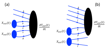
Figure 2: Examples of connected (a) and disconnected (b) diagrams contributing to $e^{X_{\rm ext}(t)}\frac{\partial T_{\rm ext}(t)}{\partial t}$. While the former diagram may result in a non-zero contributions to the first term on the right-hand side of (116) the latter one gives zero contribution.

Using similar manipulations, the $L_{H}(t)$ term can be re-written as

$$L_{H}(t) = \langle\Phi|e^{X_{\rm int}(t)}e^{X_{\rm ext}(t)}e^{-T_{\rm int}(t)}e^{-T_{\rm ext}(t)}He^{T_{\rm ext}(t)}e^{T_{\rm int}(t)}|\Phi\rangle$$ (120)

$$= \langle\Phi|e^{X_{\rm int}(t)}e^{-T_{\rm int}(t)}\bar{H}_{ECC}e^{T_{\rm int}(t)}|\Phi\rangle$$ (121)

where

$$\bar{H}_{\rm ECC}=e^{X^{\rm int}_{\rm ext}(t)}e^{-T_{\rm ext}(t)}He^{T_{\rm ext}(t)}e^{-X^{\rm int}_{\rm ext}(t)}$$ (122)

and

$$X^{\rm int}_{\rm ext}(t)=e^{T_{\rm int}(t)}X_{\rm ext}(t)e^{-T_{\rm int}(t)}$$ (123)

is a similarity transformed $X_{\rm ext}(t)$ operator. One should also notice that the above definition for the $X^{\rm int}_{\rm ext}(t)$ operator assures its connected character.

Summarizing, the $\mathcal{S}=\int_{t_{1}}^{t_{2}}(L_{Dt}(t)+L_{H}(t))dt$ functional can be expressed as:

$$\mathcal{S}=\int_{t_{1}}^{t_{2}}\langle\Phi|e^{X_{\rm int}(t)}e^{-T_{\rm int}(t)}\{i\hbar\frac{\partial}{\partial t}-[\bar{H}_{\rm ECC}(t)-i\hbar B(t)]\}e^{T_{\rm int}(t)}|\Phi\rangle\;.$$ (124)

Although the above formula bears a resemblance to functional (96), by their definitions $\bar{H}_{\rm ECC}(t)$ and $B(t)$ mix internal and external Fermionic degrees of freedom, in contrast to the DUCC functional (96). Another important feature of the ECC formalism is the fact that $\bar{H}_{\rm ECC}(t)$, as given by Eq.(122), is defined by rather complicated algebraic many-body structure defined by two similarity transformations one involving singly-transformed auxiliary operator $X^{\rm int}_{\rm ext}(t)$. Efficient coding of these expressions may require sophisticated symbolic algebra tools. This effort can be further facilitated by the utilization of the so-called doubly linked structure of resulting diagrams (see Ref.Arponen et al. (1987))

References

- Coester (1958) F. Coester, Nucl. Phys. 7, 421 (1958).
- Coester and Kümmel (1960) F. Coester and H. Kümmel, Nucl. Phys. 17, 477 (1960).
- Čížek (1966) J. Čížek, J. Chem. Phys. 45, 4256 (1966).
- Paldus et al. (1972) J. Paldus, J. Čížek, and I. Shavitt, Phys. Rev. A 5, 50 (1972).
- Purvis and Bartlett (1982) G. D. Purvis and R. J. Bartlett, J. Chem. Phys. 76, 1910 (1982).
- Paldus and Li (1999a) J. Paldus and X. Li, Adv. Chem. Phys. 110, 1 (1999a).
- Bartlett and Musiał (2007) R. J. Bartlett and M. Musiał, Rev. Mod. Phys. 79, 291 (2007).
- Hagen and Papenbrock (2019) G. Hagen and T. Papenbrock, Nature 569, 49 (2019).
- Monkhorst (1977) H. J. Monkhorst, Int. J. Quantum Chem. 12, 421 (1977).
- Koch and Jørgensen (1990) H. Koch and P. Jørgensen, J. Chem. Phys. 93, 3333 (1990).
- Geertsen et al. (1989) J. Geertsen, M. Rittby, and R. J. Bartlett, Chem. Phys. Lett. 164, 57 (1989).
- Comeau and Bartlett (1993) D. C. Comeau and R. J. Bartlett, Chem. Phys. Lett. 207, 414 (1993).
- Stanton and Bartlett (1993) J. F. Stanton and R. J. Bartlett, J. Chem. Phys. 98, 7029 (1993).
- Piecuch and Bartlett (1999) P. Piecuch and R. J. Bartlett, “Eomxcc: A new coupled-cluster method for electronic excited states,” (Academic Press, 1999) pp. 295–380.
- Mukherjee et al. (1977) D. Mukherjee, R. K. Moitra, and A. Mukhopadhyay, Molecular Physics 33, 955 (1977).
- Pal et al. (1988) S. Pal, M. Rittby, R. J. Bartlett, D. Sinha, and D. Mukherjee, The Journal of chemical physics 88, 4357 (1988).
- Sinha et al. (1989) D. Sinha, S. Mukhopadhyay, R. Chaudhuri, and D. Mukherjee, Chemical physics letters 154, 544 (1989).
- Kaldor (1991) U. Kaldor, Theoretica chimica acta 80, 427 (1991).
- Meissner (1998) L. Meissner, The Journal of chemical physics 108, 9227 (1998).
- Musial and Bartlett (2008) M. Musial and R. J. Bartlett, The Journal of chemical physics 129, 134105 (2008).
- Jeziorski and Monkhorst (1981) B. Jeziorski and H. J. Monkhorst, Phys. Rev. A 24, 1668 (1981).
- Meissner et al. (1988) L. Meissner, K. Jankowski, and J. Wasilewski, Int. J. Quantum Chem. 34, 535 (1988).
- Paldus et al. (1993) J. Paldus, P. Piecuch, L. Pylypow, and B. Jeziorski, Phys. Rev. A 47, 2738 (1993).
- Piecuch and Paldus (1994) P. Piecuch and J. Paldus, Phys. Rev. A 49, 3479 (1994).
- Meissner and Bartlett (1990) L. Meissner and R. J. Bartlett, J. Chem. Phys. 92, 561 (1990).
- Li and Paldus (2003) X. Li and J. Paldus, J. Chem. Phys. 119, 5320 (2003).
- Mahapatra et al. (1998a) U. S. Mahapatra, B. Datta, and D. Mukherjee, Mol. Phys. 94, 157 (1998a).
- Mahapatra et al. (1998b) U. S. Mahapatra, B. Datta, B. Bandyopadhyay, and D. Mukherjee, “State-specific multi-reference coupled cluster formulations: Two paradigms,” (Academic Press, 1998) pp. 163–193.
- Evangelista et al. (2007) F. A. Evangelista, W. D. Allen, and H. F. S. III, J. Chem. Phys. 127, 024102 (2007).
- Pittner (2003) J. Pittner, J. Chem. Phys. 118, 10876 (2003).
- Lyakh et al. (2012) D. I. Lyakh, M. Musiał, V. F. Lotrich, and R. J. Bartlett, Chem. Rev. 112, 182 (2012).
- Riplinger et al. (2013) C. Riplinger, B. Sandhoefer, A. Hansen, and F. Neese, J. Chem. Phys. 139, 134101 (2013).
- Riplinger et al. (2016) C. Riplinger, P. Pinski, U. Becker, E. F. Valeev, and F. Neese, J. Chem. Phys. 144, 024109 (2016).
- Peng et al. (2018a) C. Peng, M. C. Clement, and E. F. Valeev, J. Chem. Theory Comput. 14, 5597 (2018a).
- Nascimento and DePrince III (2016) D. R. Nascimento and A. E. DePrince III, Journal of chemical theory and computation 12, 5834 (2016).
- Schönhammer and Gunnarsson (1978) K. Schönhammer and O. Gunnarsson, Phys. Rev. B 18, 6606 (1978).
- Nascimento and DePrince III (2017) D. R. Nascimento and A. E. DePrince III, The journal of physical chemistry letters 8, 2951 (2017).
- Hoodbhoy and Negele (1978) P. Hoodbhoy and J. W. Negele, Phys. Rev. C 18, 2380 (1978).
- Hoodbhoy and Negele (1979) P. Hoodbhoy and J. W. Negele, Phys. Rev. C 19, 1971 (1979).
- Pigg et al. (2012) D. A. Pigg, G. Hagen, H. Nam, and T. Papenbrock, Phys. Rev. C 86, 014308 (2012).
- Arponen (1983) J. Arponen, Ann. Phys. 151, 311 (1983).
- Huber and Klamroth (2011) C. Huber and T. Klamroth, J. Chem. Phys. 134, 054113 (2011).
- Kvaal (2012) S. Kvaal, J. Chem. Phys. 136, 194109 (2012).
- Pedersen and Kvaal (2019) T. B. Pedersen and S. Kvaal, J. Chem. Phys. 150, 144106 (2019).
- Kristiansen et al. (2020) H. E. Kristiansen, Ø. S. Schøyen, S. Kvaal, and T. B. Pedersen, J. Chem. Phys. 152, 071102 (2020).
- Sato et al. (2018) T. Sato, H. Pathak, Y. Orimo, and K. L. Ishikawa, J. Chem. Phys. 148, 051101 (2018).
- Meyer et al. (1990) H.-D. Meyer, U. Manthe, and L. S. Cederbaum, Chem. Phys. Lett. 165, 73 (1990).
- Beck et al. (2000) M. H. Beck, A. Jäckle, G. A. Worth, and H.-D. Meyer, Physics reports 324, 1 (2000).
- Nest et al. (2005) M. Nest, T. Klamroth, and P. Saalfrank, J. Chem. Phys. 122, 124102 (2005).
- Miranda et al. (2011) R. P. Miranda, A. J. Fisher, L. Stella, and A. P. Horsfield, J. Chem. Phys. 134, 244101 (2011).
- Sato and Ishikawa (2013) T. Sato and K. L. Ishikawa, Phys. Rev. A 88, 023402 (2013).
- Miyagi and Bojer Madsen (2014) H. Miyagi and L. Bojer Madsen, J. Chem. Phys. 140, 164309 (2014).
- Miyagi and Madsen (2014) H. Miyagi and L. B. Madsen, Phys. Rev. A 89, 063416 (2014).
- Peng et al. (2018b) W.-T. Peng, B. S. Fales, and B. G. Levine, Journal of chemical theory and computation 14, 4129 (2018b).
- Liu et al. (2019) H. Liu, A. J. Jenkins, A. Wildman, M. J. Frisch, F. Lipparini, B. Mennucci, and X. Li, Journal of chemical theory and computation 15, 1633 (2019).
- Sonk et al. (2011) J. A. Sonk, M. Caricato, and H. B. Schlegel, The Journal of Physical Chemistry A 115, 4678 (2011).
- Hochstuhl and Bonitz (2012) D. Hochstuhl and M. Bonitz, Physical Review A 86, 053424 (2012).
- White et al. (2016) A. F. White, C. J. Heide, P. Saalfrank, M. Head-Gordon, and E. Luppi, Molecular Physics 114, 947 (2016).
- Ulusoy et al. (2018) I. S. Ulusoy, Z. Stewart, and A. K. Wilson, The Journal of chemical physics 148, 014107 (2018).
- Lestrange et al. (2018) P. J. Lestrange, M. R. Hoffmann, and X. Li, in Advances in Quantum Chemistry, Vol. 76 (Elsevier, 2018) pp. 295–313.
- Vidal (2003) G. Vidal, Physical review letters 91, 147902 (2003).
- White and Feiguin (2004) S. R. White and A. E. Feiguin, Physical review letters 93, 076401 (2004).
- Haegeman et al. (2016) J. Haegeman, C. Lubich, I. Oseledets, B. Vandereycken, and F. Verstraete, Physical Review B 94, 165116 (2016).
- Baiardi and Reiher (2019) A. Baiardi and M. Reiher, Journal of chemical theory and computation 15, 3481 (2019).
- Kowalski (2018) K. Kowalski, J. Chem. Phys. 148, 094104 (2018).
- Bauman et al. (2019a) N. P. Bauman, E. J. Bylaska, S. Krishnamoorthy, G. H. Low, N. Wiebe, C. E. Granade, M. Roetteler, M. Troyer, and K. Kowalski, J. Chem. Phys. 151, 014107 (2019a).
- Kucharski and Bartlett (1991) S. A. Kucharski and R. J. Bartlett, Theor. Chem. Acc. 80, 387 (1991).
- Oliphant and Adamowicz (1991a) N. Oliphant and L. Adamowicz, J. Chem. Phys. 95, 6645 (1991a).
- Bytautas et al. (2015) L. Bytautas, G. E. Scuseria, and K. Ruedenberg, J. Chem. Phys. 143, 094105 (2015).
- Henderson et al. (2014) T. M. Henderson, I. W. Bulik, T. Stein, and G. E. Scuseria, J. Chem. Phys. 141, 244104 (2014).
- Stein et al. (2014) T. Stein, T. M. Henderson, and G. E. Scuseria, J. Chem. Phys. 140, 214113 (2014).
- Boguslawski et al. (2014) K. Boguslawski, P. Tecmer, P. A. Limacher, P. A. Johnson, P. W. Ayers, P. Bultinck, S. D. Baerdemacker, and D. V. Neck, J. Chem. Phys. 140, 214114 (2014).
- Bauman et al. (2020) N. P. Bauman, B. Peng, and K. Kowalski, Mol. Phys. , 1 (2020).
- Bauman et al. (2019b) N. P. Bauman, G. H. Low, and K. Kowalski, J. Chem. Phys. 151, 234114 (2019b).
- Piecuch et al. (1993) P. Piecuch, N. Oliphant, and L. Adamowicz, J. Chem. Phys. 99, 1875 (1993).
- Piecuch (2010) P. Piecuch, Mol. Phys. 108, 2987 (2010).
- Oliphant and Adamowicz (1991b) N. Oliphant and L. Adamowicz, J. Chem. Phys. 94, 1229 (1991b).
- Oliphant and Adamowicz (1992) N. Oliphant and L. Adamowicz, J. Chem. Phys. 96, 3739 (1992).
- Motta et al. (2020) M. Motta, C. Sun, A. T. Tan, M. J. O’Rourke, E. Ye, A. J. Minnich, F. G. Brandão, and G. K.-L. Chan, Nat. Phys. 16, 205 (2020).
- McArdle et al. (2019) S. McArdle, T. Jones, S. Endo, Y. Li, S. C. Benjamin, and X. Yuan, npj Quantum Information 5, 1 (2019).
- Noga and Bartlett (1987) J. Noga and R. J. Bartlett, J. Chem. Phys. 86, 7041 (1987).
- Noga and Bartlett (1988) J. Noga and R. J. Bartlett, J. Chem. Phys. 89, 3401 (1988).
- Scuseria and Schaefer (1988) G. E. Scuseria and H. F. Schaefer, Chem. Phys. Lett. 152, 382 (1988).
- Paldus and Li (1999b) J. Paldus and X. Li, Adv. Chem. Phys. 110, 1 (1999b).
- Fukutome (1981) H. Fukutome, Prog. Theor. Phys. 65, 809 (1981).
- Paldus and Sarma (1985) J. Paldus and C. R. Sarma, J. Chem. Phys. 83, 5135 (1985).
- Paldus and Jeziorski (1988) J. Paldus and B. Jeziorski, Theor. Chem. Acc. 73, 81 (1988).
- Evangelista et al. (2019) F. A. Evangelista, G. K.-L. Chan, and G. E. Scuseria, The Journal of Chemical Physics 151, 244112 (2019).
- Luis and Peřina (1996) A. Luis and J. Peřina, Phys. Rev. A 54, 4564 (1996).
- Cleve et al. (1998) R. Cleve, A. Ekert, C. Macchiavello, and M. Mosca, Proceedings of the Royal Society of London. Series A: Mathematical, Physical and Engineering Sciences 454, 339 (1998).
- Berry et al. (2007) D. W. Berry, G. Ahokas, R. Cleve, and B. C. Sanders, Comm. Math. Phys. 270, 359 (2007).
- Childs (2010) A. M. Childs, Comm. Math. Phys. 294, 581 (2010).
- Wecker et al. (2015) D. Wecker, M. B. Hastings, and M. Troyer, Phys. Rev. A 92, 042303 (2015).
- Häner et al. (2016) T. Häner, D. S. Steiger, M. Smelyanskiy, and M. Troyer, in SC ’16: Proceedings of the International Conference for High Performance Computing, Networking, Storage and Analysis (2016) pp. 866–874.
- Poulin et al. (2017) D. Poulin, A. Kitaev, D. S. Steiger, M. B. Hastings, and M. Troyer, arXiv preprint arXiv:1711.11025 (2017).
- Rossmann (2006) W. Rossmann, Lie Groups: An Introduction Through Linear Groups, Vol. 5 (Oxford University Press on Demand, 2006).
- Hall (2015) B. Hall, Lie Groups, Lie algebras, and Representations: An Elementary Introduction, Vol. 222 (Springer, 2015).
- Rehr et al. (2020) J. Rehr, F. Vila, J. Kas, N. Hirshberg, K. Kowalski, and P. B., The Journal of Chemical Physics 152, 174113 (2020).
- Frenkel (1934) J. Frenkel, Wave Mechanics; Advanced General Theory (The Clarendon Press, Oxford, 1934).
- Kramer and Saraceno (1980) P. Kramer and M. Saraceno, in Group Theoretical Methods in Physics (Springer, 1980) pp. 112–121.
- Löwdin and Mukherjee (1972) P.-O. Löwdin and P. Mukherjee, Chem. Phys. Lett. 14, 1 (1972).
- Moccia (1973) R. Moccia, Int. J. Quantum Chem. 7, 779 (1973).
- Reinhard (1977) P.-G. Reinhard, Z. Phys. A 280, 281 (1977).
- Broeckhove et al. (1988) J. Broeckhove, L. Lathouwers, E. Kesteloot, and P. Van Leuven, Chemical physics letters 149, 547 (1988).
- Goings et al. (2018) J. J. Goings, P. J. Lestrange, and X. Li, Wiley Interdisciplinary Reviews: Computational Molecular Science 8, e1341 (2018).
- Sato and Ishikawa (2015) T. Sato and K. L. Ishikawa, Phys. Rev. A 91, 023417 (2015).
- Chernoff and Marsden (2006) P. R. Chernoff and J. E. Marsden, Properties of infinite dimensional Hamiltonian systems, Vol. 425 (Springer, 2006).
- Kvaal et al. (2020) S. Kvaal, A. Laestadius, and T. Bodenstein, arXiv preprint arXiv:2003.06796 (2020).
- Kato and Kono (2004) T. Kato and H. Kono, Chemical physics letters 392, 533 (2004).
- Booth et al. (2009) G. H. Booth, A. J. Thom, and A. Alavi, The Journal of chemical physics 131, 054106 (2009).
- Arponen et al. (1987) J. Arponen, R. Bishop, and E. Pajanne, Physical Review A 36, 2519 (1987).