Abstract

This paper has three parts. In first step we use modified scalar tensor vector Brans Dicke gravity [17] to obtain metric solution of a spherically symmetric static black hole via perturbation method which asymptotically behaves as modified Schwarzschild de Sitter black hole in weak field limits. Corrections on the line element with respect to the point mass Schwarzschild de Sitter black hole are two parts: power law function for black hole mass instead of point mass and additional logarithmic metric potential which they are produced from effects of interacting timelike dynamical vector fields. Second part of the paper is dedicated to review Fresnel-Kirchhoff diffraction theory for massless scalar field instead of the vector electromagnetic waves. In third part of the work we consider the obtained black hole metric to be lens and we study weak gravitational lensing of moving light originated from point star. Production of stationary images is investigated via both interference of waves and geometric optics approaches. At last we compare results of these approaches and give some outlooks.

1 Introduction

Gravitational lensing is one of the predictions of Einstein‘s general relativity theory in which the deflection of light rays coming from a distant star and passing of near the sun is solved by the lens equation. This is done in weak gravitational field with thin lens approximation [1]. This method of gravitational lensing is called as geometrical optics approximation in which the light ray is traced. This method is used by scientific authors for black holes and cosmological models. There are now many articles in the literature where the authors proposed several types of lens equations for tracing the bending light for which one can see for instance [2, 3, 4] and references therein. Many samples of images caused by gravitational lensing have been obtained observationally.
In fact we call geometrical optics for a path of light ray derived from the high frequency Maxwell electromagnetic waves where the wavelength is so much smaller than the size of lens objects. If this is not happened, then the wave effects of the light rays namely diffraction and interference patterns, become important and so we must take into account the wave properties of the light rays. For instance one can see [5, 6, 7] to study wave effects on the amplification factor of wave intensity and [8, 9] for direct detection of the black holes via imagining shadows. We know that the apparent angular size of the black hole shadows are small and so their detectability depends on angular resolution of a used telescope. Resolution of a telescope is determined by diffraction limit of image formation system where wave effects on image have more important for successful detection of black holes shadows. Scattering of waves by a Schwarzschild black hole is studied [10] to obtain images of the black hole from scattered wave data for particular scattering angles. Diffraction of a plan Electromagnetic wave by a Schwarzschild black hole was studied [11, 12, 13] to obtain conditions in which the geometrical limits of the optics become dominant. Authors in [14] examined diffraction effects of waves on gravitational lensing instead of the geometrical optics approximation where mass of the lens objects is smaller than the sun mass. They obtained a pattern of interference fringes for which diffraction phenomena, intensity of images on the optical axis with the lowest mass the significant brightening occurs while, in the geometrical optics approximation it is infinite. They showed that the diffraction of the waves for low mass stars such as planets give out a suitable way to probe the unknown dark matter. One can obtain wave effects of gravitational waves in ref. [15] which are important in the gravitational lensing when their wavelength is greater than the Schwarzschild radius of the lens. Authors of the latter work showed that with how much accurate can extract the mass of the lens and the source position from signal of the lens.
According to the work [16] presented by Yasusada Nambu we want to use wave behavior of the light ray in the gravitational lensing of our obtained black hole metric as lens. In fact we seek gravitational effects of time like vector field on formation of images in the weak gravitational lensing for stationary images via approaches of wave optics and geometric optics. We restrict this work to weak gravitational lensing in which the assumption is that the moving lights waves are far from the center of the black hole and so effects of the horizon and the photon sphere can be negligible. For this purpose we apply the Fresnel-Kirchhoff diffraction theory of image formation in wave optics. Here we say a little about importance of the scalar vector Brans Dicke gravity theory which we used in this work. To give an answer to open problem in the literature where how can changes signature of the background metric from Lorentzian $(-+++)$ to Euclidean $(++++)$ dynamically? which can be responsive for state of before the Big Bang phase of the expanding universe (see for instance [19]), more alternative scalar vector tensor gravities called as bimetric gravity models are presented. They can be followed at references of the work [17] which we used here. In the latter model the well known Brans Dicke scalar tensor gravity is changed to an alternative form by metric transformation $g_{\mu\nu}\to g_{\mu\nu}+2N_{\mu}N_{\nu}$ in which $N_{\mu}$ is a time like dynamical vector field. The main role of this vector field is describe how should be dynamics of metric signature transition of a curved space time metric. Thereinafter we studied some applications of this alternative gravity model: For instance study of signature transition of Robertson Walker space time with canonical quantum cosmology approach [19]. Study of canonical quantization of isotropic[20] and anisotropic [21] cosmology. Study of dynamical stability of $\Lambda CDM$ model for isotropic Robertson walker [22] and anisotropic Bianchi I [23] cosmology. Study of vector field corrections on the galaxy rotation curves [24].
As a different metric solution of this model with black hole topology we solved linear order Einstein metric equation via perturbation method and obtained a spherically symmetric static black hole which asymptotically behaves similar to a modified Schwarzschild de Sitter black hole. In this metric solution dynamical timelike vector field produces a logarithmic metric potential and also mass function for the black hole instead of a point mass. In the present work we want to study effects of these two additional parts on the interference fringes and image formation of the weak gravitational lensing. Layout of the paper is as follows.
In section 2 we define scalar vector tensor Barns Dicke gravity briefly and then solve metric field equation to obtain a black hole metric solution. According to the work [15, 16] presented by Nambu et al we review in section 3 general formalism of the Fresnel-Kirchhoff diffraction theory for scattering scalar waves and image formation. In section 4 we calculate explicit form of the lens potential for our obtained black hole metric solution. Also we calculate image amplification factor and obtain positions of stationary images in both of approaches namely geometric optics and wave optics for different numeric values of the vector field parameter. Section 5 denotes to outlook of the work.

2 Scalar vector tensor Brans Dicke black hole

Let us we start with the following gravity model [17]

$$I_{total}=I_{BD}+I_{N}$$ (1)

where

$$I_{BD}=\frac{1}{16\pi}\int dx^{4}\sqrt{g}\{\phi R-\frac{\omega}{\phi}g^{\mu\nu}\partial_{\mu}\phi\partial_{\nu}\phi\}$$ (2)

is the Jordan Brans Dicke scalar tensor gravity [25] with dimensionless parameter $\omega$ and

$$I_{N}=\frac{1}{1\pi}\int dx^{4}\tilde{\zeta}(x^{\nu})(g^{\mu\nu}N_{\mu}N_{\nu}+1)+U(\phi,N_{\nu})+2\phi F_{\mu\nu}F^{\mu\nu}$$ (3)

$$-\phi N_{\mu}N^{\nu}(2F^{\mu\lambda}\Omega_{\nu\lambda}+F^{\mu\lambda}F_{\nu\lambda}+\Omega^{\mu\lambda}\Omega_{\nu\lambda}-2R^{\mu}_{\nu}+\frac{2\omega}{\phi^{2}}\partial^{\mu}\phi\partial_{\nu}\phi)\}$$

with

$$F_{\mu\nu}=2(\nabla_{\mu}N_{\nu}-\nabla_{\nu}N_{\mu}),~{}~{}~{}~{}\Omega_{\mu\nu}=2(\nabla_{\mu}N_{\nu}+\nabla_{\nu}N_{\mu}).$$ (4)

Without $\tilde{\zeta}$ and $U$ the latter action $I_{N}$ is generated from $I_{BD}$ under the particular metric transformation $g_{\mu\nu}\to 2N_{\mu}N_{\nu}+g_{\mu\nu}.$ The undetermined Euler Lagrange coefficient $\tilde{\zeta}(x^{\nu})$ shows that the dynamical vector field $N_{\nu}$ treats as time like and so can be interpreted as four velocity of preferred reference frame. We now want to study the above theory for a spherically symmetric static space time with a black hole topology which in general form is given by the following line element.

$$ds^{2}=-e^{2\epsilon\alpha(r)}dt^{2}+e^{2\epsilon\beta(r)}\{dr^{2}+r^{2}d\theta^{2}+r^{2}\sin^{2}\theta d\varphi^{2}\}$$ (5)

where we bring the parameter $\epsilon$ to use an order parameter if when we apply to solve the metric field equations by perturbation method in what follows. By varying $I_{N}$ with respect to $\tilde{\zeta(n^{\nu})}$ we obtain $g^{\mu\nu}N_{\mu}N_{\nu}=-1$ which for the above line element reaches

$$N_{t}(r)=\tilde{\xi}e^{\epsilon\alpha(r)},~{}~{}~{}N_{r}(r)=\sinh\tilde{\xi}e^{2\epsilon\beta(r)},~{}~{}~{}N_{\theta}=0=N_{\varphi}.$$ (6)

This particular choice of vector field shows radially accelerated local preferred reference frame. The $\tilde{\xi}$ parameter with real numeric values determines in fact polar direction of the vector field $N_{\mu}$ in the spacetime. One can substitute the line element (5) into the action functional (1) to show

$$I_{total}=\frac{1}{4G}\int dt\int dr\{(1+2\sigma)r^{2}e^{\epsilon(\alpha-\beta+\psi)}(\alpha^{\prime\prime}+2\beta^{\prime\prime})$$ (7)

$$+r^{2}e^{\epsilon(\alpha+\beta)}U(\epsilon\psi,\sigma,\alpha,\beta)\}+\frac{\epsilon}{4G}\int dt\int dre^{\epsilon(\alpha-\beta+\psi)}\{2r^{2}\beta^{\prime 2}+(1-2\sigma)r^{2}\alpha^{\prime}\beta^{\prime}$$

$$+(1+2\sigma)r^{2}\alpha^{\prime 2}+4r\beta^{\prime}+4(1-\sigma)r\alpha^{\prime}-2(1+\sigma)r^{2}\alpha^{\prime\prime}\}+\frac{\epsilon^{2}}{4G}\int dt\int dr$$

$$+\omega e^{\epsilon(\alpha+\psi)}(e^{-\epsilon\beta}-2\sigma\omega e^{\epsilon\beta})r^{2}\psi^{\prime 2}-16(1+\sigma)^{2}e^{\epsilon(3\alpha-\beta+\psi)}r^{2}\alpha^{\prime 2}$$

$$+8\sqrt{\sigma}(1+\sigma)^{\frac{3}{2}}e^{\epsilon\psi}r^{2}\alpha^{\prime 2}+4\sqrt{1+\sigma}\sigma^{\frac{3}{2}}e^{\epsilon(2\alpha-2\beta+\psi)}r^{2}\alpha^{\prime}\beta^{\prime}$$

$$-4(1+\sigma)e^{\epsilon(\alpha-\beta+\psi)}r^{2}\{(5+\sigma\sqrt{1+\sigma})\alpha^{\prime 2}+(1+4\sigma\sqrt{1+\sigma})\alpha^{\prime}\beta^{\prime}\}$$

where we defined

$$\sigma=\sinh^{2}\tilde{\xi},~{}~{}~{}~{}\phi(r)=\frac{e^{\epsilon\psi(r)}}{G}.$$ (8)

Applying Taylor series expansion of the fields $\phi(r),e^{\epsilon\alpha(r)},e^{\epsilon\beta(r)}$ near the order parameter $0<\epsilon<1$ as

$$\{e^{\epsilon\psi(r)},e^{2\epsilon\alpha(r)},e^{2\epsilon\beta(r)}\}\approx 1+\epsilon\{\psi(r),2\alpha(r),2\beta(r)\}+O(\epsilon^{2}),$$ (9)

and

$$U(\epsilon\psi,\sigma,\alpha,\beta)\approx U_{0}(\sigma,\alpha,\beta)+\epsilon U_{1}(\sigma,\psi,\alpha,\beta)+O(\epsilon^{2})$$ (10)

one can show that the lagrangian density in the action functional (7) reduces to the following series expansion.

$$\mathcal{L}\approx(1+2\sigma)r^{2}(\alpha^{\prime\prime}+2\beta^{\prime\prime})+r^{2}U_{0}(\mu,\alpha,\beta)$$ (11)

$$+\epsilon\{2r^{2}\beta^{\prime 2}+(1-2\sigma)r^{2}\alpha^{\prime}\beta^{\prime}+(1+2\sigma)r^{2}\alpha^{\prime 2}+4(1-\sigma)r\alpha^{\prime}-2(1+\sigma)r^{2}\alpha^{\prime\prime}$$

$$+r^{2}(\alpha-\beta+\psi)(\alpha^{\prime\prime}+2\beta^{\prime\prime})+r^{2}(\alpha+\beta)U_{0}+r^{2}U_{1}\}$$

$$+\epsilon^{2}\{\omega(1-2\sigma\omega)r^{2}\psi^{\prime 2}-16(1+\sigma)^{2}r^{2}\alpha^{\prime 2}+8\sqrt{\sigma}(1+\sigma)^{\frac{3}{2}}r^{2}\alpha^{\prime 2}+r^{2}(\alpha+\beta)U_{1}$$

$$+4\sqrt{1+\sigma}\sigma^{\frac{3}{2}}r^{2}\alpha^{\prime}\beta^{\prime}-4(1+\sigma)r^{2}[(5+\sigma\sqrt{1+\sigma})\alpha^{\prime 2}+(1+4\sigma\sqrt{1+\sigma})\alpha^{\prime}\beta^{\prime}]\}$$

$$+O(\epsilon^{3}).$$

Substituting linear potentials

$$U_{0}=a\alpha+b\beta,~{}~{}~{}U_{1}=p\alpha+q\beta+s\psi$$ (12)

and the lagrangian density (11) into the Euler Lagrange equation

$$\frac{\partial\mathcal{L}}{\partial\chi_{i}}-\frac{d}{dr}\bigg{(}\frac{\partial\mathcal{L}}{\partial\chi_{i}^{\prime}}\bigg{)}+\frac{d^{2}}{dr^{2}}\bigg{(}\frac{\partial\mathcal{L}}{\partial\chi_{i}^{\prime\prime}}\bigg{)}=0$$ (13)

where $a,b,p,q,s$ are constant parameters and $i=\{1,2,3\}$ and $\chi_{i}=\{\psi,\alpha,\beta\},$ we obtain linear second order ordinary differential equations for the fields $\psi(r),\alpha(r),\beta(r)$ respectively as follows.

$$r^{2}[\alpha^{\prime\prime}+2\beta^{\prime\prime}-2\epsilon\omega(1-2\sigma\omega)\psi^{\prime\prime}]-4\omega\epsilon(1-2\sigma\omega)r\psi^{\prime}$$ (14)

$$-2\omega\epsilon(1-2\sigma\omega)\psi+r^{2}s\epsilon(\alpha+\beta)+sr^{2}=0,$$

$$r^{2}(A_{1}\alpha^{\prime\prime}+A_{2}\beta^{\prime\prime}+\psi^{\prime\prime})+r(A_{3}\alpha^{\prime}+A_{4}\beta^{\prime}+2\psi^{\prime})+2[1+r^{2}(a+\epsilon p)]\alpha$$ (15)

$$+2[-1+r^{2}(a+\epsilon p)]\beta+2(2+\epsilon sr^{2})\psi+\frac{2(1+2\sigma)-8\epsilon\sigma+r^{2}(a+\epsilon p)}{\epsilon}=0$$

and

$$r^{2}(A_{5}\alpha^{\prime\prime}-8\beta^{\prime\prime}+2\psi^{\prime\prime})+r(A_{6}\alpha^{\prime}-12\beta^{\prime}+4\psi^{\prime})+[4+r^{2}(a+b+\epsilon q)]\alpha$$ (16)

$$+[-4+r^{2}(2b+\epsilon q)]\beta+4\psi+\frac{4(1+2\sigma)+r^{2}(b+\epsilon q)}{\epsilon}=0$$

where we defined

$$A_{1}=4(1+\sigma)[1-2\epsilon(9+4\sigma)+2\epsilon\sqrt{\sigma(1+\sigma)}(2-\sqrt{\sigma})]$$ (17)

$$A_{2}=2\sigma+4\epsilon\sqrt{1+\sigma}\sigma^{\frac{3}{2}}-4\epsilon(1+\sigma)(1+4\sigma\sqrt{1+\sigma})$$ (18)

$$A_{3}=6+8\sigma-64\epsilon(1+\sigma)^{2}+32\epsilon\sqrt{\sigma}(1+\sigma)^{\frac{3}{2}}-16\epsilon(1+\sigma)(5+\sigma\sqrt{1+\sigma})$$ (19)

$$A_{4}=-4+4\sigma+8\epsilon\sqrt{1+\sigma}\sigma^{\frac{3}{2}}-8\epsilon(1+\sigma)(1+4\sigma\sqrt{1+\sigma})$$ (20)

$$A_{5}=2\sigma-4\epsilon\sqrt{1+\sigma}\sigma^{\frac{3}{2}}+4\epsilon(1+\sigma)(1+4\sigma\sqrt{1+\sigma})$$ (21)

$$A_{6}=2+4\sigma-8\epsilon\sqrt{1+\sigma}\sigma^{\frac{3}{2}}+8\epsilon(1+\sigma)(1+4\sigma\sqrt{1+\sigma})$$ (22)

With initial condition

$$s=0,~{}~{}~{}~{}~{}\omega(\sigma)=\frac{1}{2\sigma}$$ (23)

the equation (14) reads

$$\alpha(r)+2\beta(r)=C_{1}r+C_{2}$$ (24)

in which $C_{1,2}$ are integral constants. Substituting (24) into the equation $(\ref{beta})-2\times(\ref{alpha})$ and setting

$$q=2p,~{}~{}~{}C_{1}=C_{2}=0$$ (25)

$$s_{0}=2\bigg{\{}\frac{1-8\epsilon[7+2\sigma+\sqrt{\sigma(1+\sigma)}(\sqrt{\sigma}-1)]}{1-4\epsilon[9+4\sigma-\sqrt{\sigma(1+\sigma)}(2-\sqrt{\sigma})]}\bigg{\}}$$ (26)

$$s_{1}=\frac{1}{8\epsilon}\bigg{(}\frac{b-2a}{(1+\sigma)[1-4\epsilon[9+4\sigma-\sqrt{\sigma(1+\sigma)}(2-\sqrt{\sigma})]}\bigg{)}$$ (27)

and

$$s_{2}=\frac{\sigma}{(1+\sigma)(1-4\epsilon[9+4\sigma-\sqrt{\sigma(1+\sigma)}(2-\sqrt{\sigma})])}$$ (28)

we obtain

$$r^{2}\beta^{\prime\prime}+s_{0}r\beta^{\prime}+s_{1}r^{2}+s_{2}=0$$ (29)

which has solution as follows.

$$\beta(r)=C_{3}-\frac{C_{4}}{(s_{0}-1)}\frac{1}{r^{s_{0}-1}}-\frac{s_{1}}{2(1+s_{0})}r^{2}-\frac{s_{2}\ln r}{(s_{0}-1)}$$ (30)

in which $C_{3,4}$ are integral constants. If we remember the Schwarzschild de Sitter black hole metric $ds^{2}=-(1-2M/r-\Lambda r^{2}/3)dt^{2}+(1-2M/r-\Lambda r^{2}/3)^{-1}dr^{2}+r^{2}d\theta^{2}+r^{2}\sin^{2}\theta d\varphi^{2}$ [26] which in weak field limits become $ds^{2}\approx-(1-2M/r-\Lambda r^{2}/3)dt^{2}+(1+2M/r+\Lambda r^{2}/3)dr^{2}+r^{2}d\theta^{2}+r^{2}\sin^{2}\theta d\varphi^{2}$ we can set constants of the solution (30) as

$$\frac{2\epsilon C_{4}}{s_{0}-1}=-(2M)^{s_{0}-1},~{}~{}~{}2\epsilon C_{3}=\frac{2\epsilon s_{2}}{s_{0}-1}\ln 2M,~{}~{}~{}~{}\frac{\epsilon s_{1}}{1+s_{0}}=-\frac{\Lambda}{3},~{}~{}~{}\frac{2\epsilon s_{2}}{s_{0}-1}=\mu.$$ (31)

In this case the equation (30) can be rewritten as follows.

$$2\epsilon\beta(r)=\bigg{(}\frac{2M}{r}\bigg{)}^{s_{0}-1}+\frac{\Lambda r^{2}}{3}-\mu\ln\bigg{(}\frac{r}{2M}\bigg{)}$$ (32)

for which the $\beta$ term in the equation (9) reads

$$e^{2\epsilon\beta(r)}\approx 1+\frac{2m(r)}{r}+\frac{\Lambda}{3}r^{2}-\mu\ln\bigg{(}\frac{r}{2M}\bigg{)}.$$ (33)

where

$$m(r)=M\bigg{(}\frac{r}{2M}\bigg{)}^{\delta}$$ (34)

is mass function of the black hole with

$$\delta=2-s_{0}=\frac{8\epsilon(5+\sigma\sqrt{1+\sigma})}{1-4\epsilon[9+4\sigma-(2-\sqrt{\sigma})\sqrt{\sigma(1+\sigma)}]}.$$ (35)

By looking at the metric solution (33) we can infer that our obtained black hole metric solution approaches to a modified Schwarzschild de Sitter like black hole asymptotically in weak field limits. One can see that the mass function (34) can be reduce to a point mass $M$ which is applicable in the Schwarzschild de Sitter black hole. To do so we must be choose $s_{0}=2$ in the above metric which is not a good choice because it reaches to condition $\epsilon=0.$ Thus one can infer that the logarithmic corrections on the metric potential and mass function are unavoidable two results generated from gravitational effects of an accelerated observer with four velocity (6). In this sense one can obtain radius of event horizon $r_{e}$ for the above black hole metric solution by solving the equation $e^{-2\epsilon\beta(r_{e})}=0$ as follows.

(36)

$$e^{-2\epsilon\beta(r_{e})}\approx 1-\bigg{(}\frac{2M}{r_{e}}\bigg{)}^{s_{0}-1}-\frac{\Lambda}{3}r_{e}^{2}+\mu\ln\bigg{(}\frac{r_{e}}{2M}\bigg{)}=0.$$ (37)

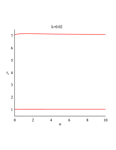
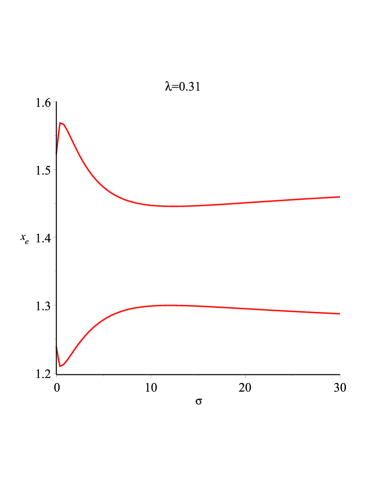
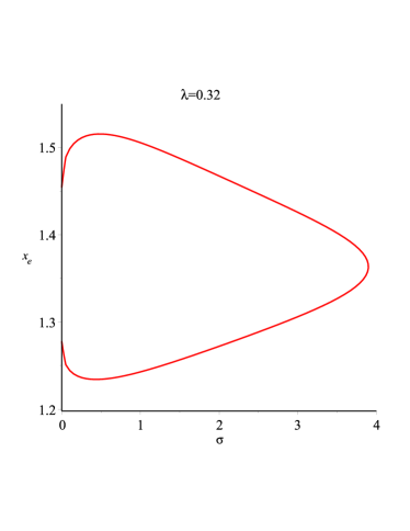
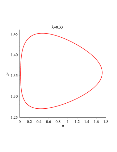
Figure 1: Diagrams of the black hole event horizons $x_{e}$ versus observer acceleration parameter $\sigma$ for dimensionless cosmological parameter $0.2<\lambda<0.33.$ There are not obtained other diagrams for $\lambda<0.2$ and $\lambda>0.33$

We plot all possible solutions of the above horizon equation versus the $\sigma$ parameter of the accelerating observer in figures 1 and 2 for positive and negative numeric values of the dimensionless cosmological parameter respectively in which

$$x_{e}=\frac{r_{e}}{2M},~{}~{}~{}~{}~{}\lambda=\frac{4M^{2}\Lambda}{3}.$$ (38)

These diagrams show that relative distance of two horizons of this black hole is depended to numeric value of vector field or acceleration parameter of preferred reference frame and this distance is decreased by increasing the acceleration parameter. In fact there is particular numeric value for this parameter in which both of black hole horizon and cosmological horizon reach to each other. After some talk about the initial constants and by redefining them with the physical parameters for $\beta(r)$ we set $C_{1,2}=0$ and then we substitute (32) into (24) to obtain $\alpha(r)$ such that

$$2\epsilon\alpha(r)=-4\epsilon\beta(r)=-2\bigg{(}\frac{2M}{r}\bigg{)}^{s_{0}-1}-\frac{2\Lambda r^{2}}{3}+2\mu\ln\bigg{(}\frac{r}{2M}\bigg{)}$$ (39)

and so $\alpha(r)$ term in the equation (9) become

$$e^{2\epsilon\alpha(r)}\approx 1+2\epsilon\alpha(r)=1-2\bigg{(}\frac{2M}{r}\bigg{)}^{s_{0}-1}-\frac{2\Lambda}{3}r^{2}+2\mu\ln\bigg{(}\frac{r}{2M}\bigg{)}.$$ (40)

Substituting (30) and (39) and condition

$$a+\epsilon p=0$$ (41)

into the equation (15) we obtain

$$r^{2}\psi^{\prime\prime}+2r\psi^{\prime}+4\psi=$$ (42)

$$\frac{\gamma_{1}\Lambda r^{2}}{3\epsilon}+\frac{\gamma_{2}}{2\epsilon}\bigg{(}\frac{2M}{r}\bigg{)}^{s_{0}-1}-\frac{3\mu}{\epsilon}\ln\bigg{(}\frac{r}{2M}\bigg{)}+\frac{\gamma_{3}\mu}{2\epsilon}-\frac{2(1+2\sigma)}{\epsilon}+8\sigma.$$

The condition (41) is important because it makes possible an analytic solution for the above differential equation as follows.

$$\psi(r)=\sqrt{\frac{2M}{r}}\bigg{\{}C_{5}\sin\bigg{(}\frac{\sqrt{15}}{2}\ln\bigg{(}\frac{r}{2M}\bigg{)}\bigg{)}+C_{6}\cos\bigg{(}\frac{\sqrt{15}}{2}\ln\bigg{(}\frac{r}{2M}\bigg{)}\bigg{)}\bigg{\}}$$ (43)

$$-\frac{3\mu}{4\epsilon}\ln\bigg{(}\frac{r}{2M}\bigg{)}+\frac{\gamma_{1}\Lambda r^{2}}{30\epsilon}+\frac{\gamma_{2}}{2\epsilon(s_{0}^{2}-3s_{0}+6)}\bigg{(}\frac{2M}{r}\bigg{)}^{s_{0}-1}$$

$$+\frac{\mu(3+2\gamma_{3})+16\sigma(2\epsilon-1)-8}{16\epsilon}$$

where $C_{5,6}$ are integral constants and

$$\gamma_{1}=2A_{1}+2A_{3}+3-A_{2}-A_{4}$$ (44)

$$\gamma_{2}=6+(s_{0}-1)[A_{4}-2A_{3}+s_{0}(2A_{1}-A_{2})]$$ (45)

$$\gamma_{3}=2A_{1}-A_{2}-2A_{3}+A_{4}.$$ (46)

Looking at the definition of the Brans Dicke field (8) and series expansion (9) and substituting the $\psi$ solution (43) we obtain

$$G\phi(r)\approx\frac{1}{2}+\sigma(2\epsilon-1)+\frac{\mu(3+2\gamma_{3})}{16}-\frac{3\mu}{4}\ln\bigg{(}\frac{r}{2M}\bigg{)}$$ (47)

$$+\frac{\gamma_{2}}{2(s_{0}^{2}-3s_{0}+6)}\bigg{(}\frac{2M}{r}\bigg{)}^{s_{0}-1}+\frac{\gamma_{1}\Lambda r^{2}}{30}+$$

$$\sqrt{\frac{2M}{r}}\bigg{\{}\epsilon C_{5}\sin\bigg{(}\frac{\sqrt{15}}{2}\ln\bigg{(}\frac{r}{2M}\bigg{)}\bigg{)}+\epsilon C_{6}\cos\bigg{(}\frac{\sqrt{15}}{2}\ln\bigg{(}\frac{r}{2M}\bigg{)}\bigg{)}\bigg{\}}.$$

Physically we know that $\phi(r)$ should be positive raising function versus $r$ because inverse of the Brans Dicke scalar field is the Newton‘s gravity coupling parameter and in according to the Mach‘s principle $G(r)=Ge^{-\epsilon\psi(r)}$ should be decreasing function [25]. In this sense for $\Lambda>0$ we should choose $\gamma_{1}>0.$ Substituting the coefficients (17), (18), (19) and (20) into (44) we obtain

$$\gamma_{1}=27+18\sigma+\epsilon\{(16\sqrt{1+\sigma}-192)\sigma^{2}-4\sqrt{1+\sigma}(3+4\sqrt{\sigma})\sigma^{\frac{3}{2}}$$ (48)

$$+(16\sqrt{1+\sigma}-32\sqrt{\sigma(1+\sigma)}-612)\sigma+\sqrt{\sigma(1+\sigma)}(64+64\sigma-16\sqrt{\sigma})$$

$$-420+32\sqrt{\sigma(1+\sigma)}$$

and

$$\mu(\sigma)=\frac{2\epsilon\sigma}{(1+\sigma)(1-\delta)[1-4\epsilon(9+4\sigma-\sqrt{\sigma(1+\sigma)(2-\sqrt{\sigma})})]}.$$ (49)

One can check for $\gamma_{1}>0$ and $\sigma>0$ the equation (48) reads to condition $\epsilon<\frac{1}{15}.$ Thus we will use ansatz

$$\epsilon=\frac{1}{50}$$ (50)

in what follows. Regarding (50) we plot diagrams for $\gamma_{1},\delta,\mu$ and $\omega$ versus $\sigma>0$ in figure 3. They show different possible metric solutions in presence of the vector field effects. They show convergent mass function for $\delta<0$ and divergent mass function for $\delta>0.$ However diagram in figure 3-a shows to have $\gamma_{1}>0$ we must be choose $0<\sigma<6.$ Regarding these boundary conditions on the parameters of the metric solution we investigate gravitational lensing of this obtained black hole metric via approaches of wave optics and geometric optics in the next section.

3 Theory of Fresnel-Kirchhoff diffraction

We should remember that the Fresnel Kirchhoff diffraction is applicable when source is far from the observer and so fringe of light waves are formed on the telescope eyepiece .Hence this diffraction will be applicable in study image formation from gravitational lensing in which the stars (sources) and the black holes (the lens) are far from us. The first we review the general formalism of gravitational lensing via wave optics approximation. Ignoring the polarization property the electromagnetic waves can considered just as scalar waves which propagate on a curved space time. For simplicity we choose here a massless scalar wave which is defined by the following equation.

$$\partial_{\mu}(\sqrt{-g}g^{\mu\nu}\partial_{\nu}\Phi)=0$$ (51)

in which $g_{\mu\nu}$ is background metric field which has role of a gravitational lens and $g$ is absolute value of determinant of it. In weak gravitational field limits we consider the background metric of a static object (the lens) has the following form in units $c=G=1$.

$$ds^{2}\approx-(1+2U(\tilde{r}))dt^{2}+(1-2U(\tilde{r}))(d\tilde{r}^{2}+\tilde{r}^{2}(d\theta^{2}+\sin^{2}\theta d\varphi^{2}))$$ (52)

where $|U(\tilde{r})|<<1$ and for our model is given by (32) as follows.

$$2U(\tilde{r})=-\bigg{(}\frac{2M}{\tilde{r}}\bigg{)}^{1+\delta}-\frac{\Lambda\tilde{r}^{2}}{3}+\mu\ln\bigg{(}\frac{\tilde{r}}{2M}\bigg{)}$$ (53)

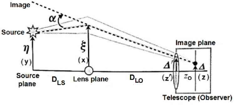
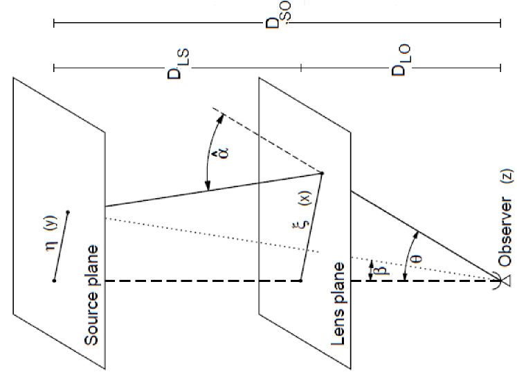
Figure 4: Geometry of the gravitational lens (a) from [16] and (b) from [28] respectively with some minor revisions

in which $\tilde{r}$ is the radial coordinate evaluated from center of the black hole (the lens plane in figure 4). The line element (52) is in fact the Minkowskian flat metric plus small disturbance due to the gravitational potential $U(\tilde{r}).$ To study diffraction of light of a star located at the source plane (see figure 4) via the black hole we must first use a local spherical coordinates system which its center is in the source position and its polar axis is pointing toward the lens (black hole) and then we act to solve wave equation (51). In this sense $U(\tilde{r})$ should be changed by $U(|\vec{r}-\vec{D}_{LS}|)=U(r,\overrightarrow{\theta})$ in which $\vec{D}_{LS}$ is vector distance between source and lens in figure 4, $\overrightarrow{\theta}=\theta(\cos\varphi,\sin\varphi)$ is a two dimensional vector on a flat lens plane and radial coordinate $r$ should be evaluated from the source position instead of the lens position (see figure 4) so that

$$\tilde{r}=|\overrightarrow{r}-\overrightarrow{D}_{LS}|=\sqrt{r^{2}-2rD_{LS}\cos\theta+D_{LS}^{2}}.$$ (54)

Substituting

$$\phi(t,\vec{r})=\tilde{\phi}(\vec{r})e^{-i\varpi t}$$ (55)

into the wave equation (51) and eliminating higher order terms in $U$ one can obtain equation of the amplitude $\tilde{\phi}(\vec{r})$ as

$$(\nabla^{2}+\varpi^{2})\tilde{\phi}=4\varpi^{2}U(\vec{r})\tilde{\phi}$$ (56)

where $\nabla^{2}$ is the flat space Laplacian. By using the spherical polar coordinates system the amplitude equation (56) reads

$$\frac{1}{r}\frac{\partial^{2}}{\partial r^{2}}(r\tilde{\phi})+\frac{1}{r^{2}\sin\theta}\frac{\partial}{\partial\theta}\bigg{(}\sin\theta\frac{\partial\tilde{\phi}}{\partial\theta}\bigg{)}+\frac{1}{r^{2}\sin^{2}\theta}\frac{\partial^{2}\tilde{\phi}}{\partial\varphi^{2}}+\varpi^{2}\tilde{\phi}(\vec{r})=4\varpi^{2}U(\vec{r})\tilde{\phi}(\vec{r}).$$ (57)

We assume the wave scattering occurs in a small spatial region around the lens and outside of this region the wave propagates in a flat space. In other words one can see that without the lensing object for which $U=0$ the above equation has a simple solution as

$$\tilde{\phi}_{0}=\frac{\Omega e^{i\varpi r}}{r}$$ (58)

in which $\Omega$ is a constant and $r=|\vec{r}|$. Hence it is useful we act to define the amplification factor of the wave amplitude due to lensing as follows.

$$F(\vec{r})=\frac{\tilde{\phi}(\vec{r})}{\tilde{\phi}_{0}(\vec{r})}.$$ (59)

We set the observer is located at $\vec{r}_{o}=(r_{o},\theta_{o},\varphi_{o})$ with $\theta_{o}<<1(radians)$ on the observer plane (see figure 4). In this case the waves which is detected by the observer should be confined in the small $\theta<<1$ regions with $0\leq\varphi\leq 2\pi$ for which the approximation $\sin\theta\approx\theta$ can be used in the equation (57) . Substituting (58) and (59) and the approximation $\sin\theta\approx\theta,$ the equation (57) reduces to the following form.

$$\frac{\partial^{2}F}{\partial r^{2}}+2i\varpi\frac{\partial F}{\partial r}+\frac{\nabla^{2}_{\theta}F}{r^{2}}=4\varpi^{2}U(r,\theta)F$$ (60)

where we defined

$$\nabla^{2}_{\theta}=\frac{\partial^{2}}{\partial\theta^{2}}+\frac{1}{\theta}\frac{\partial}{\partial\theta}+\frac{1}{\theta^{2}}\frac{\partial^{2}}{\partial\varphi^{2}}.$$ (61)

According to the work presented in Refs. [15, 16] we choose geometry of the gravitational lens to be made by three parallel planes, namely the source plane, the lens plane and the observer plane (see figure 4). The angular diameter distances along the normal from the observer plane to the source and the lens planes are labeled with $D_{SO}$ and $D_{LO}$, respectively. Distance between the source and the lens planes is labeled as $D_{LS}.$ The emitted waves by a point source located in the source plane, travel freely to the lens plane, and they are lensed by a gravitational potential $U$ where they are assumed to be localized in the thin (width$<<$ focal length) lens plane , before reaching the telescope at the observer plane. We assume $\overrightarrow{\xi}$ is the coordinates at the lens plane, $\overrightarrow{\eta}$ is the coordinates at the source plane and $\vec{\Delta}$ is coordinates at the observer plane in figure 4, which can be redefined by the following dimensionless coordinates respectively.

$$\overrightarrow{x}=\frac{\overrightarrow{\xi}}{\xi_{0}}=\frac{\vec{\theta}}{\theta_{E}},~{}~{}~{}\overrightarrow{y}=\frac{D_{LO}}{D_{SO}}\frac{\overrightarrow{\eta}}{\xi_{0}}=\frac{\vec{\beta}}{\theta_{E}},~{}~{}~{}~{}~{}\vec{z}=\bigg{(}1-\frac{D_{LO}}{D_{SO}}\bigg{)}\frac{\vec{\Delta}}{\xi_{0}}$$ (62)

where $\xi_{0}=D_{LO}\theta_{E}$ is radius of the Einstein rings and $\theta_{E}$ is corresponding angular radius which for a point lens with mass $M_{L}$ is given by the following equation.

$$\theta_{E}=2\sqrt{\frac{M_{L}}{D_{LO}}\frac{D_{LS}}{D_{SO}}}.$$ (63)

Applying (62) and (63) one can show that the equation (60) has an integral solution (see [16] and [5]) which at the observer plane is given by

$$F(\vec{y},\vec{z})=\frac{w}{2\pi i}\int dx^{2}e^{iwT(x,y,z)}.$$ (64)

This integral solution is called as Fresnel-Kirchhoff diffraction formula. The dimensionless time delay function $T(x,y,z)$ and dimensionless frequency $w$ are given respectively by the following relations.

$$T(x,y,z)=\frac{1}{2}|\overrightarrow{x}-\overrightarrow{y}-\vec{z}|^{2}-\Psi(\overrightarrow{x}),~{}~{}~{}~{}w=\frac{D_{SO}\xi_{0}^{2}}{D_{{LS}}D_{LO}}\varpi=4M_{L}\varpi$$ (65)

in which 2 dimensional lens potential is defined by the following equation.

$$\Psi(\overrightarrow{x})=\frac{1}{2M_{L}}\int_{\ell}^{D_{SO}}drU(\overrightarrow{x},r)$$ (66)

where $\ell$ is scale of source. In fact it is obtained by projecting the three dimensional metric potential $U(r,\vec{\theta})$ on the lens plane. This lens potential satisfies two important properties as follows: According the following equation its gradient become deflection angle.

$$\overrightarrow{\nabla_{x}}\Psi(\overrightarrow{x})=\overrightarrow{\alpha}(\overrightarrow{x})$$ (67)

and its two dimensional Laplacian gives twice of the convergence as

$$\nabla^{2}_{x}\Psi(\overrightarrow{x})=2\kappa(\overrightarrow{x})$$ (68)

where

$$\kappa(\overrightarrow{x})=\frac{\Sigma(\overrightarrow{x})}{\Sigma_{cr}}$$ (69)

is in fact the dimensionless surface gravity $\Sigma(\overrightarrow{x})$ of the lens evaluated on the lens plane and

$$\Sigma_{cr}=\frac{D_{SO}}{4\pi D_{LO}D_{LS}}$$ (70)

is called the critical surface gravity. The time delay $T(x,y,z)$ can be obtained by applying the path integral formalism on the possible pathes of the moving light rays by regarding the eikonal approximation in the equation (60). In the eikonal approximation one can neglect second order differentiation with the first one in the equation (60) because of the assumption $\varpi/|\partial\ln F/\partial r|\sim$(Scale on which $F$ varies)/(wavelength)$>>1$ and so the equation (60) looks like the Schrodinger equation [5]. In this latter case the $r$ component behaves same as the time evolution parameter for the wavefronts with particle mass $\varpi$. In the geometrical optics limit $\varpi>>1$ the diffraction integral (64) reaches to the stationary points of the phase function which they are obtained by the Fermat‘s principle as follows.

$$\overrightarrow{\nabla_{x}}T(x,y,z)=0=\overrightarrow{x}-\overrightarrow{y}-\vec{z}-\overrightarrow{\alpha}(\overrightarrow{x})$$ (71)

in which the source position $\overrightarrow{y}$ is fixed. This is lens equation in geometrical approximation for gravitational lensing and determines the location of the images $\overrightarrow{x}$ for a given source position $\overrightarrow{y}.$ At the observer plane the unlensed wave amplitude (58) is $\phi_{o}(\vec{\eta},\vec{\Delta})=(\Omega/r_{s})\exp(i\varpi r_{s})$ where $r_{s}=\sqrt{D_{SO}^{2}+|\vec{\eta}-\vec{\Delta}|^{2}}.$ At the Fresnel-Kirchhoff diffraction limit for which $D_{SO}>>|\vec{\eta}-\vec{\Delta}|$ we can write $\phi_{o}(\vec{\eta},\vec{\Delta})\approx(\Omega/D_{SO})\exp[i\varpi(D_{SO}+|\vec{\eta}-\vec{\Delta}|^{2}/2D_{SO})]$ and then we substitute the dimensionless coordinates (62) to obtain [15, 16]

$$\phi_{0}(\vec{y},\vec{z})=\frac{\Omega e^{iwt(\vec{y},\vec{z})}}{D_{SO}}.$$ (72)

In the above relation

$$t(\vec{y},\vec{z})=\frac{1}{2}\sqrt{\frac{p}{1-p}}\bigg{|}\sqrt{\frac{p}{1-p}}\vec{y}-\sqrt{\frac{1-p}{p}}\vec{z}\bigg{|}^{2}+\bigg{(}\frac{1-p}{2q}\bigg{)}$$ (73)

and

$$p=\frac{D_{LS}}{D_{SO}},~{}~{}~{}q=\frac{2M_{L}}{D_{SO}},~{}~{}~{}$$ (74)

and so the lensed wave amplitude will be

$$\phi_{L}(\vec{y},\vec{z})=\phi_{0}(\vec{y},\vec{z})F(\vec{y},\vec{z}).$$ (75)

This is an entrance wave which enters in front of the telescope convex lens (see figure 4-a) and so part of it which passes through the lens makes the transmitted wave at the observer plane (the telescope) which is given by the following equation.

$$\phi_{T}(\vec{y},\vec{z^{\prime}})=\tau(\vec{z^{\prime}})e^{-i\varepsilon w|\vec{z^{\prime}}|^{2}}\phi_{L}(\vec{y},\vec{z^{\prime}}),~{}~{}~{}\varepsilon=\frac{D_{LO}D_{SO}}{2fD_{LS}}.$$ (76)

Here $z^{\prime}$ and $f$ are position and focal length of the telescope convex lens respectively. The function of aperture of the convex lens $\tau(\vec{z^{\prime}})$ is defined by $\tau(\vec{z})=1$ for $0\leq|\vec{z}|\leq R$ and $\tau(\vec{z})=0$ for $|\vec{z}|>R$ in which $R$ is lens radius of the telescope. We apply the lens equation of a convex thin lens as

$$\frac{1}{D_{SO}}+\frac{1}{z_{o}}=\frac{1}{f}$$ (77)

to obtain amplitude of the magnified wave which after passing from the lens causes to form the image at the position $zo$ on the observer plane. This is done by the integral equation

$$\phi_{o}(\vec{y},\vec{z})=\int_{|\vec{z^{\prime}}|\leq R}dz^{\prime 2}\phi_{T}(\vec{y},\vec{z^{\prime}})e^{i(\varepsilon wf/z_{o})|\vec{z}-\vec{z^{\prime}}|^{2}}.$$ (78)

By substituting (72), (75) and (76) into the equation (78) we obtain

$$\phi_{o}(\vec{y},\vec{z})=\frac{\Omega\exp[iwg(\vec{y},\vec{z})]}{D_{SO}}\int_{|\vec{z^{\prime}}|\leq R}dz^{\prime 2}F(\vec{y},\vec{z^{\prime}})e^{-iw\vec{k}\cdot\vec{z^{\prime}}}$$ (79)

where

$$g(\vec{y},\vec{z})=\bigg{(}\frac{p}{1-p}\bigg{)}^{\frac{3}{2}}\frac{y^{2}}{2}+\frac{D_{LO}}{2pz_{o}}z^{2}+\frac{1-p}{2q}$$ (80)

and

$$\vec{k}=\sqrt{\frac{p}{1-p}}\vec{y}+\frac{D_{LO}}{pz_{o}}\vec{z}$$ (81)

and in the exponent we omitted $|\vec{z^{\prime}}|^{2}$ with respect to the linear orders . Because evaluate of the integral is in a small region $|z^{\prime}|\leq R$ in which dimensionless radius of the telescope convex lens is small $R<<1.$ In fact $R$ is the convex lens radius divided by $D_{SO}.$ On the other side we know that distance between the source and the observer is very large versus radius of the convex lens in the Fraunhofer diffraction. However one can look at the equation (79) to infer that $\phi_{o}(\vec{y},\vec{z})$ is in fact the Fourier transform of the amplification factor $F$ which produces the interference fringe pattern. Furthermore the lens equation (77) shows that for large distances $D_{SO}>>1$ we will have

$$z_{o}\approx f.$$ (82)

By substituting the above approximation into (80) and (81) and by applying (65) and (64), the equation (79) reaches to the following form.

$$\phi_{o}(\vec{y},\vec{z})\approx\frac{\Omega w\exp[iwg(\vec{y},\vec{z})]}{2\pi iD_{SO}}\int dx^{2}\exp[iw(|\vec{x}-\vec{y}|^{2}/2-\psi(\vec{x}))]\times$$ (83)

$$\int_{0}^{R}z^{\prime}dz^{\prime}\int_{0}^{2\pi}d\chi\exp(-iw\rho z^{\prime}\cos\chi)$$

where $\chi$ is angle between $\vec{\rho}$ and $\vec{z}^{\prime}$ and

$$\vec{\rho}=\vec{x}+\bigg{(}\sqrt{\frac{p}{1-p}}-1\bigg{)}\vec{y}+\frac{D_{LO}}{pf}\vec{z}$$ (84)

and we omitted again $z^{\prime 2}$ with respect to its first order term because of above mentioned reasons. By applying integral form of the zero order Bessel function [27]

$$J_{0}(s)=\frac{1}{2\pi}\int_{0}^{2\pi}d\chi e^{-is\cos\chi}$$ (85)

one can calculate the angular $\chi$ part in the integral equation (83) and obtain the zero order Bessel function $J_{0}(w\rho z^{\prime})$ and then by using the identity

$$sJ_{0}(s)=\frac{d(sJ_{1}(s))}{ds}$$ (86)

at last the equation (83) reaches to the following form.

$$\phi_{o}(\vec{y},\vec{z})=\frac{\Omega R\exp[iwg(y,z)]}{iD_{SO}}\int dx^{2}\frac{J_{1}(wR\rho)}{\rho}e^{iw(|\vec{x}-\vec{y}|^{2}/2-\Psi(x))}.$$ (87)

At the geometrical optics limit where $w>>1$ the amplification factor (64) approaches to the WKB approximated form as

$$F(x_{s},z)\sim\frac{w}{2\pi i}e^{iw(|\vec{x}_{s}-\vec{y}-\vec{z}|^{2}/2-\psi(\vec{x_{s}}))}$$ (88)

where positions of the stationary images $\vec{x}_{s}$ are obtained from the lens equation (71) and so the image amplification factor (87) reduces to the following form.

$$\phi_{o}(\vec{z},\vec{x}_{s})\sim\exp\{i\frac{w}{2}[2g(\vec{y},\vec{z})+|\vec{x}_{s}-\vec{y}-\vec{z}|^{2}-2\psi(\vec{x_{s}})]\}\frac{J_{1}(wR\rho_{s})}{wR\rho_{s}}$$ (89)

in which we should use (71) to obtain images position $x_{s}$ versus the fixed source position $y$ and replace into the above equation. Also the above Bessel function reduces to a two-dimensional Dirac delta function in geometric optics limit $wR>>1$ such that we can use

$$\lim_{wR\to\infty}\phi_{o}(\vec{y},\vec{z})\sim\delta^{2}(wR\rho_{s}).$$ (90)

This amplitude of the wave gives us position of the images at the observer plane in the geometrical optics limit $\rho_{s}=0$ which can be rewritten as follows.

$$\vec{z}_{s}=\frac{pf}{D_{LO}}\bigg{[}\bigg{(}1-\sqrt{\frac{p}{1-p}}\bigg{)}\vec{y}-\vec{x}_{s}\bigg{]}.$$ (91)

If the lens equation (71) has multiple stationary image positions $\vec{x}_{s}^{i}$ with $i=1,2,...$ then the amplified waves on the observer plane for these stationary images reaches [16] to the following form.

$$\phi_{o}(\vec{z})=\sum_{i=1}\Upsilon_{i}\phi_{o}(\vec{z},\vec{x}_{s}^{i})$$ (92)

where amplitude $\Upsilon_{i}$ should be set as magnitude of image magnification factor in the geometric optics limit as follows.

$$\Upsilon_{i}=\big{(}\frac{y}{x}\frac{dy}{dx}\big{)}^{-1}_{|_{x=x_{s}^{i}}}.$$ (93)

In the next section we use metric potential of our model (5) to calculate corresponding lens potential and then to produce the images via approaches of geometric optics and wave optics.

4 Lens potential

By substituting (54) and (53) into the integral equation of the lens potential (66) we obtain

$$\Psi(\theta)=-\frac{1}{2q}\int_{0}^{1}dx\{\bigg{(}\frac{q}{\sqrt{x^{2}-2xp\cos\theta+p^{2}}}\bigg{)}^{1+\delta}+$$ (94)

$$h(x^{2}-2xp\cos\theta+p^{2})-\mu\ln(\sqrt{x^{2}-2xp\cos\theta+p^{2}}/q)\}$$

where we used (74) and the following definitions

$$~{}~{}~{}~{}h=\frac{\Lambda D_{SO}^{2}}{3},~{}~{}~{}x=\frac{r}{D_{SO}}$$ (95)

and assumed $\ell=0$ because of small scale of the cosmic source from point of view of earth observer. However one can check that the above integral has an analytic solution just for integer numeric values for $\delta$ parameter and before to calculate it we must be substitute numeric value for $\delta.$ All possible numeric values for $\delta$ parameter are given in figure (3-b) . We will need asymptotic behavior of the lens potential at $\sin\theta\approx\theta$ which we used previously in the Laplacian (60). In this sense one can check that the lens potential is singular namely at limits $\theta\to 0$ it diverges to infinity just for $\delta>0$ but not for $\delta<0.$ First term in Taylor series of lens potential of our model begins by $\frac{1}{\theta^{\delta}}$ in which $\delta>0.$ We also claim that $\delta<0$ gives not physical metric solutions because the function of black hole mass (34) should be an increasing function by raising $r.$ In these sense we calculate Taylor series expansion of the integral equation (94) for ansatz $\delta=0,1,2,3$ respectively as follows.

$$\Psi^{\delta=0}(\theta)=\Psi_{0}^{0}+\ln\theta+\Psi_{1}^{0}\theta+O(\theta^{2})$$ (96)

where

$$\Psi_{0}^{0}=-\frac{1}{2q}\bigg{[}\mu+\frac{h}{12}+\frac{(1-\mu)\pi i}{4}+\ln(q2^{1+2q})\bigg{]},~{}~{}~{}\Psi_{1}^{0}=\frac{\mu\pi}{4q}$$ (97)

$$\Psi^{\delta=1}(\theta)\approx\frac{\Psi^{1}_{-1}}{\theta}+\Psi^{1}_{0}+\Psi^{1}_{1}\theta+O(\theta^{2})$$ (98)

where

$$\Psi^{1}_{-1}=-\frac{\pi q}{2p},~{}~{}~{}\Psi^{1}_{1}=\frac{\pi(6\mu p-q^{2})}{12q}$$ (99)

and

$$\Psi^{1}_{0}=\frac{1}{2q}\bigg{\{}\frac{q^{2}(p-2)}{p(p-1)}-\frac{h}{3}+hp-hp^{2}+\mu\ln\bigg{(}\frac{p^{p}}{(1-p)^{p-1/2}}\bigg{)}\bigg{\}}.$$ (100)

$$\Psi^{\delta=2}(\theta)=\frac{\Psi_{-2}^{2}}{\theta^{2}}+\Psi^{2}_{0}+\Psi^{2}_{1}\theta+O(\theta^{2})$$ (101)

where

$$\Psi_{-2}^{2}=-\frac{q^{2}(1+p)}{2p^{2}},~{}~{}~{}\Psi_{1}^{2}=\frac{\mu\pi p}{2q}$$ (102)

and

$$\Psi_{0}^{2}=\frac{1}{2q}\bigg{\{}\frac{q^{3}}{2(1-p)^{2}}-\frac{q^{3}(2+p)}{64p^{2}(1-p)}-\frac{h}{3}+hp-hp^{2}-\mu+$$ (103)

$$\mu\ln\bigg{(}\frac{p^{p}(1-p)^{1-p}}{q}\bigg{)}+\frac{q^{2}}{12p^{2}}\bigg{\}}.$$

$$\Psi^{\delta=3}(\theta)=\frac{\Psi^{3}_{-3}}{\theta^{3}}+\frac{\Psi_{-2}^{3}}{\theta^{2}}+\frac{\Psi_{-1}^{3}}{\theta}+\Psi_{0}^{3}+\Psi_{1}^{3}\theta+O(\theta^{2})$$ (104)

where we defined

$$\Psi_{-3}^{3}=-\frac{\pi q^{3}}{4p^{3}},~{}~{}~{}\Psi_{-2}^{2}=-\frac{q^{3}(1-2p)}{4p^{3}(1-p)^{2}},~{}~{}~{}\Psi_{-1}^{3}=-\frac{\Psi_{-3}^{3}}{2}$$ (105)

and

$$\Psi_{0}^{3}=\frac{1}{2q}\bigg{\{}\frac{q^{4}}{3p^{3}}+\frac{q^{4}}{3(1-p)^{3}}-\frac{h}{3}+hp-hp^{2}-\mu+\mu\ln\bigg{(}\frac{p^{p}(1-p)^{1-p}}{q}\bigg{)}\bigg{\}}$$ (106)

$$\Psi_{1}^{3}=\frac{\pi(240\mu p^{4}-17q^{4})}{480qp^{3}}.$$ (107)

By looking at the above lens potentials we infer that $\delta=0$ with logarithmic singularity at $\theta\to 0$ corresponds to a point lens while $\delta=1,2,3,\cdots$ correspond with non point lens which their spatial distributions of mass are given by (34). Looking at these lens potentials one can infer that the vector field effects with $\mu(\sigma)\neq 0$ (see eq. (49)) remove logarithmic singularity but creates a power law singularity $\theta^{-\delta}$ for $\delta>0$ for the lens potential. It is obvious this will affect the position of the images. We are now in position to calculate images magnification factor (64) for the above lens potentials as follows.

4.1 Images magnification factor

To calculate the magnification factor (64) of the lensed waves, we choose a two dimensional polar coordinates on the lens plane for which the surface differential is $dx^{2}=xdxd\zeta$ where $\zeta$ is polar angle between directions of the vectors $\vec{x}$ and $\vec{y}+\vec{z}$ on the lens plane so that $|\vec{x}-(\vec{y}+\vec{z})|^{2}=x^{2}+|\vec{y}+\vec{z}|^{2}-2x|\vec{y}+\vec{z}|\cos\zeta.$ Applying these relations the equation (64) can be rewritten as follow.

$$F(y,z)=-iwe^{(iw/2)|\vec{y}+\vec{z}|^{2}}\int_{0}^{\infty}xdxJ_{0}(wx|\vec{y}+\vec{z}|)e^{iw[\frac{x^{2}}{2}-\Psi(x)]}$$ (108)

in which we substituted the following identity for the zero order Bessel function.

$$J_{0}(wx|\vec{y}+\vec{z}|)=\frac{1}{2\pi}\int_{0}^{2\pi}d\zeta e^{-iwx|\vec{y}+\vec{z}|\cos\zeta}.$$ (109)

Substituting the series solution [27]

$$J_{0}(s)=\sum_{k=0}^{\infty}\frac{(-1)^{k}}{(k!)^{2}}\bigg{(}\frac{s}{2}\bigg{)}^{2k}$$ (110)

the integral equation (108) reads

$$F(y,z)=-iwe^{(iw/2)|\vec{y}+\vec{z}|^{2}}\sum_{k=0}^{\infty}\frac{(-1)^{k}}{(k!)^{2}}C_{k}\bigg{(}\frac{w|\vec{y}+\vec{z}|}{2}\bigg{)}^{2k}$$ (111)

where we defined

$$C_{k}=\int_{0}^{\infty}x^{1+2k}e^{iw[x^{2}/2-\Psi(x)]}dx.$$ (112)

We see that numeric values of the coefficients $C_{k}$ are dependent to form of the lens potential. By substituting $\theta=\theta_{E}x$ into the lens potentials (96), (98) and (101) and (104) and by keeping just highest order singular term in these potentials to calculate (112) and by using the integral form of the gamma function $n!=\int_{0}^{\infty}t^{n}e^{-t}dt$ [27] at last we obtain

$$C^{\delta=0}_{k}\approx e^{-iw(\Psi^{0}_{0}+2\ln\theta_{E})}2^{1+k-iw/2}\bigg{(}\frac{i}{w}\bigg{)}^{1+k-iw/2}\bigg{(}k-\frac{iw}{2}\bigg{)}!$$ (113)

for point source $\delta=0$ and for non point sources $\delta=1,2,3$ we have

$$C_{k}^{\delta}\approx e^{-iw\Psi^{\delta}_{0}}\int_{0}^{\infty}dxx^{1+2k}e^{iw\Pi(x)}$$ (114)

where

$$\Pi(x)=\frac{x^{2}}{2}-\frac{\Psi_{-\delta}^{\delta}}{\theta_{E}^{\delta}}\frac{1}{x^{\delta}}$$ (115)

has Taylor series expansion around its minimum point

$$x_{m}=\bigg{(}\frac{-\delta\Psi_{-\delta}^{\delta}}{\theta_{E}^{\delta}}\bigg{)}^{\frac{1}{2+\delta}},~{}~{}~{}\theta_{E}=\sqrt{\frac{2pq}{1-p}}$$ (116)

as follows.

$$\Pi(x)\approx\bigg{(}\frac{2+\delta}{2\delta}\bigg{)}x_{m}^{2}+\frac{(1+\delta)}{2}(x-x_{m})^{2}+O(3).$$ (117)

Substituting (117) into (114) one can show

$$C^{\delta}_{k}\approx e^{iw[(2+\delta)x_{m}^{2}/2\delta-\Psi_{0}^{\delta}]}\int_{0}^{\infty}dxx^{1+2k}e^{iw(1+\delta)(x-x_{m})^{2}/2}.$$ (118)

Because $|x_{m}|<1$ then we can use Taylor series of the above integral equation around $x_{m}$ and substitute integral form of the gamma function to obtain a series form of the solution for the coefficients (118). This is done as follows.

$$C^{\delta}_{k}\approx e^{iw[(2+\delta)x_{m}^{2}/2\delta-\Psi_{0}^{\delta}]}\bigg{(}\frac{i}{w(1+\delta)}\bigg{)}^{1+k}2^{k}k!\times$$ (119)

$$\bigg{\{}1+x_{m}\frac{(k+\frac{1}{2})!}{k!}\bigg{(}\frac{2w(1+\delta)}{i}\bigg{)}^{\frac{1}{2}}+x_{m}^{2}[1-iw(1+\delta)(1+k)]+O(x_{m}^{3})\bigg{\}}.$$

By substituting (113) into the image magnification factor (111) we will have

$$F_{\delta=0}(y,z)=2e^{-iw[2\ln\theta_{E}+\Psi_{0}^{0}-|\vec{y}+\vec{z}|^{2}/2]}\bigg{(}\frac{2i}{w}\bigg{)}^{-iw/2}\times$$ (120)

$$\sum_{k=0}^{\infty}\frac{(k-iw/2)!}{(k!)^{2}}\bigg{(}\frac{-iw|\vec{y}+\vec{z}|^{2}}{2}\bigg{)}^{k}.$$

In usual astrophysical situations we know that [5]

$$w=4M_{L}\omega\sim 10^{5}\times\bigg{(}\frac{M_{L}}{M_{\odot}}\bigg{)}^{\frac{1}{2}}(\nu/GHz)>>1$$ (121)

and so it is useful we study asymptotic behavior of the amplification factor (120) for $w>>1$ as follows. Consider

$$\frac{\big{(}k-\frac{iw}{2}\big{)}!}{\big{(}-\frac{iw}{2}\big{)}!}=\bigg{(}-\frac{iw}{2}\bigg{)}\bigg{(}-\frac{iw}{2}+1\bigg{)}\bigg{(}-\frac{iw}{2}+2\bigg{)}\cdots\bigg{(}-\frac{iw}{2}+k\bigg{)}$$

$$=\bigg{(}-\frac{iw}{2}\bigg{)}^{k}\bigg{(}1+\frac{2}{iw}\bigg{)}\bigg{(}1+\frac{4}{iw}\bigg{)}\cdots\bigg{(}1+\frac{2k}{iw}\bigg{)}$$ (122)

which for large frequency $w>>1$ one can omit the negligible terms so that $\big{(}1+\frac{2}{iw}\big{)}\big{(}1+\frac{4}{iw}\big{)}\cdots\big{(}1+\frac{2k}{iw}\big{)}$ and so we can write

$$\lim_{w\to\infty}\frac{\big{(}k-\frac{iw}{2}\big{)}!}{\big{(}-\frac{iw}{2}\big{)}!}\cong\bigg{(}-\frac{iw}{2}\bigg{)}^{k}.$$ (123)

On the other side for large frequencies $w>>1$ the following identity is satisfied.

$$\lim_{w\to\infty}\bigg{(}\frac{-iw}{2}\bigg{)}!\approx\bigg{(}\frac{-iw}{2}\bigg{)}^{-\frac{iw}{2}}.$$ (124)

By substituting (123) and (124) into the equation (120) we obtain

$$F_{\delta=0}(y,z,w>>1)\approx 2e^{-iw[2\ln\theta_{E}+\Psi_{0}^{0}-|\vec{y}+\vec{z}|^{2}/2]}J_{0}(w|\vec{y}+\vec{z}|)$$ (125)

in which we used series form for the zero order Bessel function namely

$$J_{0}(w|\vec{y}+\vec{z}|)=\sum_{k=0}^{\infty}\frac{(-1)^{k}}{(k!)^{2}}\bigg{(}\frac{w}{2}|\vec{y}+\vec{z}|\bigg{)}^{2k}.$$

By substituting (119) into the image magnification factor (111) and then by integrating as step by step for each order of Taylor series at last we obtain the following solution for $\delta=1,2,3,\cdots$.

$$F_{\delta=1,2,3,\cdots}(y,z)=F^{(0)}(y,z)+x_{m}F^{(1)}(y,z)+x_{m}^{2}F^{(2)}(y,z)+O(x_{m}^{3})$$ (126)

where

$$F^{(0)}(y,z)=\frac{1}{(1+\delta)}\exp\bigg{\{}iw\bigg{[}\frac{\delta|\vec{y}+\vec{z}|^{2}}{2(1+\delta)}+\frac{(2+\delta)}{2\delta}x_{m}^{2}-\Psi_{0}^{\delta}\bigg{]}\bigg{\}}$$ (127)

for which we used the identity $e^{s}=\sum_{n=0}^{\infty}s^{n}/n!,$

$$F^{(1)}(y,z)=\sqrt{\frac{w}{1+\delta}}\times$$ (128)

$$\exp\bigg{\{}-\frac{i\pi}{4}+iw\bigg{[}\frac{1}{2}|\vec{y}+\vec{z}|^{2}+\frac{(2+\delta)}{2\delta}x_{m}^{2}-\Psi_{0}^{\delta}\bigg{]}\bigg{\}}\sum_{k=0}^{\infty}\frac{(k+\frac{1}{2})!}{(k!)^{2}}\bigg{(}\frac{-iw|\vec{y}+\vec{z}|^{2}}{2(1+\delta)}\bigg{)}^{k}$$

and

$$F^{(2)}(y,z)=F^{(0)}(y,z)-$$ (129)

$$iw\exp\bigg{\{}iw\bigg{[}\frac{1}{2}|\vec{y}+\vec{z}|^{2}+\frac{(2+\delta)}{2\delta}x_{m}^{2}-\Psi_{0}^{\delta}\bigg{]}\bigg{\}}\sum_{k=0}^{\infty}\frac{(k+1)}{k!}\bigg{(}\frac{-iw|\vec{y}+\vec{z}|^{2}}{2(1+\delta)}\bigg{)}^{k}.$$

By applying the approximations

$$\lim_{k\to\infty}\frac{(1+k)}{k!}=\frac{(1+k)!}{(k!)^{2}}\approx\frac{1}{k!},~{}~{}~{}\lim_{k\to\infty}\frac{(k+\frac{1}{2})!}{(k!)^{2}}\approx\frac{1}{k!}$$ (130)

one can show

$$F^{(1)}(y,z)=\sqrt{2w(1+\delta)}\exp\bigg{(}\frac{-i\pi}{4}\bigg{)}F^{(0)},$$ (131)

$$~{}~{}~{}F^{(2)}(y,z)=[1-iw(1+\delta)]F^{(0)}(y,z)$$

and so we can write

$$F_{\delta=1,2,3,\cdots}(y,z)=\frac{\{1+\sqrt{2w(1+\delta)}\exp(-i\pi/4)x_{m}+[1-iw(1+\delta)]x_{m}^{2}\}}{(1+\delta)}\times$$ (132)

$$\exp\bigg{\{}iw\bigg{[}\frac{\delta|\vec{y}+\vec{z}|^{2}}{2(1+\delta)}+\frac{(2+\delta)}{2\delta}x_{m}^{2}-\Psi_{0}^{\delta}\bigg{]}\bigg{\}}$$

where we have

$$x_{m}^{\delta=1}=\bigg{[}\frac{\pi\sqrt{q}}{2p}\bigg{(}\frac{1-p}{2p}\bigg{)}^{\frac{1}{2}}\bigg{]}^{\frac{1}{2}},~{}~{}~{}x_{m}^{\delta=2}=\bigg{(}\frac{q(1-p^{2})}{2p^{3}}\bigg{)}^{\frac{1}{3}}$$ (133)

$$x_{m}^{\delta=3}=\bigg{[}\frac{3\pi q^{\frac{3}{2}}}{4p^{3}}\bigg{(}\frac{1-p}{2p}\bigg{)}^{\frac{3}{2}}\bigg{]}^{\frac{1}{4}},~{}~{}~{}\Psi_{-1}^{1}=-\frac{\pi q}{2p},$$

$$~{}~{}~{}\Psi_{-2}^{2}=-\frac{q^{2}(1+p)}{2p^{2}},~{}~{}~{}\Psi_{-3}^{3}=-\frac{\pi q^{3}}{4p^{3}}.$$

At the astrophysical scales we know that $p<1$ and $q<<1$ and so $x_{m}$ defined by the above relations will be have small numeric values. Hence we use ansatz

$$p=\frac{1}{2},~{}~{}~{}q=\frac{1}{10}$$ (134)

for which

$$x_{m}^{\delta=1}=0.83815,~{}~{}~{}x_{m}^{\delta=2}=0.66939,~{}~{}~{}x_{m}^{\delta=3}=0.67755$$ (135)

to plot intensity of the images amplification factor $|F|=\sqrt{FF^{*}}$ versus the frequency $w$ in figures 5 for (125) and (132) respectively which are given by

$$|F_{\delta=0}|=2|J_{0}(w|\vec{y}+\vec{z}|)|$$ (136)

and

$$|F_{\delta=1,2,3,\cdots}|=\{1+2x_{m}\sqrt{w(1+\delta)}+2x_{m}^{2}(1+w(1+\delta))+$$ (137)

$$2x_{m}^{3}\sqrt{w(1+\delta)}[1+w(1+\delta)]+x_{m}^{4}[1+w^{2}(1+\delta)^{2}]\}^{\frac{1}{2}}/(1+\delta).$$

They show raising of the image amplifications factor by increasing $w$ and $x_{m}$ for non point mass $\delta=1,2,3$ but not for point mass $\delta=0.$ In the subsequent section we investigate how can produce the stationary images via interference of waves and geometric optics approaches?

4.2 Images production via interference of waves

At first step we substitute the lens potentials (96), (98), (101) and (104) into the lens equation (71) and then we obtain images positions in the geometric optics approach. To do so we consider just highest order singular terms in the lens potentials. Also we assume that position vector direction of the source and the images are aligned which means the image and the object are on the same page and source plane, image plane and lens plane are parallel with each others. In this sense the lens equations takes a simpler form such that

$$x-y-z-\frac{1}{x}=0$$ (138)

for $\delta=0$

$$x-y-z-\frac{\pi}{p}\sqrt{\frac{q(1-p)}{2p}}\frac{1}{x^{2}}=0$$ (139)

for $\delta=1$

$$x-y-z-\frac{q(1-p^{2})}{2p^{3}}\frac{1}{x^{3}}=0$$ (140)

for $\delta=2$ and

$$x-y-z-\frac{3\pi}{4p^{3}}\bigg{(}\frac{q(1-p)}{2p}\bigg{)}^{\frac{3}{2}}\frac{1}{x^{4}}=0$$ (141)

for $\delta=3$ and so on. To obtain how many images are formed on the observer plane at its center $z=0$, we plot diagrams of the above lens equations for ansatz (134) in figures 6. Looking at these figures one infer that for $\delta=0,2$ there are two different images at each side of the center of the telescope convex lens but not for $\delta=1,3.$ In the latter case just one image is at say right side while three images at left side. This shows that distribution of images on the observer plane are dependent to shape of the mass function of the lens. In other word if numeric value in $\delta$ parameter become even (odd) number then number of images will be (unequal) equal in both side of center of the convex lens of the telescope. Magnification of the images in the geometric optics limit is defined by $\Upsilon=\big{(}\frac{y}{x}\frac{dy}{dx}\big{)}^{-1}$ which by substituting (138), (139), (140) and (141) we plotted its absolute value in figures 7. They show inequality between magnifications of left side images and right side ones when $\delta=1,3$ and more precisely that for left side images the magnifications are greater than that of ones for right side images. To produce stationary images from interference of fringes pattern given by (92) we should calculate images position $x_{i}$ and corresponding magnifications (93) for a fixed source position $y$ by applying the lens equations (138), (139), (140) and (141). Then we substitute them into the (92). We do these for sample source positions $y=0,3,-3$ and collect them in the table 1.

Table 1. Stationary images position and corresponding magnifications for $\delta=0,1,2,3$ and $p=\frac{1}{2},q=\frac{1}{10}$ at $z=0$

$\delta$	$y$	$(x_{1},|\Upsilon_{1}|)$	$(x_{2},|\Upsilon_{2}|)$	$(x_{3},|\Upsilon_{3}|)$
$0$	-3	(+0.30, 0.008)	(-3.30, 1.008)	—
$0$	0	(+1, $\infty$)	(-1, $\infty$)	—
0	+3	(-0.30, 0.008)	(+3.30, 1.008)	—
$1$	-3	(-2.92, 1.03)	(-0.53, 0.02)	(+0.45, 0.009)
$1$	0	(+0.89, $\infty$)	—	—
1	+3	(+3.07,0.98)	—	—
$2$	-3	(-3.00, 1.00)	(+0.12, 0.001)	—
$2$	0	(-0.26, 3.75)	(+0.26, 3.75)	—
2	+3	(-0.12,0.001)	(+3.00,1.00)	—
$3$	-3	(-2.99, 1.00)	(-0.54, 0.01)	(+0.50, 0.01)
$3$	0	(+0.73, 8429.4)	—	—
3	+3	(3.00, 1.00)	—	—

For $p=\frac{1}{2}$ and $q=\frac{1}{10}$ the equation (92) for each stationary image position $x_{i}$ become

$$\phi_{y}^{\delta}(z)=\sum_{i=1}^{n}|\Upsilon_{i}|\exp\{(iw/2)[y^{2}+Qz^{2}+5+|\vec{x}_{i}-\vec{y}-\vec{z}|^{2}$$ (142)

$$-2\Psi_{\delta}(x_{i})]\}\frac{J_{1}(wR|\vec{x}_{i}+Q\vec{z}|)}{wR|\vec{x}_{i}+Q\vec{z}|}$$

for which

$$Q=\frac{D_{LO}}{pf}>>1$$ (143)

and

$$\Psi_{\delta=0}=\ln x,~{}~{}~{}\Psi_{\delta=1}=\frac{-0.7}{x},~{}~{}~{}\Psi_{\delta=2}=\frac{-0.15}{x^{2}},~{}~{}~{}\Psi_{\delta=3}=\frac{-0.04}{x^{3}}.$$ (144)

Because image plane and source plane and lens plane are parallel with each other then we can assume $\vec{x}_{i},\vec{y},\vec{z}$ are parallel and so the equations (142) approaches to the following form.

$$\phi_{-3}^{0}(z)=0.008\exp\{(iw/2)[27.3+(Q+1)z^{2}-6.6z]\}\frac{J_{1}(wR(Qz+0.3))}{wR(Qz+0.3)}$$ (145)

$$+1.008\exp\{(iw/2)[11.7+(Q+1)z^{2}+0.6z]\}\frac{J_{1}(wR(Qz-3.3))}{wR(Qz-3.3)}$$

for $\delta=0,y=-3,$

$$\phi_{0}^{0}(z)=\infty\exp\{(iw/2)[7.4+(Q+1)z^{2}-2z]\}\frac{J_{1}(wR(Qz+1))}{wR(Qz+1)}$$ (146)

$$+\infty\exp\{(iw/2)[4.6+(Q+1)z^{2}+2z]\}\frac{J_{1}(wR(Qz-1))}{wR(Qz-1)}$$

for $\delta=0,y=0,$

$$\phi_{3}^{0}(z)=0.008\exp\{(iw/2)[27.3+(Q+1)z^{2}+6.6z]\}\frac{J_{1}(wR(Qz-0.3))}{wR(Qz-0.3)}$$ (147)

$$+1.008\exp\{(iw/2)[11.7+(Q+1)z^{2}-0.6z]\}\frac{J_{1}(wR(Qz+3.3))}{wR(Qz+3.3)}$$

for $\delta=0,y=3,$

$$\phi_{-3}^{1}(z)=1.03\exp\{(iw/2)[13.53+(Q+1)z^{2}-0.16z]\}\frac{J_{1}(wR(Qz-2.92))}{wR(Qz-2.92)}$$ (148)

$$+0.02\exp\{(iw/2)[17.46+(Q+1)z^{2}-4.94z]\}\frac{J_{1}(wR(Qz-0.53))}{wR(Qz-0.53)}$$

$$+0.009\exp\{(iw/2)[29.01+(Q+1)z^{2}-6.9z]\}\frac{J_{1}(wR(Qz+0.45))}{wR(Qz+0.45)}$$

for $\delta=1,y=-3,$

$$\phi_{0}^{1}(z)=\infty\exp\{(iw/2)[7.36+(Q+1)z^{2}-1.78z]\}\frac{J_{1}(wR(Qz+0.89))}{wR(Qz+0.89)}$$ (149)

for $\delta=1,y=0$

$$\phi_{3}^{1}(z)=0.98\exp\{(iw/2)[14.46+(Q+1)z^{2}-0.14z]\}\frac{J_{1}(wR(Qz+3.07))}{wR(Qz+3.07)}$$ (150)

for $\delta=1,y=3$

$$\phi_{-3}^{2}(z)=1.00\exp\{(iw/2)[50.03+(Q+1)z^{2}+12z]\}\frac{J_{1}(wR(Qz-3))}{wR(Qz-3)}$$ (151)

$$+0.001\exp\{(iw/2)[43.13+(Q+1)z^{2}+5.76z]\}\frac{J_{1}(wR(Qz+0.12))}{wR(Qz+0.12)}$$

for $\delta=2,y=-3,$

$$\phi_{0}^{2}(z)=3.75\exp\{(iw/2)[9.51+(Q+1)z^{2}+0.52z]\}\frac{J_{1}(wR(Qz-0.26))}{wR(Qz-0.26)}$$ (152)

$$+3.75\exp\{(iw/2)[9.51+(Q+1)z^{2}-0.52z]\}\frac{J_{1}(wR(Qz+0.26))}{wR(Qz+0.26)}$$

for $\delta=2,y=0,$

$$\phi_{3}^{2}(z)=0.001\exp\{(iw/2)[44.57+(Q+1)z^{2}+6.24z]\}\frac{J_{1}(wR(Qz-0.12))}{wR(Qz-0.12)}$$ (153)

$$+1.00\exp\{(iw/2)[14.03+(Q+1)z^{2}]\}\frac{J_{1}(wR(Qz+3))}{wR(Qz+3)}$$

for $\delta=2,y=3,$

$$\phi_{-3}^{3}(z)=1.00\exp\{(iw/2)[14+(Q+1)z^{2}-0.02z]\}\frac{J_{1}(wR(Qz-2.99))}{wR(Qz-2.99)}$$ (154)

$$+0.01\exp\{(iw/2)[19.54+(Q+1)z^{2}-4.92z]\}\frac{J_{1}(wR(Qz-0.54))}{wR(Qz-0.54)}$$

$$+0.01\exp\{(iw/2)[26.89+(Q+1)z^{2}-7.0z]\}\frac{J_{1}(wR(Qz+0.5))}{wR(Qz+0.5)}$$

for $\delta=3,y=-3,$

$$\phi_{0}^{3}(z)=8429.4\exp\{(iw/2)[5.74+(Q+1)z^{2}-1.46z]\}\frac{J_{1}(wR(Qz+0.73))}{wR(Qz+0.73)}$$ (155)

for $\delta=3,y=0$ and

$$\phi_{3}^{3}(z)=1.00\exp\{(iw/2)[14.00+(Q+1)z^{2}]\}\frac{J_{1}(wR(Qz+3))}{wR(Qz+3)}$$ (156)

for $\delta=3,y=3.$ We call intensity of the above waves by

$$I_{y}^{\delta}(z)=\sqrt{\phi_{y}^{\delta}(z)\phi_{y}^{\delta*}(z)}$$ (157)

in which $\phi_{y}^{\delta*}(z)$ is complex conjugate of the wave $\phi_{y}^{\delta}(z)$ and their diagrams are plotted versus $z$ in the observer plane in figure 8. in fact peaks in the interference pattern of the waves in this figures show number and location of images. All diagrams in the figure 8 are plotted for particular initial values

$$Q=1000,~{}~{}~{}w=100,~{}~{}~{}R=0.5,~{}~{}~{}\infty\to 1.$$ (158)

Peaks of waves in figures 8 are comparable with number of geometric images in figure 6. Also height of diagrams describe value of brightness of the images. The analysis and interpretation of the results of this work are postponed to the next section.

5 Concluding remark and outlook

In this work we studied gravitational lensing in both geometrical and waves optics approaches for a spherically symmetric static black hole which asymptotically behaves as modified Schwarzschild de Sitter black hole in weak field limits. Modifications are logarithmic metric potential and mass distribution function instead of the point mass. They are generated from time like vector field which is coupled non minimally with the well known scalar tensor Brans Dicke gravity. We obtained that this black hole has two event horizons for positive numeric cosmological parameter while it has just one event horizon for negative cosmological parameter. By fixing numeric value of the positive cosmological parameter there is obtained a particular value for the vector field parameter for which two horizons of the black hole get closer to each other. By considering this black hole metric to be lens we studied gravitational lensing of light of a point star far from the lens and the observer. To do this we obtained position of the stationary images and corresponding magnifications in the geometric optics limit by solving the lens equation. Instead of light rays in geometric optics limit we used Fresnel-Kirchhoff diffraction theory of massless scalar waves to study the gravitational lensing via wave optics limit and we obtained location of stationary images by interference of fringes. Lens potential of our model has singular term at $x\to 0$ as $1/x^{\delta}$ versus the image position $x$ in which the parameter $\delta$ is related to the radial component of the time like vector field. Mathematical derivations show that for numeric even values of the $\delta$ parameter ($\delta=0,2,\cdots$) number of images are equal in left side and right side of the center of local cartesian coordinates on the observer plane (eyepiece of telescope) but not for odd numeric values of the $\delta$ parameter ($\delta=1,3,\cdots$). If we want to say in precise, there is just one image in left side and one image in right side of center of the coordinates for $\delta=0,2,\cdots.$ While for numeric odd value of $\delta,$ images numbers is depended to source position namely if the source to be at right side of the optical axis $(y>0)$ then there is just one magnified image in right side of the coordinate center on the observer plane $(z>0)$ but for sources which is located at left side of the optical axis then we will have three images which one of them is located in right side of the coordinate center and two of them are located in left side of the coordinate center on the observer plane (eyepiece of telescope). Magnification of nearest image to the optical axis has highest intensity of brightness and the furthest image to the optical axis has minimum intensity of brightness. In the geometric optics limits there is a single Einstein‘s ring if the source and the lens and the image to be at straightforward line (the cases $y=0$ in the diagrams of figures 6 and 8) but in the wave optics limit there are more Einstein‘s ring with same center because of the interference of fringes. In the geometric optics limit we see that center of the Einstein‘s ring is dark but not in the wave optics limit. In the latter case center of the rings have some small brightness. As an application of the gravitational lensing by wave optics limits we like to investigate black hole shadow and gravitational lensing of the gravitational waves instead of the electromagnetic waves as our future works. One of important applications of the wave optics gravitational lensing in the astrophysics is determination of size of the black holes by study on interference fringes of diffracted electromagnetic waves. Hence study of polarization effects of the electromagnetic waves on the gravitational lensing is also useful work which one can consider to do as extension of the present work.

Acknowledgments
This work was supported in part by the Semnan University Grant No.1398-07-061108 for Scientific Research.

Figure 2: Diagrams of the black hole event horizons $x_{e}$ versus observer acceleration parameter $\sigma$ for dimensionless cosmological parameter $-34.5<\lambda<-8.6.$ There are not obtained other diagrams for $\lambda<-34.5$ and $\lambda>-0.86$

Figure 3: Numeric values for parameters of the scalar vector Brans Dicke cosmological black holes

Figure 5: Amplification factor absolute value is plotted for point lens versus the dimensionless frequency $w$ in (a) and is plotted versus $w$ and the minimum point of non point black hole lens potentials respectively in (b) and (c).

Figure 6: Images position on the observer plane in geometric optics limit

Figure 7: Magnification of images in geometric optics limit

Figure 8: Diagrams of the waves intensity (157) for point source positions $y=0,\pm 3$ for different lens potentials $\delta=0,1,2,3$.

References

• [1] P. Schneider, J. Ehlers and E. E. Falco, Gravitational Lens, (Springer Verlag 1992)
• [2] H. Ghaffarnejad, M. A. Mojahedi and H. Niad, Gravitational lensing of charged Ayon-Beato-Garcia black holes and non-linear effects of Maxwell fields, Advances in High Energy Physics (2018), 1601.05749 [physics.gen-ph]
• [3] H. Ghaffarnejad and M. A. Mojahedi, Weak Gravitational Lensing of quantum perturbed Lukewarm Black Holes and cosmological constant effect Res. Astron. Astrophys. 17, 052 (2017), 1507.07811 [physics.gen-ph]
• [4] H. Ghaffarnejad and H. Niad, Weak Gravitational lensing from regular Bardeen black holes,Int. J. Theor. Phys. 55, 3, 1492 (2016), 1411.7247 [gr-qc]
• [5] T. T. Nakamura and S. Deguchi, Wave Optics in Gravitational lensing, Prog. Theor. Phys. Suppl, 133, 137, (1999).
• [6] C. Baraldo and A. Hosoya, Gravitationally induced interference of gravitational waves by a rotating massive object, Phys. Rev. D59, 083001, (1999)
• [7] N. Matsunaga and K. Yamamoto, The finite source size effect and wave optics in gravitational lensing JCAP01, 023 (2006)
• [8] H. Falce, F. Melina and E. Agol, Viewing the shadow of the black hole at the galactic center Astrophys. J 528, L13, (2000)
• [9] M. Miyoshi, K. Ishituska, S. Kameno and Z. Q. Shen, Direct imagining of the black hole, SgrA, Prog. Theor. Phys. Suppl. 155, 180 (2004)
• [10] K. I. Kanai and N. Yasusada, Viewing Black holes by Waves, Class. Quantum. grav. 30, 175002 (2013); 1303.5520[gr-qc] (2013)
• [11] E. Herlt and H. Stephani, Diffraction of a plan electromagnetic wave at a Schwarzschild black hole, Int. J. Theor. Phys. 12, 81, (1975).
• [12] E. Herlt and H. Stephani, Wave optics of the spherical Gravitational lens, Part I: Diffraction of a plan electromagnetic wave by a large star , Int. J. Theor. Phys. 15, 45, (1976).
• [13] E. Herlt and H. Stephani, Wave optics of the spherical Gravitational lens, II: Diffraction of a plan electromagnetic wave by a large star , Int. J. Theor. Phys. 17, 189, (1978).
• [14] S. Deguchi and W. D. Watson, Diffraction in gravitational lensing for compact objects of low mass, The Astrophysical Journal, 307, 30, (1986).
• [15] R. Takahashi and T. Nakamura, Wave effects in gravitational lensing of gravitational waves from chirping binaries, The Astrophysical Journal, 595, 1039, (2003).
• [16] Y. Nambu, Wave optics and image formation in gravitational lensing, Int. J. of Astron. and Astrophys. 3,1, (2013); gr-qc/1207.6846
• [17] H. Ghaffarnejad, ‘Scalar-vector-tensor gravity from preferred reference frame effects‘, Gen. Relativ. Gravit. 40, 2229 (2008).
• [18] H. Ghaffarnejad, ‘Erratum to: Scalar-vector-tensor gravity from preferred reference frame effects‘, Gen. Relativ. Gravit. 41(E), 2941 (2009)
• [19] H. Ghaffarnejad, ‘Wave function of the Universe, Preferred reference frame effects and metric signature transition‘ J. Phys. Conf. Ser. 633, 012020 (2015)
• [20] H. Ghaffarnejad, ‘Quantum cosmology with effects of a preferred reference frame‘ Class. Quantum Gravity 27, 015008 (2010)
• [21] H. Ghaffarnejad, ‘Canonical quantization of anisotropic Bianchi I cosmology from scalar vector tensor Brans Dicke gravity ‘ J. Phys. Conf. Ser. 1391, 012020 (2019)
• [22] H. Ghaffarnejad and E. Yaraie, Dynamical system approach to scalar-vector-tensor cosmology, Gen. Relativ. Gravit.49, 49 (2017),
• [23] H. Ghaffarnejad and H. Gholipour, ‘Bianchi I cosmology and preferred reference frames effect‘, arxiv: 1706.02904[gr-qc]
• [24] H. Ghaffarnejad and R. Dehghani, Galaxy rotation curves and preferred reference frame effects, Eur. Phys. J. C, 79, 468, (2019),
• [25] C. Brans and R. Dicke, ‘Mach’s Principle and a Relativistic Theory of Gravitation‘ Phys. Rev. 124, 925 (1961).
• [26] G. W. Gibbons and S. Hawking, ‘Cosmological event horizons, thermodynamics, and particle creation‘ Phys. Rev. D15, 2738 (1977).
• [27] G. Arfken, Mathematical methods for physicists, Academic press Inc, third edition (1985).
• [28] M. Bartelmann and P. Schneider,‘Weak Gravitational Lensing‘(2000),https://web.archive.org/web/20070226035150/
http://www.mpagarching.mpg.de/Lenses/WLRevEls.pdf
Refer to caption
Refer to caption
Refer to caption
Refer to caption