Systematic errors in diffusion coefficients from long-time molecular dynamics simulations at constant pressure

Abstract

In molecular dynamics simulations under periodic boundary conditions, particle positions are typically wrapped into a reference box. For diffusion coefficient calculations using the Einstein relation, the particle positions need to be unwrapped. Here, we show that a widely used heuristic unwrapping scheme is not suitable for long simulations at constant pressure. Improper accounting for box-volume fluctuations creates, at long times, unphysical trajectories and, in turn, grossly exaggerated diffusion coefficients. We propose an alternative unwrapping scheme that resolves this issue. At each time step, we add the minimal displacement vector according to periodic boundary conditions for the instantaneous box geometry. Here and in a companion paper [J. Chem. Phys. XXX, YYYYY (2020)], we apply the new unwrapping scheme to extensive molecular dynamics and Brownian dynamics simulation data. We provide practitioners with a formula to assess if and by how much earlier results might have been affected by the widely used heuristic unwrapping scheme.

Molecular dynamics (MD) simulations are routinely performed under periodic boundary conditions (PBC). The particle positions in full space, $\vec{r}^{\text{u}}\in\mathbb{R}^{3}$, are then wrapped into a reference simulation box, e.g., centered at the origin with $\vec{r}^{\text{w}}\in[-L/2,L/2)^{3}$ for a cubic box with edge length $L$. Calculations of observables, such as the mean squared displacement (MSD), require that the saved, wrapped trajectories $\vec{r}^{\text{w}}(t_{i})$ are unwrapped back into full space, $\vec{r}^{\text{w}}(t_{i})\mapsto\vec{r}^{\text{u}}(t_{i})$, in a post-processing step. MSDs are routinely used for diffusion coefficient estimation via ad-hoc fitting to the Einstein relation, although recent developments show that more accurate results can be retrieved from either a rigorous analysis of the particle displacementsVestergaardBlainey2014 or by properly accounting for MSD correlations.BullerjahnvonBuelow2020 The $t_{i}$ ($i=0,1,\dots$) are the discrete time steps of the saved trajectory, with $\Delta t=t_{i+1}-t_{i}$ the time-step size if every structure is considered in the unwrapping procedure.

Software like pbctools in VMD,GiorginoHenin trjconv in Gromacs,AbrahamMurtola2015 or cpptraj in AmbertoolsCaseBen-Shalom2018 all rely on a heuristic scheme to unwrap the position of a particle at a given time step $i+1$ by comparing its current wrapped position to its unwrapped position at the previous time step $i$. The particle is then iteratively translated by an integer number of box edge lengths (independently for each spatial dimension of an orthorhombic simulation box) towards its unwrapped position at time step $i$, until the distance between both unwrapped positions is smaller than half the box edge length. This scheme is appropriate for simulations performed in the $NVT$ ensemble, i.e., at constant particle number $N$, volume $V$ and temperature $T$, as long as the time-step size is chosen sufficiently short to avoid having the particles move more than half the box edge length within one time step.

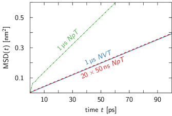
Figure 1: Difference in the mean squared displacements of heuristically unwrapped TIP4P-D water trajectories at constant volume and constant pressure. MD simulations were performed in the $NVT$ and $NpT$ ensembles, respectively, using cubic simulation boxes $(L\approx$2.5\text{\,}\mathrm{nm}$)$, and unwrapped using Gromacs’s trjconv software. The large discrepancy between the constant-volume (solid blue line) and constant-pressure (dash-dotted green line) simulations highlights the shortcomings of the heuristic unwrapping scheme. After splitting the $NpT$ trajectory prior to unwrapping into 20 segments (dashed red line), we obtained MSD values comparable to the $NVT$ results. In these $50\text{\,}\mathrm{ns}$ $NpT$ trajectory segments, particles did not diffuse far enough for unphysical unwrapping to occur.

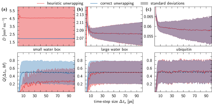
Figure 2: Heuristic unwrapping overestimates the diffusion coefficient in long $NpT$ MD simulations of small systems. Top and bottom panels show the estimated diffusion coefficients $D$ and the fit quality factors $Q$, respectively, from MD simulation trajectories of pure TIP4P-D water in (a) a small box (515 water molecules; $L\approx$2.5\text{\,}\mathrm{nm}$$) and (b) a large box (4139 water molecules; $L\approx$5\text{\,}\mathrm{nm}$$), and (c) of a single ubiquitin molecule in aqueous solution ($L\approx$7.5\text{\,}\mathrm{nm}$$). $D$ and $Q$ are shown as functions of the time-step size $\Delta t_{n}$ used to sub-sample the trajectory in the diffusion analysis.BullerjahnvonBuelow2020 Trajectories were unwrapped at $\Delta t=$1\text{\,}\mathrm{ps}$$ intervals with the correct (blue) and the heuristic (red) unwrapping schemes according to Eqs. (1) and (3), respectively. Lines indicate sample averages. Shaded areas represent one sample standard deviation. We note that in (a) the uncertainty of $D$ from the correct unwrapping scheme is too small to be resolved on the scale of the plot.

In this Communication, we demonstrate that this widely used heuristic trajectory unwrapping scheme is not suitable for simulations at constant pressure $p$. In the $NpT$ ensemble, barostats dynamically adjust the volume of the simulation box to maintain a constant pressure. The particles therefore experience two kinds of displacements: first, their ordinary motion due to collisions and interactions with neighboring particles and, second, a corrective displacement to maintain their relative position inside the box when its volume is varied by the barostat and particle positions are rescaled accordingly. The heuristic unwrapping scheme fails at constant pressure because it uses the current box size to net-reverse all jumps through the periodic boundaries up to the most recent time step, instead of the respective box sizes for each time step where a jump occurred. Repeated failures then result in unphysical amplifications of the corrective displacements, which eventually dominate over the actual particle motion.

A consequence of these shortcomings is depicted in Fig. 1, where we compare MSD estimates from two $1\text{\,}\mathrm{\SIUnitSymbolMicro s}$ MD simulations of TIP4P-D water, which coincide in every aspect except that one was performed in the $NVT$ ensemble, the other in the $NpT$ ensemble (further details of the simulation procedure can be found in the supplementary material). For a few water molecules in the $NpT$ simulation, the heuristic unwrapping scheme caused an unphysical speed-up, which resulted in an overall acceleration of the average MSD when compared to the $NVT$ simulation. Importantly, though, the MSD remained linear after $\approx 3\text{\,}\mathrm{p}\mathrm{s}$. The associated diffusion coefficient was also grossly overestimated, as seen in Fig. 2a, where we compare the heuristically unwrapped $NpT$ data of Fig. 1 to results from a correct unwrapping scheme (see below). Even without a reference value to compare to, the issues of heuristic unwrapping became apparent in our analysis of the quality factor $Q$, which took values significantly below its expected value of $Q\approx 1/2$ for heuristically unwrapped trajectories (see Fig. 2a). The quality factor serves as a measure of how well the data concur with predictions from a minimal diffusive model.BullerjahnvonBuelow2020

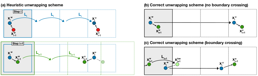
Figure 3: Comparison between the heuristic and correct unwrapping scheme. (a) In a simulation box (blue) with edge length $L_{i}$ at time step $i$, the heuristic unwrapping scheme [Eq. (3)] constructs the unwrapped position $\smash{x^{\text{u}}_{i}}$ from the wrapped coordinate $\smash{x^{\text{w}}_{i}}$ by iterative translation in steps of size $L_{i}$ towards the unwrapped position $\smash{x^{\text{u}}_{i-1}}$ at the previous time step $i-1$, until the condition $\smash{|x^{\text{u}}_{i}-x^{\text{u}}_{i-1}|}\leq L_{i}/2$ is met. However, this can lead to artifacts, as demonstrated at time step $i+1$, where the barostat expands the box to length $L_{i+1}$ (green) and the particle is unwrapped into the wrong box, causing it to move left instead of right, which would be the case if the trajectory were correctly unwrapped via Eq. (1) (faint green circle). (b) Schematic of the correct unwrapping scheme [Eq. (1)]. In situations, where the particle only diffuses within the simulation box, the unwrapped position $\smash{x^{\text{u}}_{i+1}}$ follows from adding the increment $\smash{x^{\text{w}}_{i+1}-x^{\text{w}}_{i}}$ to $\smash{x^{\text{u}}_{i}}$. c) If the particle diffuses out and is placed back into the box according to the PBC, its position $\smash{x_{i+1}^{\text{bw}}}$ before wrapping (“bw”) has to be determined to compute the correct increment to the unwrapped trajectory.

The effects of heuristic unwrapping can be suppressed in various ways, e.g., by shortening the trajectories drastically (Fig. 1), increasing the dimensions of the simulation box (Fig. 2b) or considering molecules that diffuse more slowly (Fig. 2c). This is probably the reason why the above-mentioned shortcomings have gone unnoticed for so long. In the following, we introduce an alternative scheme, sketched in Fig. 3b, that correctly unwraps trajectories from constant-pressure simulations, and use its output as a reference to quantify the errors introduced by the heuristic unwrapping scheme (Fig. 3a). The correct scheme arises naturally when the minimal displacement vector, according to PBC for the instantaneous box geometry, is added to the unwrapped position of the previous time step. This translates into the following evolution equation for the unwrapped positions $x^{\text{u}}_{i}$ in terms of the wrapped positions $x^{\text{w}}_{i}$ and the box width $L_{i}$,

$$x^{\text{u}}_{i+1}=x^{\text{u}}_{i}+(x^{\text{w}}_{i+1}-x^{\text{w}}_{i})-\left\lfloor\frac{x^{\text{w}}_{i+1}-x^{\text{w}}_{i}}{L_{i+1}}+\frac{1}{2}\right\rfloor L_{i+1}\,,$$ (1)

for each spatial dimension in an orthorhombic simulation box. Here, $x^{\text{w}}_{i}$ and $x^{\text{u}}_{i}$ denote the wrapped (“w”) and unwrapped (“u”) one-dimensional coordinates of the particle at time step $i$, respectively. $L_{i}$ is the corresponding box edge length and $\lfloor\cdot\rfloor:\mathbb{R}\to\mathbb{Z}$ is the floor function. In general, we have triclinic boxes of fluctuating size and shape in $NpT$ simulations. The simulation box is then defined by the lattice vectors $\smash{\vec{a}_{k=1,2,3}}$, whose lengths and orientations will fluctuate, with corresponding reciprocal lattice vectors $\smash{\vec{b}_{k}}$ that are obtained by matrix inversion and transposition, $\smash{[\vec{b}_{1}\vec{b}_{2}\vec{b}_{3}]^{T}}=\smash{[\vec{a}_{1}\vec{a}_{2}\vec{a}_{3}]^{-1}}$. We generalize Eq. (1) to triclinic boxes by applying PBC to the displacement vector $\smash{\vec{d}_{i+1}^{\text{w}}}=\smash{\vec{r}^{\text{w}}_{i+1}-\vec{r}^{\text{w}}_{i}}$, i.e.,

$$\vec{d}_{i+1}^{\text{u}}=\vec{d}_{i+1}^{\text{w}}-[\vec{a}_{1}\vec{a}_{2}\vec{a}_{3}]\left\lfloor[\vec{b}_{1}\vec{b}_{2}\vec{b}_{3}]^{T}\vec{d}^{\text{w}}+\left(\begin{array}[]{c}1/2\\ 1/2\\ 1/2\end{array}\right)\right\rfloor\,,$$ (2a)

and adding the resulting vector to the preceding position of the unwrapped trajectory,

$$\vec{r}^{\text{u}}_{i+1}=\vec{r}^{\text{u}}_{i}+\vec{d}^{\text{u}}_{i+1}\,.$$ (2b)

Here, $\smash{\vec{d}_{i+1}^{\text{u}}}$ is calculated according to the instantaneous box size and shape, and the floor function $\lfloor\cdot\rfloor$ is applied component-wise. Note that Eqs. (1) and (2) also apply to the wrapped trajectory displacements $\Delta x_{i}^{\text{w}}=x_{i+1}^{\text{w}}-x_{i}^{\text{w}}$ and $\Delta\vec{r}_{i}^{\text{w}}=\vec{r}_{i+1}^{\text{w}}-\vec{r}_{i}^{\text{w}}$, respectively, which must be unwrapped correctly to eliminate the effects of PBC when used as inputs for the covariance-based diffusion coefficient estimator of Ref. VestergaardBlainey2014, or for other estimators involving the statistics of particle positions or displacements in full Cartesian space.

By contrast, for the commonly used heuristic scheme, we have

$$x^{\text{u}}_{i+1}=x^{\text{w}}_{i+1}-\left\lfloor\frac{x^{\text{w}}_{i+1}-x^{\text{u}}_{i}}{L_{i+1}}+\frac{1}{2}\right\rfloor L_{i+1}\,.$$ (3)

Note that for notational simplicity we concentrate here and in the following on orthorhombic boxes. The difference between the unwrapping schemes defined by Eqs. (1) and (3) appears to be subtle, boiling down to their respective reference points, namely $x^{\text{w}}_{i}$ and $x^{\text{u}}_{i}$. Indeed, we retrieve Eq. (3) if $x^{\text{w}}_{i}$ is replaced with $x^{\text{u}}_{i}$ in Eq. (1). Furthermore, the two schemes coincide exactly when applied to simulations in the $NVT$ ensemble, where $L_{i}\equiv L=\operatorname{\mathit{const.}}$ holds for all $i$.

We illustrate the difference between correct and heuristic unwrapping as defined in Eqs. (1) and (3), respectively, by a one-dimensional (1D) Gaussian model. For this, we consider a Wiener process $x^{\text{w}}$ that evolves on the periodic interval $[-L_{i}/2,L_{i}/2)$. The boundary positions themselves are realizations of a Gaussian white noise $L_{i}$ (a reasonable assumption, as detailed in the supplementary material), which requires us to constantly rescale the position of our process $x^{\text{w}}$ accordingly. The wrapped trajectory within the box thus evolves according to

$$L_{i+1}=\overline{L}+\sigma_{L}S_{i+1}\,,$$ (4a)

$$x^{\text{w}}_{i+1}=\frac{L_{i+1}}{L_{i}}x^{\text{w}}_{i}+\sigma_{x}R_{i+1}-\left\lfloor\frac{x^{\text{w}}_{i}}{L_{i}}+\frac{\sigma_{x}R_{i+1}}{L_{i+1}}+\frac{1}{2}\right\rfloor L_{i+1}\,,$$ (4b)

where $R$ and $S$ denote uncorrelated normal distributed random variables with zero mean and unit variance, satisfying

$$\langle R_{i}\rangle=\langle S_{i}\rangle=0\,, \langle R_{i}R_{j}\rangle=\langle S_{i}S_{j}\rangle=\delta_{i,j}\,.$$

The Kronecker delta $\delta_{i,j}$ evaluates to one if $i=j$ and zero otherwise. Typically, the variance $\sigma_{L}^{2}$ of box fluctuations is not specified in MD simulations, but instead the compressibility $\kappa_{T}$ of the system. Extending our model to three dimensions and assuming isotropic pressure coupling in a cubic box then gives the following approximate relation between the two quantities (see supplementary material),

$$\sigma_{L}^{2}\mathop{\approx}^{\sigma_{L}\ll\overline{L}}\kappa_{T}(9\beta\overline{L})^{-1}\,.$$ (5)

Here, $\beta=(k_{\text{B}}T)^{-1}$ is the inverse thermal energy scale, $T$ the absolute temperature and $k_{\text{B}}$ the Boltzmann constant.

We generated trajectories for different values of $\smash{\overline{L}}$, $\smash{\sigma_{L}^{2}}$ and $\smash{\sigma_{x}^{2}}$, where the latter coincides (up to a numerical prefactor $2\Delta t$ for some time-step size $\Delta t$) with the one-dimensional diffusion coefficient $D_{NVT}$ observed in the $NVT$ ensemble. Each trajectory was unwrapped via both schemes, and for the resulting time series we calculated and fitted the corresponding MSD values using the procedure described in Ref. BullerjahnvonBuelow2020, to extract estimates $\sigma^{2}$ for the effective diffusion coefficient. Intriguingly, we discovered for our correct unwrapping scheme [Eq. (1)] that box fluctuations do not only add static noise to the MSD, resulting in a constant shift of the MSD curve, but also affect its slope (see supplementary material). In most practical cases, however, this correction is minuscule and can be neglected.

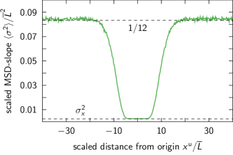
Figure 4: Local estimates of the effective diffusion coefficient $\sigma^{2}$ as a function of the particle’s unwrapped position $x^{\text{u}}$. For 1000 heuristically unwrapped trajectories of length $N=$5\text{\times}{10}^{5}\text{\,}$$, we used Eq. (6) to determine how the sample average $\langle\sigma^{2}\rangle$ gradually deviates from its expected value $\sigma_{x}^{2}$ as the particle diffuses further from its starting point. The wrapped trajectories were generated via Eqs. (4) using the simulation parameters $\overline{L}=1.0$, $\sigma_{x}=0.05$ and $\sigma_{L}=0.02$. The two horizontal dashed lines indicate the actual diffusion coefficient $\sigma^{2}=\sigma^{2}_{x}$ and the asymptotic limit expected for heuristic unwrapping, $\sigma^{2}=\smash{\overline{L}^{2}}/12$, respectively.

For the heuristic scheme [Eq. (3)], we observed a gradual increase in the value of the estimated $\sigma^{2}$ as the particle’s unwrapped position deviated further from its origin. To characterize this effect, we considered very short segments of the unwrapped trajectories, which gave us local estimates

$$\sigma^{2}(x^{\text{u}}_{i}=x^{\text{u}})=(x^{\text{u}}_{i+2}-x^{\text{u}}_{i})^{2}-(x^{\text{u}}_{i+1}-x^{\text{u}}_{i})^{2}$$ (6)

of the diffusion coefficient for every instance where the trajectories reached $x^{\text{u}}$. Figure 4 shows the sample average over these estimates for bins of width $\smash{\overline{L}/5}$, where $\smash{\sigma^{2}(-5<x^{\text{u}}<5)}\approx\sigma_{x}^{2}$. Further away from the original simulation box $\sigma^{2}$ rises sharply, up to the point where the heuristic unwrapping scheme essentially places the particle randomly inside the interval $\left[x^{\text{u}}_{i}-L_{i+1}/2,x^{\text{u}}_{i}+L_{i+1}/2\right)$ at time step $i+1$. This causes $\sigma^{2}$ to plateau at

$$\sigma^{2}(x^{\text{u}}\to\pm\infty)\approx\overline{L}^{2}/12\,,$$

which coincides with the variance of a uniform distribution on $\left[x^{\text{u}}_{i}-L_{i+1}/2,x^{\text{u}}_{i}+L_{i+1}/2\right)$ for all $x^{\text{u}}_{i}$. Note that the asymptotes of $\sigma^{2}$ are independent of $\sigma_{L}$.

Figure 4 highlights the fact that errors induced by the heuristic unwrapping scheme remain moderate as long as the particles of interest do not diffuse too far from the original simulation box in the course of the simulation. The question thus arises whether one can quantify a critical simulation time, beyond which sizable errors in the diffusion coefficient are to be expected? According to our simulations, this time seems to be on the same order as the average time it takes the heuristic unwrapping scheme to cause a divergent unwrapping event, where the particle is unwrapped into the wrong simulation box, as depicted in Fig. 3a, for the first time. We roughly estimated this time with the help of the probability to observe a divergent event at time $i\Delta t$, where $\Delta t$ is the time between consecutive structures to be unwrapped. As detailed in the supplementary material, we find the following approximate closed-form expression for the critical simulation time,

$$t_{\text{crit}}\approx\frac{9\beta\overline{L}^{5}}{50\kappa_{T}D_{NVT}[W_{0}(C^{2/5})]^{2}}$$ (7)

with $C=\smash{9dN_{\text{p}}\beta\overline{L}^{5}/\left(25\sqrt{5\pi}\kappa_{T}D_{NVT}\Delta t\right)}$. Here, $d$ denotes the dimension of the simulation box, $N_{\text{p}}$ is the number of diffusing particles of interest in the simulation, and $W_{0}(z)$ is the principal branch of the Lambert $W$ function. For large arguments, the latter can be replaced with the first two terms of its Taylor expansion, namely

$$W_{0}(z\gg 1)\approx\ln(z)-\ln\left(\ln(z)\right)+\mathcal{O}\left(\frac{\ln\left(\ln(z)\right)}{\ln(z)}\right)\,.$$

In general, $D_{NVT}$ is unknown, but practitioners can instead use their estimate of $D_{NpT}$. This results in a slightly more conservative value for $t_{\text{crit}}$, since $D_{NpT}>D_{NVT}$ for heuristically unwrapped trajectories. For bulk water at ambient conditions, we have experimental values of $D=$2.3\text{\,}{\mathrm{nm}}^{2}\text{\,}{\mathrm{ns}}^{-1}$$,KrynickiGreen1978 $\kappa_{T}=$4.5\text{\times}{10}^{-10}\text{\,}{\mathrm{Pa}}^{-1}$$,Kell1970 and a number density of $\smash{N_{\text{p}}/\overline{L}^{3}}\approx$33.3\text{\,}{\mathrm{nm}}^{-3}$$. We then have to a good approximation $t_{\text{crit}}\approx($0.0061\text{\,}\mathrm{ns}$)\smash{N_{\text{p}}^{3/2}}\smash{[\Delta t/($1\text{\,}\mathrm{ps}$)]^{0.081}}$ for water molecule numbers in the range of $10^{3}<N_{\text{p}}<10^{6}$ and time-step sizes in the range of $$0.1\text{\,}\mathrm{ps}$<\Delta t<$10\text{\,}\mathrm{ps}$$. For boxes with $N_{\text{p}}=570$, 2900 and 14000 water molecules and $\Delta t=$1\text{\,}\mathrm{p}\mathrm{s}$$, the critical times for water self-diffusion calculations are $t_{\text{crit}}\approx 0.1$, 1 and $10\text{\,}\mathrm{\SIUnitSymbolMicro s}$, respectively.

Figure 5: Relative error in the diffusion coefficient as a result of heuristic unwrapping depending on the duration of the simulation. The relative difference between $D_{NpT}$ and $D_{NVT}$ obtained from heuristically unwrapped trajectories is shown for the 1D-Gaussian model (solid green line) and the TIP4P-D water data underlying Figs. 1 and 2a (gray dashed line). The diffusion coefficient $D_{NpT}$ was estimated using the formalism of Ref. BullerjahnvonBuelow2020, with $\Delta t_{n}=\Delta t_{\text{opt}}=$10\text{\,}\mathrm{ps}$$ and $M=5$. Lines indicate sample averages. The 1D-Gaussian model and the critical time $t_{\text{crit}}$ [Eq. (7), black dashed line] were evaluated using the parameters $\smash{\overline{L}}=$2.49\text{\,}\mathrm{nm}$$, $\kappa_{T}=\smash{$4.5\text{\times}{10}^{-10}\text{\,}{\mathrm{Pa}}^{-1}$}$ (corresponding to $\sigma_{L}=$0.0092\text{\,}\mathrm{nm}$$), $D_{NVT}=\smash{$1.95\text{\,}{\mathrm{nm}}^{2}\text{\,}{\mathrm{ns}}^{-1}$}$, $d=3$ and $N_{\text{p}}=515$, which were either directly read off the MD simulation files or extracted from the correctly unwrapped trajectories. All trajectories were unwrapped using a time-step size of $\Delta t=$2\text{\,}\mathrm{ps}$$. At short simulation times ($\lesssim$160\text{\,}\mathrm{ns}$$), the relative error for the TIP4P-D water data fluctuates around zero and was therefore omitted from the plot.

To test our estimate of the critical time $t_{\text{crit}}$ after which we expect the heuristic scheme to fail, we reexamined the heuristically unwrapped TIP4P-D water trajectories from the smaller simulation box (see Fig. 2a) by truncating them at different points. We then determined how the resulting effective diffusion coefficient $D_{NpT}$ varies with the length $N$ of the unwrapped trajectory. In this calculation of $D_{NpT}$, we used a time-step size of $\Delta t_{n}=\Delta t_{\text{opt}}=$10\text{\,}\mathrm{ps}$$, as described in Ref. BullerjahnvonBuelow2020, , to suppress nonlinearities in the MSD on short time scales. While the trajectories of Figs. 1 and 2 were unwrapped using a time-step size of $\Delta t=$1\text{\,}\mathrm{ps}$$, we chose here $\Delta t=$2\text{\,}\mathrm{ps}$$ to suppress the effect of box-fluctuation correlations (see supplementary material), which we do not account for in the 1D-Gaussian model. Our results are presented in Fig. 5, next to corresponding synthetic three-dimensional data generated by our 1D-Gaussian model [Eq. (4)]. The critical time, according to Eq. (7), provides a reasonable estimate of the run length, beyond which incorrect heuristic unwrapping events cause significant errors for both the MD data the 1D-Gaussian model. Further simulations using our 1D-Gaussian model confirm the validity of Eq. (7) for a broad range of simulation parameters (see supplementary material). We therefore advise practitioners to calculate $t_{\text{crit}}$ and compare it to their simulation time if they suspect that the heuristic unwrapping scheme has affected their results in the past.

In this Communication, we have provided extensive evidence to show that the heuristic unwrapping scheme, as implemented in popular simulation and visualization software, is not appropriate for MD simulations in the $NpT$ ensemble. Initially, its use causes only negligible deviations from the correctly unwrapped trajectory, but, as the simulation progresses, divergent unwrapping events (Fig. 3a) eventually set in that result in a significant overestimation of diffusion coefficients. This is especially evident for fast diffusing molecules in small simulation boxes, as seen in our MD simulation of TIP4P-D water (Figs. 1 and 2a). In the future, the increasing performance of highly parallel GPU architectures will steadily extend the time scales covered by MD simulations, which will increase the chance of noticeable errors in the diffusion coefficient estimated from incorrectly unwrapped trajectories. By applying PBC on the displacement vector at each time step according to the instantaneous box geometry, the correct unwrapping scheme in Eqs. (1) and (2) circumvents the errors arising from the use of the heuristic scheme. In principle, Cartesian-space particle displacements could also be collected “on the fly” at the discrete steps of time integration and barostatting, summed for, say, $1\text{\,}\mathrm{ps}$, and then saved for subsequent analysis. However, trajectory unwrapping not only allows us to reconstruct the aggregate particle displacements with minimal assumptions, but also to (re)analyze trajectories from standard MD codes. Going forward, we urge that the correct unwrapping scheme be implemented in the standard simulation-analysis packages.

Supplementary material

See the supplementary material for details on MD simulation procedures, an analysis of box-volume fluctuations in simulations of TIP4P-D water, a numerical and analytic study of the MSD of a correctly unwrapped trajectory, and a detailed derivation of the critical simulation time estimate, along with simulation results to test its validity for various parameter combinations.

Data availability

The data that support the findings of this study are available from the corresponding author upon reasonable request.

- (1) C. L. Vestergaard, P. C. Blainey, and H. Flyvbjerg, Optimal estimation of diffusion coefficients from single-particle trajectories, Phys. Rev. E 89, 022726 (2014).
- (2) J. T. Bullerjahn, S. von Bülow, and G. Hummer, Optimal estimates of diffusion coefficients from molecular dynamics simulations, J. Phys. Chem. XXX, YYY-ZZZ (2020).
- (3) T. Giorgino, J. Henin, J. Hoermann, O. Lenz, C. Mura, D. M. Rogers, and J. Saam, VMD PBCTools plugin, version 3.0, https://github.com/frobnitzem/pbctools.
- (4) M. J. Abraham, T. Murtola, R. Schulz, S. Páll, J. C. Smith, B. Hess, and E. Lindahl, GROMACS: High performance molecular simulations through multi-level parallelism from laptops to supercomputers, SoftwareX 1-2, 19-25 (2015).
- (5) D. A. Case, I. Y. Ben-Shalom, S. R. Brozell, D. S. Cerutti, T. E. Cheatham III, V. W. D. Cruzeiro, T. A. Darden, R. E. Duke, D. Ghoreishi, M. K. Gilson, H. Gohlke, A. W. Goetz, D. Greene, R. Harris, N. Homeyer, Y. Huang, S. Izadi, A. Kovalenko, T. Kurtzman, T. S. Lee, S. LeGrand, P. Li, C. Lin, J. Liu, T. Luchko, R. Luo, D. J. Mermelstein, K. M. Merz, Y. Miao, G. Monard, C. Nguyen, H. Nguyen, I. Omelyan, A. Onufriev, F. Pan, R. Qi, D. R. Roe, A. Roitberg, C. Sagui, S. Schott-Verdugo, J. Shen, C. L. Simmerling, J. Smith, R. Salomon-Ferrer, J. Swails, R. C. Walker, J. Wang, H. Wei, R. M. Wolf, X. Wu, L. Xiao, D. M. York, and P. A. Kollman, AMBER 2018, University of San Francisco (2018).
- (6) K. Krynicki, C. D. Green, and D. W. Sawyer, Pressure and temperature dependence of self-diffusion in water, Faraday Discuss. Chem. Soc. 66, 199-208 (1978).
- (7) G. S. Kell, Isothermal compressibility of liquid water at 1 atm, J. Chem. Eng. Data 15, 119-122 (1970).