Territorial Behaviour of Buzzards versus
Random Matrix Spacing Distributions

Abstract.

A deeper understanding of the processes underlying the distribution of animals in space is crucial for both basic and applied ecology. The Common buzzard (Buteo buteo) is a highly aggressive, territorial bird of prey that interacts strongly with its intra- and interspecific competitors. We propose and use random matrix theory to quantify the strength and range of repulsion as a function of the buzzard population density, thus providing a novel approach to model density dependence. As an indicator of territorial behaviour, we perform a large-scale analysis of the distribution of buzzard nests in an area of $300$ square kilometres around the Teutoburger Wald, Germany, as gathered over a period of $20$ years. The nearest and next-to-nearest neighbour spacing distribution between nests is compared to the two-dimensional Poisson distribution, originating from uncorrelated random variables, to the complex eigenvalues of random matrices, which are strongly correlated, and to a two-dimensional Coulomb gas interpolating between these two. A one-parameter fit to a time-moving average reveals a significant increase of repulsion between neighbouring nests, as a function of the observed increase in absolute population density over the monitored period of time, thereby proving an unexpected yet simple model for density-dependent spacing of predator territories. A similar effect is obtained for next-to-nearest neighbours, albeit with weaker repulsion, indicating a short-range interaction. Our results show that random matrix theory might be useful in the context of population ecology.

1. Introduction

It is one of the major goals of population ecology, and indeed one of the oldest goals of ecology as a whole, to understand the processes that govern the distribution of animals in space and time [24]. This is not only an important academic question, but has crucial implications for conservation planning and management [21, 31]. Birds of prey, or raptors, are often apex predators, are among the most-threatened groups of birds globally [23], and their abundance and diversity is a key indicator of the state of the ecosystem as a whole [35]. Birds of prey have been used as model systems in other such contexts, for example vultures, including the interaction with humans [14], or even as an indicator for the well-being of entire ecosystems [21, 31]. Their charismatic nature, conspicuousness and relatively high vulnerability due to their trophic position increases their conservation value [35] and hence the recording of their population dynamics has attracted a lot of attention for centuries [30]. In this article, we focus on the behaviour of such a territorial bird of prey, the common buzzard, and model a change in its population density over $20$ years. As we shall see, their territoriality, measured by the repulsion among their nests, increases significantly with population size.

In many animal and plant populations, reproductive success decreases with increasing population density. This density dependence of reproduction has been known since the dawn of modern animal ecology [24]. Although density dependence has been examined in different taxa [37], it is rather easily studied in large, territorial species. One particularly prominent group used for disentangling hypotheses about density-dependent processes have been birds of prey [21, 22]. Their predatory habit could amplify the occurrence of strong density dependence and make them especially suited for studies of the underlying mechanisms [11]. Territoriality allows density effects to be examined in detail, while this possibility could be impaired in classically colonial species. Birds of prey also offer the advantage of being very site-faithful: once they have occupied a territory, they rarely move and they are highly aggressive against intruders and hence territorial aggression can be fatal. The study of mechanisms that could explain the spatial clustering of bird of prey territories is therefore of theoretical as well as applied value.

Here, the locations of buzzard nests collected over the $20$ years $2000\!-\!2019$ in the Teutoburger Wald around Bielefeld, Germany, are investigated. We are in the comfortable position to have about $100-200$ nests per year available in this approximately two dimensional (2D) landscape, over a period of $20$ years; see Section 2 for details. Given such a data set, it is tempting to model the emergence and behaviour in space and time from an ecological angle. However, this would require to make many assumptions and to introduce even more parameters, which bears the danger of overfitting. Indeed, a less biased approach would begin by extracting structural properties from the data, such as distribution patterns, distance preferences, or any kinds of correlations in space and time. Although the inference point of view from point process theory would be natural, compare [19], the data set does not seem to be large enough for such an endeavour. Consequently, the goal of this initial approach is rather modest in the sense that we primarily look at the spacing distribution between neighbouring points, that is, the nest locations, in order to test whether a model with one parameter and no a priori biological assumptions could still explain the change in territorial spacing over time.

A popular approach to spacing distributions is based on random matrix ensembles. They allow to analytically quantify the repulsion among data points, without making further assumptions. In particular, the spacing distributions of the classical random matrix ensembles in one (1D) and two dimensions (2D) are parameter free. For some details on random matrices, we refer to Appendix A. Their history started independently in multivariate statistics [39], inspired from agriculture by Wishart, and in a statistical theory of energy levels of complex quantum systems by Dyson [12], motivated by Wigner and ideas of Bohr about the compound nucleus; see [17] for a historic account and various modern applications. Further examples without quantum mechanical background repeatedly show the signature of random matrix statistics, such as the spacing between subsequent buses in Cuernavaca (Mexico) [20], and parked cars [32, 1] or birds on a power line [34]. While most comparisons are made for data in 1D, comparing with the statistics of real eigenvalues of symmetric or Hermitian random matrices, few examples exist in 2D. Here, one is comparing with complex eigenvalues of random matrices without symmetries, with applications ranging from quantum chaotic systems with dissipation [16, 2] over quantum field theory with chemical potential [28] to the spacing between chief towns of departments or districts [27] and Swedish pine trees [26]. Data sets similar to the latter two have been modelled by so-called determinantal point processes [25], for which random matrices provide a particular example. A novel feature we propose here is to track the time evolution of the repulsion strength, in this case as a function of the population density. This allows us to draw biologically more relevant conclusions, compared to the static distribution of birds on a power line.

In order to apply such ideas to the distribution of nests, we employ recent progress on the universality of certain distributions in random matrix theory. In Section 3, we start with a comparison to the distribution from a uniform Poisson process in 2D, which describes the distribution of uncorrelated points, and to the distribution of the complex Ginibre ensemble of random matrices [15], which displays a rather strong repulsion. The repulsive nature is also easily detectable from the diffuse scattering components in the diffraction image of random point sets in 2D [5]. We stress again that both distributions are parameter free, after fixing the normalisation and first moment to unity. As we shall see, the nest locations are indeed not adequately described by a Poisson process, in line with the known and frequently observed territorial repulsion of the buzzards.

In this first step, it also becomes clear that the repulsion in the Ginibre process is too strong, which is perhaps not too surprising either, as the ecological system should show some repulsion on a shorter scale (visual range), but not a long-range one. To deal with this situation, we embark on a simple one-parameter interpolation between Poisson and Ginibre statistics, which we derive from a known 2D Coulomb gas ensemble at variable temperature (being a non-determinantal, general Gibbs point process [13, 36]). Since the underlying model has no direct meaning in the biological system, the parameter $\beta$ (proportional to the inverse temperature) is just taken as an effective phenomenological quantity and then determined by a simple fitting procedure. It directly measures the power of local repulsion of two points at distance $s$, which is proportional to $s^{\beta+1}$.

It turns out that the employed one-parameter family of spacing distributions works well for the data. Moreover, our effective parameter proves sensitive to population density dependent properties in time, which indicates its suitability for our initial step in the data analysis. In Section 3, we explain how we analyse our data in moving time averages, with further details provided in Appendix C. Our conclusions and open questions are summarised in Section 4.

2. Object of Study, Density Dependence, and Territoriality

The Common buzzard (Buteo buteo L.) is a medium-sized bird of prey ($50\!-\!57$ cm body length, $525\!-\!1364$ g body weight) and breeds across the Palaearctic [10]. Its main prey consists of microtine rodents. A Common buzzard population comprising between 63 and 266 breeding pairs per year was monitored from $2000$ to $2019$ in an investigation area in Germany. The $300$ km² area (8^∘25’E and 52^∘6’N) is located in Eastern Westphalia and consists of two $125$ km² grid squares and $50$ km² edge areas. The main habitat is the Teutoburger Wald, a low mountain region reaching a height of $315$ m above sea level. Ridges are covered by Norway Spruce Picea abies and Beech Fagus sylvatica, with Oak Quercus robur and Q. petrea forests at lower altitudes. The second main habitat is a cultivated landscape to the north and south. In the north, forests are composed mainly of Beech and Oak, whereas Scots Pine Pinus sylvestris dominates in the south. The size of forest patches varies from rows of trees to large patches of more than $10$ km² in size, and about $17\%$ of the study site is forested. Most forests are less than 100 years old and the spruce forests are atypical of this region. This study site has been intensively monitored for Common buzzard and the resulting spatial data have been used extensively before [21, 9, 29]. We use the very same data of the nest locations for our analysis, completed by the most recent years.

All forest patches were visited in late winter to look for breeding pairs and all nests of four raptor species (Common buzzard, Goshawk Accipiter gentilis, Red Kite Milvus milvus and Honey Buzzard Pernis apivorus) were recorded in either large-scale maps or GPS devices to examine spatial distribution and interspecific competition. When an incubating Common buzzard was observed on the nest in both March and April, that pair was classified as breeding (in contrast to non-breeders which did not occupy a nest). An illustration is shown in the left panel of Figure 1.

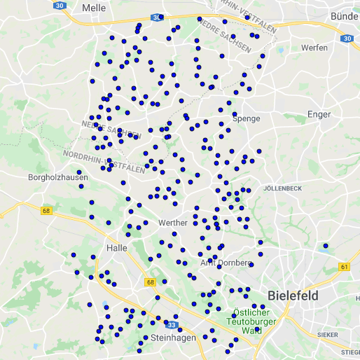
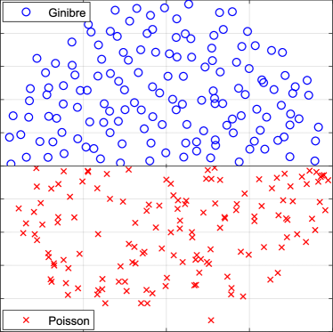
Figure 1. Visual comparison of nest locations of the Common buzzard with a typical snapshot of random matrix eigenvalues.
Left: Map showing the locations of $251$ observed buzzard nests from the year $2019$ north-west of Bielefeld. Note how smaller cities like Halle and Werther coincide with holes in the data. There are more nests outside the cluster shown here, but the positions of these have not been recorded.
Right: Points distributed according to the 2D Poisson distribution (bottom, red crosses) and eigenvalues of a large complex Ginibre matrix (top, blue circles). Both ensembles consist of $300$ points, the Poisson variables are generated uniformly on the unit disk, while the Ginibre variables are the eigenvalues of a complex Gaussian random matrix normalised to the unit disk. Only the top/bottom half disk is shown for an easier comparison. Notice how the Poisson points tend to cluster, whereas points from the Ginibre ensemble are more evenly spaced. This is reflected in the nearest neighbour spacing distributions (A.1) and (A.4), which we compare quantitatively to the buzzard nests below.

Figure 1 shows the nest locations for a single year $2019$, where the population density is among the highest over the observed period. The effect of towns and smaller cities appears to be visible as holes in the data set. The statistics on the potential edge effects is too small to draw conclusions. We thus chose to treat all the data points as being part of a bulk, without considering edge effects. Notice that, within the Ginibre ensemble of random matrices, the statistics at the edge of the spectrum (unit disk) differs from that of the bulk points. There, the transition from edge to bulk is very rapid though, within a distance of order $1/\sqrt{N}$ from the edge for $N$ points; compare [38] for the mathematical discussion of this class of random matrices.

2019 alone                          2015-2019                          All Years
Nearest Neighbour
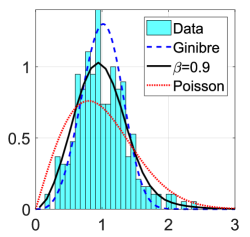
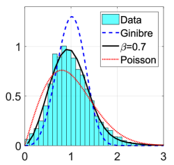
Next-to-Nearest

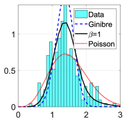
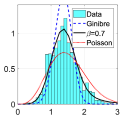
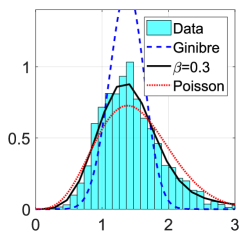
Figure 2. Comparison of distances between nests to those of a 2D Coulomb gas (A.3) with a Kolmogorov fit, both nearest neighbour (NN, top row) and next-to-nearest neighbour (NNN, bottom row), where the repulsion $\beta$ is treated as a fitting parameter. We have also added the curves corresponding to the analytic expressions for Poisson and Ginibre variables; see Eqs. (A.1) and (A.4) for the top row, and Eqs. (A.2) and (A.5) for the bottom row. To illustrate our grouping of several years explained in the main text, we provide the fit of a single year (left column), of $5$ years (middle column), and of all $20$ years (right column). Using one year, the fit quality is rather poor, but when using all years, we lose the temporal information. We therefore make the compromise of moving averages of $5$ years. The result is shown in Figure 3. See also Figure 4 in Appendix C for the effects of different group sizes.

3. Territorial Behaviour of Common Buzzards

Ideally, we wish to investigate the territorial behaviour over the years. Unfortunately, the individual years have too few data points for comparison, as typically of the order of $1000$ data points would be needed to make a good fit; see Figure 2 (left) and Figure 4 (left) in Appendix C. We therefore group the nests in ensembles of $5$ years ($2000\!-\!2004$, $2002\!-\!2005$, …) as follows. For each year, the spacings are determined individually and then put into an ensemble. After unfolding the data points as explained in Appendix B, we fit the nearest and next-to-nearest neighbour spacings of every ensemble to a Coulomb gas, with $\beta$ as the fitting parameter describing the local repulsion; see Figures 2 and 3. Notably, these fits to NN and NNN do not give the same value for $\beta$ within the same ensemble. Let us first compare the $\beta$-dependence within each ensemble. Initially, the next-to-nearest neighbour spacing gives a significantly lower value for $\beta$, which is about half of that of the nearest neighbour $\beta$-value. At first, it is close to the Poisson process at $\beta=0$. This suggests that the correlation length is relatively small: the buzzards are aware of their direct neighbours, but do not have long-range interactions. This differs from the long-range interaction of the Coulomb force.

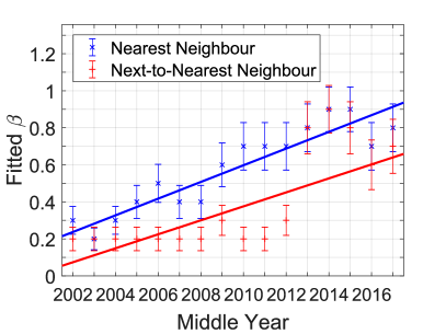
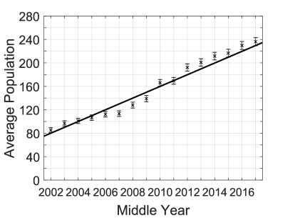
Figure 3. Left: Comparison of the NN spacing distribution of all collected nests $2000-2019$ to a Kolmogorov fit for the effective parameter $\beta$ of the spacing distribution, obtained from a 2D Coulomb gas (A.3); see Appendix A. The fits to nearest (top blue data points) and NNN spacing (bottom red data points) are made in groups of $5$ years. That is, the first group is $2000-2004$ and the last is $2015-2019$; compare with Figure 4 in Appendix C discussing different groups sizes.
As detailed in Appendix C, the statistical error bars are found by fitting the parameter $\beta$ in the spacing distribution obtained numerically from the Coulomb gas (A.3) to themselves (bootstrapping), that is, the spread of the $\beta$ obtained by fitting each of the $10^{4}$ realisations to their average distribution. To avoid any influence from the choice of bin width for our data, we have in fact fitted to the cumulative distribution of the spacing distributions, using the Kolmogorov distance. A least-squares fit with a straight line is provided for both spacing distributions, to show the trend.
Right: The averages of the population size over the same groups of $5$ years as well as a fit with a straight line. The errors of the individual years are here assumed Poissonian and propagated to the averages. Note that the linear increase in size coincides with the increase in $\beta$.

Next, we also compare the growth in population in Figure 3 (right) to the time dependence of the repulsion measured in $\beta$ in Figure 3 (left) over the years and find that an increase in population coincides with an increase in repulsion. This is indicated by the linear fits in Figure 3. Note that the observed area is roughly the same through the years, so the population is proportional to the density. Surprisingly, beyond a certain critical density, the $\beta$-value of both spacings becomes comparable, indicating an increase in correlation length. For Coulomb gases, the normalised spacing distribution is invariant under a change in density, but here the added population makes the Common buzzards more territorial. This suggests that they care only about their closest neighbours, but not about the overall scale of the environment. In other words, there exists a length scale that is not present in the global potential of the Coulomb gas.

4. Conclusion and Open Questions

Above, we compared the spacing distributions of the nests of the Common buzzard in an area of the Teutoburger Wald to a one-parameter family of correlated random variables that includes the behaviour of Poisson random variables and of complex eigenvalues of random matrices in limiting cases. We find that it provides a good effective description of the repulsion among neighbouring nests, thus quantifying the territorial interaction between the birds. This allows us to isolate population density effects over time, where we find an increase in repulsion through an increase of absolute population density, and to also gauge the correlation length of the interactions. We observe that the Common buzzard seems to care more about nearest neighbours, while next-to-nearest neighbours only become important beyond a certain population density.

One of the open questions is to come up with a simple phenomenological model that would lead to similar statistics as the one-parameter family of a 2D Coulomb gas that we found to be effective in our data analysis. In a more theoretical direction, the explicit data analysis has shown that the theoretical results from [2] needed to be extended in several directions, to include longer range correlations and to efficiently deal with small data sets. This will certainly inspire future activities on the mathematical side as well, for instance to include different charges to model several species.

Acknowledgements: This paper grew out of a collaboration between members of three distinct research groups, all supported by the German Science Foundation (DFG), namely CRC1283 “Taming uncertainty and profiting from randomness and low regularity in analysis, stochastics and their applications” (GA and MB), IRTG2235 “Searching for the regular in the irregular: Analysis of singular and random systems” (AM), and CRC/Transregio 212 “A Novel Synthesis of Individualisation across Behaviour, Ecology and Evolution: Niche Choice, Niche Conformance, Niche Construction (NC)³” (OK). We thank Ellen Baake for useful discussions and careful comments on the manuscript, as well as the School of Mathematics and Statistics of the University of Melbourne for hospitality (G.A.).

Appendix A Spacing Distributions from Poisson, Ginibre and Coulomb Gas

Here, we recall the spacing distributions between nearest and next-to-nearest neighbours of correlated and uncorrelated random variables and discuss their relevance, related to the concept of universality in random matrix theory.

Let us begin with the uncorrelated case, the Poisson distribution (Poi). Given a set of uniformly distributed, uncorrelated points in 2D, the distances between nearest neighbours (NNs) and next-to-nearest neighbours (NNNs) follow the respective spacing distributions

(A.1) $$p_{\mathrm{Poi}}^{\mathrm{(NN)}}(s)\; =\;\frac{\pi}{2}s\ \mathrm{e}^{-\pi s^{2}/4},$$

(A.2) $$p_{\mathrm{Poi}}^{\mathrm{(NNN)}}(s)\; =\;\frac{\pi^{2}}{8}s^{3}\ \mathrm{e}^{-\pi s^{2}/4},$$

in the limit of large data sets. Here, both the zeroth and first moments are normalised to 1. Note that in contrast to 1D, where the Poisson distribution for NN is the simple exponential $\mathrm{e}^{-s}$, without repulsion among NN, uncorrelated points in 2D also seem to repel each other, with the linear factor stemming from the 2D area measure. The derivation of Eq. (A.1) is standard. Computing the probability that the NNs of a given point lie in a ring of radius $s$ and thickness d$s$, with all other points being outside that ring, leads to (A.1) in the limit of large particle numbers. The computation of NNN in (A.2) merely uses independence and (A.1), where we refer to Appendix A in [33] for a derivation in arbitrary dimensions, including higher-order neighbours.

Let us turn to the spatial statistics based on random matrices. They have been conceived as a null model, for instance in the analysis of multiple time series. In that case, the data matrix with several measured times series of equal length as rows is replaced by a random matrix with independent Gaussian entries, with zero mean and unit variance. Taking this matrix times its transposed we obtain a positive definite matrix, the Wishart matrix, and precise analytic statements about the eigenvalues of this matrix can be made [13]. The eigenvalues become strongly coupled, due to the Jacobi determinant from the transformation that diagonalises the Wishart matrix. In the limit of large matrix size, these results become universal, that is, they hold for a much larger class of random matrix entries. In many instances, the majority of eigenvalues obtained from the matrix of time series is well described by those of the random matrix, after proper rescaling. Further applications of the universal random matrix predictions to data that are not necessarily eigenvalues of a matrix or an operator are mentioned in the Introduction.

In order study complex eigenvalues, we consider $N\times N$ complex, non-Hermitian random matrices, with independent entries drawn from the complex normal distribution, the complex Ginibre (Gin) ensemble [15]. We directly consider the random matrix now, without multiplying by its Hermitian conjugate, and thus its eigenvalues are complex. As for the real eigenvalues above, the complex eigenvalues of such matrices become correlated random variables, due to the Jacobi determinant of the Schur decomposition. The joint density of complex eigenvalues reads [15]

(A.3) $$p_{\mathrm{Cou},\beta}(z_{1},\ldots,z_{N})\;\propto\;\exp\biggl{(}\beta\sum_{1\leq j<k\leq N}\log|z_{k}-z_{j}|-\sum_{\ell=1}^{N}|z_{\ell}|^{2}\biggr{)},$$

with $\beta=2$. It equals the static gas of $N$ charged particles at the locations of the complex eigenvalues, repelling each other with respect to the long-range 2D Coulomb (Cou) interaction at a specific inverse temperature $\beta=(k_{B}T)^{-1}$, with $k_{B}$ the Boltzmann constant. The particles (eigenvalues) are kept together through a confining, quadratic potential $V(z)=|z|^{2}$, that originates from the Gaussian distribution of matrix elements in the Ginibre ensemble. Compared to standard conventions for the Gibbs measure in statistical mechanics, we have rescaled the positions as $\beta|z_{j}|^{2}\to|z_{j}|^{2}$, allowing us to take the limit $\beta\to 0$ below.

The limiting NN and NNN spacing distributions among complex eigenvalues with joint distribution (A.3) at $\beta=2$ can be derived explicitly in the large-$N$ limit:

(A.4) $$p^{\mathrm{(NN)}}_{\mathrm{Gin}}(s)\; =\;\left(\prod_{k=1}^{\infty}\frac{\Gamma(1+k,s^{2})}{k!}\right)\sum_{j=1}^{\infty}\frac{2s^{2j+1}\mathrm{e}^{-s^{2}}}{\Gamma(1+j,s^{2})},$$

(A.5) $$p^{\mathrm{(NNN)}}_{\mathrm{Gin}}(s)\; =\;\left(\prod_{k=1}^{\infty}\frac{\Gamma(1+k,s^{2})}{k!}\right)\sum_{j=1}^{\infty}\sum_{\begin{subarray}{c}k=1\\ k\neq j\end{subarray}}^{\infty}\frac{\gamma(1+j,s^{2})}{\Gamma(1+j,s^{2})}\frac{2s^{2k+1}\mathrm{e}^{-s^{2}}}{\Gamma(1+k,s^{2})}.$$

Here, $\Gamma(1+k,s^{2})=\int_{s^{2}}^{\infty}t^{k}\mathrm{e}^{-t}\mathrm{d}t$ and $\gamma(1+k,s^{2})=\int^{s^{2}}_{0}t^{k}\mathrm{e}^{-t}\mathrm{d}t$ are the incomplete Gamma functions. The exact expressions at finite matrix size, where sums and products are truncated at $N-1$, converge very rapidly. The derivation for NN (A.4) from [16] can be sketched as follows. Placing one eigenvalue by hand at the origin, for instance by setting $z_{1}=0$ in (A.3), the gap probability that all other eigenvalues are at least at radial distance $s$ is obtained by integrating the joint density (A.3) over all angles and over all radii larger than $s$. Algebraic manipulations lead to the gap probability, being equal to the product in front of the sum in (A.4). A differentiation with respect to $s$ then gives the spacing distribution. The same idea leads to the NNN expression (A.5) or higher order spacings. The generating function for the corresponding gap probability was calculated in [3], and a short computation leads to (A.5).

Let us discuss some properties of the spacing distributions in (A.4) and (A.5). It is not difficult to see that, for small arguments, the repulsion is much stronger in the Ginibre ensemble, being proportional to $s^{3}$ for NN in (A.4), and to $s^{5}$ for NNN in (A.5), compared to (A.1) and (A.2) in the Poisson case, respectively; compare Figure 2. For simplicity, we have not yet rescaled the expressions in (A.4) and (A.5) by the respective first moments, as it is done in Figure 2 for comparison to data. Both distributions for NN and NNN in the Ginibre ensemble are universal, in the sense that they hold beyond independent Gaussian distributions for the matrix elements; see [4, 38] for the precise statements of the theorems for different generalisations. Moreover, for all three Ginibre ensembles with real, complex, or quaternion matrix elements, the spacing distributions in the bulk all agree [2, 7], which is why we display a single distribution for the Ginibre ensemble in Figure 2. This is in sharp contrast to Hermitian random matrices with real, complex or quaternionic matrix elements, which lead to three different spacing distributions among the respective real eigenvalues [17].

The point process interpolating between Poisson and Ginibre ensemble is now simply given by the joint distribution (A.3), when allowing $\beta$ to vary between $\beta=0$ for Poisson and $\beta=2$ for Ginibre. In this sense, the 2D Coulomb gas (A.3) provides a one-parameter family that interpolates between uncorrelated and random matrix behaviour of random variables in 2D. In the large-$N$ limit, the global density of particles converges, for all $\beta>0$, to a constant function on the unit disk (the so-called circular law), with height $1/\pi$ in our conventions for the area measure; see the top right panel of Figure 1. For local correlations such as the spacing distributions, the universality of the 2D Coulomb gas for arbitrary $0<\beta\neq 2$ is an open problem; see [36] for a detailed account.

Since no closed formula is known for the spacing for general $0<\beta\neq 2$, we compute the spacing distributions for NN and NNN numerically, with an importance sampling Metropolis–Hastings algorithm; see for instance [18, 8]. We have generated a library of distributions in steps of $0.1$ for $\beta\in(0,2)$ for our fits; see [2] for further details for NN. Perturbatively, it is clear from (A.3) that the repulsion of NN for general $\beta$ increases polynomially, that is, we have $p^{\mathrm{(NN)}}_{\mathrm{Cou},\beta}(s)\propto s^{\beta+1}$ as $s\to 0$; see the top row of Figure 2 for an illustration of the different behaviour at the origin.

Appendix B Unfolding of the Spectrum

Unfolding is a procedure to remove system-specific properties from spectral data, in order to extract local correlations that have a chance to be universal. For 1D, there is a unique, standard way to unfold, described for example in [17, Sec. 3.2.1]. In 2D, uniqueness is lost; see [28] for the criteria unfolding has to satisfy. Here, we will follow the approach established and successfully tested for NN in [2] in the case of 2D data.

The general problem in $D$ dimensions can be stated as follows. The average spacing between two points close to a reference point $z_{0}$ is proportional to the inverse $D$-th root of the density at that point, $\rho(z_{0})^{-1/D}$. Unfolding is a map that normalises the density (and thus the spacing distribution). It allows to remove the effect of the average (av) or mean spectral density $\rho_{\mathrm{av}}(z)$, which is typically system-specific, and to separate it from the fluctuations (fl) around this density,

(B.1) $$\rho(z)\,=\,\rho_{\mathrm{av}}(z)+\rho_{\mathrm{fl}}(z).$$

These fluctuations can often be described by simple, universal models, such as the predictions from Appendix A. In our 2D case, unfolding consists of a map of complex coordinates

$$z\,=\,x+\text{i}y\;\longmapsto\;z^{\prime}\,=\,x^{\prime}+\text{i}y^{\prime}$$

to new coordinates, in which the new density is normalised, $\rho_{\mathrm{av}}(x^{\prime},y^{\prime})=1$. Following [2], we first approximate the average density $\rho_{\mathrm{av}}(x,y)$ by a sum of smooth Gaussian distributions, as given in (B.2). Unfolding is then obtained by multiplying the distance of the NNs (or NNNs) to each point $z_{i}$ by the factor $\sqrt{\rho_{\mathrm{av}}(x_{i},y_{i})}$ in 2D. The resulting $N$ unfolded spacings are collected, their density and first moment normalised to 1, and then compared to the correspondingly normalised distributions from Appendix A; see Figures 2 and 3. Notice that for points generated according to the Poisson, Ginibre, or Coulomb gas point process, the mean density is already flat for the values of $N$ considered, see Figure 1 (right), and thus no unfolding is necessary here.

The approximate mean density $\rho_{\mathrm{av}}(x,y)$ is obtained by a sum of Gaussian distributions centred around each of the $N$ data points $z_{j}$,

(B.2) $$\rho_{\mathrm{av}}(x,y)\;\approx\;\frac{1}{2\pi\sigma^{2}N}\sum_{j=1}^{N}\exp\biggl{(}-\frac{\,|z-z_{j}|^{2}}{2\sigma^{2}}\biggr{)},$$

where $\sigma$ is the width, which is initially a free parameter to be chosen appropriately. In order to arrive at a smooth density $\rho_{\mathrm{av}}(x,y)$, $\sigma$ should be larger than the mean spacing $\bar{s}$ between points. In [2], we tested this approximation for NN for examples of random matrix ensembles where the mean density is not flat and the local spacing distribution is known to follow (A.4). There, the choice $\sigma=4.5\bar{s}$ gave very good results, which is why we use the same value for the approximation (B.2), after determining the mean spacing $\bar{s}$ for our data points for each individual year. The unfolded spacings for each year are then obtained by multiplication with the corresponding mean density $\sqrt{\rho_{\mathrm{av}}(x_{i},y_{i})}$ at each data point $z_{j}$. These unfolded spacings are then put together in moving windows of ensembles of $5$ consecutive years, which are chosen large enough to have sufficiently many spacings (of the order of $1000$) for a meaningful fit of the parameter $\beta$ of the Coulomb gas (A.3).

Let us emphasise that the unfolding removes the trivial effect through the increase of the global population density observed in the period 2000–2019, and that the correlations among the unfolded points represent local properties that characterise the presence (or absence) of repulsion among data points.

Appendix C Fitting Approach

We compare two distributions $f$ and $g$ with the Kolmogorov distance

(C.1) $$D_{\mathrm{KS}}(F,G)\,:=\,\|F-G\|_{\infty}\,=\,\sup_{x}\,\lvert F(x)-G(x)\rvert\,\leq\,1\,,$$

where $F$ and $G$ are the cumulative distributions of $f$ and $g$, respectively. This has the advantage of being unbinned and takes into account that the distributions are normalised.

To estimate the error and to then make the linear fit of the population size and the repulsion strength $\beta$, we do the following. For the population size, we assume the numbers are Poisson distributed, where the width is the square root of the mean. The uncertainty on the average populations in the right plot of Figure 3 is found through error propagation, though these are merely there to guide the eye. As the grouped average population sizes are correlated, the linear fit is made with the individual years and plotted on top; see [6] for more on error estimation and statistics. For the Coulomb gas fit, this is non-trivial as the Kolmogorov fit does not give a clear connection to the uncertainty the same way a least-squares fit does. Because of the overlapping years in the moving average, the points are also correlated, and error propagation is not clear here.

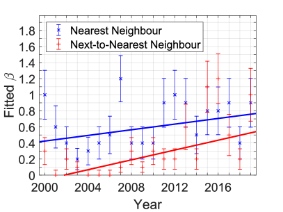
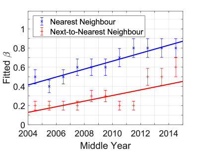
Figure 4. The effects of different group sizes. Plotted is a comparison of the NN and the NNN spacing of all collected nests $2000\!-\!2019$ with a Kolmogorov fit for the effective parameter $\beta$ of the spacing distribution, obtained from a 2D Coulomb gas (A.3) in the same way as in Figure 3, but with different numbers of years per group.
Left: No grouping, that is, each year is fitted on its own. The fluctuations that arise without grouping the years become apparent.
Right: Groups of 10 years. While the fluctuations are dampened, so is the change in $\beta$ for next-to-nearest neighbour spacing for later years. Parts of the temporal structure is lost in this way. For this reason, we choose 5 years per group as a compromise.

We therefore employ a method called bootstrapping. We generate a number of Coulomb gas realisations with a true $\beta=\beta_{0}$ and make overlapping groups of 5 realisations the same way as we do with the moving average of the nests. By fitting the $\beta$ of these realisations, we can estimate the error of the fitting method. The errors given in Figure 3 are the standard deviations of the fitted $\beta$ for the corresponding $\beta_{0}$. Because we group the realisations, we also have some information about the cross-correlation between the years. We extract this information by an average over groups of distance $k$ between the midpoint for a given $\beta_{0}$ and use $V^{\beta_{0}}_{k}$ to denote the correlation found here. We do not represent the nests completely with this method, because we only group realisations of the same $\beta_{0}$, but going into the individual $\beta_{0}$ of each year would defeat the purpose of grouping. Instead, to compare two groups with different $\beta_{0}$ and $\beta_{1}$, we use the heuristic combination

(C.2) $$V^{\beta_{0},\beta_{1}}_{k}\;=\;\sqrt{\frac{\left(V^{\beta_{0}}_{k}\right)^{2}+\left(V^{\beta_{1}}_{k}\right)^{2}}{2}}\ .$$

Here, the sum of squares reflects the structure of the least-squares error, and the 2 in the denominator ensures that $V^{\beta_{0},\beta_{0}}_{k}=V^{\beta_{0}}_{k}$. From here, we may construct the full covariance matrix of the grouped years in the left panel of Figure 3. The off-diagonal elements turn out to be small compared to the diagonal elements, so the diagonal part illustrated as error bars in Figure 3 gives a reasonable idea about the uncertainty, but should not be taken as a quantitative statement. The off-diagonal elements are, however, still included in the linear fit.

How many years are included in each group of course influences the results. We have chosen groups of $5$, because this is a compromise where fluctuations are relatively small, but the temporal structure still is visible. See Figure 4 for the effect of different choices of group size.

References

- [1] Abul-Magd, A. Y. (2006). Modelling gap-size distributions of parked cars using random-matrix theory, Physica A 368, 536–540 [arXiv:physics/0510136].
- [2] Akemann, G., Kieburg, M., Mielke, A. and Prosen, T. (2019). Universal signature from integrability to chaos in dissipative open quantum systems. Phys. Rev. Lett. 123, 254101:1–6 [arXiv:1910.03520].
- [3] Akemann, G., Phillips, M. J. and Shifrin, L. (2009). Gap probabilities in non-Hermitian random matrix theory. J. Math. Phys. 50, 063504:1–32 [arXiv:0901.0897].
- [4] Ameur, Y., Hedenmalm, H. and Makarov, N. (2011). Fluctuations of eigenvalues of random normal matrices. Duke Math. J. 159, 31–81 [arXiv:0807.0375].
-
[5]
Baake, M. and Kösters, H. (2011).
Random point sets and their diffraction.
Philos. Mag. 91, 2671–2679.
[arXiv:1007.3084]. - [6] Barlow, R. J. (1993). Statistics: A Guide to the Use of Statistical Methods in the Physical Sciences. Wiley, Chichester.
- [7] Borodin, A. and Sinclair, C. D. (2009). The Ginibre ensemble of real random matrices and its scaling limits. Commun. Math. Phys. 291, 177–224 [arXiv:0805.2986].
- [8] Chafaï, D. and Ferré, G. (2019). Simulating Coulomb gases and log-gases with hybrid Monte Carlo algorithms. J. Stat. Phys. 174, 692–714 [arXiv:1806.05985].
- [9] Chakarov, N., Boerner, M. and Krüger, O. (2008). Fitness in common buzzards at the cross–point of opposite melanin-parasite interactions. Funct. Ecol. 22, 1062–1069.
- [10] del Hoyo, J., Elliott, A. and Sargatal, J. (1994). Handbook of the Birds of the World. Vol. 2: New World Vultures to Guineafowl. Lynx Edicions, Barcelona.
- [11] De Roos, A. M. and Persson, L. (2002). Size-dependent life-history traits promote catastrophic collapses of top predators. Proc. Nat. Acad. Sci. USA (PNAS) 99, 12907–12912.
- [12] Dyson, F. J. (1962). Statistical theory of the energy levels of complex systems. J. Math. Phys. 3, 140–156.
- [13] Forrester, P. J. (2010). Log-Gases and Random Matrices. Princeton University Press, Princeton.
- [14] Gangoso, L., Agudo, R., Anadón, J. D., de la Riva, M., Suleyman, A. S., Porter, R. and Donázar, J. A. (2013). Reinventing mutualism between humans and wild fauna: insights from vultures as ecosystem services providers. Conserv. Lett. 6, 172–179.
- [15] Ginibre, J. (1965). Statistical ensembles of complex, quaternion, and real matrices. J. Math. Phys. 6, 440–449.
- [16] Grobe, R., Haake, F. and Sommers, H.-J. (1988). Quantum distinction of regular and chaotic dissipative motion. Phys. Rev. Lett. 61, 1899–1902.
- [17] Guhr, T., Müller-Groeling, A. and Weidenmüller, H. A. (1998). Random-matrix theories in quantum physics: common concepts. Phys. Rep. 299, 189–425 [arXiv:cond-mat/9707301].
- [18] Hastings, W. K. (1970). Monte Carlo sampling methods using Markov chains and their applications. Biometrika 57, 97–109.
- [19] Karr, A. F. (1991). Point Processes and their Statistical Inference. 2nd ed., Marcel Dekker, New York.
- [20] Krbálek, M. and Šeba, P. (2000). The statistical properties of the city transport in Cuernavaca (Mexico) and random matrix ensembles. J. Phys. A: Math. Gen. 33, L229–L234 [arXiv:nlin/0001015].
- [21] Krüger, O., Chakarov, N., Nielsen, J. T., Looft, V., Grünkorn, T., Struwe-Juhl, B. and Møller, A. P. (2012). Population regulation by habitat heterogeneity or individual adjustment? J. Anim. Ecol. 81, 330–340.
- [22] Krüger, O. and Lindström, J. (2001). Habitat heterogeneity affects population growth in Goshawk Accipiter gentilis. J. Anim. Ecol. 70, 173–181.
- [23] Krüger, O. and Radford, A. N. (2008). Doomed to die? Predicting extinction risk in the true hawks Accipitridae. Anim. Cons. 11, 83–91.
- [24] Lack, D. (1954). The natural regulation of animal numbers. Clarendon Press, Oxford.
- [25] Lavancier, F., Møller, J. and Rubak, E. (2015). Determinantal point process models and statistical inference. J. Royal Stat. Soc. B 77, 853–877 [arXiv:1205.4818].
- [26] Le Caër, G. (1990). Do Swedish pines diagonalise complex random matrices? Internal Report, LSG2M (Nancy, 1990), unpublished.
- [27] Le Caër, G. and Delannay, R. (1993). The administrative divisions of mainland France as 2D random cellular structures. J. Phys. I (France) 3, 1777–1800.
- [28] Markum, H., Pullirsch, R. and Wettig, T. (1999). Non-Hermitian random matrix theory and lattice QCD with chemical potential. Phys. Rev. Lett. 83, 484–487 [arXiv:hep-lat/9906020].
- [29] Müller, A. K., Chakarov, N., Heseker, H. and Krüger, O. (2016). Intraguild predation leads to cascading effects on habitat choice, behaviour and reproductive performance. J. Anim. Ecol. 85, 774–784.
- [30] Newton, I. (1979). Population Ecology of Raptors. Poyser, London.
- [31] O’Bryan, C. J., Holden, M. H. and Watson, J. E. (2019). The mesoscavenger release hypothesis and implications for ecosystem and human well-being. Ecol. Lett. 22, 1340–1348.
- [32] Rawal, S. and Rodgers, G. J. (2004). Modelling the gap size distribution of parked cars. Physica A 346, 621–630.
-
[33]
Sá, L., Ribeiro, P. and Prosen, T. (2019).
Complex spacing ratios: a signature of dissipative quantum chaos.
Preprint arXiv:1910.12784. -
[34]
Šeba, P. (2009).
Parking and the visual perception of space.
J. Stat. Mech.: Theory Exp. 2009, L10002:1–7
[arXiv:0907.1914]. - [35] Sergio, F., Newton, I. and Marchesi, L. (2005). Conservation: top predators and biodiversity. Nature 436, 192.
- [36] Serfaty, S. (2019). Microscopic description of Log and Coulomb gases. In Random Matrices, Borodin, A., Corwin, I. and Guionnet, A. (eds.), AMS, Providence, RI, 341–387 [arXiv:1709.04089].
- [37] Sibly, R. M., Barker, D., Denham, M. C., Hone, J. and Pagel, M. (2005). On the regulation of populations of mammals, birds, fish, and insects. Science 309, 607–610.
- [38] Tao, T. and Vu, V. (2015). Random matrices: universality of local spectral statistics of non-Hermitian matrices. Ann. Probab. 43, 782–874 [arXiv:1206.1893].
- [39] Wishart, J. (1928). The generalised product moment distribution in samples from a normal multivariate population. Biometrika 20A, 32–52.