Reliability and efficiency of DWR-type a posteriori error estimates with smart sensitivity weight recovering

Abstract

We derive efficient and reliable goal-oriented error estimations, and devise adaptive mesh procedures for the finite element method that are based on the localization of a posteriori estimates. In our previous work [SIAM J. Sci. Comput., 42(1), A371–A394, 2020], we showed efficiency and reliability for error estimators based on enriched finite element spaces. However, the solution of problems on a enriched finite element space is expensive. In the literature, it is well known that one can use some higher-order interpolation to overcome this bottleneck. Using a saturation assumption, we extend the proofs of efficiency and reliability to such higher-order interpolations. The results can be used to create a new family of algorithms, where one of them is tested on three numerical examples (Poisson problem, p-Laplace equation, Navier-Stokes benschmark), and is compared to our previous algorithm.

1 Introduction

Goal-oriented error estimation using adjoints was established in [8, 9], and is a current research topic as attested in many studies. Recent developments include Fractional-Step-$\theta$ Galerkin formulations [39], a partition-of-unity variational localization [44], phase-field fracture problems [50], surrogate constructions for stochastic inversion [36], general adaptive multiscale modeling [41], model adaptivity in multiscale problems [34], multigoal-oriented error estimation with balancing discretization and iteration errors [20], nonstationary, nonlinear fluid-structure interaction [25], realizations on polygonal meshes using boundary-element based finite elements [49], realizations using the finite cell method [46], error estimation for sea ice simulations [37], discretization error estimation in computer assisted surgery [18], and a unifying framework with inexact solvers covering discontinuous Galerkin and finite volume approaches [35]. An open-source framework for linear, time-dependent, goal-oriented error estimation was published in [32]. Abstract convergence results of goal-oriented techniques were studied in [30] and [26]. A worst-case multigoal-oriented error estimation was carried out in [47]. Recently, using a saturation assumption, e.g., [17, 13, 26, 5], two-side error estimates, namely efficiency and robustness of the adjoint-based error estimator, could be shown [21].

In most realizations, an adjoint problem is used in order to determine sensitivities that enter the error in a single target functional [9, 42] or multiple quantities of interest [28, 22, 20]. In [42, 20], balancing of discretization and nonlinear iteration errors for single and multiple goal functionals was considered, respectively. However, for nonlinear problems, sensitivity weights in the primal and adjoint variable are necessary. These weights must be of higher-order. Otherwise they yield zero sensitivities, and, therefore, the entire error estimator vanishes. The most straightforward way is to use higher-order finite element spaces [9]. A computationally cheaper approach based on low-order finite elements and then a patch-wise higher-order interpolation was suggested as well in the early stages [9] and combined in an elegant way to a weak localization in [12]. Rigorous proofs of effectivity measured in mesh-dependent norms, in which the true error and the estimator satisfy a common upper bound, were established in [44]. Therein, saturation assumptions where not required, but the results of effectivity are weaker than in our recent work [21]. More specifically, in [21], the adjoint problem is solved in a higher-order space and then interpolated into the low-order space for calculating the interpolation error. For this procedure, two-side error estimates are proven, while using the previously mentioned saturation assumption.

The objective of this paper is now the other way around, namely efficiency proofs (under saturation assumptions) for interpolations from low-order finite element spaces into higher-order spaces, which are not present in the literature to date. We establish results when both the primal and adjoint problems are computed only in low-order finite element spaces. To this end, two additional error terms will be introduced. The resulting error estimator holds for nonlinear PDEs and nonlinear goal functionals, and accounts for the discretization error, nonlinear iteration error and the interpolation error. These derivations lead to a novel adaptive algorithm that works at low computational cost in goal-oriented frameworks. Our theoretical and algorithmic developments are then substantiated with the help of several numerical tests. It is known that the saturation assumption may be violated for transport or convection-dominated problems. We provide one numerical test in which this is the case. Furthermore, linear and nonlinear problem configurations are considered to cover most relevant classes of stationary, nonlinear settings.

The outline of this paper is as follows: In Section 2, an abstract setting for the DWR method is introduced. Then, in Section 3, the DWR approach with general approximations is stated. A discussion of all terms of the newly proposed error estimator is provided in Section 4. Based on these findings, an adaptive algorithm is designed in Section 5. Several numerical tests with linear PDEs and linear goal functionals, nonlinear settings, and a stationary Navier-Stokes configuration are carried out in Section 6. We summarize our results in Section 7.

2 An abstract setting and the dual weighted resiudal method

In this section, we briefly introduce the notation and the settings that we consider in this work. These are similar to our previous studies [20, 21].

2.1 An abstract setting

Let $U$ and $V$ be reflexive Banach spaces, and let $\mathcal{A}:U\mapsto V^{*}$ be a nonlinear mapping, where $V^{*}$ denotes the dual space of the Banach space $V$. We consider the problem: Find $u\in U$ such that

$$\mathcal{A}(u)=0\qquad\text{ in }V^{*}.$$ (1)

This problem will be refereed as the primal problem. As mapping we have in mind some (possibly) nonlinear partial differential operator. Furthermore, we consider finite dimensional subspaces of $U_{h}\subset U$ and $V_{h}\subset V$. In this work, $U_{h}$ and $V_{h}$ are finite element spaces . This leads to the following finite dimensional problem: Find $u_{h}\in U_{h}$ such that

$$\mathcal{A}(u_{h})=0\qquad\text{ in }V_{h}^{*}.$$ (2)

We assume that the problem (1) as well as the finite dimensional problem (2) are solvable. Further conditions will be imposed when needed. However, we do not aim for the solution $u$. The goal is to obtain one characteristic quantity (quantity of interest) $J(u)\in\mathbb{R}$, i.e., a functional evaluation, evaluated at the solution $u\in U$ , where $J:U\mapsto\mathbb{R}$.

2.2 The dual weighted residual method

In this section, we briefly review the Dual Weighted Residual (DWR) method for nonlinear problems. This work was extended to balance the discretization and iteration errors in [42, 43, 38].

This paper forms together with our previous works [20, 21] the basis of the current study. Since the DWR method is an adjoint based method, we consider the adjoint problem: Find $z\in V$ such that

$$\left(\mathcal{A}^{\prime}(u)\right)^{*}(z)=J^{\prime}(u)\qquad\text{ in }U^{*},$$ (3)

where $\mathcal{A}^{\prime}(u)$ and $J^{\prime}(u)$ are the Fréchet-derivatives of the nonlinear operator and functional, respectively, evaluated at the solution of the primal problem $u$. In the following sections, we require a finite dimensional version of (3) that reads as follows: Find $z_{h}\in V_{h}$ such that

$$\left(\mathcal{A}^{\prime}(u_{h})\right)^{*}(z_{h})=J^{\prime}(u_{h})\qquad\text{ in }U_{h}^{*}.$$

Similarly to the findings in [42, 9, 43, 21], we obtain an error representation in the following theorem:

Theorem 2.1.

Let us assume that $\mathcal{A}\in\mathcal{C}^{3}(U,V)$ and $J\in\mathcal{C}^{3}(U,\mathbb{R})$. If $u$ solves (1) and $z$ solves (3) for $u\in U$, then the error representation

$$\begin{split}J(u)-J(\tilde{u})&=\frac{1}{2}\rho(\tilde{u})(z-\tilde{z})+\frac{1}{2}\rho^{*}(\tilde{u},\tilde{z})(u-\tilde{u})-\rho(\tilde{u})(\tilde{z})+\mathcal{R}^{(3)},\end{split}$$

holds true for arbitrary fixed $\tilde{u}\in U$ and $\tilde{z}\in V$, where $\rho(\tilde{u})(\cdot):=-\mathcal{A}(\tilde{u})(\cdot)$, $\rho^{*}(\tilde{u},\tilde{z})(\cdot):=J^{\prime}(u)-\mathcal{A}^{\prime}(\tilde{u})(\cdot,\tilde{z})$, and the remainder term

$$\begin{split}\mathcal{R}^{(3)}:=\frac{1}{2}\int_{0}^{1}\big{[}J^{\prime\prime\prime}(\tilde{u}+se)(e,e,e)-\mathcal{A}^{\prime\prime\prime}(\tilde{u}+se)(e,e,e,\tilde{z}+se^{*})-3\mathcal{A}^{\prime\prime}(\tilde{u}+se)(e,e,e)\big{]}s(s-1)\,ds,\end{split}$$ (4)

with $e=u-\tilde{u}$ and $e^{*}=z-\tilde{z}$.

Proof.

The proof is given in [20]. ∎

For the arbitrary elements $\tilde{u}$ and $\tilde{z}$, we think of approximations to the discrete solutions $u_{h}$ and $z_{h}$. The resulting error estimator reads as

$$\eta=\frac{1}{2}\rho(\tilde{u})(z-\tilde{z})+\frac{1}{2}\rho^{*}(\tilde{u},\tilde{z})(u-\tilde{u})+\rho(\tilde{u})(\tilde{z})+\mathcal{R}^{(3)}.$$

This error estimator is exact, but it still depends on the unknown solutions $u$ and $z$. Therefore, it is not computable. To obtain a computable error estimator, one can replace the exact solutions $u$ and $z$ by an approximate solution on enriched finite dimensional spaces $U_{h}^{(2)}$ and $V_{h}^{(2)}$. This was already discussed in [9, 4]. Some efficiency and reliability results for this replacement are discussed in [21]. Other replacements will be covered by the theory in this work. This includes (patch-wise) reconstructions as suggested in [9, 4, 12] .

3 DWR error estimation using general approximations

In this key section, the DWR estimator is augmented to deal with general approximations such as interpolations. The latter allow for a very cost-efficient realization of the DWR estimator for both linear and nonlinear problems. These improvements are significant. However, it turns out that the governing proofs have the same structure as in Section 3 in our previous work [21]. Therein, it was assumed that the solutions on enriched spaces are known.

In the current work, we consider that we just have some arbitrary approximations in the enriched spaces. Examples how this is done are by inaccurate or accurate solves on the enriched space or (patch-wise) higher-order interpolation operators [9, 4]. We show efficiency and reliability for an alternate form of the error estimator using some saturation assumption for the goal functional on two different kind of approximations. In other words, this means that the approximations in the enriched spaces deliver a more accurate result in the quantity of interest than the approximation of $u_{h}$.

3.1 Results on discrete spaces

Let $\tilde{u}_{h}^{(2)}\in U_{h}^{(2)}$ be some arbitrary but fixed approximation of the primal problem: Find ${u}_{h}^{(2)}\in U_{h}^{(2)}$ such that $\mathcal{A}({u}_{h}^{(2)})=0$ in $(V_{h}^{(2)})^{*}$, and $\tilde{z}_{h}^{(2)}\in V_{h}^{(2)}$ be an approximation to the discretized adjoint problem : Find ${z}_{h}^{(2)}\in V_{h}^{(2)}$ $(\mathcal{A^{\prime}}({u}_{h}^{(2)}))^{*}({z}_{h}^{(2)})=J^{\prime}({u}_{h}^{(2)})$ in $(U_{h}^{(2)})^{*}.$

Theorem 3.1.

Let us assume that $\mathcal{A}\in\mathcal{C}^{3}(U,V)$ and $J\in\mathcal{C}^{3}(U,\mathbb{R})$, and let $\tilde{u}\in U$ and $\tilde{z}\in V$ be arbitrary but fixed. If $\tilde{u}_{h}^{(2)}\in U_{h}^{(2)}$ and $\tilde{z}_{h}^{(2)}\in V_{h}^{(2)}$ are some approximations of $u$ and $z$, then the error representation

$$\begin{split}J(\tilde{u}_{h}^{(2)})-J(\tilde{u})&=\frac{1}{2}\rho(\tilde{u})(\tilde{z}_{h}^{(2)}-\tilde{z})+\frac{1}{2}\rho^{*}(\tilde{u},\tilde{z})(\tilde{u}_{h}^{(2)}-\tilde{u})-\rho(\tilde{u})(\tilde{z})\\ &-\rho(\tilde{u}_{h}^{(2)})(\frac{\tilde{z}_{h}^{(2)}+\tilde{z}}{2})+\frac{1}{2}\rho^{*}(\tilde{u}_{h}^{(2)},\tilde{z}_{h}^{(2)})(\tilde{u}_{h}^{(2)}-\tilde{u})+\tilde{\mathcal{R}}^{(3)(2)}\end{split}$$

holds. In this error representation, the new terms in comparison to [21] are

$$\rho(\tilde{u}_{h}^{(2)})(\frac{\tilde{z}_{h}^{(2)}+\tilde{z}}{2})\quad\text{and}\quad\frac{1}{2}\rho^{*}(\tilde{u}_{h}^{(2)},\tilde{z}_{h}^{(2)})(\tilde{u}_{h}^{(2)}-\tilde{u}).$$

Furthermore, we have $\rho(\tilde{u})(\cdot):=-\mathcal{A}(\tilde{u})(\cdot)$ and $\rho^{*}(\tilde{u},\tilde{z})(\cdot):=J^{\prime}(u)-\mathcal{A}^{\prime}(\tilde{u})(\cdot,\tilde{z})$ as usual. Finally, the remainder term is given by

$$\begin{split}\tilde{\mathcal{R}}^{(3)(2)}:=\frac{1}{2}\int_{0}^{1}[J^{\prime\prime\prime}(\tilde{u}+se)(e,e,e)-\mathcal{A}^{\prime\prime\prime}(\tilde{u}+se)(e,e,e,\tilde{z}+se^{*})-3\mathcal{A}^{\prime\prime}(\tilde{u}+se)(e,e,e)]s(s-1)\,ds,\end{split}$$

with $e=\tilde{u}_{h}^{(2)}-\tilde{u}$ and $e^{*}=\tilde{z}_{h}^{(2)}-\tilde{z}$.

Proof.

The proof is an extension of [42]. First we define a general approximation $x:=(\tilde{u}_{h}^{(2)},\tilde{z}_{h}^{(2)})\in X:=U\times V$ and $\tilde{x}:=(\tilde{u},\tilde{z})\in X$. Assuming that $\mathcal{A}\in\mathcal{C}^{3}(U,V)$ and $J\in\mathcal{C}^{3}(U,\mathbb{R})$, we know that the Lagrange functional, which is given by

$$\mathcal{L}(\hat{x}):=J(\hat{u})-\mathcal{A}(\hat{u})(\hat{z})\quad\forall(\hat{u},\hat{z})=:\hat{x}\in X,$$

belongs to $\mathcal{C}^{3}(X,\mathbb{R})$. This allows us to derive the following identity

$$\mathcal{L}(x)-\mathcal{L}(\tilde{x})=\int_{0}^{1}\mathcal{L}^{\prime}(\tilde{x}+s(x-\tilde{x}))(x-\tilde{x})\,ds.$$

Using the trapezoidal rule

$$\int_{0}^{1}f(s)\,ds=\frac{1}{2}(f(0)+f(1))+\frac{1}{2}\int_{0}^{1}f^{\prime\prime}(s)s(s-1)\,ds,$$

with $f(s):=\mathcal{L}^{\prime}(\tilde{x}+s(x-\tilde{x}))(x-\tilde{x})$, cf. [42], we obtain

$$\mathcal{L}(x)-\mathcal{L}(\tilde{x})= \frac{1}{2}(\mathcal{L}^{\prime}(x)(x-\tilde{x})+\mathcal{L}^{\prime}(\tilde{x})(x-\tilde{x}))+\mathcal{R}^{(3)}.$$

From the definition of $\mathcal{L}$, we observe that

$$J(\tilde{u}_{h}^{(2)})-J(\tilde{u})= \mathcal{L}(x)-\mathcal{L}(\tilde{x})+{A(\tilde{u}_{h}^{(2)})(\tilde{z}_{h}^{(2)})}-A(\tilde{u})(\tilde{z})$$

$$= \frac{1}{2}(\mathcal{L}^{\prime}(x)(x-\tilde{x})+\mathcal{L}^{\prime}(\tilde{x})(x-\tilde{x}))+A(\tilde{u}_{h}^{(2)})(\tilde{z}_{h}^{(2)})-A(\tilde{u})(\tilde{z})+\tilde{\mathcal{R}}^{(3)(2)}.$$

It holds

$$\mathcal{L}^{\prime}(x)(x-\tilde{x})+\mathcal{L}^{\prime}(\tilde{x})(x-\tilde{x})= \underbrace{J^{\prime}(\tilde{u}_{h}^{(2)})(e)-\mathcal{A}^{\prime}(\tilde{u}_{h}^{(2)})(e,\tilde{z}_{h}^{(2)})}_{=\rho^{*}(\tilde{u}_{h}^{(2)},\tilde{z}_{h}^{(2)})(\tilde{u}_{h}^{(2)}-\tilde{u})}-{A(\tilde{u}_{h}^{(2)})(e^{*})}$$

$$+ \underbrace{J^{\prime}(\tilde{u})(e)-\mathcal{A}^{\prime}(\tilde{u})(e,\tilde{z})}_{=\rho^{*}(\tilde{u},\tilde{z})(\tilde{u}_{h}^{(2)}-\tilde{u})}-\underbrace{A(\tilde{u})(e^{*})}_{=\rho(\tilde{u})(\tilde{z}_{h}^{(2)}-\tilde{z})}.$$

Further manipulations and rewriting, together with

$$-\frac{1}{2}A(\tilde{u}_{h}^{(2)})(e^{*})+{A(\tilde{u}_{h}^{(2)})(\tilde{z}_{h}^{(2)})}=A(\tilde{u}_{h}^{(2)})(-\frac{1}{2}\tilde{z}_{h}^{(2)}+\frac{1}{2}\tilde{z}+\tilde{z}_{h}^{(2)}))={A(\tilde{u}_{h}^{(2)})(\frac{\tilde{z}_{h}^{(2)}+\tilde{z}}{2})},$$

yield

$$J(\tilde{u}_{h}^{(2)})-J(\tilde{u})=\frac{1}{2}\big{(}\rho^{*}(\tilde{u}_{h}^{(2)},\tilde{z}_{h}^{(2)})(\tilde{u}_{h}^{(2)}-\tilde{u})-A(\tilde{u}_{h}^{(2)})(e^{*})+\rho(\tilde{u})(\tilde{z}_{h}^{(2)}-\tilde{z})+\rho^{*}(\tilde{u},\tilde{z})(\tilde{u}_{h}^{(2)}-\tilde{u})\big{)}$$

$$+{A(\tilde{u}_{h}^{(2)})(\tilde{z}_{h}^{(2)})})-A(\tilde{u})(\tilde{z})+\tilde{\mathcal{R}}^{(3)(2)}$$

$$=\frac{1}{2}\big{(}{{\rho^{*}(\tilde{u}_{h}^{(2)},\tilde{z}_{h}^{(2)})(\tilde{u}_{h}^{(2)}-\tilde{u})}+\rho(\tilde{u})(\tilde{z}_{h}^{(2)}-\tilde{z})+\rho^{*}(\tilde{u},\tilde{z})(\tilde{u}_{h}^{(2)}-\tilde{u})}\big{)}$$

$$+\underbrace{{A(\tilde{u}_{h}^{(2)})(\frac{\tilde{z}_{h}^{(2)}+\tilde{z}}{2})})}_{=-\rho(\tilde{u}_{h}^{(2)})(\frac{\tilde{z}_{h}^{(2)}+\tilde{z}}{2})}+A(\tilde{u})(\tilde{z})+\tilde{\mathcal{R}}^{(3)(2)}.$$

These last statements prove the assertion. ∎

Remark 3.2.

If we use the solutions of the adjoint and the primal problem on the enriched spaces for computing $\tilde{z}_{h}^{(2)}$ and $\tilde{u}_{h}^{(2)}$, respectively, then

$$\rho(\tilde{u}_{h}^{(2)})(\frac{\tilde{z}_{h}^{(2)}+\tilde{z}}{2})=0\quad\mbox{ and }\quad\frac{1}{2}\rho^{*}(\tilde{u}_{h}^{(2)},\tilde{z}_{h}^{(2)})(\tilde{u}_{h}^{(2)}-\tilde{u})=0.$$

Remark 3.3.

A practial choice for $\tilde{z}_{h}^{(2)}$ and $\tilde{u}_{h}^{(2)}$ is, that we can construct higher-order interpolations from $\tilde{z}_{h}$ and $\tilde{u}_{h}$. This allows to compute all subproblems with low-order finite elements and the error estimator can be constructed in a cheap way. Under a saturation assumption we prove some results for this well known interpolation techniques.

Theorem 3.1 motivates the following choice of the error estimator.

$$\tilde{\eta}^{(2)}:=\frac{1}{2}\rho(\tilde{u})(\tilde{z}_{h}^{(2)}-\tilde{z})+\frac{1}{2}\rho^{*}(\tilde{u},\tilde{z})(\tilde{u}_{h}^{(2)}-\tilde{u})-\rho(\tilde{u})(\tilde{z})-\rho(\tilde{u}_{h}^{(2)})(\frac{\tilde{z}_{h}^{(2)}+\tilde{z}}{2})+\\ \frac{1}{2}\rho^{*}(\tilde{u}_{h}^{(2)},\tilde{z}_{h}^{(2)})(\tilde{u}_{h}^{(2)}-\tilde{u})+\tilde{\mathcal{R}}^{(3)(2)}.$$ (5)

3.2 Two-sided estimates for DWR using a saturation assumption

In the upcoming lemma, we derive two-sided bounds (efficiency and reliablity) for the error estimator $\tilde{\eta}^{(2)}$ defined by (5).

Lemma 3.4.

If the assumptions of Theorem 2.1 are fulfilled, then the computable error estimator $\tilde{\eta}^{(2)}$ can be bounded from below and above as follows:

$$|J(u)-J(\tilde{u})|-|J(u)-J(\tilde{u}_{h}^{(2)})|\leq|\tilde{\eta}^{(2)}|\leq|J(u)-J(\tilde{u})|+|J(u)-J(\tilde{u}_{h}^{(2)})|.$$

Proof.

We proof the bounds in the same way as in [21]. We know that $|\eta|=|\tilde{\eta}^{(2)}-(\tilde{\eta}^{(2)}-\eta)|$, and therefore, we can conclude that

$$|\eta|-|\eta-\tilde{\eta}^{(2)}|\leq|\tilde{\eta}^{(2)}|\leq|\eta|+|\eta-\tilde{\eta}^{(2)}|.$$

The statement of the lemma follows with the identities, $\eta-\tilde{\eta}^{(2)}=J(u)-J(\tilde{u})-J(\tilde{u}_{h}^{(2)})+J(\tilde{u})=J(u)-J(\tilde{u}_{h}^{(2)})$ and $\eta=J(u)-J(\tilde{u})$. ∎

In the sequel, we impose a saturation assumption, which is a common assumption in hierarchical based error estimation [7, 10, 6, 48]. Even if the solutions of the primal and adjoint problem in the enriched spaces are used, the saturation assumption may be violated as shown in [10, 21].

However, for particular problems, quantities of interest and refinements, it is possible to show the saturation assumption [17, 2, 1, 27, 5, 13, 23, 16]. It heavily depends on the quantity of interest, the finite dimensional spaces and the problem. We impose the following assumption, which is a slight generalization to [21].

Assumption 1 (Saturation assumption for the goal functional).

Let $\tilde{u}_{h}^{(2)}$ be an arbitrary, but fixed approximation in $U_{h}^{(2)}$, and let $\tilde{u}$ be some approximation in $U_{h}$. Then we assume that

$$|J(u)-J(\tilde{u}_{h}^{(2)})|<b_{h}|J(u)-J(\tilde{u})|$$

for some $b_{h}<b_{0}$ and some fixed $b_{0}\in(0,1)$.

Remark 3.5.

For gradient based functionals like the flux, one can use recovering techniques to reconstruct the gradient as in [33]. Here, under certain conditions, the saturation assumption can be shown.

Remark 3.6.

If $J(u)$ is just a point evaluation and the given point is a node in the mesh, then $|J(u)-J(\tilde{u}_{h}^{(2)})|=|J(u)-J(\tilde{u})|$ in the case of higher-order interpolation as used in [9, 42, 4]. Therefore, the saturation assumption is never fulfilled. If the given point is not on the grid, then $|J(u)-J(\tilde{u}_{h}^{(2)})|$ converges to $|J(u)-J(\tilde{u})|$ provided that the mesh is locally refine around the evaluation point.

Theorem 3.7.

Let the Assumption 1 be fulfilled. Then the computable error estimator $\tilde{\eta}^{(2)}$ is efficient and reliable, i.e.

$$\underline{c}_{h}|\tilde{\eta}^{(2)}|\leq|J(u)-J(\tilde{u})|\leq\overline{c}_{h}|\tilde{\eta}^{(2)}|\quad\mbox{and}\quad\underline{c}|\tilde{\eta}^{(2)}|\leq|J(u)-J(\tilde{u})|\leq\overline{c}|\tilde{\eta}^{(2)}|,$$

where $\underline{c}_{h}:=1/(1+b_{h})$, $\overline{c}_{h}:=1/(1-b_{h})$, $\underline{c}:=1/(1+b_{0})$, and $\overline{c}:=1/(1-b_{0})$.

Proof.

The proof follows from the estimates given in the proof of Lemma 3.4 and simple computations. We follow the same steps as in the proof of Theorem 3.3 in [21]. ∎

Following [42, 21], we consider the practical discretization error estimator

$$\tilde{\eta}_{h}^{(2)}:=\frac{1}{2}\rho(\tilde{u})(\tilde{z}_{h}^{(2)}-\tilde{z})+\frac{1}{2}\rho^{*}(\tilde{u},\tilde{z})(\tilde{u}_{h}^{(2)}-\tilde{u}),$$ (6)

that corresponds to the theoretical discretization error estimator

$$\eta_{h}:=\frac{1}{2}\rho(\tilde{u})(z-\tilde{z})+\frac{1}{2}\rho^{*}(\tilde{u},\tilde{z})(u-\tilde{u}).$$

Lemma 3.8.

Let $\eta_{h}$ and $\tilde{\eta}_{h}^{(2)}$ be as defined above, and let $\tilde{u}\in U$ and $\tilde{z}\in V$ be arbitrary but fixed. Furthermore, we assume that $\mathcal{A}\in\mathcal{C}^{3}(U,V)$ and $J\in\mathcal{C}^{3}(U,\mathbb{R})$. If $\tilde{u}_{h}^{(2)}\in U_{h}^{(2)}$ and $\tilde{z}_{h}^{(2)}\in V_{h}^{(2)}$ are some approximations to $u\in U$ and $z\in V$, respectively, then, for the approximations $\tilde{u}_{h}^{(2)}$ and $\tilde{z}_{h}^{(2)}$ from the enriched spaces $U_{h}^{(2)}$ and $V_{h}^{(2)}$, the following estimates

$$\begin{split}|J(u)-J(\tilde{u}_{h}^{(2)})|-|\mathcal{R}^{(3)}-\tilde{\mathcal{R}}^{(3)(2)}|-|\tilde{\eta}_{\tilde{z}_{h}^{(2)}}|-|\tilde{\eta}_{\tilde{u}_{h}^{(2)}}|\leq|\eta_{h}-\tilde{\eta}_{h}^{(2)}|,\\ |\eta_{h}-\tilde{\eta}_{h}^{(2)}|\leq|J(u)-J(\tilde{u}_{h}^{(2)})|+|\mathcal{R}^{(3)}-\tilde{\mathcal{R}}^{(3)(2)}|+|\tilde{\eta}_{\tilde{z}_{h}^{(2)}}|+|\tilde{\eta}_{\tilde{u}_{h}^{(2)}}|,\end{split}$$ (7)

and

$$|J(u)-J(\tilde{u})|-|\rho(\tilde{u})(\tilde{z})|-|\mathcal{R}^{(3)}|\leq|\eta_{h}|\leq|J(u)-J(\tilde{u})|+|\rho(\tilde{u})(\tilde{z})|+|\mathcal{R}^{(3)}|$$ (8)

hold. Here, $\mathcal{R}^{(3)}$ is defined in (4), $\tilde{\mathcal{R}}^{(3)(2)}$ is from Theorem 3.1, and we have

$$\tilde{\eta}_{\tilde{u}_{h}^{(2)}}:=-\rho(\tilde{u}_{h}^{(2)})(\frac{\tilde{z}_{h}^{(2)}+\tilde{z}}{2}),\qquad\tilde{\eta}_{\tilde{z}_{h}^{(2)}}:=\frac{1}{2}\rho^{*}(\tilde{u}_{h}^{(2)},\tilde{z}_{h}^{(2)})(\tilde{u}_{h}^{(2)}-\tilde{u}).$$

Proof.

The inequality (8) was already proven in [21]. From Theorem 2.1 and Theorem 3.1, we get the identities

$$J(u)-J(\tilde{u})=\underbrace{\frac{1}{2}\rho(\tilde{u})(z-\tilde{z})+\frac{1}{2}\rho^{*}(\tilde{u},\tilde{z})(u-\tilde{u})}_{\eta_{h}}+\rho(\tilde{u})(\tilde{z})+\mathcal{R}^{(3)},$$

and

$$J(\tilde{u}_{h}^{(2)})-J(\tilde{u})=\underbrace{\frac{1}{2}\rho(\tilde{u})(\tilde{z}_{h}^{(2)}-\tilde{z})+\frac{1}{2}\rho^{*}(\tilde{u},\tilde{z})(\tilde{u}_{h}^{(2)}-\tilde{u})}_{\tilde{\eta}_{h}^{(2)}}+\tilde{\eta}_{\tilde{u}_{h}^{(2)}}+\tilde{\eta}_{\tilde{z}_{h}^{(2)}}+\rho(\tilde{u})(\tilde{z})+\tilde{\mathcal{R}}^{(3)(2)}.$$

If we substract the equations from above, then we obtain

$$J(u)-J(\tilde{u}_{h}^{(2)})=\eta_{h}-{\tilde{\eta}_{h}^{(2)}}+\mathcal{R}^{(3)}-\tilde{\mathcal{R}}^{(3)(2)}-\tilde{\eta}_{\tilde{u}_{h}^{(2)}}-\tilde{\eta}_{\tilde{z}_{h}^{(2)}}.$$

From this equality, we conclude (7) by using triangle inequality. ∎

Remark 3.9.

Indeed a refined analysis yields the inequalities

$$|J(u)-J(\tilde{u}_{h}^{(2)})|-|\mathcal{R}^{(3)}-\tilde{\mathcal{R}}^{(3)(2)}-\tilde{\eta}_{\tilde{u}_{h}^{(2)}}-\tilde{\eta}_{\tilde{z}_{h}^{(2)}}|\leq|\eta_{h}-\tilde{\eta}_{h}^{(2)}|\leq|J(u)-J(\tilde{u}_{h}^{(2)})|+|\mathcal{R}^{(3)}-\tilde{\mathcal{R}}^{(3)(2)}-\tilde{\eta}_{\tilde{u}_{h}^{(2)}}-\tilde{\eta}_{\tilde{z}_{h}^{(2)}}|.$$

Similar as in [21], we can now show the following result:

Lemma 3.10.

If the conditions of Lemma 3.8 are fulfilled, then the inequalities

$$|\tilde{\eta}_{h}^{(2)}|-\gamma(\mathcal{A},J,\tilde{u}_{h}^{(2)},\tilde{z}_{h}^{(2)},u,\tilde{u},\tilde{z})\leq|J(u)-J(\tilde{u})|\leq|\tilde{\eta}_{h}^{(2)}|+\gamma(\mathcal{A},J,\tilde{u}_{h}^{(2)},\tilde{z}_{h}^{(2)},u,\tilde{u},\tilde{z})$$

are valid, where

$$\gamma(\mathcal{A},J,\tilde{u}_{h}^{(2)},\tilde{z}_{h}^{(2)},u,\tilde{u},\tilde{z}):=|J(u)-J(\tilde{u}_{h}^{(2)})|+|\mathcal{R}^{(3)}-\tilde{\mathcal{R}}^{(3)(2)}|+|\tilde{\eta}_{\tilde{z}_{h}^{(2)}}|+|\tilde{\eta}_{\tilde{u}_{h}^{(2)}}|+|\rho(\tilde{u})(\tilde{z})|+|\mathcal{R}^{(3)}|.$$ (9)

Proof.

The proof follows the same idea as in the proof of Lemma 3.8 in [21]. ∎

3.3 Computable error estimator under a strengthend saturation assumption

Under a strengthened saturation assumption, the results from above can also be derived for the discretization error estimator $\tilde{\eta}_{h}^{(2)}$. We suppose the following:

Assumption 2 (Strengthened saturation assumption for the goal functional).

Let $\tilde{u}_{h}^{(2)}$ be an arbitrary, but fixed approximation in $U_{h}^{(2)}$, and let $\tilde{u}$ be some approximation. Then the inequality

$$\gamma(\mathcal{A},J,\tilde{u}_{h}^{(2)},\tilde{z}_{h}^{(2)},u,\tilde{u},\tilde{z})<b_{h,\gamma}|J(u)-J(\tilde{u})|,$$

holds for some $b_{h,\gamma}<b_{0,\gamma}$ with some fixed $b_{0,\gamma}\in(0,1)$, where $\gamma(\cdot)$ is defined in (9).

Remark 3.11.

Assumption 2 implies Assumption 1. However, if vice versa, Assumption 1 holds, then Assumption 2 is fulfilled up to higher-order terms ($|\mathcal{R}^{(3)}-\tilde{\mathcal{R}}^{(3)(2)}|$, $|\mathcal{R}^{(3)}|$), and by the parts $|\rho(\tilde{u})(\tilde{z})|$, $\tilde{\eta}_{\tilde{u}_{h}^{(2)}}$, $\tilde{\eta}_{\tilde{z}_{h}^{(2)}}$ which can be controlled by the accuracy of the approximations. In particular, if the approximation $\tilde{u}_{h}^{(2)}$ in the enriched space coincides with the finite element solution ${u}_{h}^{(2)}$, i.e. ${u}_{h}^{(2)}=\tilde{u}_{h}^{(2)}$, then $\tilde{\eta}_{\tilde{u}_{h}^{(2)}}=0$. If the same condition, i.e. ${z}_{h}^{(2)}=\tilde{z}_{h}^{(2)}$, is fulfilled for the adjoint problem, then $\tilde{\eta}_{\tilde{z}_{h}^{(2)}}=0.$

Theorem 3.12.

Let Assumption 2 be satisfied. Then the practical error estimator $\tilde{\eta}_{h}^{(2)}$, defined in (6), is efficient and reliable, i.e.

$$\underline{c}_{h,\gamma}|\tilde{\eta}_{h}^{(2)}|\leq|J(u)-J(\tilde{u})|\leq\overline{c}_{h,\gamma}|\tilde{\eta}_{h}^{(2)}|\quad\mbox{and}\quad\underline{c}_{\gamma}|\tilde{\eta}_{h}^{(2)}|\leq|J(u)-J(\tilde{u})|\leq\overline{c}_{\gamma}|\tilde{\eta}_{h}^{(2)}|,$$

with the positive constants $\underline{c}_{h,\gamma}:=1/(1+b_{h,\gamma})$, $\overline{c}_{h,\gamma}:=1/(1-b_{h,\gamma})$, $\underline{c}_{\gamma}:=1/(1+b_{0,\gamma})$, $\overline{c}_{\gamma}:=1/(1-b_{0,\gamma})$.

Proof.

The proof follows the same steps as in [21]. The result can be derived from Lemma 3.10 and Assumption 2. For further information, we refer to the proof in [21]. ∎

3.4 Bounds of the effectivity indices

As in [21] we derive bounds for the effectivity indices $I_{eff}$ and $I_{eff,h}$ which are defined by

$$I_{eff}:=\frac{|\tilde{\eta}^{(2)}|}{|J(u)-J(\tilde{u})|}\quad\mbox{and}\quad I_{eff,h}:=\frac{|\tilde{\eta}_{h}^{(2)}|}{|J(u)-J(\tilde{u})|},$$ (10)

respectively. The quantities $\tilde{\eta}^{(2)}$ and $\tilde{\eta}_{h}^{(2)}$ are defined as in (5) and (6). We then obtain:

Theorem 3.13 (Bounds on the effectivity index).

Let us assume that $\mathcal{A}\in\mathcal{C}^{3}(U,V)$ and $J\in\mathcal{C}^{3}(U,\mathbb{R})$, and let $\tilde{u}\in U$ and $\tilde{z}\in V$ be arbitrary, but fixed. Then the following two statements are true:

1. If Assumption 1 is fulfilled, then $I_{eff}\in[1-b_{0},1+b_{0}]$, and if additionally $b_{h}\rightarrow 0$, then $I_{eff}\rightarrow 1$.

2. If Assumption 2 is fulfilled, then $I_{eff,h}\in[1-b_{0,\gamma},1+b_{0,\gamma}]$, and if additionally $b_{h,\gamma}\rightarrow 0$, then $I_{eff,h}\rightarrow 1$.

Proof.

The bounds immediately follow from Lemma 3.4 and Assumption 1, and Lemma 3.10 and Assumption 2. ∎

Remark 3.14.

In practice, the efficiency indices

$$I_{eff,\mathcal{R}}:=\frac{|\tilde{\eta}_{h}^{(2)}-\rho(\tilde{u})(\tilde{z})+\tilde{\mathcal{R}}^{(3)(2)}|}{|J(u)-J(\tilde{u})|}$$

and $I_{eff,h}$ almost coincide.

Remark 3.15.

In this section, we omit errors coming from inexact data approximation and numerical quadrature.

4 Separation of the error estimator parts

In this section, we briefly describe the different parts of the error estimator. The error estimator, which is derived in the previous section, consists of five parts. The first three parts $\tilde{\eta}_{h}^{(2)}$, $\eta_{k}$, $\eta^{(2)}_{\mathcal{R}}$ were already discussed in [21]. We will now focus on the fourth and fifth part, which are novel. For completeness of presentations, we give a short recap about the other parts.

Proposition 4.1.

We split $\tilde{\eta}^{(2)}$ defined in (5) into the following five parts $\tilde{\eta}_{h}^{(2)}$, $\eta_{k}$, $\eta^{(2)}_{\mathcal{R}}$, $\tilde{\eta}_{\tilde{u}_{h}^{(2)}}$, and $\tilde{\eta}_{\tilde{z}_{h}^{(2)}}$:

$$\footnotesize\tilde{\eta}^{(2)}:=\underbrace{\frac{1}{2}\rho(\tilde{u})(\tilde{z}_{h}^{(2)}-\tilde{z})+\frac{1}{2}\rho^{*}(\tilde{u},\tilde{z})(\tilde{u}_{h}^{(2)}-\tilde{u})}_{:=\tilde{\eta}_{h}^{(2)}}-\underbrace{\rho(\tilde{u})(\tilde{z})}_{:=\eta_{k}}+\underbrace{\tilde{\mathcal{R}}^{(3)(2)}}_{:=\eta^{(2)}_{\mathcal{R}}}\underbrace{-\rho({\tilde{u}_{h}^{(2)}})\left(\frac{\tilde{z}_{h}^{(2)}+\tilde{z}}{2}\right)}_{:=\tilde{\eta}_{\tilde{u}_{h}^{(2)}}}+\underbrace{\rho^{*}(\tilde{u}_{h}^{(2)},\tilde{z}_{h}^{(2)})\left(\frac{\tilde{u}_{h}^{(2)}-\tilde{u}}{2}\right)}_{:=\tilde{\eta}_{\tilde{z}_{h}^{(2)}}}.$$

If the approximations ${u}_{h}^{(2)}\in U_{h}^{(2)}$ and $\tilde{z}_{h}^{(2)}\in V_{h}^{(2)}$ are the solutions of the primal and the adjoint problem, respectively, then $\tilde{\eta}^{(2)}$ coincides with the error estimator from [21], and the fourth and the fifth terms are zero.

The first part $\tilde{\eta}_{h}^{(2)}$:

Following [42, 20, 21], $\tilde{\eta}_{h}^{(2)}$ is related to the discretization error. We use the partition of unity approach developed in [44] to localize $\tilde{\eta}_{h}^{(2)}$. Here the weak form of the estimator part can be used without applying integration by part.

The second part $\eta_{k}$:

The part $\eta_{k}=\rho(\tilde{u})(\tilde{z})$ measures the iteration error; cf. [21, 42, 20].

The third part $\eta^{(2)}_{\mathcal{R}}$:

The third part $R^{(3)(2)}$ is of higher order, and is often neglected in the literature. In [21], we observed in several carefully designed studies that this part is indeed neglectable.

The fourth part $\tilde{\eta}_{\tilde{u}_{h}^{(2)}}$:

The forth part $\tilde{\eta}_{\tilde{u}_{h}^{(2)}}$ is a measure of the approximation quality of $\tilde{u}_{h}^{(2)}$. If $\tilde{u}_{h}^{(2)}$ solves the (discrete) primal problem on the enriched space $U_{h}^{(2)}$, then we obtain that $\tilde{\eta}_{\tilde{u}_{h}^{(2)}}=0$. The quantity indicates whether the problem needs to be solved with higher accuracy or the current approximation work sufficiently well. To this end, adaptive stopping criteria for both nonlinear and linear solvers can be designed as in [21, 20, 19, 42, 43, 38].

The fifth part $\tilde{\eta}_{\tilde{z}_{h}^{(2)}}$:

The fifth and last part $\tilde{\eta}_{\tilde{z}_{h}^{(2)}}$ provides a quantity to estimate the approximation quality of $\tilde{z}_{h}^{(2)}$. In contrast to the fourth part, the fifth part $\tilde{\eta}_{\tilde{z}_{h}^{(2)}}=0$ if $\tilde{z}_{h}^{(2)}$ solves the (discrete) adjoint problem on the enriched space $V_{h}^{(2)}$. The quantity indicates whether we should solve the problem more accurate or it is fine to keep the current approximation. This can be used in an adaptive stopping rule criteria for the linear solver similar to [43, 38, 24].

5 Algorithms

Based on the error estimator discussed in Proposition 4.1, we now design an adaptive algorithm. We would like to mention that this is just one realization of several classes of algorithms, which can be constructed with this idea. Let us start with the initial mesh $\mathcal{T}_{h}^{1}$ and the corresponding finite element spaces $V_{h}^{1}$, $U_{h}^{1}$, $U_{h}^{1,(2)}$ and $V_{h}^{1,(2)}$, where $U_{h}^{1,(2)}$ and $V_{h}^{1,(2)}$ are the enriched finite element spaces. For the resulting adaptively refined meshes $\mathcal{T}_{h}^{\ell}$, with $\ell\geq 2$, we consider the following finite element spaces: $V_{h}^{\ell}$, $U_{h}^{\ell}$, $U_{h}^{\ell,(2)}$ and $V_{h}^{\ell,(2)}$, where $U_{h}^{\ell,(2)}$ and $V_{h}^{\ell,(2)}$ are the enriched finite element spaces. To this end, we design Algorithm 1.

Algorithm 1

1:Start with some initial guess $u_{h}^{1}$, $\ell=1$, and some choice of $c_{z}$, $c_{u}\in\mathbb{R}$.

2:Solve the primal problem: Find $u_{h}^{\ell}\in U_{h}^{\ell}$ such that $\mathcal{A}(u_{h}^{\ell})(v_{h}^{\ell})=0$ for all $v_{h}^{\ell}\in V_{h}^{\ell}$, using some nonlinear solver.

3:Solve the adjoint problem: Find $z_{h}^{\ell}\in V_{h}^{\ell}$ such that $\mathcal{A}^{\prime}(u_{h}^{\ell})(z_{h}^{\ell},v_{h}^{\ell})=J^{\prime}(u_{h}^{\ell})(v_{h}^{\ell})$ for all $v_{h}^{\ell}\in U_{h}^{\ell}$, using some linear solver.

4:Compute the interpolations $u_{h}^{\ell,(2)}=I_{u}^{(2)}u_{h}^{\ell}\in U_{h}^{\ell,(2)}$ and $z_{h}^{\ell,(2)}=I_{z}^{(2)}z_{h}^{\ell}\in V_{h}^{\ell,(2)}$.

5:Compute the error estimators $\tilde{\eta}_{h}^{(2)},$ $\eta_{k},$ $\eta^{(2)}_{\mathcal{R}}$, $\tilde{\eta}_{\tilde{z}_{h}^{(2)}}$, $\tilde{\eta}_{\tilde{u}_{h}^{(2)}}$ using $\tilde{u}_{h}^{(2)}=z_{h}^{\ell,(2)}$, $\tilde{z}_{h}^{(2)}=z_{h}^{\ell,(2)}$, $\tilde{u}=u_{h}^{\ell}$, and $\tilde{z}=z_{h}^{\ell}$.

6:if $|\tilde{\eta}_{\tilde{z}_{h}^{(2)}}|>c_{z}|\tilde{\eta}_{h}^{(2)}-\eta_{k}+\eta^{(2)}_{\mathcal{R}}|$ then

7:     Solve the adjoint problem on the enriched spaces: Find $z_{h}^{\ell,(2)}\in V_{h}^{\ell,(2)}$ such that $\mathcal{A}^{\prime}(u_{h}^{\ell,(2)})(z_{h}^{\ell,(2)},v_{h}^{\ell,(2)})=J^{\prime}(u_{h}^{\ell,(2)})(v_{h}^{\ell,(2)})$ for all $v_{h}^{\ell,(2)}\in U_{h}^{\ell,(2)}$, using some linear solver.

8:     Go to Step 5.

9:if $|\tilde{\eta}_{\tilde{u}_{h}^{(2)}}|>c_{u}|\tilde{\eta}_{h}^{(2)}-\eta_{k}+\eta^{(2)}_{\mathcal{R}}|$ then

10:     Solve the primal problem on the enriched spaces: Find $u_{h}^{\ell,(2)}\in U_{h}^{\ell,(2)}$ such that $\mathcal{A}(u_{h}^{\ell,(2)})(v_{h}^{\ell,(2)})=\leavevmode\nobreak\ 0$ for all $v_{h}^{\ell,(2)}\in V_{h}^{\ell,(2)}$, using some nonlinear solver.

11:     Go to Step 5.

12:if $|\tilde{\eta}_{h}^{(2)}-\eta_{k}+\eta^{(2)}_{\mathcal{R}}|+|\tilde{\eta}_{\tilde{z}_{h}^{(2)}}|+|\tilde{\eta}_{\tilde{u}_{h}^{(2)}}|<TOL$ then

13:     Algorithm terminates with final output $J(u_{h}^{\ell})$.

14:Localize error estimator $\tilde{\eta_{h}^{(2)}}$, and $\eta^{(2)}_{\mathcal{R}}$ and mark elements.

15:Refine marked elements:$\mathcal{T}_{h}^{\ell}\mapsto\mathcal{T}_{h}^{\ell+1}$, $\ell=\ell+1$.

16:Go to Step 2

Remark 5.1.

We use the same interpolations as discussed in [9, 4]. For further information, we refer the reader to [4]; see pp. 43-44.

Remark 5.2.

In Step 2, we use a Newton method with adaptive stopping rule using the estimator part $\eta_{k}$. The initial guess for the Newton method was the solution on the previous grid. For further information about this Newton method we refer to [21]. The arising linear systems were solved by means of the direct solver UMFPACK [15]. However, iterative solvers could also be used, where the ideas from [42, 43] can be exploited.

Remark 5.3.

One can also use $|\tilde{\eta}_{h}|$ instead of $|\tilde{\eta}_{h}-\eta_{k}+\eta^{(2)}_{\mathcal{R}}|$. Indeed, in [21], it was observed that $|\eta^{(2)}_{\mathcal{R}}|$ is of higher-order, and $\eta_{k}$ can be controlled by the choice of the accuracy of the solver. Furthermore, it is sufficient to use the localized ${\tilde{\eta}_{h}^{(2)}}$ instead of ${\tilde{\eta}_{h}^{(2)}}$ and $\eta^{(2)}_{\mathcal{R}}$.

Remark 5.4.

It is not required that the problems in Step 2 and Step 3 are solved accurate. An estimate for this error is $\eta_{k}$, which is perturbed by higher order terms.

Remark 5.5.

In Step 3, we use a Newton method with an adaptive stopping role that is based on the estimator part $\eta_{k}$. We take the solution from the previous grid as initial guess for the Newton iteration. We refer the reader to [21] for further information about this Newton method.

Remark 5.6.

If the problems in Step 10 and Step 7 are solved exactly, then $\tilde{\eta}_{\tilde{z}_{h}^{(2)}}=\tilde{\eta}_{\tilde{u}_{h}^{(2)}}=0$. Therefore, the ‘if’ conditions in Step 6 and 9 are false.

Remark 5.7.

The localization and marking techniques in Step 14 coincide with those presented in [21]. For more information on the localization, we refer to [44].

Remark 5.8.

In Step 6 and 9, we used the constants $c_{u}=c_{z}=0.5$. In general, one should choose these constants from the interval $(0,0.5]$.

Remark 5.9.

For the choices $c_{u}<0$ and $c_{z}<0$, the resulting algorithm coincides with the algorithm presented in [21]. Here the enriched problem needs to be solved at each level without any interpolations. On the other hand, if we choose $c_{u}=c_{z}=\infty$, then we never solve the enriched problem, and always use interpolations. This leads to a similar approach as in [42].

6 Numerical examples

In this section, we discuss three different problems. We also vary the goal functionals. More precisely, the first example deals with the Poisson equation and the average of the solution over the computational domain $\Omega$ as simple linear model problem and quantity of interest, respectively. In the second test, we use a regularized $p$-Laplace equation, and in the third example, we consider a stationary Navier-Stokes benchmark problem. The programming code is based on the finite element library deal.II [3].

For the first two examples, we use continuous bi-linear ($Q_{1}^{c}$) finite elements for $V_{h}=U_{h}$, and continuous bi-quadratic ($Q_{2}^{c}$) finite elements for $V_{h}^{(2)}=U_{h}^{(2)}$ in sense of Ciarlet [14]. In the final example, we use the same configuration as in [21], i.e., the finite element spaces $V_{h}=U_{h}$ and $V_{h}^{(2)}=U_{h}^{(2)}$ are based on $\left[Q_{2}^{c}\right]^{2}\times Q_{1}^{c}$ and $\left[Q_{4}^{c}\right]^{2}\times Q_{2}^{c}$ finite elements, respectively.

We use the following abbreviations for the error estimators used in Algorithm 1: new: $c_{u}=c_{z}=0.5$, full: $c_{u}=c_{z}=-1$, and int: $c_{u}=c_{z}=\infty$ (=$10^{100}$) in the numerical experiments. The choice $c_{u}=c_{z}=-1$ means that we always solve the primal and adjoint problems. Therefore, for this case, the algorithm coincides with the algorithm presented in [21] (up to the starting point of the Newton iteration). If we have $c_{u}=c_{z}=\infty$, then this results in the case where we always use higher-order interpolation to the approximate $u-u_{h}$ and $z-z_{h}$ as done in [9].

6.1 Poisson equation

In the first example, we consider the Poisson equation on the unit square $\Omega=(0,1)^{2}$. The problem formally reads as: Find $u\in H^{1}(\Omega)$ such that $-\Delta u=1$ in $\Omega$ and $u=0$ on $\partial\Omega$. The exact solution is given by

$$u(x,y)=\left(\frac{2}{\pi}\right)^{4}\sum_{k=0}^{\infty}\sum_{l=0}^{\infty}\frac{sin\big{(}(2k+1)\pi x\big{)}sin\big{(}(2l+1)\pi y\big{)}}{(2k+1)(2l+1)\big{(}(2k+1)^{2}+(2l+1)^{2}\big{)}}.$$

The quantity of interest is given by $J(u)=\int_{\Omega}u\text{d}x$. The evaluation at the solution yields

$$J(u)= \left(\frac{2}{\pi}\right)^{6}\sum_{k=0}^{\infty}\sum_{l=0}^{\infty}\frac{1}{(2k+1)^{2}(2l+1)^{2}\big{(}(2k+1)^{2}+(2l+1)^{2}\big{)}}$$

$$= \frac{1}{12}-\frac{31}{2\pi}\zeta(5)+\left(\frac{2}{\pi}\right)^{5}\sum_{k=0}^{\infty}\frac{1}{(2k+1)^{5}\big{(}e^{(2k+1)\pi}+1\big{)}}\approx 0.03514425373878841,$$

where $\zeta$ is the Riemann zeta function.

Figure 1: Effectivity indices for the Poisson equation.

When we compare the errors in our quantity of interest for new, full, int, we observe that, for all three choices, we obtain almost the same error in comparison to the degrees of freedom (DOFs); cf. Figure 2. Furthermore, we see from Figure 3 that Algorithm 1 always decides to solve the primal problem on the enriched space on each level. However, the adjoint problem is never solved on the enriched space. If we compare the effectivity indices shown in Figure 1, then we observe that, for new and full, the effectivity indices almost coincide. If we only use interpolation, then the result is slightly worse.

Figure 2: Error vs DOFs for the Poisson equation.

Figure 3: Poisson equation: ratio of solves up to level $\ell$. Here, $\mathfrak{z}_{\ell}$ describes the number of enriched adjoint solves needed up to level $\ell$, and $\mathfrak{u}_{\ell}$ describes the number of enriched primal solves needed up to level $\ell$

6.2 Regularized p-Laplace equation

In the second numerical example, we consider the regularized $p$-Laplace equation with $\varepsilon=10^{-10}$ and $p=4$. The computational domain $\Omega$ is a slit domain given by $\Omega=(-1,1)^{2}\setminus\{0\}\times(-1,0)$ as visualized in Figure 4. The given problem reads as: Find $u\in W^{1}_{p}(\Omega)$ such that

$$-\text{div}((|\nabla u|^{2}+\varepsilon^{2})^{\frac{p-2}{2}}\nabla u)=1\;\text{in $\Omega$},\quad\mbox{and}\;u=0\;\text{on $\Gamma_{D}$},\quad(|\nabla u|^{2}+\varepsilon^{2})^{\frac{p-2}{2}})\nabla u\cdot\vec{n}=0\;\text{on $\Gamma_{N}$}.$$

The boundary conditions are visualized in the left subfigure of Figure 4. We impose Neumann and homogeneous Dirichlet boundary conditions on the left side and on the right side of the slit, respectively.

In the right subfigure of Figure 4, a plot of the solution is given. Even for the $p=4$, similarities to the distance function, which is the first eigenfunction of the $p$-Laplacian for $p=\infty$, described in [31, 11], are visible.

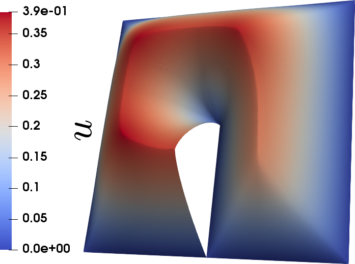
Figure 4: The domain $\Omega$ with boundary conditions (left) and the solution of the problem (right).

6.2.1 Integral evaluation

As first quantity of interest, we again consider $J(u)=\int_{\Omega}u(x)dx\approx 0.71755$. We observe in Figure 5 that we obtain a similar error for either solving the adjoint and primal problem each time (Error(full)), for using the interpolation on each level (Error(int)), and for Algorithm 1 (Error(new)).

As already noticed in [21], we observe higher-order convergence of the remainder term. The rate is approximately in the order of $\mathcal{O}(\text{DOFs}^{-\frac{3}{2}})$. For the errors and additionally the error estimator $\eta^{(2)}_{h}$, which is plotted for Algorithm 1, the order of convergence is approximately $\mathcal{O}(\text{DOFs}^{-1})$.

In Figure 6, the number of solves in the enriched space using Algorithm 1 divided by the number of solves in the enriched space using the algorithm given in [21] is shown. We conclude that, on the first seven levels, the same solves as from [21] are required. Then Algorithm 1 decides that we just have to solve either the primal or the adjoint problem on the enriched space, and use the interpolation in the other. After level $\ell=15$ only interpolation is used. Going back to Figure 5, we observe that, on the levels $\ell=8-12$, the error for just using interpolation is slightly worse than for the other approaches. However, on finer levels this effect does not appear anymore. Excellent effectivity indices are observed as visualized in Figure 7. For the full estimater, we observe almost no differences to the other versions proposed. In the case of Algorithm 1, the efficiency index $I_{eff}$ is approximately equal to $1.25$ when using interpolation only.

If we compare the different meshes, which are visualized in Figure 8, then we detect that, even after $28$ adaptive refinements, we end up in almost coinciding meshes.

Figure 5: $p$-Laplace for $p=4$, $\varepsilon=10^{-10}$: Integral evaluation: Error and error estimators versus DOFs.

Figure 6: $p$-Laplace for $p=4$, $\varepsilon=10^{-10}$: Integral evaluation: ratio of solves up to level $\ell$. Here, $\mathfrak{z}_{\ell}$ describes the number of enriched adjoint solves needed up to level $\ell$, and $\mathfrak{u}_{\ell}$ describes the number of enriched primal solves needed up to level $\ell$.

Figure 7: $p$-Laplace for $p=4$, $\varepsilon=10^{-10}$: Integral evaluation: Effektivity idices.

Figure 8: The resulting meshes on level $\ell=29$ for: solving always the enriched spaces (left), using Algorithm 1 (middle), using interpolations on all levels (right).

6.2.2 Point evaluation

In this part, we consider the point evaluation $J(u)=u(x_{P})\approx 0.04501097$ as quantity of interest, where the point $x_{P}=-\frac{9}{10}(1,1)$ is also visualized in Figure 4. Inspecting Table 1, we observe that $\lim_{\ell\rightarrow\infty}I_{eff}=0$ due to the local refinement around the evaluation point as mentioned in Remark 3.6.

Furthermore, Table 1 shows that the effectivity indices $I_{eff,h}$ and $I_{eff}$, defined in (10), are both better for Algorithm 1 than for using interpolation on every level. It is a bit surprising that the efficiency indices $I_{eff,h}$ perform equally well. Moreover, $\mathfrak{z}_{\ell}$ and $\mathfrak{u}_{\ell}$ show that Algorithm 1 decides to solve the enriched problems on several levels.

In comparison with the algorithm proposed in our previous work [21], we save five times solving the primal problem on the enriched space, and 1 adjoint problem on the enriched space. In Figure 9, we observe that heavy refinement occurs around our evaluation point.

The position of the point was motivated by the singularity in the distance function, which is the first eigenfunction of the $p$-Laplacian for $p=\infty$; see [31, 11]. This singularity is also refined by our strategy, provided that it is sufficiently close to our point. The errors in the point evaluation are similar for interpolation and the new Algorithm 1.

Table 1: $p$-Laplace for $p=4$, $\varepsilon=10^{-10}$: Point evaluation: In the first part of the table, the levels are given. In the second part, we have the results for Algorithm 1, and in the third the results for using the interpolation on every level. $|V_{h}^{\ell}|$ gives the DOFs in the finite element space, and $|V_{h}^{\ell,(2)}|$ gives the number of elements in the corresponding enriched space. The values $\mathfrak{z}_{\ell}$ and $\mathfrak{u}_{\ell}$ describe the number of enriched solves required up to level $\ell$. In the third part, $\mathfrak{z}_{\ell}$ and $\mathfrak{u}_{\ell}$ are not presented since $\mathfrak{z}_{\ell}=\mathfrak{u}_{\ell}=0$.

	new							int
$\ell$	$|V_{h}^{\ell}|$	$|V_{h}^{\ell,(2)}|$	$I_{eff,h}$	$I_{eff}$	$\mathfrak{z}_{\ell}$	$\mathfrak{u}_{\ell}$	Error	$|V_{h}^{\ell}|$	$|V_{h}^{\ell,(2)}|$	$I_{eff,h}$	$I_{eff}$	Error
1	27	85	0.55	0.61	1	1	3.07E-02	27	85	0.18	0.29	3.07E-02
2	36	117	0.56	0.84	1	2	1.94E-02	36	118	0.48	0.78	1.95E-02
3	53	180	0.78	0.81	2	3	3.28E-03	53	180	1.12	1.41	3.28E-03
4	69	240	0.81	1.17	3	3	2.02E-03	69	240	0.55	1.17	2.02E-03
5	93	334	0.82	0.84	4	4	7.44E-04	93	334	0.85	1.21	7.44E-04
6	120	441	0.61	0.80	5	5	3.12E-04	123	453	1.75	0.66	3.25E-04
7	154	575	0.65	0.84	6	6	2.68E-04	167	626	1.33	0.45	1.55E-04
8	201	760	0.83	0.81	7	7	1.26E-04	215	815	0.58	0.45	1.55E-04
9	258	985	0.48	0.72	8	8	4.63E-05	275	1 051	0.78	0.02	1.09E-04
10	332	1 279	0.56	0.86	9	9	6.20E-05	356	1 370	0.69	0.03	6.28E-05
11	448	1 734	0.71	0.80	11	10	2.17E-05	468	1 810	0.78	0.06	2.86E-05
12	578	2 247	0.51	0.64	13	11	8.21E-06	602	2 334	0.61	0.02	3.04E-05
13	739	2 884	1.52	0.87	13	12	1.31E-05	790	3 082	0.71	0.04	1.59E-05
14	940	3 670	0.64	0.87	14	13	8.58E-06	1 014	3 973	1.18	0.07	8.74E-06
15	1 206	4 727	2.32	0.44	15	13	1.47E-06	1 300	5 109	0.54	0.12	5.60E-06
16	1 549	6 096	1.03	0.23	16	13	1.26E-06	1 701	6 696	1.76	0.17	1.45E-06
17	1 993	7 855	0.95	0.88	17	14	1.58E-06	2 196	8 658	2.52	0.09	1.58E-06
18	2 561	10 120	77.10	31.99	18	14	1.13E-08	2 831	11 181	1.52	0.09	1.60E-06
19	3 310	13 092	1.61	0.43	19	14	5.03E-07	3 642	14 419	3.94	0.41	4.01E-07
20	4 274	16 939	1.13	0.90	20	15	3.05E-07	4 728	18 734	922.58	54.95	1.16E-09
21	5 462	21 679	2.09	1.00	20	16	5.74E-07	6 089	24 164	2.98	0.03	2.72E-07
22	7 105	28 206	0.53	0.78	21	17	6.91E-08	7 913	31 433	3.16	0.02	2.01E-07
23	9 111	36 203	1.12	1.07	22	18	1.90E-07	10 237	40 698	2.93	0.02	1.57E-07
24	11 760	46 780	1.07	1.07	23	19	9.13E-08	13 214	52 569	2.08	0.05	1.53E-07
25	15 228	60 614	1.06	1.07	24	20	1.08E-07	17 122	68 164	1.41	0.02	1.80E-07

Figure 9: $p$-Laplace for $p=4$, $\varepsilon=10^{-10}$: Point evaluation: Mesh on level $\ell=25$.

6.3 Navier-Stokes benchmark problem

We now consider the stationary NS-benchmark problem NS2D-1; see [45]. The computational domain $\Omega$ is given by $(0,H)\times(0,2.2)\setminus\mathcal{B}$, where $H=0.41$, and $\mathcal{B}:=B_{\frac{1}{20}}(0.2,0.2)$ is nothing but a circle with center at $(0.2,0.2)$ and radius $\frac{1}{20}$. The problem reads as follows: Find $\textbf{u}:=(u,p)\in[H^{1}(\Omega)]^{2}\times L^{2}(\Omega)$ such that

$$-\nu\Delta u+(u\cdot\nabla)u-\nabla p= 0\qquad\qquad\text{in }\Omega,$$

$$\nabla\cdot u= 0\qquad\qquad\text{in }\Omega,$$

$$u= 0\qquad\qquad\text{on }\Gamma_{\text{no-slip}},$$

$$u= \hat{u}\qquad\qquad\text{on }\Gamma_{\text{inflow}},$$

$$\nu\frac{\partial u}{\partial\vec{n}}-p\cdot\vec{n}= 0\qquad\qquad\text{on }\Gamma_{\text{outflow}},$$

where $\nu=10^{-3}$. The boundary parts are given by $\Gamma_{\text{outflow}}:=(\{x=2.2\}\cap\partial\Omega)\setminus\partial(\{x=2.2\}\cap\partial\Omega)$, $\Gamma_{\text{inflow}}:=\{x=0\}\cap\partial\Omega$, and $\Gamma_{\text{no-slip}}:=\overline{\partial\Omega\setminus(\Gamma_{\text{inflow}}\cup\Gamma_{\text{outflow}})}$.

The inflow is described by $\hat{u}(x,y):=(3w(y)/10,0)$ with $w(y)=4y(H-y)/H^{2}$. The pressure is uniquely determined due to the do-nothing condition prescribed on $\Gamma_{\text{outflow}}$; see [29]. Our quantity of interest is given by the lift which is defined as

$$J(\textbf{u}):=500\int_{\partial\mathcal{B}}\left[\nu\frac{\partial u}{\partial\vec{n}}-p\vec{n}\right]\cdot\vec{e}_{2}\,\text{ d}s_{(x,y)},$$

where $\vec{e}_{2}=(0,1)$. The reference value $J(\textbf{u})=0.010618948146$ was taken from [40].

In the numerical simulations, we observed that the ‘if’ conditions (Step 6-7 and Step 9-10) in Algorithm 1 were entered, possibly multiple times, resulting in a significant improvement of the effectivity indices. In Table 2, these evaluations have the following correspondences to the previous algorithm:

1. Step 1 (Table 2) $\quad\widehat{=}\quad$ Step 4 (Alg. 1). For the computation of the estimators, we use $u_{h}^{\ell,(2)}=I_{u}^{(2)}u_{h}^{\ell}\in U_{h}^{\ell,(2)}$ and $z_{h}^{\ell,(2)}=I_{z}^{(2)}z_{h}^{\ell}\in V_{h}^{\ell,(2)}$.

2. Step 2 (Table 2) $\quad\widehat{=}\quad$ Step 6-7 (Alg. 1). For the computation of the estimators, we use $u_{h}^{\ell,(2)}=I_{u}^{(2)}u_{h}^{\ell}\in U_{h}^{\ell,(2)}$ and $z_{h}^{\ell,(2)}$ as the solution of the linear problem: Find $z_{h}^{\ell,(2)}\in V_{h}^{\ell,(2)}$ such that $\mathcal{A}^{\prime}(u_{h}^{\ell,(2)})(z_{h}^{\ell,(2)},v_{h}^{\ell,(2)})=J^{\prime}(u_{h}^{\ell,(2)})(v_{h}^{\ell,(2)})$.

3. Step 3 (Table 2) $\quad\widehat{=}\quad$ Step 9-10 (Alg. 1). For the computation of the estimators, we use $u_{h}^{\ell,(2)}$ as the solution of the non-linear problem  Find $u_{h}^{\ell,(2)}\in U_{h}^{\ell,(2)}$ such that $\mathcal{A}(u_{h}^{\ell,(2)})(v_{h}^{\ell,(2)})=\leavevmode\nobreak\ 0$ and $z_{h}^{\ell,(2)}$ as in the previous executed step.

4. Step 4 (Table 2) $\quad\widehat{=}\quad$ Step 6-7 (Alg. 1). For the computation of the estimators, we use $u_{h}^{\ell,(2)}$ as the solution of the non-linear problem: Find $u_{h}^{\ell,(2)}\in U_{h}^{\ell,(2)}$ such that $\mathcal{A}(u_{h}^{\ell,(2)})(v_{h}^{\ell,(2)})=\leavevmode\nobreak\ 0$, and $z_{h}^{\ell,(2)}$ as the solution of the linear problem: Find $z_{h}^{\ell,(2)}\in V_{h}^{\ell,(2)}$ such that $\mathcal{A}^{\prime}(u_{h}^{\ell,(2)})(z_{h}^{\ell,(2)},v_{h}^{\ell,(2)})=J^{\prime}(u_{h}^{\ell,(2)})(v_{h}^{\ell,(2)})$.

Table 2: Navier-Stokes benchmark problem: Evolution of the effectivity indices during the exectuion of Algorithm 1. In Step 1, we use higher-order interpolation to approximate $z_{h}^{(2)}$ and $u_{h}^{(2)}$. If Step 2 is executed, then we update $z_{h}^{(2)}$ by solving the adjoint problem where $u_{h}^{(2)}$ is the interpolation. After executing Step 3, we replace the interpolation of $u_{h}^{(2)}$ by the solution of primal problem on the enriched space. In Step 4, $z_{h}^{(2)}$ and $u_{h}^{(2)}$ are the solutions of the primal and adjoint problem on the enriched spaces, respectively. The sign X means that this step is not executed. Lines 6 and 9 of Algorithm 1 decide whether a step is execuded or not.

	Step 1 (interpolation)			Step 2 (compute $z_{h}^{(2)}$)			Step 3 (compute $u_{h}^{(2)}$)			Step 4 (compute $z_{h}^{(2)}$)
$\ell$	$I_{eff,h}$	$I_{eff,\mathcal{R}}$	$I_{eff}$	$I_{eff,h}$	$I_{eff,\mathcal{R}}$	$I_{eff}$	$I_{eff,h}$	$I_{eff,\mathcal{R}}$	$I_{eff}$	$I_{eff,h}$	$I_{eff,\mathcal{R}}$	$I_{eff}$
1	1.71	1.69	1.92	X	X	X	2.23	2.2	1.55	X	X	X
2	1.28	1.28	0.24	1.13	1.13	0.24	0.79	0.79	0.78	X	X	X
3	1.52	1.52	0.15	1.13	1.13	1.15	0.86	0.86	0.85	X	X	X
4	0.66	0.66	0.88	0.80	0.80	0.88	X	X	X	X	X	X
5	0.45	0.45	0.11	X	X	X	0.72	0.72	1.00	X	X	X
6	0.41	0.41	0.31	0.88	0.88	0.31	1.01	1.01	0.99	X	X	X
7	0.89	0.89	0.67	X	X	X	X	X	X	X	X	X
8	0.41	0.45	0.85	2.17	2.21	0.85	1.54	1.58	1.60	X	X	X
9	2.81	2.81	2.86	0.71	0.71	2.86	0.75	0.75	0.74	X	X	X
10	3.42	3.42	0.86	1.34	1.34	0.86	1.10	1.10	1.06	X	X	X
11	4.20	4.20	0.18	0.70	0.70	0.18	1.08	1.08	1.08	X	X	X
12	5.72	5.72	1.92	0.68	0.68	1.92	1.33	1.33	1.35	X	X	X
13	3.49	3.49	0.40	0.62	0.62	0.40	X	X	X	X	X	X
14	5.11	5.11	1.63	X	X	X	5.97	5.97	0.38	0.38	0.38	0.38
15	2.16	2.16	1.61	X	X	X	1.99	1.99	0.94	0.94	0.94	0.94
16	1.50	1.50	1.70	1.29	1.29	1.70	X	X	X	X	X	X
17	6.25	6.24	1.95	1.30	1.29	1.95	1.59	1.58	1.58	X	X	X
18	109.0	109.2	10.3	6.71	6.88	10.3	2.17	2.34	2.27	X	X	X
19	47.7	47.7	4.75	5.35	5.35	4.75	X	X	X	X	X	X
20	231.0	231.0	2.87	X	X	X	226.4	226.4	2.93	2.95	2.93	2.93
21	20.7	20.7	14.1	X	X	X	2.10	2.09	2.10	X	X	X

Table 2 shows that we almost always improve the effectivity step by step. We notice that $I_{eff}$ does not depend on the choice of $z_{h}^{(2)}$ since it coincides for Step 1 and Step 2 as well as for Step 3 and Step 4 provided that these steps are executed. Furthermore, we observe that, in certain meshes, the use of interpolation leads to very bad effectivity indices. However, Algorithm 1 improves this during the adaptive process, although the saturation assumption is not fulfilled. The saturation assumption is also not fulfilled if $u_{h}^{(2)}$ is the exact discrete solution of the enriched space as shown in [21].

In Figure 11, we monitor a similar quality of the effectivity indices for new and full. Here we observe that the interpolation error estimator delivers a worse result. The resulting meshes for $\ell=20$ are shown in Figure 10. Here also the meshes of new and full are more similar. This is not surprising since we perform more enriched solves. For the error, which is discussed in Figure 12, a particular conclusion could not be determined.

Figure 10: Navier-Stokes benchmark problem: The corresponding meshes for $\ell=20$ and new(top), full(middle), int(bottom).

Figure 11: Navier-Stokes benchmark problem: Effektivity indices.

Figure 12: Navier-Stokes benchmark problem: Errors versus DOFs

7 Conclusions

We derived adaptive algorithms for computationally attractive low-order finite elements and interpolations to realize goal-oriented a posteriori error estimation using the DWR approach. Using saturation assumptions, we rigorously proved two-side error estimates showing the efficiency and robustness. These findings were supported by means of three numerical tests. Therein, the newly suggested error estimator was compared to the full estimator and a version in which only interpolations are used. For linear problems (Example 1), all three variants coincide with respect the error behaviour. For nonlinear problems (Example 2), differences can be observed. In the last numerical test (Example 3), a fluid-flow example was considered. Here, the PDE is semi-linear, but due to the convection term, the saturation assumption is not always fulfilled. This could be observed in terms of bad effectivity indices every now and then. Moreover, in the last example, the mechanism of our proposed adaptive algorithm is highlighted because the switch from interpolations to enriched spaces in some iterations significantly improves the effectivity indices. In future work, we plan to apply this algorithm to other applications, in particular, to multiphysics problems.

8 Acknowledgments

This work has been supported by the Austrian Science Fund (FWF) under the grant P 29181 ‘Goal-Oriented Error Control for Phase-Field Fracture Coupled to Multiphysics Problems’. Furthermore, the first two authors would like to thank IfAM from the Leibniz Universtät Hannover (LUH) for the organization of their visit in Hannover in January 2020. The third author would like to thank RICAM for his supported visit in Linz in November 2019, and for funding from the Deutsche Forschungsgemeinschaft (DFG, German Research Foundation) under Germany’s Excellence Strategy within the Cluster of Excellence PhoenixD (EXC 2122).

References

- [1] B. Achchab, S. Achchab, and A. Agouzal. Some remarks about the hierarchical a posteriori error estimate. Numer. Methods Partia. Diff. Equ., 20(6):919–932, 2004.
- [2] A. Agouzal. On the saturation assumption and hierarchical a posteriori error estimator. Comput. Methods Appl. Math., 2(2):125–131, 2002.
- [3] G. Alzetta, D. Arndt, W. Bangerth, V. Boddu, B. Brands, D. Davydov, R. Gassmöller, T. Heister, L. Heltai, K. Kormann, M. Kronbichler, M. Maier, J.-P. Pelteret, B. Turcksin, and D. Wells. The deal.II library, version 9.0. J. Numer. Math., 26(4):173–183, 2018.
- [4] W. Bangerth and R. Rannacher. Adaptive Finite Element Methods for Differential Equations. Birkhäuser Verlag, Boston, 2003.
- [5] R. E. Bank, A. Parsania, and S. Sauter. Saturation estimates for -finite element methods. Comput. Vis. Sci., 16(5):195–217, 2013.
- [6] R. E. Bank and R. K. Smith. A posteriori error estimates based on hierarchical bases. SIAM J. Numer. Anal., 30(4):921–935, 1993.
- [7] R. E. Bank and A. Weiser. Some a posteriori error estimators for elliptic partial differential equations. Math. Comp., 44(170):283–301, 1985.
- [8] R. Becker and R. Rannacher. Weighted a posteriori error control in FE methods. In e. a. H. G. Bock, editor, ENUMATH’97. World Sci. Publ., Singapore, 1995.
- [9] R. Becker and R. Rannacher. An optimal control approach to a posteriori error estimation in finite element methods. Acta Numer., 10:1–102, 2001.
- [10] F. A. Bornemann, B. Erdmann, and R. Kornhuber. A posteriori error estimates for elliptic problems in two and three space dimensions. SIAM J. Numer. Anal., 33(3):1188–1204, 1996.
- [11] F. Bozorgnia. Convergence of inverse power method for first eigenvalue of p-laplace operator. Num. Func. Anal. Opt., 37(11):1378–1384, 2016.
- [12] M. Braack and A. Ern. A posteriori control of modeling errors and discretization errors. Multiscale Model. Simul., 1(2):221–238, 2003.
- [13] C. Carstensen, D. Gallistl, and J. Gedicke. Justification of the saturation assumption. Numer. Math., 134(1):1–25, 2016.
- [14] P. G. Ciarlet. Finite Element Method for Elliptic Problems. Society for Industrial and Applied Mathematics, Philadelphia, PA, USA, 2002.
- [15] T. A. Davis. Algorithm 832: Umfpack v4.3—an unsymmetric-pattern multifrontal method. ACM Trans. Math. Softw., 30(2):196–199, June 2004.
- [16] A. De Rossi. Saturation assumption and finite element method for a one-dimensional model. RGMIA Research Report Collection, 5(2):Article 13, 1–6, 2002.
- [17] W. Dörfler and R. H. Nochetto. Small data oscillation implies the saturation assumption. Numer. Math., 91(1):1–12, 2002.
- [18] M. Duprez, S. P. A. Bordas, M. Bucki, H. P. Bui, F. Chouly, V. Lleras, C. Lobos, A. Lozinski, P.-Y. Rohan, and S. Tomar. Quantifying discretization errors for soft tissue simulation in computer assisted surgery: A preliminary study. Appl. Math. Model., 77:709–723, 2020.
- [19] B. Endtmayer, U. Langer, I. Neitzel, T. Wick, and W. Wollner. Multigoal-oriented optimal control problems with nonlinear pde constraints. Comput. Math. Appl., to appear, 2020.
- [20] B. Endtmayer, U. Langer, and T. Wick. Multigoal-oriented error estimates for non-linear problems. J. Numer. Math., 27(4):215–236, 2019.
- [21] B. Endtmayer, U. Langer, and T. Wick. Two-Side a Posteriori Error Estimates for the Dual-Weighted Residual Method. SIAM J. Sci. Comput., 42(1):A371–A394, 2020.
- [22] B. Endtmayer and T. Wick. A Partition-of-Unity Dual-Weighted Residual Approach for Multi-Objective Goal Functional Error Estimation Applied to Elliptic Problems. Comput. Methods Appl. Math., 17(4):575–599, 2017.
- [23] C. Erath, G. Gantner, and D. Praetorius. Optimal convergence behavior of adaptive FEM driven by simple (h-h/2)-type error estimators. ArXiv e-prints, May 2018.
- [24] A. Ern and M. Vohralík. Adaptive inexact Newton methods with a posteriori stopping criteria for nonlinear diffusion PDEs. SIAM J. Sci. Comput., 35(4):A1761–A1791, 2013.
- [25] L. Failer and T. Wick. Adaptive time-step control for nonlinear fluid-structure interaction. J. Comp. Phys., 366:448 – 477, 2018.
- [26] M. Feischl, D. Praetorius, and K. G. van der Zee. An abstract analysis of optimal goal-oriented adaptivity. SIAM J. Numer. Anal., 54(3):1423–1448, 2016.
- [27] S. Ferraz-Leite, C. Ortner, and D. Praetorius. Convergence of simple adaptive Galerkin schemes based on error estimators. Numer. Math., 116(2):291–316, 2010.
- [28] R. Hartmann. Multitarget error estimation and adaptivity in aerodynamic flow simulations. SIAM J. Sci. Comput., 31(1):708–731, 2008.
- [29] J. G. Heywood, R. Rannacher, and S. Turek. Artificial boundaries and flux and pressure conditions for the incompressible Navier-Stokes equations. Int. J. Numer. Meth. Fl., 22(5):325–352, 1996.
- [30] M. Holst and S. Pollock. Convergence of goal-oriented adaptive finite element methods for nonsymmetric problems. Numer. Methods Partia. Diff. Equ., 32(2):479–509, 2016.
- [31] B. Kawohl and J. Horák. On the geometry of the p-laplacian operator. Discrete Cont. Dyn.-S, 10(4), 2017.
- [32] U. Köcher, M. P. Bruchhäuser, and M. Bause. Efficient and scalable data structures and algorithms for goal-oriented adaptivity of space–time FEM codes. SoftwareX, 10:100239, 2019.
- [33] S. Korotov, P. Neittaanmäki, and S. Repin. A posteriori error estimation of goal-oriented quantities by the superconvergence patch recovery. J. Numer. Math., 11(1):33–59, 2003.
- [34] M. Maier and R. Rannacher. A duality-based optimization approach for model adaptivity in heterogeneous multiscale problems. Multiscale Model. Simul., 16(1):412–428, 2018.
- [35] G. Mallik, M. Vohralik, and S. Yousef. Goal-oriented a posteriori error estimation for conforming and nonconforming approximations with inexact solvers. J. Comput. Appl. Math., 366:112367, 2020.
- [36] S. A. Mattis and B. Wohlmuth. Goal-oriented adaptive surrogate construction for stochastic inversion. Comput. Methods Appl. Mech. Engrg., 339:36 – 60, 2018.
- [37] C. Mehlmann and T. Richter. A goal oriented error estimator and mesh adaptivity for sea ice simulations. arXiv preprint arXiv:2002.04350, 2020.
- [38] D. Meidner, R. Rannacher, and J. Vihharev. Goal-oriented error control of the iterative solution of finite element equations. J. Numer. Math., 17(2):143–172, 2009.
- [39] D. Meidner and T. Richter. Goal-oriented error estimation for the fractional step theta scheme. Comput. Methods Appl. Math., 14(2):203–230, 2014.
- [40] G. Nabh. On high order methods for the stationary incompressible Navier-Stokes equations. Interdisziplinäres Zentrum für Wiss. Rechnen der Univ. Heidelberg, 1998.
- [41] J. T. Oden. Adaptive multiscale predictive modelling. Acta Numer., 27:353–450, 2018.
- [42] R. Rannacher and J. Vihharev. Adaptive finite element analysis of nonlinear problems: balancing of discretization and iteration errors. J. Numer. Math., 21(1):23–61, 2013.
- [43] R. Rannacher, A. Westenberger, and W. Wollner. Adaptive finite element solution of eigenvalue problems: balancing of discretization and iteration error. J. Numer. Math., 18(4):303–327, 2010.
- [44] T. Richter and T. Wick. Variational localizations of the dual weighted residual estimator. J. Comput. Appl. Math., 279:192–208, 2015.
- [45] M. Schäfer, S. Turek, F. Durst, E. Krause, and R. Rannacher. Benchmark computations of laminar flow around a cylinder. In Flow simulation with high-performance computers II, pages 547–566. Springer, 1996.
- [46] P. Stolfo, A. Rademacher, and A. Schröder. Dual weighted residual error estimation for the finite cell method. J. Numer. Math., 27(2), 2019.
- [47] E. H. van Brummelen, S. Zhuk, and G. J. van Zwieten. Worst-case multi-objective error estimation and adaptivity. Comput. Methods Appl. Mech. Engrg., 313:723–743, 2017.
- [48] R. Verfürth. A review of a posteriori error estimation and adaptive mesh-refinement techniques. Advances in Numerical Mathematics. Wiley-Teubner, 1996.
- [49] S. Weißer and T. Wick. The Dual-Weighted Residual Estimator Realized on Polygonal Meshes. Comput. Methods Appl. Math., 18(4):753–776, 2018.
- [50] T. Wick. Goal functional evaluations for phase-field fracture using PU-based DWR mesh adaptivity. Comput. Mech., 57(6):1017–1035, 2016.