Evolutionary Models for 43 Galactic Supernova Remnants with Distances and X-ray Spectra

Abstract

The X-ray emission from a supernova remnant (SNR) is a powerful diagnostic of the state of the shocked plasma. The temperature (kT) and the emission measure (EM) of the shocked-gas are related to the energy of the explosion, the age of the SNR, and the density of the surrounding medium. Progress in X-ray observations of SNRs has resulted in a significant sample of Galactic SNRs with measured kT and EM values. We apply spherically symmetric SNR evolution models to a new set of 43 SNRs to estimate ages, explosion energies, and circum-stellar medium densities. The distribution of ages yields a SNR birth rate. The energies and densities are well fit with log-normal distributions, with wide dispersions. SNRs with two emission components are used to distinguish between SNR models with uniform ISM and with stellar wind environment. We find type Ia SNRs to be consistent with a stellar wind environment. Inclusion of stellar wind SNR models has a significant effect on estimated lifetimes and explosion energies of SNRs. This reduces the discrepancy between the estimated SNR birthrate and the SN rate of the Galaxy.

1 Introduction

Supernova remnants (SNRs) have a great impact in astrophysics, including injection of energy (e.g. Cox 2005) and newly synthesized elements into the interstellar medium (e.g. Vink 2012). Valuable constraints for stellar evolution and the evolution of the interstellar medium and the Galaxy can be obtained from SNR studies. The goals of SNR research include understanding explosions of supernovae (SN) and the resulting energy and mass injection into the interstellar medium.

Approximately 300 SNRs have been observed in our Galaxy by their radio emission (Green, 2019). Only a small number have been physically characterized, including determination of evolutionary state, explosion energy and age. Several historical SNR have modelled with hydrodynamic simulations (e.g. Badenes et al. 2006). Most SNRs have less complete observations than the historical SNRs, thus lack a definite age, and have not been modelled in detail. The non-historical SNRs are the main part of the Galactic SNR population. For many of these, a simple Sedov model with an assumed energy and ISM density has been applied. However, better modelling is required to derive energies, densities and ages from observations. Thus to study the physical properties of the SNR population it is necessary to use models simpler than full hydrodynamic modelling, but which include more physical effects than the Sedov model.

For the purpose of characterization of SNRs, we have developed a set of SNR models for spherically symmetric SNRs, which are based on hydrodynamic calculations. The most recent version of the models are described in Leahy et al. (2019). The model calculates temperatures and emission measures of the hot plasma, for forward-shocked and for reverse-shocked gas, based on hydrodynamic simulations. The resulting SNR models facilitate the process of using observations to estimate SNR physical properties.

This work includes the following. We extend the solution to the inverse problem, which calculates the initial parameters of a SNR from its observed properties, for the latest set of models in Leahy et al. (2019). We apply this inverse solution to a set of 43 SNRs with distances and with observed temperatures and emission measures. The structure of the paper is as follows. In Section 2 we present an overview of the SNR models and the solution of the inverse problem. In Section 3 the current sample of 43 SNRs is described. The results of model fits are given in Section 4 for 3 cases: with a standard model for all SNRs; with a cloudy SNR model for mixed morphology SNRs; and with a general model for two-component SNRs . In Section 5 we discuss the results, including statistical properties of the Galactic SNR population. The conclusions are summarized in Section 6.

2 SNR Evolution and Our Adopted Model

A SNR is the interaction of the SN ejecta with the interstellar medium (ISM). The various stages of evolution of a SNR are labelled the ejecta-dominated stage (ED), the adiabatic or Sedov-Taylor stage (ST), the radiative pressure-driven snowplow (PDS) and the radiative momentum-conserving shell (MCS). These stages are reviewed in, e.g., Cioffi et al. (1988), Truelove & McKee (1999) (hereafter TM99), Vink (2012) and Leahy & Williams (2017). In addition, there are the transitions between stages, called ED to ST, ST to PDS, and PDS to MCS, respectively. The ED to ST stage is important because the SNR is still bright, and it is long-lived enough that a significant fraction of SNRs are likely in this phase.

For simplicity our models assume that the SN ejecta and ISM are spherically symmetric. The ISM density profile is a power-law centred on the SN explosion, given by $\rho_{ISM}=\rho_{s}r^{-s}$, with s=0 (constant density medium) or s=2 (stellar wind density profile). The unshocked ejectum has a power-law density $\rho_{ej}\propto r^{-n}$. With these profiles, the ED phase of the SNR evolution has a self-similar evolution (Chevalier 1982 and Nadezhin 1985). The evolution of SNR shock radius was extended for the ED to ST and ST phases by TM99.

The model for SNR evolution that we use is partly based on the TM99 analytic solutions, with additional features. A detailed description of the model is given in Leahy et al. (2019) and Leahy & Williams (2017). We incorporate Coulomb collisional electron heating, consistent with the observational results of Ghavamian et al. (2013). The emission measure ($EM$) and emission measure-weighted temperature ($T_{EM}$) are calculated for ED, ED to ST and ST phases. $EM$ and $T_{EM}$ are calculated from the interior structure of the SNR from hydrodynamic simulations. $dEM_{FS}$, $dT_{FS}$, $dEM_{RS}$ and $dT_{RS}$ are calculated separately for forward shocked (FS) gas and for reverse shocked (RS) gas. Analytic fits in terms of piecewise powerlaw functions are made (Leahy et al., 2019) to the numerically determined $dEM_{FS}$, $dT_{FS}$, $dEM_{RS}$ and $dT_{RS}$. The inverse problem is solved, which takes as input the SNR observed properties and determines the initial properties of the SNR.

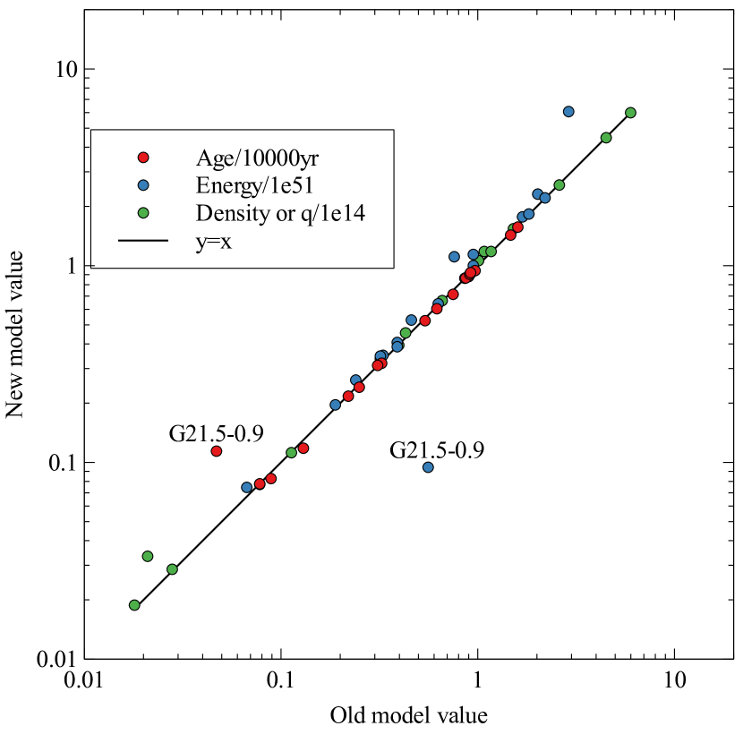
Figure 1: Comparison of fits using our new SNR model (Leahy et al., 2019) to fits using the older model for the 15 SNRs analyzed by Leahy & Ranasinghe (2018). Model inputs are radius, emission measure and temperature from Table 1 of Leahy & Ranasinghe (2018). Outputs are age, energy and density in both cases (see text for details). Table 4 of Leahy & Ranasinghe (2018) gives other inputs for the model: model type (forward shock or reverse shock), external density power-law (s=0 for ISM, s=2 for stellar wind), progenitor envelope power-law (n, in the range 6 to 14), and ejected mass. The “y=x” line indicates exact agreement between the two models. The outlier SNR G21.5-0.9 is discussed in the text.

To illustrate the changes in the current model (Leahy et al., 2019) compared to the model used by Leahy & Ranasinghe (2018), we recalculate the inverse models for the 15 SNRs in Leahy & Ranasinghe (2018). The main difference in the models is that our newer model includes accurate calculation of $dEM_{RS}$ and $dT_{RS}$ for the stages after the ED stage, rather than a simple linear interpolation. The parameters from the two models applied to the 15 SNRs are compared in Figure 1. Perfect agreement between the two models is indicated by the black line. The derived ages, energies and densities from the new model are very close to those from the previous simpler model. One clear exception is for the young SNR G21.5-0.9: there is a significant change in derived parameters because that SNR is in the ED to ST transition stage at a time where the difference between the newer accurate treatment and the previous linear interpolation is the largest.

2.1 The inverse problem: application of models to SNR data

The forward model, using initial SNR conditions and calculating conditions at time t, is described in Leahy et al. (2019). The input parameters of the SNR forward model are: age; SN energy $E_{0}$; ejected mass $M_{ej}$; ejecta power-law index n; ejecta composition; ISM temperature $T_{ISM}$; ISM composition; ISM power-law index s (0 or 2); and ISM density $n_{0}$ (if s=0) or mass-loss parameter $\rho_{s}=\frac{\dot{M}}{4\pi v_{w}}$ (if s=2). For Galactic SNRs, we take the ISM to be solar composition. We take the composition of ejecta and the mass of ejecta to be fixed, with values depending on the type of SN. For Type Ia we use $1.4M_{\odot}$ ejecta mass and for core-collapse (CC) or unknown type we use $5M_{\odot}$. We use the CC (for CC and unknown types) and Ia ejecta abundances from Leahy & Ranasinghe (2018). $T_{ISM}$ ,which doesn’t affect the evolution unless the SNR is very old, is set to 100 K. The resulting number of free parameters is 5 for the forward model.

The inverse model is solved by an iterative procedure. The observed FS radius ($R_{FS}$), FS emission measure ($EM_{FS}$) and FS EM weighted temperature ($T_{FS}$) for a given SNR are used to estimate ISM density, explosion energy and SNR age. The forward model is applied to calculate $R_{FS,model}$, $EM_{FS,model}$ and $T_{FS,model}$. Then the differences between the input and model value are used to determine new density, energy and age values. The process is repeated until the density, energy and age reproduce the input $R_{FS}$, $EM_{FS}$ and $T_{FS}$ to better than 1 part in $10^{4}$. To determine errors in the model parameters, the inverse solution is repeated for several sets of input parameters, for which the observed values are replaced in turn by their upper and lower limits.

To handle the fact that the inverse model has 3 input parameters, we apply the inverse solution for each $s$, $n$ case separately. For each fixed $s$, $n$ case there are 3 free parameters of the forward model (see first paragraph of this section). Thus, we can obtain a unique solution of SNR density, energy and age for each $s$, $n$.

Because the smooth dependence of the SNR models on $n$, we chose to limit the number of $n$ cases to $n=7$ and $n=10$. In cases where the observational data to distinguish these cases do not exist, we choose the $s=0$, $n=7$ model. In cases where observations on reverse-shocked ejecta exists, we choose the $s$, $n$ case which most closely reproduces the reverse shock properties ($EM_{RS}$ and $T_{RS}$).

3 The SNR Sample

The basic parameters of the SNRs were obtained from the catalogue of Galactic SNRs (Green, 2019) and the catalogue of High Energy Observations of Galactic Supernova Remnants (http://www.physics.umanitoba.ca/snr/SNRcat/ (Ferrand & Safi-Harb, 2012)). The SNRs were chosen to have reliable distances and X-ray observations. The average of major and minor axes (from Green (2019)) was used to estimate the average outer shock radius as input to the spherical SNR model.

Out of the 294 SNRs (Green, 2019), Leahy & Ranasinghe (2018) analysed 15 SNRs covered by the Very Large Array (VLA) Galactic Plane Survey (VGPS). The sample in the current work is comprised of 43 SNRs that lie outside the region that is covered by the VGPS. For each SNR, we obtained the temperature of the shocked gas from and calculated the emission measure from the reference for the X-ray spectrum and its spectral fit. For many cases, only a part of the SNR had an X-ray spectrum, so we had to extrapolate the given EM to account for the rest of the SNR. The EM values were adjusted from the published values, which assumed a distance, to the best-measured distance in the literature, and the dependence on distance is specified. In the next section are notes relevant to the modelling for each of the 43 SNRs, in order of increasing Galactic longitude. The adopted values of $EM$ and $kT$ are given in Table Evolutionary Models for 43 Galactic Supernova Remnants with Distances and X-ray Spectra.

We carry out three sets of models on the SNR sample. For the first set of models, we fit the data with a single hot plasma component, which is taken to be emission from gas heated by the forward shock (FS) and set $s=0$, $n=7$. The second set of models is applied for the subset of seven probable mixed morphology SNRs. For these SNRs a more appropriate model is that for a SNR in a cloudy ISM (White & Long 1991, hereafter WL). We have implemented this in our SNR modelling code, with the additional calculations of including electron-ion temperature equilibration, and of solving the inverse problem for the cloudy model. The third set of models is carried out for those 12 SNRs with two measured hot plasma components. The two components are likely from the forward shocked gas and the reverse shocked gas. The reverse shocked gas is identified by its enriched element abundances, if measured. For all 12 cases, the emission measure of the forward shocked, $EM_{FS}$, gas exceeds that of the reverse shocked gas. Thus, we choose $R_{FS}$, $EM_{FS}$ and $kT_{FS}$ as model inputs and compute predicted $EM_{RS}$ and $kT_{RS}$ for different $s$, $n$ cases.

3.1 Notes on Individual SNRs in the Sample

G38.7-1.4: This is a mixed morphology SNR and is large in radius, $\simeq$15 pc. The Chandra ACIS-I X-ray spectrum of G38.7-1.4 is well described by an absorbed non collisional-ionization-equilibrium (NIE) plasma model (Huang et al., 2014) with no evidence for RS heated ejecta. Based on the ACIS-I image, the spectral extraction area used by Huang et al. (2014) includes $\simeq$0.5 of the X-ray counts from the SNR, thus we multiply their EM by 2 to obtain an estimate of the total EM of the SNR.

G53.6-2.2: This is a large (radius $\simeq$35 pc), mixed morphology SNR. Broersen & Vink (2015) analyzed the ACIS-I X-ray spectrum of the whole SNR and found a two-component spectrum: one from FS-shocked ISM and one from RS-shocked ejecta

G67.7+1.8: This is a small (radius$\simeq$4 pc), mixed morphology SNR which likely hosts a central compact object (CCO). Hui & Becker (2009) extract ACIS-I spectra for the Northern Rim and the Southern Rim, and fit them with a collisional ionization equilibrium (CIE) model, finding significant enhancements in Mg, Si and S (at $\sim$ 3, 3 and 15 times solar abundance). Based on the ACIS-I image of the SNR and the given spectral extraction regions, we estimate $\simeq$0.33 of the X-ray flux of the SNR was included in the spectral extraction regions, so multiply their fit EM by a factor of 3 to obtain the total EM for the SNR.

G78.2+2.1: This was observed with ACIS-I and ACIS-S, with spectral and image analysis by Leahy et al. (2013). The NEI spectrum model APEC as fit to spectra of 5 different regions, which yields the mean temperature. The whole area of the SNR was not covered by the ACIS observations, so we use the norm of the APEC fit to the ROSAT whole SNR spectrum to obtain the EM.

G82.2+5.3/ W63: The X-ray spectrum was obtained with the ASCA GIS detector and analyzed with the VMEKAL model by Mavromatakis et al. (2004). The GIS data only covers a small central region of the SNR, so we use the ROSAT PSPC spectral fits of the southern area of the SNR to estimate a scaling factor of 10 to obtain the EM for the whole SNR.

G84.2-0.8: The X-ray spectrum was obtained with ACIS-I and analyzed by Leahy & Green (2012), using an APEC model. We compared the area observed in X-ray by ACIS-I with the radio image to estimate a scaling factor of 2.5 to obtain the EM for the whole SNR from the ACIS fit value.

G85.4+0.7 and G85.9-0.6: These two SNRs were observed using XMM Newton PN and MOS detectors and the spectra were analyzed by Jackson et al. (2008) using a VPSHOCK model. The spectrum extraction region encompasses the whole SNR in both cases so no adjustment to EM was necessary. Both G85.4+0.7 and G85.9-0.6 are mixed morphology SNRs.

G89.0+4.7/ HB21: The X-ray spectrum was obtained with ASCA SIS and GIS instruments by Lazendic & Slane (2006) and analyzed with the VNEI model. From the ROSAT PSPC image of G89.0+4.7, the flux outside of the ASCA spectrum extraction regions were estimated to yield a scaling factor of 2.0 to obtain the EM for the whole SNR.

G109.1-1.0/ CTB109: The spectrum was obtained with the Suzaku XIS instrument and analyzed by Nakano et al. (2015). The emission of the NE and SE regions, which avoids the bright central object 1E2259+586, was analyzed using a two component NEI plus VNEI model. The NEI model represented shocked ISM and was solar abundance; the VNEI model represented “shocked ejecta” and showed very mild enhancements of Si and S (by factors of 1.0 to 1.7). By examining the Suzaku XIS mosaic image of G109.1-1.0 and comparing the X-ray extraction regions to the radio image, we estimate a factor of 2.0 correction to obtain the EM for the whole SNR.

G116.9+0.2/ CTB 1: The ASCA SIS and GIS spectra of this mixed morphology SNR were analyzed by Lazendic & Slane (2006). The largest areas analyzed were called W-whole and NE-whole, and were fit with a two-component VRAY (CIE) model. The ROSAT PSPC image shows that the sum of X-ray emission of these two overlapping regions is exceeds the total X-ray emission of the SNR by about 50%, so we multiply the sum of the two EMs by 0.66 to estimate the total SNR EM.

G132.7+1.3/ HB3: This was observed in X-rays with ROSAT/PSPC, ASCA GIS and SIS and XMM-Newton pn detectors, and analyzed by Lazendic & Slane (2006) using a one-component VRAY model. Of the 5 overlapping regions, the 3 central regions show enhanced Mg abundance, by factor of $\simeq$2, and the central XMM-pn region shows additional O enhancement by factor of $\simeq$2. We use the average of temperature of all 5 regions and the ROSAT PSPC image to estimate the correction factor of 1.5 for EM, accounting for regions not covered by the spectra and accounting for the overlap of GIS, SIS and XMM-pn in the central region.

G156.2+5.7: Observations by the Suzaku XIS instrument were analyzed by Katsuda et al. (2009). The ROSAT PSPC image show the locations of the XIS fields on this X-ray shell-type SNR. Spectral parameters were derived using a VNEI model for the regions E1, E2, E3, E4 and NW4. The NW1, NW2 and NW3 regions were fit using two component VNEI +NEI or VNEI + power-law models. The central ellipse region was best fit using three component 2VNEI +NEI or 2VNEI + power-law models, with one of the VNEI components, with enhanced abundances of Si and S, identified as ejecta emission. We adopt the ejecta VNEI component from the central ellipse as the ejecta kT and EM. For the ISM component, we use the average temperature of the other regions. Katsuda et al. (2009) quote EM as the line-of-sight integral $EM_{los}=\int n_{e}n_{H}dl$, related to surface brightness, instead of the usual volume integral $EM=\int n_{e}n_{H}dV$, related to total SNR emission. The regions observed with Suzaku were of average surface brightness for this SNR, as determined by comparison with the ROSAT/PSPC image. Thus we average their $EM_{los}$ values (omitting the ejecta component), then convert to a total ISM EM using the area of X-ray emission for the whole SNR from the ROSAT/PSPC image.

G160.9+2.6/ HB9: This was observed by the ROSAT/PSPC and analyzed by Leahy & Aschenbach (1995). Table 2 gives best fit single component Raymond-Smith model spectral parameters for 7 regions covering the SNR. The average temperature and sum of the EMs was used for the total SNR emission.

G166.0+4.3/ VRO 42.05.01: This mixed morphology SNR was observed with Suzaku XIS instrument. X-ray spectra covering a large part of the NE region and a large part of the W region of the SNR were analyzed by Matsumura et al. (2017). Five different models were applied to the NE spectrum and one to the W spectrum. All models were the recombining plasma emission model VVRNEI, but differed in which abundances were assumed fixed at solar. We adopt the best fit models w-i and ne-iii, and use the average temperature and summed EM, with a correction by a factor of 1.4 for the emission from the SNR not covered by the X-ray extraction regions.

G260.4-3.4/ Puppis A/ MSH 08-44: This was observed with XMM-Newton MOS. Three regions (North, West and South) were extracted for spectral analysis by Katsuda et al. (2013). Their case A VNEI fits assumed Fe/H to be solar and gave better fits than their case B VNEI fits, which assumed O/H of 2000 times solar. The case A fits give enhanced O, Ne, Mg and Si by factors of $\simeq$3 to 10. We use the average T of the 3 regions. We sum the EMs, and use a correction factor of 2.0 to account for SNR emission outside the extraction regions, which was obtained from the Chandra ACIS-I image of the SNR.

G272.2-3.2: This is classified as a non-thermal composite SNR, and was observed with ASCA and ROSAT. The whole SNR spectrum from ASCA GIS and ROSAT PSPC was analyzed by Harrus et al. (2001) using a NEI model with no enhanced abundance. We adopt their T and EM to represent the shocked ISM for this SNR. Small regions A and B from the ASCA SIS were fit by the NEI model and gave similar T, and lower EM consistent with the smaller region size.

G296.7-0.9: This was observed by XMM-Newton MOS and analyzed by Prinz & Becker (2013). The spectrum of the X-ray bright SE rim was fit by various models, with the NEI, PSHOCK, SEDOV and GNEI models yielding good fits. We adopt the T and EM parameters from the NEI model, and correct the EM by a factor of 3.0 to account for the SNR emission outside the extraction region.

G296.8-0.3: The whole SNR was observed with XMM-Newton MOS and analyzed by Sánchez-Ayaso et al. (2012). Point-like sources were identified, including one object that is consistent with being a CCO, then excluded from the SNR elliptical extraction region. The resulting SNR spectrum was fit with a PSHOCK model, and we adopt those parameters.

G299.2-2.9: This is a type Ia SNR. Post et al. (2014) analyzed the Chandra ACIS-I spectrum of this SNR, using 4 small extraction regions labelled North(N), South(S), West(W) and Shell(Sh), and the VPSHOCK model. N, S and W are all interior to the rim, with N and S close to the center of the SNR. Enhanced abundances of Si S and Fe by factors of 4-8, 5-20, and 3-6, respectively, were found for N, S and W indicating the emission is from shocked ejecta. The Sh emission is taken as from shocked ISM. We use the Chandra image to estimate the correction factors to apply to both the ejecta and ISM components to get whole SNR values: $EM_{ej}\simeq 20EM_{ej,S}+20EM_{ej,N}+25EM_{ej,W}$ for the ejecta, and $EM_{ISM}\simeq 20EM_{ISM,S}+20EM_{ISM,N}+25EM_{ISM,W}+40EM_{ISM,Sh}$ for shocked ISM.

G304.6+0.1/ Kes 17 This was observed with ASCA GIS and SIS and analyzed by Pannuti et al. (2014). G304.6+0.1 was also observed with XMM Newton MOS1, MOS2 and PN instruments, and the extraction region covered the whole SNR. Various spectral models were fit by Pannuti et al. (2014), with the VAPEC plus power-law giving the best fit. This model had enhanced abundance of Mg by factor $\sim$10, and of Si and S by factors of $\sim$5. The filled center X-ray morphology indicates G304.6+0.1 is likely a mixed morphology SNR.

G306.3-0.9: This was observed with XMM Newton MOS1, MOS2 and pn, and with Chandra ACIS-I and ACIS-S (Combi et al., 2016). 3 X-ray point sources were excluded from the SNR spectra. Five extraction regions for the XMM-Newton data covered $\simeq$60% of the area of the SNR. MOS1, MOS2 and PN spectra were extracted for the five regions and fit with VAPEC plus VNEI models. The VAPEC component had mildly subsolar abundances and represents the shocked ISM component. The VNEI component for NE, NW, C and SW regions showed enhancements of Si, S Ar, Ca and Fe, by factors of 9-20 for NE, 2-9 for NW, 10-46 for C, 6-34 for SW and 1-2.6 for S. This indicates that all but region S are likely dominated by shocked ejecta emission. We adopt the VNEI for shocked ejecta component and VAPEC for shocked ISM component, and correct the EM by factor 2.0 for the area of the SNR outside the spectral extraction regions.

G308.4-1.4: This was classed as a mixed morphology SNR based on a low resolution ROSAT image. It was observed with Chandra ACIS-I at high resolution by Hui et al. (2012), showing it rather to be a limb-brightened partial shell SNR in X-rays. ACIS spectra were extracted for six regions: two Outer Rim regions, two Inner Rim regions and two Central regions. The regions pairs were combined for fitting and fit with an NEI model with similar T but much large EM for the Outer Rim, which is significantly brighter in X-rays. There is no evidence for enhanced abundances, so the emission is taken to be shocked ISM. We use the EM-weighted average of the temperatures. The EM was summed, with correction factor of 2 to account for the area and brightness outside the extraction regions, from the X-ray brightness image from Chandra.

G309.2-0.6: This was observed by the ASCA GIS and SIS instruments and analyzed by Rakowski et al. (2001). The SNR is shell type in radio, and centrally filled in X-rays. The ASCA SIS spectrum was modelled with a VNEI model, and showed enhanced Si abundance (factor $>$34) only, with other heavy elements (Ne through Fe) solar or subsolar. The abundances do not give a clear indicator of the SN type. The X-ray point source in G309.2-0.6 has absorption consistent with belonging to the foreground star cluster NGC5281, so is not likely a compact object associated with the SNR.

G311.5-0.3: The whole SNR was analyzed by Pannuti et al. (2017) using ASCA and XMM-Newton observations. The X-ray emission is centrally concentrated showing the SNR to be in the mixed morphology class. The ASCA GIS+SIS and XMM MOS1+MOS2+PN spectra were fit with an APEC model.

G315.4-2.3/ RCW86: This was observed with XMM-Newton with RGS and MOS instruments, and analyzed by Broersen et al. (2014). Analysis of X-ray line ratios with RGS was used to constrain T and ionization age $n_{e}t$ values for 4 different regions along the rim of the X-ray shell-type SNR. The RGS plus MOS spectra of 3 regions (SW, NW, SE) were fit with a two component VNEI model, one of low T and the second of high T, while the region NE was fit with a single low T VNEI component. The low T component showed mildly subsolar abundances, whereas the high T component showed enhanced O, Ne, Si and Fe, with variations. O and Ne were highest (18 and 3.5 times solar) for the SW region, Fe was highest for the NW region (24 times solar). We use the average T and sum of EMs for the low T component to represent shocked ISM and the average T and sum of EMs for the high T component to represent shocked ejecta. The EMs were further corrected, based on the X-ray image of the SNR, for the emission not included in the four spectral extraction regions, as follows: $EM_{total}\simeq 5EM_{NE}+2.5EM_{NW}+4EM_{SW}+6EM_{SE}$.

G322.1+0.0: This has been associated with the high mass X-ray binary Circinus X-1, thus is a CC type SNR. Chandra ACIS-I observations of G322.1+0.0 were analyzed by Heinz et al. (2013) showing a shell type SNR surrounding the bright central jet from Circinus X-1. The spectrum was fit with a SEDOV model. They quoted the line-of-sight $EM_{los}=\int n_{e}n_{H}dl$ which we converted to the usual volume integral $EM=\int n_{e}n_{H}dV$, using the area of the SNR.

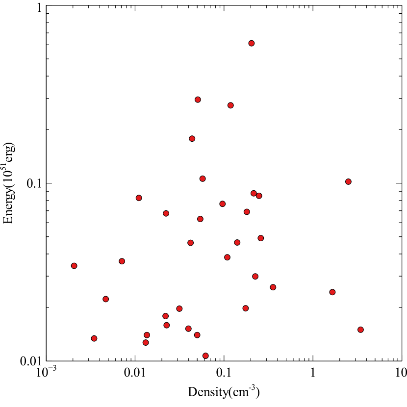
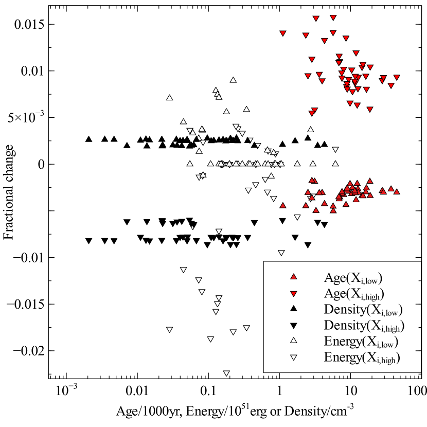
Figure 4: Left panel :Plot of energy vs. density for the Standard (s=0, n=7) models of the 43 SNRs. Right panel: Standard model run for the 43 SNRs with ISM abundances higher and lower than standard abundaces, by factor of $10^{0.5}$. The fractional change, defined as (new value - standard value)/standard value, is shown for age, density and explosion energy, and shown for the high abundance case (labelled $X_{i,high}$, downward pointing triangles) and for the low abundance case (labelled $X_{i,low}$, upward pointing triangles). All output values change less than 2% as ISM abundance is changed.

G327.4+0.4/ Kes 27:, was observed with the Chandra ACIS-I instrument and analyzed by Chen et al. (2008). It was previously thought to be a thermal composite-type SNR, but the Chandra image (Fig. 4 of Chen et al. 2008) shows a number of point sources and concentrations of bright diffuse emission much more consistent with a shell morphology in X-rays. 10 regions were chosen for spectrum extraction, along the rim and in the interior of the SNR to study spectral variations. The spectrum of the whole SNR was fit with XSPEC VPSHOCK and VSEDOV models. The latter gave a better fit and we adopt the parameters of that fit.

G330.0+15/ Lupus Loop: The whole SNR was observed by the HEAO-1 A2 LED detectors and analyzed by Leahy et al. (1991). We adopt the T and EM from the two-temperature Raymond-Smith model which was fit to the spectrum. The distance is highly uncertain, and could be as near as 500 pc or as far as SN1006, at 1.7 kpc (Leahy et al., 1991).

G330.2+1.0: This has a CCO and is a CC-type SNR with a clear shell of X-ray emission. XMM-Newton MOS1 and MOS2 and Chandra ACIS-I observations were analyzed by Park et al. (2009). Three small regions (NE, E and SW) were selected for extraction of spectra. SW and NE regions were fit with a power-law spectrum and E region was fit with pshock or a pshock plus power-law model. Thus, SW and NE regions are dominated by emission consistent with synchrotron, whereas E is consistent with shocked gas or a mixture of synchrotron and shocked gas emission. We adopt the parameters from the pshock plus power-law model. The ISM EM was corrected, based on the X-ray image of the SNR, for the emission not included in the E spectral extraction region: $EM\simeq 10EM_{E}$.

G332.4-0.4/ RCW 103: This was observed with Chandra ACIS-I and ACIS-S and analyzed by Frank et al. (2015). G332.4-0.4 is of shell type in X-rays and has a CCO. 27 regions were chosen for spectral analysis, and fit with a VPSHOCK model. The regions were classified as being dominated by shocked CSM (16 regions) or by shocked ejecta (11 regions). The ejecta regions were identified by enhancements in abundance of Mg, Si, S, or Fe. Typical abundances for the shocked ejecta regions had Ne in the range of 0.7-1.4 times solar, Mg 0.5-3.5 times solar, Si 0.5-4.6 times solar, S 0.4-1.5 times solar and Fe 0.8 to 6.8 times solar. The temperature of the shocked ISM and shocked ejecta were taken as the averages of T values for all regions for the shocked ISM component or shocked ejecta component, respectively. Frank et al. (2015) quote the line-of-sight $EM_{los}=\int n_{e}n_{H}dl$. Thus we obtain the $EM_{los,ej,av}$ of the shocked ejecta and $EM_{los,ISM,av}$ of the shocked ISM components by averaging the $EM_{los}$ values of ejecta or ISM for all regions. These are then converted to the usual volume integral $EM=\int n_{e}n_{H}dV$, using the area of the SNR.

G332.4+0.1/ MSH 16-51/ Kes 32: This was observed with Chandra ACIS-I (Vink, 2004). The SNR is shell-type in X-rays with a bright NW rim. Their second fit (Method 2) corrected for foreground diffuse Galactic emission, so we adopt the parameters of that fit. The spectral extraction region covered $\sim$1/3 of the area of the SNR and included the bright region, with only $\sim 10$% of the emission outside the extraction region. Thus, we apply a correction factor of 1.1 to obtain EM of the whole SNR.

G332.5-5.6: The central part was observed with the Suzaku XIS instrument (Zhu et al., 2015). The radio image shows three stripes of radio emission from the SNR shell. The central radio stripe is covered by the Suzaku XIS field of view and is coincident with the X-ray emission, indicating the X-ray emission is probably from the SNR shell. The XIS0 and XIS3 merged spectrum was fit with a VNEI plus power-law model. O, Mg and Fe abundances were fit, with the result that O and Fe were subsolar (at 0.6-0.8 times solar) and Mg was enhanced (1.2 times solar). Thus, the X-ray emission is consistent with shocked ISM. We apply a correction factor of 4 to EM to account for the area of the SNR not covered by the spectrum extraction region.

G337.2-0.7: This was observed with XMM-Newton MOS1, MOS2, PN and Chandra ACIS-S instruments (Rakowski et al., 2006). The whole SNR spectrum was obtained by fitting the data from all four detectors and fitting with a VNEI plus power-law model. Enhanced abundances for the VNEI component were derived for Ne, Mg, Si, S, Ar and Ca, with factors ranging from 1.7 to 12. This indicates that the emission is either from shocked ejecta or a combination of shocked ejecta and shocked ISM. Eleven small subregions ranging in location from rim to center were extracted for the four detectors. Each region was fit jointly (all four detectors) with a VNEI model, confirming that enhanced Si, S and Ca exists for all eleven subregions. The enhancements are more characteristic of a type Ia spectrum but the absence of enhanced Fe is harder to explain with a type Ia model (Rakowski et al., 2006).

G337.8-0.1/ Kes 41: This thermal composite was observed with XMM-Newton & Chandra (Zhang et al., 2015). An elliptical region covering the brightest X-ray emission near the center of the SNR was used for spectrum extraction for XMM MOS+PN and Chandra ACIS data. The spectra were fit jointly with a VNEI model with enhanced S and Ar abundances of 1.8 and 2.4 times solar, respectively. The small enhancements indicate the shocked gas is dominated by shocked ISM. We adopt their T and EM, with a correction factor of 2 to EM to account for emission outside the spectrum extraction area.

G347.3-0.5/ RX J1713.7-3946: This synchrotron-dominated SNR had its thermal spectrum detected by Katsuda et al. (2015) using XMM Newton MOS1+MOS2 and Suzaku XIS observations. A small region of $\simeq$4 arcmin radius near the center, but excluding the CCO, was used for spectrum extraction. We adopt their simultaneous spectral fit to MOS and XIS data using Model B with background region 2. The fit used the VVRNEI model and gave mildly enhanced abundances of Mg, Si and Fe, by factors of 2-4.3 times solar. Thus the emission is likely mainly from shocked ISM. They quote the line-of-sight $EM_{los}=\int n_{e}n_{H}dl$. Thus we convert to the usual volume integral $EM=\int n_{e}n_{H}dV$, using the area of the SNR.

G348.5+0.1/ CTB 37A: This was observed with XMM-Newton MOS1+MOS2+PN and Chandra ACIS-I detectors and analyzed by Pannuti et al. (2014). The MOS1+MOS2+PN spectrum was extracted for the whole of G348.5+0.1, excluding the small bright hard spectrum region CXOU J171419.8-383023. We adopt their best fitmodel which used a VAPEC model. The only element with non-solar abundance was Si with 0.48 times solar, indicating the emission is dominated by shocked ISM. The high resolution ACIS-I image shows the SNR to be of shell-type in X-rays. The ACIS-I spectra were extracted for CXOU J171419.8-383023, and the Northeast and Southeast rim of SNR G348.5+0.1. CXOU J171419.8-383023 had a power-law spectrum whereas Northeast and Southeast regions were fit with an APEC model that had T agree with the XMM-Newton spectrum fit and EMs each smaller by a factor $\simeq$4 than the total SNR EM, consistent with the smaller extraction region sizes.

G348.7+0.3/ CTB 37B: This was observed with Suzaku XIS and Chandra ACIS by Nakamura et al. (2009). The ACIS image shows the X-ray emission is separated into a point source plus diffuse emission. The diffuse emission is separated into two areas, region 1 and region 2 for both XIS and ACIS observations. Region 3 is seen in the XIS image but not in the ACIS image, so is likely a time variable active star. Region 1 and 2 have significantly more counts in the XIS observation, so the XIS data were used for spectral modelling, using a VNEI plus power-law spectra model. The T of region 1 and 2 are consistent with each other, and we sum the EMs and apply a small correction factor of 1.1 to account for emission outside the extraction regions.

G349.7+0.2 and G350.1-0.3: These two CC-type SNRs were observed with Suzaku XIS by Yasumi et al. (2014). The extraction region for both of these small angular sized SNRs included the whole SNR. The spectra of both remnants were fit with a solar abundance CIE component plus a VNEI component. For G349.7+0.2, the Mg and Ni abundances were found to be 3.6 and 7 times solar, while the other elements (Al, Si, S, Ar, Ca and Fe) were found to be either solar or sub-solar (0.6 to 1 times solar). For G350.1-0.3, all the abundances (Mg, Al, Si, S, Ar, C, Fe and Ni) were found to be above solar, with values ranging from 1.4 (Al and Fe) to 14 (for Ni). The CIE component is listed as the first component (shocked ISM) in Table Evolutionary Models for 43 Galactic Supernova Remnants with Distances and X-ray Spectra and the VNEI component is listed as the second component (shocked ejecta). However, the low abundances of the VNEI component for G349.7+0.2 indicate that the VNEI component my be a mixture of shocked ISM and ejecta.

G352.7-0.1: This was observed by XMM-Newton and Chandra and analyzed by Pannuti et al. (2014). With higher resolution than previous observations, the Chandra ACIS image show that this small angular diameter SNR is not centrally brightened but is more consistent with being an X-ray shell type remnant than a mixed morphology SNR. The Eastern and Whole SNR spectra were extracted from the XMM MOS1+MOS2+PN data and fit with a VNEI model. The Whole SNR spectrum showed enhanced Si and S with abundances 2.3-3.5 times solar, thus is likely a mixture of shocked ISM and shocked ejecta, and likely dominated by shocked ISM as pure shocked ejecta should have much larger abundances. Spectra were extracted for 6 regions plus a Whole SNR region from the ACIS data and were fit by a one component VNEI model, by a two component NEI + VNEI model, and by a two component VNEI+ VNEI model. The ACIS Whole region one component model yielded a T and EM consistent with the XMM spectrum fit and also showed enhanced Si and S abundances. The ACIS Whole region NEI+VNEI model was a significant improvement over the one component model. The cool NEI component was solar abundance and represents shocked ISM, whereas the hot VNEI component had Si and S enriched by factors of 3.4 and 9.4 over solar, so is likely dominated by shocked ejecta. The ACIS Whole region VNEI+VNEI model consisted of a hot Si-rich component (7 times solar) and a cool S-rich component (37 times solar), but the $\chi^{2}$ of the fit was not significanty better than the NEI+VNEI model. Thus, we adopt NEI+VNEI fit values here.

G355.6-0.0: This was observed by Suzaku (Minami et al., 2013). The Suzaku XIS image shows this SNR to be filled center, i.e. a mixed morphology SNR. The spectrum extraction region was 6^′ by 4^′ (major axes), smaller than the 8^′ by 6^′ SNR, but containing all the bright emission from the SNR. Thus we apply no correction factor to the EM. The background region was chosen to avoid the nearby bright X-ray emission from the star cluster NGC6383. We adopt the parameters from the spectrum fit using background $a$, which used a VAPEC model. This had Si, S, Ar and Ca enhanced by factors of 1.6, 3.1, 5.8 and 15 times solar, respectively. This may be a mixture of shocked ISM and shocked ejecta emission, but likely is dominated by shocked ejecta because of the high Ca abundance.

G359.1-0.5: The whole of this likely mixed morphology type was observed by Suzaku and analyzed by Ohnishi et al. (2011). One component CIE and two component CIE models did not well fit the XIS spectrum. One or two component underionized plasma models also did not fit the XIS spectrum of G359.1-0.5. An overionized plasma spectrum model was a significantly better fit, so we adopt the parameters from that model here. For that fit, Mg, Si and S were overabundant by factors of 3.4, 12, and 17, indicating that the component is consistent with being dominated by shocked ejecta.

4 Results of SNR Models

4.1 The Standard Model

For our standard case (Standard Model), we adopt $s=0$, $n=7$ for the ISM and ejecta density profiles. For known or suspected Type Ia SNRs we set the ejecta mass $M_{ej}$=1.4$M_{\odot}$, and for known or suspected CC SNRs we set $M_{ej}$=5$M_{\odot}$. Because the rate of CC type SNRs is several times higher than that of Ia type, the unknown types are more likely to be CC type. Thus we set $M_{ej}$=5 $M_{\odot}$ for unknown types. Further justification of the higher CC rate is found in the SNR types from Table Evolutionary Models for 43 Galactic Supernova Remnants with Distances and X-ray Spectra: 22 SNRs are type CC or CC? compared to 8 which are type Ia or Ia?. The results from applying this model are shown in Table 2. Derived ages, energies and densities and their uncertainties are given. Uncertainties were found by running models with the input parameters set to their upper and lower limits.

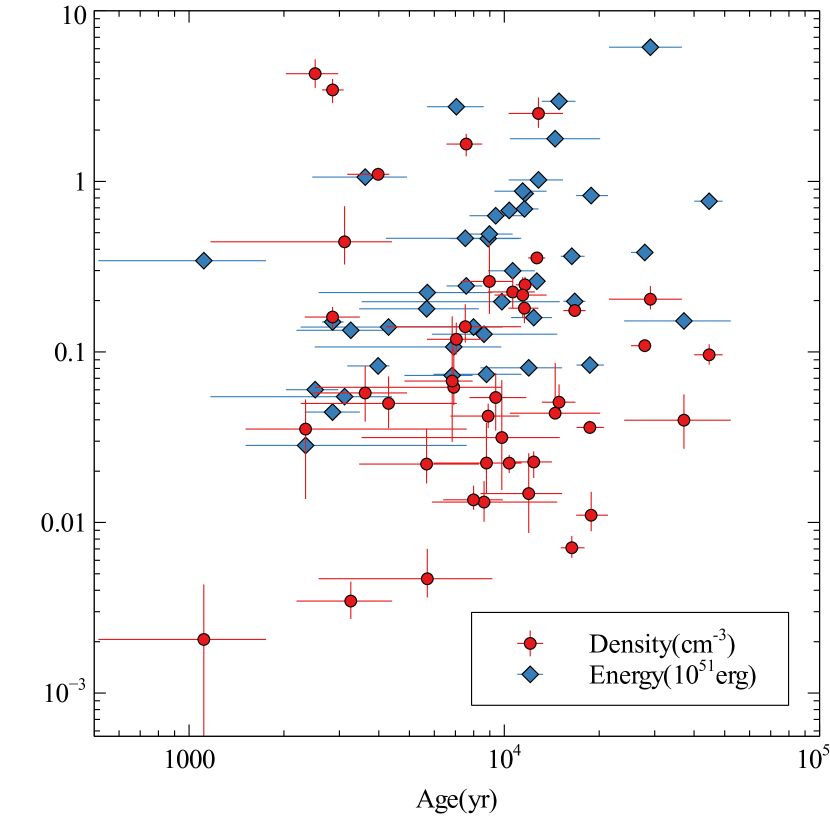
Figure 2: Model energies and densities vs. model ages derived from the standard model (forward shock from an SNR with ISM and ejecta profiles with $s=0$, $n=7$).

The SNR ages range from 1100 yr to 36000 yr; the explosion energies range from 0.03 to 6 $\times 10^{51}$ erg, and the ISM densities range from 0.002 to 4.3 cm^-3. Figure 2 shows the explosion energy and ISM density plotted as functions of SNR age. This illustrates the wide range of all three parameters and lack of correlation between them for the SNR sample. The results of the standard model are discussed in Section 5.1 below.

4.2 Mixed Morphology SNRs

Seven of the SNRs (G38.7-1.3, G53.6-2.2, G82.2+5.3, G166.0+4.3, G304.6+0.1, G311.5-0.3 and G337.8-0.1) are mixed morphology SNRs. For these we run the cloudy (WL) model with $C/\tau=2$ (called the WL2 model). The results are given in Table 3 and discussed in Section 5.2 below.

4.3 Two component SNRs

For 12 of the SNRs (see Table Evolutionary Models for 43 Galactic Supernova Remnants with Distances and X-ray Spectra), a second component is detected in the X-ray spectrum. This can be interpreted as reverse shock emission from the ejecta. These SNRs are G53.6-2.2, G109.1-1.0, G116.9+0.2, G156.2+5.7, G299.2-2.9, G306.3-0.9, G315.4-2.3, G330.0+15.0, G332.4-0.4, G349.7+0.2, G350.1-0.3 and G352.7-0.1. For the CC types and unknown types, we assume $M_{ej}$=5$M_{\odot}$ and CC-type ejecta abundances. For the Ia types, we assume $M_{ej}$=1.4$M_{\odot}$ and Ia-type ejecta abundances.

We apply our model to each of the 12 SNRs for 4 different cases of (s,n): (0,7), (0,10), (2,7) and (2,10). The model returns the age, energy and density required in order to reproduce the forward shock observed properties of $R_{FS}$, $EM_{FS}$ and $kT_{FS}$. From the SNR model we calculate the predicted reverse shock properties $EM_{RS}$ and $kT_{RS}$. Generally, the predicted EM-weighted reverse shock temperature decreases as n increases, and is larger for s=0 than s=2. In contrast, the predicted reverse shock emission measure increases as n increases, and is larger for s=2 than s=0. Table 4 show the results of applying SNR models for different (s,n) cases. The results from modelling the two-component SNRs are discussed in Section 5.4 below.

5 Discussion

5.1 Standard Model

5.1.1 Statistical properties

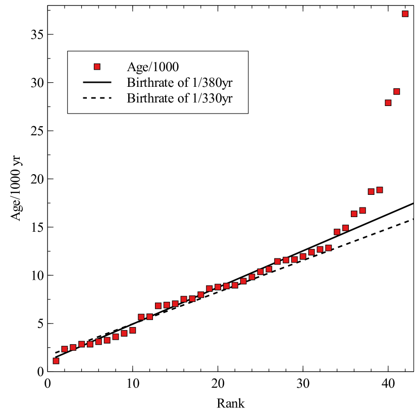
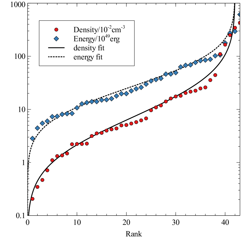
Figure 3: Left panel: Cumulative distribution of model ages from the standard model, and fit lines for birth rates of of 1 per 330 yr and 1 per 380yr. Right panel: Cumulative distributions of s=0, n=7 model explosion energies and of densities of the 43 SNRs. The fit lines are bset fit log-normal distributions. For explosion energies the mean is E₀=2.7$\times 10^{50}$ erg and variance in log(E₀) is 0.54. For densities the mean is $n_{0}$=6.9$\times 10^{-2}$ cm^-3 and variance in log($n_{0}$) is 0.71.

The statistical properties of the ages, explosion energies and ISM densities of the SNR sample are examined using an analysis similar to that carried out for the LMC SNR population by Leahy (2017) and for 15 Galactic SNRs (Leahy & Ranasinghe, 2018). The left panel of Figure 3 shows the cumulative distribution of model ages for our sample of 43 SNRs. The straight lines are the expected distributions for constant birth rates of 1/(330 yr) yr and 1/(380 yr), respectively. The fit lines have a non-zero x-intercepts of -5 and -3, respectively. This is equivalent to allowing for 5 or 3 missing young age ($\lesssim$ 1000 yr) SNRs in the sample. We note that we did not include the set of historical SNRs with age $\lesssim 1000$ yr in our age distribution, so the non-zero x-intercept is expected. Overall, a birthrate of 1/(350 yr) line is the best fit to the sample but values between 1/(380 yr) and 1/(330 yr) are consistent with the age distribution.

The cumulative distribution of explosion energies is shown in the right panel of Figure 3. This distribution is consistent with a log-normal distribution. The property that SNR explosion energies follow a log-normal distribution was discovered by Leahy (2017) and verified by Leahy & Ranasinghe (2018). Here, the best fit cumulative distribution has an average energy $E_{av}=2.7\times 10^{50}$ erg and dispersion $\sigma_{logE}$=0.54 (a 1-$\sigma$ dispersion factor of 3.5). These parameters are similar to those from the LMC SNR sample and from the 15 Galactic SNR sample.

The cumulative distribution of ISM densities is shown in the right panel of Figure 3. This distribution is consistent with a log-normal distribution, similar to that found by Leahy (2017) and Leahy & Ranasinghe (2018). The best fit cumulative distribution is shown by the solid line in Figure 3. The average density is $n_{0,av}=0.069$ cm^-3 and dispersion is $\sigma_{log(n_{0})}$=0.71 ( a 1-$\sigma$ dispersion factor of 5.1). For the LMC SNR sample, the mean density was similar and the dispersion was similar. The 15 Galactic SNRs subset (Leahy & Ranasinghe, 2018) has a higher mean density and similar dispersion. This is not surprising because the 15 Galactic SNRs were from the inner Galaxy where the density is expected to be higher.

5.1.2 Uncertainties and systematic effects

Some of the uncertainties of the analysis are mentioned here. We have taken spectral fit results from the literature, where different SNRs have observations made with different instruments, usually Chandra/ACIS, XMM/Newton MOS and PN, Suzaku XIS, or ASCA SIS and GIS instruments. There are effective area uncertainties of the different instruments, which are at a level of $\sim$10%. This can be compared to the errors in observed parameters of the SNRs. From Table Evolutionary Models for 43 Galactic Supernova Remnants with Distances and X-ray Spectra, distance and radius errors are typically 10 to 50%, EM errors are typically 10 to 50%, and kT errors typically 5 to 50%. Thus the observational errors dominate over instrument uncertainties.

In addition, many observations cover the whole SNR, but a significant number only cover a smaller region of the SNR. The correction factors to EM that we applied were based on the total counts of X-ray emission from the SNR which are inside and outside the spectral extraction region. A crude estimate of the error in correction factor, $f$, is $\sqrt{(}f)$, which for many SNRs with correction factor of $\sim$2 results in an estimate of $\sim$40% error. However, the counts in the X-ray image are better determined than this. E.g. typical SNR with 10,000 to 100,000 counts in the image has relative statistical error $\sqrt{(}10^{-4})=0.01$ to $\sqrt{(}10^{-4})=0.003$. Thus the statistical error in estimating $f$ is very small and the error in $f$ is dominated by systematic errors. Because the SNR measurement errors (see paragraph above) are large, they probably dominate over errors in $f$.

We examine some of the systematic effects that could be in the models, including sensitivity of model results to some of the changes in input assumptions. No correlation is expected between explosion energies and interstellar densities. The plot is shown in the left panel of Figure 4, using the Standard model results from Table 2. A least squares regression fit to energy vs. density yields a nearly flat line with a Pearson correlation coefficient of $R^{2}=0.0073$, thus no correlation is seen between the two quantities.

Next we consider the effect of changing the ISM abundances. The Standard model is run with a high abundance case with all elements except H and He elevated in abundance by a factor of $10^{0.5}$, and a a high abundance case with abundances decreased by the same factor compared to the standard solar ISM abundance. The results are shown in the right panel of Figure 4. The fractional change, defined as (new value - standard value)/standard value, is shown for age, density and explosion energy. For age, the high abundance case yields a $\sim 1.2$% increase, and low abundance yields a $\sim 0.4$% decrease. For density, the change is systematic with high abundance yielding a $-0.7$% change in ISM density and low abundance yielding a $+0.25$% change. For explosion energy, the high abundance case yields a $\sim 1.5$% decrease, and low abundance yields a $\sim 0$ to $\sim 0.8$% increase. All output values change less than 2% as ISM abundance is changed.

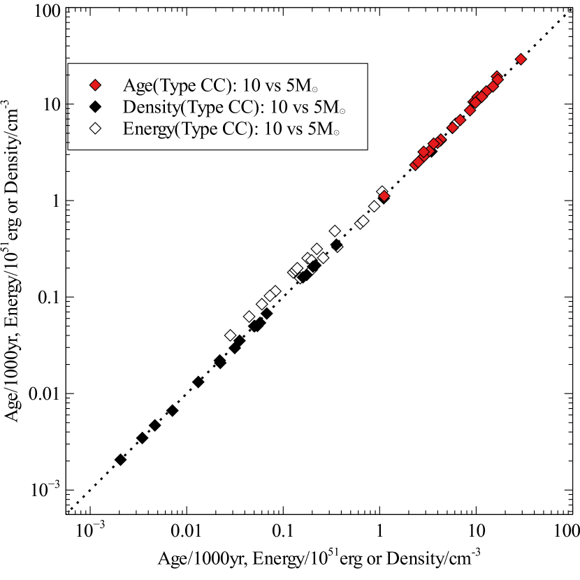
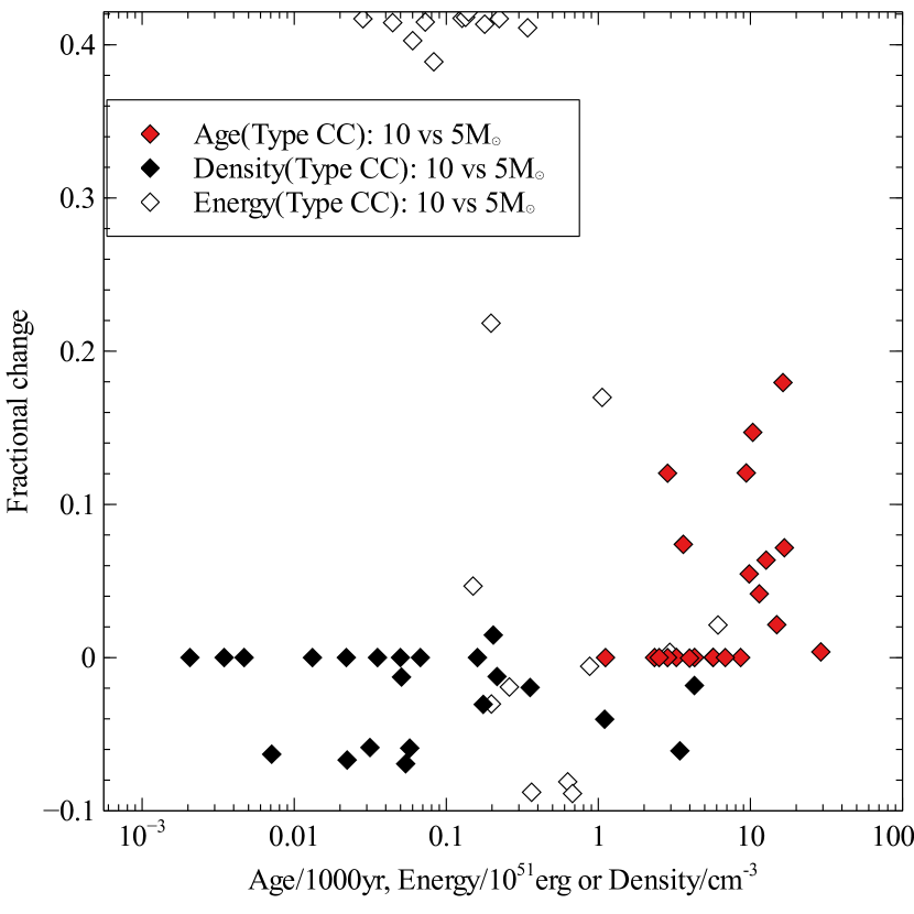
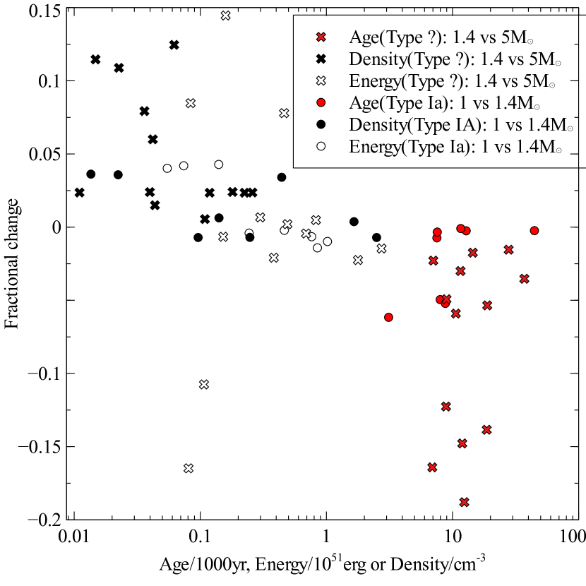
Figure 5: The effect of changing ejecta mass on the model outputs: The upper left panel is for Type CC SNRs: the age, density or energy with changed mass vs age, density or energy with standard mass. The upper right panel is for Type ? and Type Ia SNRs: the age, density or energy with changed mass vs age, density or energy with standard mass. (Lower left panel) the fractional change in age vs. age for the subset of 23 Type CC SNRs; the fractional change in density vs. density for Type CC; and the fractional change in energy vs. energy for Type CC. (Lower right panel) the fractional change in age vs. age for the subset of 13 unknown type (Type ?) SNRs and for the 8 Type Ia SNRs; the fractional change in density vs. density for Type ? and Type Ia; and the fractional change in energy vs. energy for Type ? and Type Ia.

The effect of changing the assumed ejecta masses is considered next. For this test, the mass for CC Type SNRs is increased from 5 to 10 $M_{\odot}$, for Type Ia SNRs is decreased from 1.4 to 1.0 $M_{\odot}$. For unknown types (Type ?), we change the mass from 5 to 1.4 $M_{\odot}$. The reason for the last change is to estimate the effect of having the Type ? as Type Ia instead of Type CC. The comparison of new age, density and explosion energy with the Standard model values is shown in the top panels of Figure 5. Type CC are on the left and Type ? and Type Ia are on the right. On these plots, the change in age, density or energy is small compared with their values so the values lie close to the line y=x. To examine the effect of changing ejecta mass more closely, the fractional changes for age, density and explosion energy are shown in the lower panels of Figure 5. Type CC are on the left and Type ? and Type Ia are on the right.

For Type CC SNRs, increasing ejecta mass from 5 to 10$M_{\odot}$ increases the age by 0 to 20%, with mean change of 4%. Increased ejecta mass decreases the ISM density by 0 to 7%, with mean decrease of 2%. The explosion energy has the largest change, from a 9% decrease to a 42% increase, with mean increase of 18% and large standard deviation of 20%. For Type Ia SNRs, decreasing ejecta mass from 1.4 to 1$M_{\odot}$ decreases the age by 0 to 6%, with mean decrease of 2%. The decreased ejecta mass changes the ISM density by -1 to +3.5%, with mean increase of 1.5%. The explosion energy for Type Ia has a change of -1 to +4.5% increase, with mean increase of 2%. For Type ? SNRs, decreasing ejecta mass from 5 to 1.4$M_{\odot}$ effectively assigns them as Type Ia instead of Type CC. This has the following effects. Age decreases by 2 to 19%, with mean decrease of 7%. The ISM density increases by 0 to 13%, with mean increase of 4%. The explosion energy has the largest change, from a 17% decrease to a 14% increase, with mean increase of 1%.

Overall, the change in mean age and mean ISM density for all three cases is small (between 1% and 4%), whereas the change in mean explosion energy is moderate (between 1% and 20%). The effect of changing ejecta mass has a negligible effect on the age and density distributions for our sample, shown in Figure 3. It has a small effect on the energy distribution. The energy distribution does not significantly change, and the derived parameters of the log-normal fit to explosion energies change to $E_{av}=3.0\times 10^{50}$ erg and dispersion $\sigma_{logE}$=0.53.

The different possible choices of SNR type, via choice of s and n, affect the output results of the model. This is discussed in detail in Leahy et al. (2019) and in Leahy & Williams (2017). For example, 8-9 different models are applied to each of three historical SNRs (Table 4 of Leahy et al. 2019). That work demonstrated that s=2 models are $\sim$5-10 times younger and their explosion energies are $\sim$10-100 times larger than for s=0 models. The ratio of emission measure of shocked ejecta to that of shocked ISM is much larger for s=2 models than for s=0. This large difference between s=0 and s=2 models allows one to distinguish between the two cases. For historical SNRs, the known age allows distinction. For SNRs of unknown age, one requires another quantity than age: a very useful one is the ratio of measured EM for shocked ejecta to EM for shocked ISM. In section 5.4 below we use SNRs with measured shocked ISM and shocked ejecta to distinguish whether the type is s=0 or s=2.

5.2 Cloudy ISM SNR Model

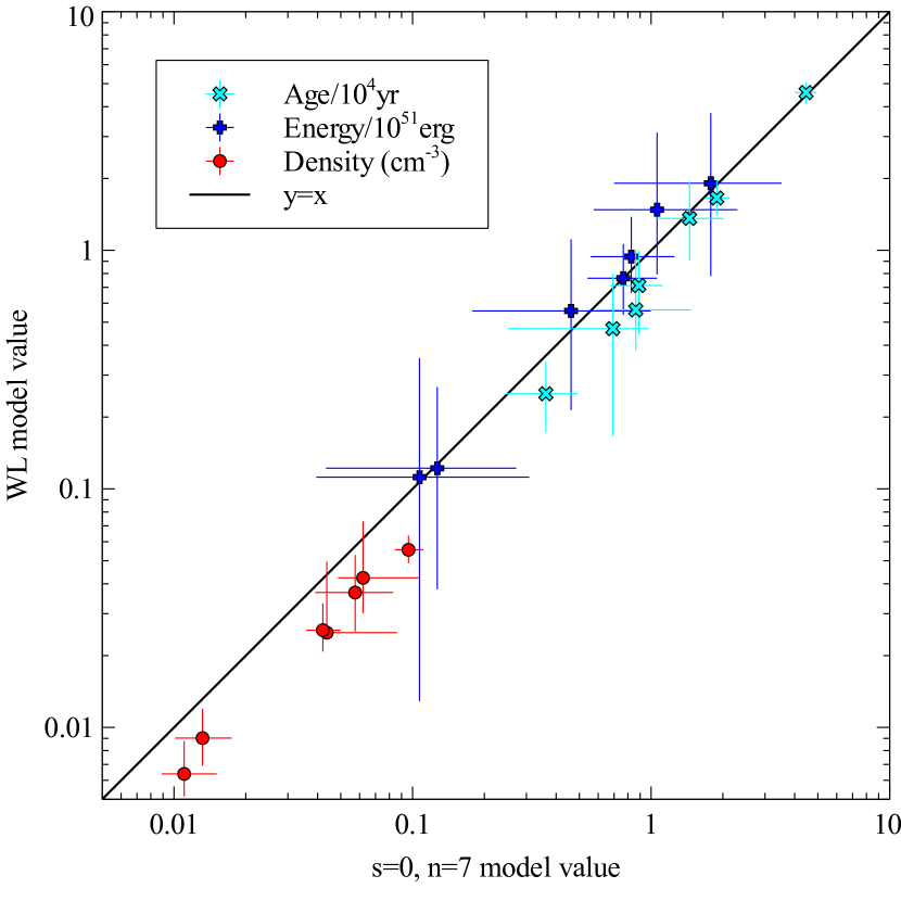
Figure 6: Comparison of ages, energies and densities of the 7 mixed morphology SNRs from the s=0, n=7 model and from the cloudy SNR (WL) model.

The resulting age, energy and density parameters are compared to those from the standard s=0, n=7 model in Figure 6. The ages and explosion energies are the same within errors for all 7 SNRs. The ISM density is lower for the WL model than for the s=0, n=7 model by a factor of $\simeq 1.5$. A lower derived ISM density for the WL model is expected because the WL model contains clouds. The clouds evaporate over the age of the SNR to increase the current post-shock density compared to what it would be without evaporation. This means that the initial ISM intercloud density is lower for the WL model than it would be for a standard uniform density ISM model.

5.3 Two component SNRs

We compare the predicted $EM_{RS}$ and $kT_{RS}$ of the different (s,n) cases with the measured values for each of the 12 SNRs to select a preferred model for each SNR. In choosing a preferred model, we attach more importance to reproducing $EM_{RS}$ and less to $kT_{RS}$. There are two reasons: i) uncertainties in the electron ion equilibration process for the reverse shock; ii) $kT_{RS}$ is more strongly affected than $EM_{RS}$ by the abundances in the ejecta (Leahy & Ranasinghe, 2018). Here, we assume fixed standard CC or Ia abundances rather than fine-tuning them. Instead we allow for differences of a factor of a few between the predicted and measured $EM_{RS}$ to indicate agreement. This is reasonable considering the several orders of magnitude difference in predicted $EM_{RS}$ from the different cases of (s,n) that we calculate.

The SNRs (with SN types labelled) which have the (s,n)=(0,7) model yield $EM_{RS}$ closest to the measured values are G116.9+0.2 (CC), G332.4-0.4 (CC?) and G350.1-0.3 (CC). None of the 12 SNRs have the (s,n)=(0,10) model yield the closest agreement. The SNRs which have the (s,n)=(2,7) model yield $EM_{RS}$ closest to the measured values are G109.1-1.0 (CC), G156.2+5.7 (CC), G330.0+15.0(?), and G349.7+0.2(CC). The SNRs which have the (s,n)=(2,10) model yield $EM_{RS}$ closest to the measured values are G53.6-2.2 (Ia), G299.2-2.9 (Ia), G306.3-0.9 (Ia), G315.4-2.3 (Ia) and G352.7-0.1 (Ia?).

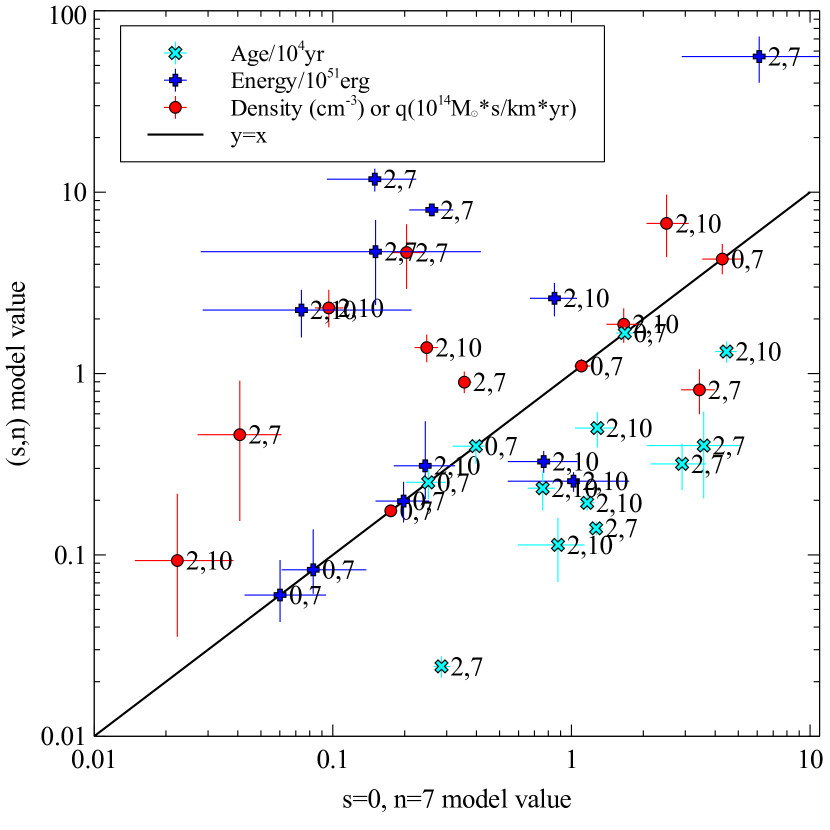
Figure 7: Ages, energies and densities of the preferred (s,n) models for each of 12 SNRs with two emission components. These are compared to the standard (s=0, n=7) model for each SNR. Each point is labelled with the preferred value of (s,n). In most cases, s=2 models work better than s=0 models. On average, the energies of the s=2 models are higher than the (0,7) model and the ages are smaller.

Figure 7 shows the results of our best (s,n) model for each of the 12 SNRs compared to the values from the standard (0,7) model. The ages and energies are directly compared. The ISM density, $n_{0}$ and the stellar wind parameter $q=\dot{M}/(4\pi V_{w})$ are plotted to show the wide range of $n_{0}$ (0.02 to 4 cm^-3) and $q$ ($10^{13}$ to $7\times 10^{14}$), although the $y=x$ line is not applicable.

Allowing for different s and n for each SNR makes a significant difference. We find that 9 of the 12 SNRs are more consistent with a stellar wind SN than an SN in a uniform ISM. This makes a large difference in the SN energy and SN age. For the 12 SNR (0,7) models, the mean log(age) and its standard deviation are 4.04 and 0.41, which decrease to 3.45 and 0.48, when individual customized (s,n) models are used. This is an average decrease by factor 3.9 in age. The mean log(energy) and standard deviation are 50.47 and 0.58, which increase to 51.05 and 0.94, when individual customized (s,n) models are used. This is an average increase by factor 3.8 in energy. A least squares fit of a log normal distribution to the energy values of the 12 SNRs yields a good fit with a mean log($E$) of 51.01 and $\sigma(log(E))$ of 1.08, consistent with the above values. These changes are large, and point to the importance of applying the correct type of SNR model when interpreting the measured values of $kT$ and $EM$. In particular, the statistics inferred for a SNR population when using only a s=0, n=7 model, may be offset to larger ages and lower explosion energies than using better (general s and n) models.

5.3.1 Type Ia SNRs with two component spectra

An important result that emerges from the models for two component SNRs, is that all five of the type Ia SNRs are consistent with stellar wind explosions and not with uniform density ISM explosions. This indicates that the origin of at least these five type Ia must be associated with a stellar wind. The stellar wind could be from a single WD accreting from a companion, or it could be binary WD merger if the merger occurs before the wind dissipates.

Previous work has found evidence for type Ia SNRs to be associated with stellar wind bubbles or cavities. Landecker et al. (1999) measured the HI environment of the probable type Ia SNR G93.3+6.9/DA530 and found it lies within a shell likely created by a stellar wind. Patnaude et al. (2012) study Kepler’s SNR with hydrodynamical and X-ray spectral modeling. They find neither uniform density nor pure $1/r^{2}$ wind profile fits but an explosion in a small cavity, indicative of some type of wind, gives consistency with observations. Broersen et al. (2014) use hydrodynamic simulations to find that G315.4-2.3/RCW 86 is a Type Ia explosion in a stellar wind cavity, as we find here. Zhou et al. (2016) study Tycho’s SNR using molecular line observations to detect an expanding clumpy bubble at the boundary of the SNR, likely the fast wind from an accreting WD progenitor.

The work here shows that to reproduce the measured ejecta $EM_{RS}$ and ISM $EM_{FS}$, s=0 models are ruled out and s=2 models favored for the type Ia SNRs. The current modelling of SNRs assumes spherical symmetry as an approximation to real SNRs. It is possible that more complex geometries, which do not require a stellar wind, could give give high ratio of ejecta EM to shocked-ISM EM. I.e., they could fit both measured $EM_{RS}$ and $EM_{FS}$ for type Ia SNR, like the s=2 models and unlike the s=0 models.

5.4 SNR birthrate and energetics

Most X-ray spectrum observations of SNRs do not yield two emission components, from forward shock and from ejecta. This can result from observations that are not sensitive enough, or if the SNR is old enough for the ejecta component to have faded below detection limits. For these SNRs we cannot constrain which (s,n) model fits better.

For the current set of 43 SNRs, we estimate the effect of having a subset of the SNRs in a stellar wind (s=2) rather than a uniform ISM (s=0) in two ways. First we use all of the SNRs from the current work and from Leahy & Ranasinghe (2018). The 43 SNRs consists of 34 with s=0 and 9 with s=2. The 15 SNRs of Leahy & Ranasinghe (2018) (Table 4 in that paper) had 13 with s=0 preferred and 2 with s=2 preferred. Thus, 11 of the 58 SNR models have a stellar wind environment.

Because a second EM is needed to decide if a s=2 model fits better than an s=0 model, the s=2 SNRs are all from SNRs with 2 measured EM components. Thus the above number gives a lower limit on the fraction of stellar wind SNRs. Using only 2 component SNRs, 2 of 5 SNRs from Leahy & Ranasinghe (2018) had s=2 and 9 of 12 in the current sample have s=2, giving a fraction of 11 of 17 with s=2. It is likely that this is an overestimate because s=0 SNRs have smaller ejecta EMs, thus are less likely to be included in the samples with 2 measured EMs.

Overall, we use 11/58 ($0.19\pm 0.06$) as the lower limit and 11/17 ($0.65\pm 0.20$) as the upper limit on fraction of SNRs in a stellar wind environment, including counting statistics error. The average of the upper and lower limits gives $0.42\pm 0.28$ as the best estimate of fraction of stellar wind SNRs. For 43 standard (s=0,n=7) models, we account for the presence of stellar wind SNRs using a fraction $\sim$0.4 which should be s=2 models. From Section 5.4, the s=2 ones have mean energy higher by a factor of 3.8 and mean age lower by a factor of 3.9 than s=0 models. This yields the mean energy for the log-normal distribution to be a factor $\sim$2 larger, and the mean age of the whole sample to be a factor $\sim$0.7 smaller. The estimated corrected explosion energy is $5\times 10^{50}$ erg and corrected SNR birth rate is 1/250 yr.

Because our sample is incomplete, a more complete survey of SNRs will increase the birth rate. We include the 15 Galactic SNRs from the sample of Leahy & Ranasinghe (2018), of which 13 have ages less than 10,000 yrs. Then our distribution of ages (similar to Figure 3 here) has a best-fit birth rate of 1/230 yr. If we further correct for expected fraction of stellar wind SNRs, the Galactic birth rate increases to 1/160 yr.

This rate is still significantly less than the SN rate in the Galaxy of 1 per 40$\pm 10$ yr (Tammann et al., 1994). The difference is primarily caused by incompleteness in SNRs measured in X-rays. Including the 58 Galactic SNRs with distances and X-ray spectra (this work and Leahy & Ranasinghe 2018) and comparing to the list of 294 SNRs (Green, 2019), we estimate an incompleteness factor of $\sim 5$. An alternate way to estimate the incompleteness is to consider the distribution of this sample of 43 SNRs with distance. A plot of cumulative number of SNRs vs. distance, $d$, shows a decrease from the expected $d^{2}$ increase for a disk-like distribution beyond a distance of $\sim$5 kpc. The area of the Galaxy, using most SNRs occur within $\sim$12 kpc of the center, to the area of a 5 kpc circle is $\sim$6, consistent with an incompleteness factor of $\sim$5 for SNRs measured in X-rays.

The net result is that the SNR birth rate corrected for incompleteness increases to $\sim$1 per 35 yrs. This latter rate is consistent with the estimated SN rate. This implies that there is no missing SNR problem, with large uncertainties, from statistics of X-ray detected SNRs.

Regardless of whether the incompleteness correction factor is overestimated or not, the ages of a significant fraction Galactic SNRs are overestimated. Many ages are estimated by using too-simplistic models, such as Sedov models with assumed energies and ISM densities. Leahy & Williams (2017) showed that Sedov models were significantly offset compared to more accurate TM99 models with the same input parameters. As shown in Leahy & Ranasinghe (2018), inclusion of $EM$ and $kT$ in modelling SNRs affects significantly estimates of ages and explosion energies. As shown here, inclusion of both uniform ISM and stellar wind SNR models has the important effect of increasing energies and decreasing ages compared to using only uniform ISM SNR models.

6 Conclusion

Distances to Galactic SNRs have improved significantly over the past decade, allowing determination of radii. X-ray observations of SNRs have been carried out for a significant fraction of Galactic SNRs. Together, these enable the application of SNR models to observed radii, emission measures and temperatures. We have improved the accuracy of spherically symmetric SNR evolution models by including results from a large grid of hydrodynamic simulations (Leahy et al., 2019). In the current study we apply the models to estimate SNR parameters for a sample of 43 Galactic SNRs. The distributions of the parameters were used to estimate properties of the Galactic SNR population. The energies and ISM densities of SNRs can be well fit with log-normal distributions in agreement with our earlier studies (Leahy 2017, Leahy & Ranasinghe 2018).

Seven of the 43 SNRs are mixed morphology SNRs. For these we apply WL cloudy ISM SNR models and compare the WL parameters to those estimated using our s=0, n=7 models. We find close agreement in parameters.

12 of the SNRs have two component X-ray spectra, indicating that both forward shocked material and reverse shocked ejecta are detected. With the extra information, we can distinguish between models with different s and n. We select the (s,n) model closest to the observations. One important finding is that all 5 of the 12 two-component SNRs that are type Ia are consistent with a stellar wind SNR. This has important implications for the progenitor types for these 5 type Ia SN: they should be consistent with a stellar wind environment.

A second important conclusion is that the inclusion of models for stellar wind SNRs is important when assessing the energies and ages of SNRs. We estimate that $\sim$40% of SNRs are stellar wind type, and the effect this has on SNR population ages and explosion energies. Including both uniform ISM and stellar wind SNR models has a significant effect on inferred mean ages of SNRs (a decrease by factor $\sim$0.7) and on inferred mean explosion energies of SNRs (an increase by factor of $\sim$2). After correction for stellar wind SNRs, we find a mean explosion energy of $\sim 5\times 10^{50}$ erg and a SNR birth rate of 1/260 yr for our population of 43 SNRs. Inclusion of the 15 Galactic SNRs from Leahy & Ranasinghe (2018) increases the birth rate to 1/160 yr. A final correction for the incompleteness of X-ray observations of SNRs increases the SNR birth rate to $\sim$1/35 yr, which is consistent with the Galactic SN rate (Tammann et al., 1994). To within uncertainties, this implies that there is no missing SNR problem when considering X-ray data.

This work was focussed on the population properties of Galactic SNRs by analyzing measured $EM$ and $kT$ from X-ray observations using of a basic set of SNR models. Future work will focus on individual SNRs where detailed consideration is given to observations at other wavebands to constrain better the choice SNR model (e.g., (s,n) parameters, ejecta mass and abundances).

Table 1: Observed Quantities of 43 SNRs

SNR	Type	Distance	Semi-axes	Radius	$EM^{a,b}$	$kT^{a,b}$	Refsf
		(kpc)	(arcmin)	(pc)	($10^{58}$cm-3)	(keV)
G38.7-1.3	CC?	4$\pm 0.8^{c}$	16$\times$9.5	14.9$\pm 3.0^{d}$	0.024(0.017-0.031)d${}_{4}^{2}$	0.65(0.35-0.95)	1, 1, 1
G53.6-2.2	Ia	7.8$\pm$0.8	16.5$\times$14	34.6$\pm$3.6	11.4(9.7-13.4)d${}_{7.8}^{2}$	0.14(0.13-0.15)	2, (3,4), 2
					0.022(0.015-0.030)d${}_{7.8}^{2}$	3.9(3.6-4.2)	-, -, 5
G67.7+1.8	CC?	2.0${}^{+3.7}_{-0.5}$	7.5$\times$6	4${}^{+7}_{-1}$	0.0033(0.0015-0.0056)d${}_{2}^{2}$	0.59(0.53-0.65)	6, 4, 6
G78.2+2.1	CC?	2.1$\pm 0.4$	30$\times$30	19$\pm$4	0.61(0.30-1.0)d${}_{2.1}^{2}$	0.83(0.62-1.0)	7, 7, 7
G82.2+5.3	?	3.2$\pm 0.4$	47$\times$32	37$\pm$4	0.184(0.132-.308)d${}_{3.2}^{2}$	0.63(0.59-0.68)	-, 4, 8
G84.2-0.8	?	6.0$\pm$0.2	10$\times$8	18$\pm$3	0.11(0.08-0.13)d${}_{6}^{2}$	0.58(0.49-0.66)	-, 9, 9
G85.4+0.7	CC?	3.5$\pm$1	12$\times$12	12$\pm$4	0.035(0.027-0.061)d${}_{3.5}^{2}$	0.86(0.81-0.90)	10, 11, 11
G85.9-0.6	Ia?	4.8$\pm$1.6	12$\times$12	17$\pm$5	0.030(.027-.036)d${}_{4.8}^{2}$	0.68(0.64-0.71)	10, 11, 11
G89.0+4.7	CC	1.9${}^{+0.3}_{-0.2}$	60$\times$45	31$\pm$4	0.051(.043-.064)d${}_{1.9}^{2}$	0.61(0.58-0.65)	12, 4, 13
G109.1-1.0	CC	3.1$\pm 0.2$	14$\times$14	12.6$\pm$0.9	7.5(7.1-8.0)d${}_{3.1}^{2}$	0.255(0.245-0.265)	14, 15, 16
					1.13(1.05-1.2)d${}_{3.1}^{2}$	0.64(0.63-0.68)	-, -, 17
G116.9+0.2	CC	3.1$\pm$0.3	17$\times$17	15.3$\pm$1.5	3.26(3.21-3.31)d${}_{3.1}^{2}$	0.22(0.19-0.25)	18, 19, 13
					0.0115(0.011-0.012)d${}_{3.1}^{2}$	0.84(0.78-0.93)	-, -, 20
G132.7+1.3	?	2.1$\pm$0.1	40$\times$40	24$\pm$1.2	4.72(4.67-4.77)d${}_{2.1}^{2}$	0.22(0.17-0.28)	-, 21, 13
G156.2+5.7	CC	2.5$\pm 0.8$	55$\times$55	38$\pm$10	67(66-68)d${}_{2.5}^{2}$	0.40(0.39-0.41)	22, 23, 22
					3.4(3.3-3.5)d${}_{2.5}^{2}$	0.51(0.50-0.52)	-, -, 22
G160.9+2.6	CC?	0.8$\pm$0.4	70$\times$60	16$\pm$8	0.0038(0.0034-0.0042)d${}_{0.8}^{2}$	0.82(0.76-0.88)	12, 24, 25
G166.0+4.3	?	4.5$\pm$1.5	27$\times$18	30$\pm$9	1.5(1.2-1.8)d${}_{4.5}^{2}$	0.8(0.5-1.1)	-, 26, 27
G260.4-3.4	CC	1.3$\pm$0.3	30$\times$25	10.5$\pm$3	0.00058(0.00046-0.00070)d${}_{1.3}^{2}$	0.79(0.66-0.92)	28, 29, 30
G272.2-3.2	Ia	6$\pm 4$	7.5$\times$7.5	14$\pm$7	1.57(1.49-1.65)d${}_{6}^{2}$	0.73(0.68-0.76)	31, 31, 32
G296.7-0.9	?	10$\pm 0.9$	7.5$\times$4	17$\pm$2	4.7(3.5-6.7)d${}_{10}^{2}$	0.53(0.46-0.60)	-, 33, 33
G296.8-0.3	CC?	9.6$\pm$0.6	10$\times$7	23.7$\pm$1.5	0.21(0.17-0.25)d${}_{9.6}^{2}$	0.86(0.85-0.87)	35, 34, 35
G299.2-2.9	Ia	5$\pm 1^{c}$	9$\times$5.5	14$\pm$5	0.046(0.025-0.10)d${}_{5}^{2}$	0.54(0.42-0.66)	36, 36, 37
					0.029(0.018-0.040)d${}_{5}^{2}$	1.36(1.28-1.45)	-, - ,37
G304.6+0.1	?	$>9.7^{e}$	4$\times$4	18$\pm$6	0.34(0.30-0.38)d${}_{15}^{2}$	0.84(0.75-0.95)	-, 38, 39
G306.3-0.9	Ia	20$\pm 4^{c}$	2$\times$2	11.6$\pm$2.3	290(240-350)d${}_{20}^{2}$	0.190(0.185-0.198)	40, 41, 42
					1.8(1.4-2.2)d${}_{20}^{2}$	1.51(1.31-1.71)	-, -, 42
G308.4-1.4	CC?	3.1$\pm 0.3$	6$\times$3	4.1$\pm$0.5	0.074(0.062-0.085)d${}_{3.1}^{2}$	0.68(0.52-0.87)	43, 44, 45
G309.2-0.6	CC?	2.8$\pm 0.8$	7.5$\times$6	8$\pm$4	9.E-5(1.E-5-2.0E-4)d${}_{2.8}^{2}$	2.0(1.4-3.0)	, 44, 46
G311.5-0.3	?	$>6.6^{e}$	2.5$\times$2.5	10$\pm$6	0.16(0.13-0.19)d${}_{13}^{2}$	0.68(0.44-0.88)	-,38, 47
G315.4-2.3	Ia	2.8$\pm 0.2$	21$\times$21	17$\pm$1.1	8.5(7.2-9.8)d${}_{2.8}^{2}$	0.5(0.44-0.56)	48, 49, 48
					0.046(0.037-0.056)d${}_{2.8}^{2}$	3.04(2.85-3.23)	, , 48
G322.1+0.0	CC	9.3$\pm 0.9$	4$\times$2.3	8.5$\pm$0.8	0.064(0.036-0.12)d${}_{9.3}^{2}$	0.9(0.5-1.7)	50, 50, 51
G327.4+0.4	?	4.3$\pm 0.8^{c}$	12$\times$11	13.1$\pm$2.7	3.4(2.6-4.2)d${}_{4.3}^{2}$	0.41(0.37-0.44)	-, 52, 53
G330.0+15.0	?	1$\pm 0.5$	90$\times$90	27$\pm$12	0.92(0.6-1.2)d${}_{1}^{2}$	0.135(0.13-0.14)	-, 54, 55
					0.15(0.08-0.22)d${}_{1}^{2}$	0.53(0.49-0.57)	-, -, 55
G330.2+1.0	CC	$>4.9^{e}$	5.5$\times$5.5	16$\pm$8	0.15(0.05-0.4)d${}_{10}^{2}$	0.7(0.4-2.0)	57, 56, 57
G332.4-0.4	CC	3.0$\pm 0.3^{c}$	5$\times$5	4.5$\pm$0.9	4.25(4.12-4.40)d${}_{3}^{2}$	0.57(0.53-0.61)	58, 44, 58
					0.51(0.47-0.54)d${}_{3}^{2}$	0.66(0.59-0.74)	-, -, 58
G332.4+0.1	?	9.2$\pm 1.7$	7.5$\times$7.5	20$\pm$4	3.3(2.4-4.2)d${}_{9.2}^{2}$	1.34(1.2-1.48)	-, 59, 59
G332.5-5.6	?	3.0$\pm 0.8$	18$\times$17	15.5$\pm$4	0.034(0.026-0.042)d${}_{3}^{2}$	0.49(0.43-0.57)	-, 60, 60
G337.2-0.7	Ia?	5.5$\pm 3.5$	3$\times$3	4.7$\pm$3	0.72(0.54-0.80)d${}_{5.5}^{2}$	0.74(0.73-0.77)	61, 62, 62
G337.8-0.1	CC?	12.3$\pm 1.2$	4.5$\times$3	13.4$\pm$1.3	0.29(0.15-0.54)d${}_{12.3}^{2}$	1.8(2.6-1.3)	63, 64, 63
G347.3-0.5	CC	1$\pm 0.2^{c}$	32$\times$28	8.8$\pm$1.7	0.13(0.03-0.60)d${}_{1}^{2}$	0.58(0.51-0.59)	65, 66, 65
G348.5+0.1	CC	7.9$\pm 1.6$	8$\times$7	17.2$\pm$3.5	6.9(4.5-9.0)d${}_{7.9}^{2}$	0.55(0.44-0.72)	67, 67, 39
G348.7+0.3	CC	13.2$\pm 1.3$	9$\times$8	32.8$\pm$3.3	2.6(1.9-3.8)d${}_{13.2}^{2}$	0.89(0.84-0.93)	67, 67, 68
G349.7+0.2	CC	11.5$\pm 1.2$	1.3$\times$1.0	3.7$\pm$0.4	21(16-26)d${}_{11.5}^{2}$	0.60(0.56-0.64)	61, 69, 70
					14(12.5-15.5)d${}_{11.5}^{2}$	1.24(1.21-1.27)	-, -,70
G350.1-0.3	CC	9$\pm 1.8^{c}$	2$\times$2	2.6$\pm$0.5	13(10-16)d${}_{9}^{2}$	0.48(0.44-0.52)	61, 70, 70
					1.2(1.0-1.4)d${}_{9}^{2}$	1.51(1.42-1.60)	-, -,70
G352.7-0.1	Ia?	7.5$\pm 0.5$	4$\times$3	7.6$\pm$0.5	34(26-42)d${}_{7.5}^{2}$	0.24(0.19-0.32)	61, 71, 72
					0.11(0.09-0.14)d${}_{7.5}^{2}$	3.2(2.4-4.6)	-, -,72
G355.6-0.0	?	13$\pm 2.6^{c}$	4$\times$3	13.2$\pm$2.7	4.6(2.3-10.0)d${}_{13}^{2}$	0.56(0.55-0.57)	-, 73, 73
G359.1-0.5	?	5$\pm 1^{c}$	12$\times$12	17.5$\pm$3.5	0.24(0.18-0.32)d${}_{5}^{2}$	0.29(0.27-0.31)	-, 74, 75

References. — (1) Huang et al. (2014), (2) Broersen & Vink (2015), (3) Giacani et al. (1998), (4) Shan et al. (2018), (5) Saken et al. (1995), (6) Hui & Becker (2009), (7) Leahy et al. (2013) , (8) Mavromatakis et al. (2004), (9) Leahy & Green (2012), (10) Kothes et al. (2001), (11) Jackson et al. (2008), (12) Boubert et al. (2017), (13) Lazendic & Slane (2006), (14) Nakano et al. (2017), (15) Sánchez-Cruces et al. (2018), (16) Nakano et al. (2015), (17) Sasaki et al. (2004), (18) Yar-Uyaniker et al. (2004), (19) Hailey & Craig (1994), (20) Pannuti et al. (2010), (21) Zhou et al. (2016), (22) Katsuda et al. (2009), (23)Katsuda et al. (2016), (24) Leahy & Tian (2007), (25) Leahy & Aschenbach (1995), (26) Landecker et al. (1989), (27) Matsumura et al. (2017), (28) Katsuda et al. (2018), (29) Reynoso et al. (2017), (30) Katsuda et al. (2013), (31) Sezer & Gök (2012), (32) Harrus et al. (2001), (33) Prinz & Becker (2013), (34) Gaensler et al. (1998), (35) Sánchez-Ayaso et al. (2012), (36) Park et al. (2007), (37) Post et al. (2014), (38) Caswell et al. (1975), (39) Pannuti et al. (2014), (40) Sezer et al. (2017), (41) Sawada et al. (2019), (42) Combi et al. (2016), (43) Prinz & Becker (2012), (44) Shan et al. (2019), (45) Hui et al. (2012), (46) Rakowski et al. (2001), (47) Pannuti et al. (2017), (48) Broersen et al. (2014), (49) Rosado et al. (1996), (50) Heinz et al. (2015), (51) Heinz et al. (2013), (52) Xing et al. (2015), (53) Chen et al. (2008), (54) Leahy et al. (1991), (55) Leahy et al. (1991) , (56) McClure-Griffiths et al. (2001), (57) Park et al. (2009), (58) (Frank et al., 2015), (59) (Vink, 2004), (60) (Zhu et al., 2015), (61) (Yamaguchi et al., 2014), (62) (Rakowski et al., 2006), (63) (Zhang et al., 2015), (64) (Koralesky et al., 1998), (65) (Katsuda et al., 2015), (66) (Tsuji & Uchiyama, 2016), (67) (Tian & Leahy, 2012), (68) (Nakamura et al., 2009), (69) (Tian & Leahy, 2014), (70) Yasumi et al. (2014), (71) Giacani et al. (2009), (72) Pannuti et al. (2014), (73) Minami et al. (2013), (74) Frail (2011), (75) Ohnishi et al. (2011)

Table 2: All SNRs: Standard (s=0, n=7 forward shock) Model Results

SNR	$M_{ej}$	Age(+.-)	Energy(+,-)	Density(+,-)
	($M_{\odot}$)	(yr)	($10^{50}$erg)	($10^{-2}$ cm-3)
G38.7-1.3	5	8600(+6100,-2700)	1.27(+1.45,-0.84)	1.32(+0.43,-0.31)
G53.6-2.2	1.4	44600(+4600,-4600)	7.7(+2.9,-2.2)	9.6(+1.5,-1.2)
G67.7+1.8	5	2300(+5300,-800)	0.28(+0.54,-0.07)	3.5(+1.7,-2.2)
G78.2+2.1	5	9400(+2300,-1600)	6.3(+5.8,-3.7)	5.4(+2.1,-1.9)
G82.2+5.3	1.4	17900(+3000,-2500)	8.3(+4.1,-2.5)	1.13(+0.42,-0.22)
G84.2-0.8	1.4	10100(+1600,-1400)	1.82(+0.98,-0.79)	2.51(+0.44,-0.52)
G85.4+0.7	5	5700(+2600,-2200)	1.79(+0.73,-0.59)	2.2(+1.4,-0.5)
G85.9-0.6	1.4	8000(+1900,-1600)	1.40(+1.42,-0.81)	1.36(+0.29,-0.17)
G89.0+4.7	5	16400(+1600,-1300)	3.6(+1.8,-1.3)	0.71(+0.12,-0.09)
G109.1-1.0	5	12700(+800,-800)	2.60(+0.60,-0.51)	35.6(+2.5,-2.1)
G116.9+0.2	5	16700(+1400,-1300)	1.98(+0.55,-0.47)	17.5(+1.0,-0.9)
G132.7+1.3	5	27900(+1300,-2700)	3.83(+0.85,-0.48)	10.9(+0.3,-0.3)
G156.2+5.7	5	29100(+7500,-7600)	61(+48,-32)	20.4(+3.9,-2.6)
G160.9+2.6	5	5700(+3500,-3100)	2.2(+1.1,-1.1)	0.47(+0.23,-0.10)
G166.0+4.3	5	14500(+5600,-4100)	17(+17,-11)	4.4(+4.2,-0.1)
G260.4-3.4	5	3300(+1100,-1100)	1.34(+0.45,-0.41)	0.35(+0.10,-0.07)
G272.2-3.2	1.4	7500(+3800,-3300)	4.6(+7.6,-3.8)	14.1(+4.9,-2.7)
G296.7-0.9	5	11600(+1300,-1300)	6.9(+3.9,-2.5)	18.0(+4.8,-3.3)
G296.8-0.3	5	10400(+600,-500)	6.8(+1.6,-1.5)	2.23(+0.26,-0.27)
G299.2-2.9	1.4	8800(+2600,-2800)	0.74(+1.40,-0.45)	2.2(+1.6,-0.8)
G304.6+0.1	5	8900(+2300,-2100)	4.6(+5.3,-2.8)	4.2(+0.8,-0.6)
G306.3-0.9	1.4	12800(+2500,-2500)	10.2(+7.2,-4.8)	250(+59,-44)
G308.4-1.4	5	2900(+600,-500)	0.44(+0.22,-0.15)	16.0(+2.3,-2.2)
G309.2-0.6	5	1100(+600,-600)	3.4(+2.8,-2.5)	0.21(+0.23,-0.15)
G311.5-0.3	5	6900(+2900,-4400)	1.07(+2.01,-0.68)	6.2(+4.4,-1.3)
G315.4-2.3	1.4	11600(+800,-800)	8.5(+2.0,-1.8)	24.7(+2.8,-2.7)
G322.1+0.0	5	4300(+2800,-2000)	1.40(+3.65,-0.89)	5.0(+2.2,-1.4)
G327.4+0.4	5	10600(+1900,-1700)	3.0(+2.3,-1.6)	22.4(+4.8,-4.5)
G330.0+15.0	5	37100(+15100,-13100)	1.5(+2.8,-1.3)	4.1(+1.7,-1.3)
G330.2+1.0	5	9800(+5200,-6300)	2.0(+13.3,-1.2)	3.2(+3.7,-1.6)
G332.4-0.4	5	4000(+300,-800)	0.83(+0.55,-0.22)	110.(+10.,-7.)
G332.4+0.1	5	7000(+1600,-1400)	27(+18,-13)	11.8(+3.0,-2.2)
G332.5-5.6	5	10200(+1900,-1700)	0.67(+0.64,-0.37)	1.6(+1.1,-0.7)
G337.2-0.7	1.4	3100(+1300,-1900)	0.55(+1.55,-0.42)	44.(+27,-12)
G337.8-0.1	5	3600(+1300,-1200)	10.6(+12.4,-4.8)	5.7(+2.6,-1.8)
G347.3-0.5	5	6800(+1100,-2000)	0.73(+0.80,-0.22)	6.8(+9.4,-3.8)
G348.5+0.1	5	11400(+2200,-2100)	8.8(+7.0,-4.7)	21.6(+5.8,-5.6)
G348.7+0.3	5	14900(+1900,-1800)	29(+13,-9)	5.1(+1.4,-0.9)
G349.7+0.2	5	2900(+200,-200)	1.50(+0.74,-0.55)	343(+55,-56)
G350.1-0.3	5	2500(+500,-500)	0.60(+0.34,-0.17)	428(+91,-75)
G352.7-0.1	1.4	7600(+900,-1000)	2.44(+0.81,-0.64)	166(+25,-25)
G355.6-0.0	5	9000(+1700,-1700)	4.9(+6.5,-3.0)	26(+17,-9)
G359.1-0.5	5	18700(+2000,-1700)	0.84(+0.73,-0.41)	3.6(+0.3,-0.2)

Table 3: Mixed Morphology SNRs: WL^a Model Results

SNR	Age(+,-)	Energy(+,-)	$n_{0}$(+,-)
	(yr)	($10^{50}$erg)	($10^{-2}$cm-3)
G38.7-1.3	5600(+4400, -1800)	1.22(+1.45, -0.84)	0.90(+0.29, -0.21)
G53.6-2.2	45900(+4800, -4800)	7.6(+3.0, -2.3)	5.55(+0.82, -0.67)
G82.2+5.3	16600(+3000, -2500)	9.4(+4.4, -2.8)	0.64(+0.24, -0.12)
G166.0+4.3	13600(+5800, -4600)	19(+18, -11)	2.50(+2.46, -0.10)
G304.6+0.1	7100(+2800, -2700)	5.6(+5.5, -3.4)	2.56(+0.75, -0.48)
G311.5-0.3	4700(+3300, -3000)	1.12(+2.41, -0.99)	4.2(+3.1, -1.2)
G337.8-0.1	2500(+900, -800)	14.8(+16.3, -6.9)	3.7(+1.6, -1.1)

Table 4: SNRs with Two Components: Predicted Reverse Shock Properties

SNR/Typea	s,n	Age	Energy	$kT_{r}$	$EM_{r}$	$n_{0}$	$\rho_{s}$
		(yr)	($10^{50}$erg)	(keV)	($10^{56}$cm-3)	cm-3	($10^{13}M_{\odot}$s/(km yr))
G53.6-2.2/Ia	0,7	44600(+4600,-4600)	7.6(+2.9,-2.2)	4.77(+1.01,-0.88)	6.8(+1.9,-1.4) $\times 10^{-5}$	0.096(+0.015,-0.012)	n/a
	0,10	44200(+4600,-4600)	7.8(+3.0,-2.3)	2.97(+0.63,-0.55)	11.7(+3.4,-2.4)$\times 10^{-5}$	0.096(+0.015,-0.012)	n/a
	2,7	6400(+900,-900)	36.6(+5.4,-5.1)	1.27(+0.15,-0.14)	0.30(+0.13,-0.09)	n/a	18.3(+4.7,-3.9)
	2,10	13200(+1800,-1800)	3.2(+0.47,-0.43)	0.152(+0.020,-0.018)	3.9(+1.7,-1.2)	n/a	23.0(+5.9,-4.9)
G109.1-1.0/CC	0,7	12700(+800,-800)	2.60(+0.59,-0.50)	0.380(+0.077,-0.066)	4.29(+0.73,-0.28)	0.356(+0.025,-0.020)	n/a
	0,10	12600(+800,-800)	2.64(+0.60,-0.51)	0.190(+0.072,-0.028)	6.14(+1.67,-0.164)	0.357(+0.024,-0.020)	n/a
	2,7	1400(+100,-100)	79.9(+6.3,-6.2)	0.266(+0.010,-0.010)	243(+54,-44)	n/a	8.9(+1.3,-1.1)
	2,10	2800(+300,-200)	14.5(+1.2,-1.15	0.053(+0.002,-0.002)	3150(+700,-570)	n/a	11.2(+1.6,-1.4)
G116.9+0.2/CC	0,7	16700(+1400,-1300)	1.98(+0.55,-0.46)	0.292(+0.072,-0.062)	2.25(+0.81,-0.25)	0.175(+0.010,-0.009)	n/a
	0,10	16500(+1400,-1400)	2.01(+0.55,-0.47)	0.146(+0.051,-0.020)	3.47(+1.34,-0.53)	0.175(+0.009,-0.008)	n/a
	2,7	1800(+200,-200)	70(+16,-15)	0.229(+0.031,-0.031)	106(+23,-21)	n/a	6.51(+1.04,-0.98)
	2,10	3500(+600,-400)	13.5(+4.0,-3.5)	0.046(+0.006,-0.006)	1370(+310,-270)	n/a	8.1(+1.3,-1.2)
G156.2+5.7/CC	0,7	29100(+7500,-7600)	61(+48,-32)	4.2(+1.7,-1.5)	0.73(+0.60,-0.27)	0.204(+0.039,-0.026)	n/a
	0,10	28800(+7500,-7400)	62.6(+49.3,-33.2	2.614(+1.075,-0.940)	1.25(+1.05,-0.47)	0.204(+0.039,-0.026)	n/a
	2,7	3200(+900,-900)	560(+160,-160)	0.417(+0.031,-0.031)	2200(+1300,-1000)	n/a	46(+20,-17)
	2,10	6200(+1900,-1800)	59.6(+9.4,-8.8)	0.084(+0.006,-0.006)	28000(+17000,-13000)	n/a	58(+25,-21)
G299.2-2.9/Ia	0,7	8800(+2600,-2800)	0.74(+1.40,-0.45)	1.26(+1.75,-0.40)	17.3(+33.6,-9.9) $\times 10^{-5}$	0.022(+0.016,-0.007)	n/a
	0,10	8400(+2800,-2000)	0.80(+1.38,-0.60)	0.94(+0.61,-0.34)	2.8(+6.0,-1.7) $\times 10^{-4}$	0.023(+0.016,-0.008)	n/a
	2,7	700(+300,-300)	56(+40,-27)	8.5(+1.9,-2.0)	12.2(+36.6,-9.4) $\times 10^{-4}$	n/a	0.74(+0.98,-0.46)
	2,10	1100(+500,-400)	22.4(+6.5,-6.5)	1.65(+0.40,-0.40)	0.016(+0.047,-0.012)	n/a	0.93(+1.24,-0.58)
G306.3-0.9/Ia	0,7	12800(+2500,-2500)	10.2(+7.2,-4.8)	6.4(+2.4,-2.0)	18.0(+11.0,-5.9)$\times 10^{-4}$	2.50(+0.59,-0.44)	n/a
	0,10	12700(+2500,-2500)	10.4(+7.4,-4.9)	3.9(+1.5,-1.3)	3.1(+1.9,-1.0) $\times 10^{-3}$	2.51(+0.59,-0.42)	n/a
	2,7	2700(+700,-600)	22.2(+4.6,-4.45)	0.972(+0.078,-0.063)	7.6(+5.6,-3.6)	n/a	53(+23,-18)
	2,10	5000(+1100,-1100)	2.55(+0.31,-0.32)	0.131(+0.008,-0.005)	99(+72,-46)	n/a	67(+29,-23)
G315.4-2.3/Ia	0,7	11600(+800,-800)	8.4(+2.0,-1.8)	8.6(+1.1,-1.1)	35.1(+6.1,-5.1)$\times 10^{-5}$	0.248(+0.028,-0.027)	n/a
	0,10	11600(+800,-700)	8.5(+2.1,-1.8)	5.29(+0.73,-0.67)	60.3(+10.5,-8.8)$\times 10^{-5}$	0.247(+0.028,-0.027)	n/a
	2,7	1100(+100,-100)	161(+27,-27)	6.98(+0.98,-0.98)	0.225(+0.069,-0.058)	n/a	11.1(+2.0,-1.8)
	2,10	1900(+200,-200)	26.0(+5.6,-5.3)	1.16(+0.19,-0.19)	2.91(+0.89,-0.75)	n/a	13.9(+2.5,-2.3)
G330.0+15.0/?	0,7	35800(+15700,-15100)	1.5(+2.6,-1.2)	0.65(+0.51,-0.50)	0.089(+0.116,-0.049)	0.041(+0.020,-0.014)	n/a
	0,10	35600(+15500,-15100)	1.5(+2.7,-1.2)	0.40(+0.33,-0.32)	0.154(+0.142,-0.086)	0.041(+0.020,-0.014)	n/a
	2,7	4000(+2100,-2000)	47(+23,-23)	0.141(+0.002,-0.002)	29(+51,-23)	n/a	4.6(+4.5,-3.0)
	2,10	8000(+4600,-4100)	8.6(+2.0,-2.1)	0.028(+0.000,-0.000)	390(+660,-310)	n/a	5.8(+5.7,-3.8)
G332.4-0.4/CC?	0,7	4000(+300,-800)	0.83(+0.55,-0.23)	0.311(+0.022,-0.021)	63(+33,-20)	1.10(+0.10,-0.07)	n/a
	0,10	3800(+300,-200)	0.89(+0.59,-0.41)	0.173(+0.039,-0.033)	112(+51,-37)	1.134(+0.099,-0.070)	n/a
	2,7	300(+100,-100)	107(+25,-24)	0.595(+0.042,-0.042)	138(+67,-52)	n/a	4.0(+1.4,-1.2)
	2,10	500(+100,-100)	37.1(+4.6,-4.7)	0.120(+0.008,-0.008)	1780(+870,-680)	n/a	5.1(+1.7,-1.5)
G349.7+0.2/CC	0,7	2900(+200,-200)	1.50(+0.73,-0.55)	0.336(+0.040,-0.022)	139(+45,-33)	3.44(+0.54,-0.57)	n/a
	0,10	2700(+200,-200)	1.61(+0.76,-0.59)	0.226(+0.042,-0.038)	234(+82,-58)	3.55(+0.55,-0.57)	n/a
	2,7	200(+30,-30)	118(+17,-17)	0.626(+0.042,-0.042)	680(+350,-270)	n/a	8.1(+2.4,-2.2)
	2,10	500(+100,-100)	31.7(+4.3,-4.1)	0.126(+0.008,-0.008)	8800(+4600,-3500)	n/a	10.2(+3.0,-2.7)
G350.1-0.3/CC	0,7	2500(+500,-500)	0.60(+0.34,-0.17)	0.258(+0.022,-0.022)	290(+159,-92)	4.28(+0.91,-0.75)	n/a
	0,10	2600(+300,-200)	0.56(+0.45,-0.23)	0.131(+0.033,-0.026)	510(+220,-160)	4.41(+0.85,-0.77)	n/a
	2,7	200(+50,-50)	57(+13,-13)	0.500(+0.042,-0.042)	420(+320,-210)	n/a	5.4(+2.4,-1.9)
	2,10	400(+100,-100)	16.8(+3.0,-2.8)	0.100(+0.008,-0.008)	5450(+4100,-2700)	n/a	6.7(+3.0,-2.4)
G352.7-0.1/Ia?	0,7	7600(+900,-1000)	2.44(+0.81,-0.64)	3.08(+1.02,-0.64)	31.4(+6.0,-5.2) $\times 10^{-4}$	1.65(+0.25,-0.25)	n/a
	0,10	7500(+900,-1000)	2.48(+0.82,-0.64)	1.89(+0.63,-0.39)	54.3(+10.5,-9.0) $\times 10^{-4}$	1.67(+0.25,-0.25)	n/a
	2,7	1100(+300,-300)	23.6(+18.3,-9.0)	2.01(+1.19,-0.67)	0.90(+0.36,-0.30)	n/a	14.8(+3.3,-3.1)
	2,10	2300(+600,-600)	3.1(+2.3,-1.1)	0.240(+0.157,-0.077)	11.7(+4.7,-3.9)	n/a	18.6(+4.1,-3.9)

References

- Badenes et al. (2006) Badenes, C., Borkowski, K. J., Hughes, J. P., Hwang, U., & Bravo, E. 2006, ApJ, 645, 1373
- Boubert et al. (2017) Boubert, D., Fraser, M., Evans, N. W., et al. 2017, A&A, 606, A14
- Broersen et al. (2014) Broersen, S., Chiotellis, A., Vink, J., et al. 2014, MNRAS, 441, 3040
- Broersen & Vink (2015) Broersen, S., & Vink, J. 2015, MNRAS, 446, 3885
- Caswell et al. (1975) Caswell, J. L., Murray, J. D., Roger, R. S., et al. 1975, A&A, 45, 239
- Chen et al. (2008) Chen, Y., Seward, F. D., Sun, M., et al. 2008, ApJ, 676, 1040
- Chevalier (1982) Chevalier, R. A. 1982, ApJ, 258, 790
- Cioffi et al. (1988) Cioffi, D. F., McKee, C. F., & Bertschinger, E. 1988, ApJ, 334, 252
- Combi et al. (2016) Combi, J. A., García, F., Suárez, A. E., et al. 2016, A&A, 592, A125
- Cox (2005) Cox, D. P. 2005, ARA&A, 43, 337
- Ferrand & Safi-Harb (2012) Ferrand, G., & Safi-Harb, S. 2012, Advances in Space Research, 49, 1313
- Frail (2011) Frail, D. A. 2011, Mem. Soc. Astron. Italiana, 82, 703
- Frank et al. (2015) Frank, K. A., Burrows, D. N., & Park, S. 2015, ApJ, 810, 113
- Gaensler et al. (1998) Gaensler, B. M., Manchester, R. N., & Green, A. J. 1998, MNRAS, 296, 813
- Ghavamian et al. (2013) Ghavamian, P., Schwartz, S. J., Mitchell, J., Masters, A., & Laming, J. M. 2013, Space Sci. Rev., 178, 633
- Giacani et al. (1998) Giacani, E. B., Dubner, G., Cappa, C., et al. 1998, A&AS, 133, 61
- Giacani et al. (2009) Giacani, E., Smith, M. J. S., Dubner, G., et al. 2009, A&A, 507, 841
- Green (2019) Green, D. A. 2019, VizieR Online Data Catalog, VII/284
- Hailey & Craig (1994) Hailey, C. J., & Craig, W. W. 1994, ApJ, 434, 635
- Harrus et al. (2001) Harrus, I. M., Slane, P. O., Smith, R. K., et al. 2001, ApJ, 552, 614
- Heinz et al. (2015) Heinz, S., Burton, M., Braiding, C., et al. 2015, ApJ, 806, 265
- Heinz et al. (2013) Heinz, S., Sell, P., Fender, R. P., et al. 2013, ApJ, 779, 171
- Huang et al. (2014) Huang, R. H. H., Wu, J. H. K., Hui, C. Y., et al. 2014, ApJ, 785, 118
- Hui & Becker (2009) Hui, C. Y., & Becker, W. 2009, A&A, 494, 1005
- Hui et al. (2012) Hui, C. Y., Seo, K. A., Huang, R. H. H., et al. 2012, ApJ, 750, 7
- Jackson et al. (2008) Jackson, M. S., Safi-Harb, S., Kothes, R., et al. 2008, ApJ, 674, 936
- Katsuda et al. (2015) Katsuda, S., Acero, F., Tominaga, N., et al. 2015, ApJ, 814, 29
- Katsuda et al. (2018) Katsuda, S., Morii, M., Janka, H.-T., et al. 2018, ApJ, 856, 18
- Katsuda et al. (2013) Katsuda, S., Ohira, Y., Mori, K., et al. 2013, ApJ, 768, 182
- Katsuda et al. (2009) Katsuda, S., Petre, R., Hwang, U., et al. 2009, PASJ, 61, S155
- Katsuda et al. (2016) Katsuda, S., Tanaka, M., Morokuma, T., et al. 2016, ApJ, 826, 108
- Koralesky et al. (1998) Koralesky, B., Frail, D. A., Goss, W. M., et al. 1998, AJ, 116, 1323
- Kothes et al. (2001) Kothes, R., Landecker, T. L., Foster, T., et al. 2001, A&A, 376, 641
- Landecker et al. (1989) Landecker, T. L., Pineault, S., Routledge, D., et al. 1989, MNRAS, 237, 277
- Landecker et al. (1999) Landecker, T. L., Routledge, D., Reynolds, S. P., et al. 1999, ApJ, 527, 866
- Lazendic & Slane (2006) Lazendic, J. S., & Slane, P. O. 2006, ApJ, 647, 350
- Leahy et al. (1991) Leahy, D. A., Nousek, J., & Hamilton, A. J. S. 1991, ApJ, 374, 218
- Leahy & Aschenbach (1995) Leahy, D. A., & Aschenbach, B. 1995, A&A, 293, 853
- Leahy & Tian (2007) Leahy, D. A., & Tian, W. W. 2007, A&A, 461, 1013
- Leahy & Green (2012) Leahy, D. A., & Green, K. S. 2012, ApJ, 760, 25
- Leahy et al. (2013) Leahy, D. A., Green, K., & Ranasinghe, S. 2013, MNRAS, 436, 968
- Leahy (2017) Leahy, D. A. 2017, ApJ, 837, 36
- Leahy & Williams (2017) Leahy, D. A., & Williams, J. E. 2017, AJ, 153, 239
- Leahy & Ranasinghe (2018) Leahy, D. A., & Ranasinghe, S. 2018, ApJ, 866, 9
- Leahy et al. (2019) Leahy, D., Wang, Y., Lawton, B., et al. 2019, AJ, 158, 149
- Matsumura et al. (2017) Matsumura, H., Uchida, H., Tanaka, T., et al. 2017, PASJ, 69, 30
- Mavromatakis et al. (2004) Mavromatakis, F., Aschenbach, B., Boumis, P., et al. 2004, A&A, 415, 1051
- McClure-Griffiths et al. (2001) McClure-Griffiths, N. M., Green, A. J., Dickey, J. M., et al. 2001, ApJ, 551, 394
- Minami et al. (2013) Minami, S., Ota, N., Yamauchi, S., et al. 2013, PASJ, 65, 99
- Nadezhin (1985) Nadezhin, D. K. 1985, Ap&SS, 112, 225
- Nakamura et al. (2009) Nakamura, R., Bamba, A., Ishida, M., et al. 2009, PASJ, 61, S197
- Nakano et al. (2017) Nakano, T., Murakami, H., Furuta, Y., et al. 2017, PASJ, 69, 40
- Nakano et al. (2015) Nakano, T., Murakami, H., Makishima, K., et al. 2015, PASJ, 67, 9
- Ohnishi et al. (2011) Ohnishi, T., Koyama, K., Tsuru, T. G., et al. 2011, PASJ, 63, 527
- Pannuti et al. (2017) Pannuti, T. G., Filipović, M. D., Luken, K., et al. 2017, Serbian Astronomical Journal, 195, 23
- Pannuti et al. (2014) Pannuti, T. G., Kargaltsev, O., Napier, J. P., et al. 2014, ApJ, 782, 102
- Pannuti et al. (2010) Pannuti, T. G., Rho, J., Borkowski, K. J., et al. 2010, AJ, 140, 1787
- Pannuti et al. (2014) Pannuti, T. G., Rho, J., Heinke, C. O., et al. 2014, AJ, 147, 55
- Park et al. (2009) Park, S., Kargaltsev, O., Pavlov, G. G., et al. 2009, ApJ, 695, 431
- Park et al. (2007) Park, S., Slane, P. O., Hughes, J. P., et al. 2007, ApJ, 665, 1173
- Patnaude et al. (2012) Patnaude, D. J., Badenes, C., Park, S., et al. 2012, ApJ, 756, 6
- Post et al. (2014) Post, S., Park, S., Badenes, C., et al. 2014, ApJ, 792, L20
- Prinz & Becker (2012) Prinz, T., & Becker, W. 2012, A&A, 544, A7
- Prinz & Becker (2013) Prinz, T., & Becker, W. 2013, A&A, 550, A33
- Rakowski et al. (2006) Rakowski, C. E., Badenes, C., Gaensler, B. M., et al. 2006, ApJ, 646, 982
- Rakowski et al. (2001) Rakowski, C. E., Hughes, J. P., & Slane, P. 2001, ApJ, 548, 258
- Reynoso et al. (2017) Reynoso, E. M., Cichowolski, S., & Walsh, A. J. 2017, MNRAS, 464, 3029
- Rosado et al. (1996) Rosado, M., Ambrocio-Cruz, P., Le Coarer, E., et al. 1996, A&A, 315, 243
- Saken et al. (1995) Saken, J. M., Long, K. S., Blair, W. P., et al. 1995, ApJ, 443, 231
- Sánchez-Ayaso et al. (2012) Sánchez-Ayaso, E., Combi, J. A., Albacete Colombo, J. F., et al. 2012, Ap&SS, 337, 573
- Sánchez-Cruces et al. (2018) Sánchez-Cruces, M., Rosado, M., Fuentes-Carrera, I., et al. 2018, MNRAS, 473, 1705
- Sasaki et al. (2004) Sasaki, M., Plucinsky, P. P., Gaetz, T. J., et al. 2004, ApJ, 617, 322
- Sawada et al. (2019) Sawada, M., Tachibana, K., Uchida, H., et al. 2019, PASJ, 71, 61
- Sezer et al. (2017) Sezer, A., Ergin, T., & Yamazaki, R. 2017, MNRAS, 466, 3434
- Sezer & Gök (2012) Sezer, A., & Gök, F. 2012, MNRAS, 421, 3538
- Shan et al. (2018) Shan, S. S., Zhu, H., Tian, W. W., et al. 2018, ApJS, 238, 35
- Shan et al. (2019) Shan, S.-S., Zhu, H., Tian, W.-W., et al. 2019, Research in Astronomy and Astrophysics, 19, 092
- Tammann et al. (1994) Tammann, G. A., Loeffler, W., & Schroeder, A. 1994, ApJS, 92, 487
- Tian & Leahy (2012) Tian, W. W., & Leahy, D. A. 2012, MNRAS, 421, 2593
- Tian & Leahy (2014) Tian, W. W., & Leahy, D. A. 2014, ApJ, 783, L2
- Truelove & McKee (1999) Truelove, J. K., & McKee, C. F. 1999, ApJS, 120, 299
- Tsuji & Uchiyama (2016) Tsuji, N., & Uchiyama, Y. 2016, PASJ, 68, 108
- Vink (2012) Vink, J. 2012, A&A Rev., 20, 49
- Vink (2004) Vink, J. 2004, ApJ, 604, 693
- White & Long (1991) White, R. L., & Long, K. S. 1991, ApJ, 373, 543
- Xing et al. (2015) Xing, Y., Wang, Z., Zhang, X., et al. 2015, ApJ, 805, 19
- Yamaguchi et al. (2014) Yamaguchi, H., Badenes, C., Petre, R., et al. 2014, ApJ, 785, L27
- Yar-Uyaniker et al. (2004) Yar-Uyaniker, A., Uyaniker, B., & Kothes, R. 2004, ApJ, 616, 247
- Yasumi et al. (2014) Yasumi, M., Nobukawa, M., Nakashima, S., et al. 2014, PASJ, 66, 68
- Zhang et al. (2015) Zhang, G.-Y., Chen, Y., Su, Y., et al. 2015, ApJ, 799, 103
- Zhou et al. (2016) Zhou, X., Yang, J., Fang, M., et al. 2016, ApJ, 833, 4
- Zhou et al. (2016) Zhou, P., Chen, Y., Zhang, Z.-Y., et al. 2016, ApJ, 826, 34
- Zhu et al. (2015) Zhu, H., Tian, W. W., & Wu, D. 2015, MNRAS, 452, 3470