Abstract

We explore the emissions of the Gravitational Waves (GWs) from a strong first-order ekectroweak phase transition. To this end, a dark matter model has been investigated in Feebly Interacting Massive Particle (FIMP) scenario, where the dark matter particles are produced through “freeze-in” mechanism in the early Universe and due to their very small couplings they could not attain thermal and chemical equilibrium with the Universe’s thermal plasma. In this context, we extend scalar sector of Standard Model of particle physics by two additional scalar singlets whose stability is protected by an unbroken discrete $Z_{2}\times Z^{\prime}_{2}$ symmetry and they are assumed to develop no VEV after spontaneous symmetry breaking. We study the first-order phase transition within the framework of this present model. We have done both analytical and numerical computations to calculate the consequent production of GWs and then the detectabilities of such GWs have been investigated at the future space based detectors such as LISA, BBO, ALIA, DECIGO, aLIGO and aLIGO+ etc. We also find that dark matter self coupling has a considerable influence on the GW production in the present scenario.

1 Introduction

In 2015 the Laser Interferometer Gravitational Wave Observatory (LIGO) collaboration [1] had detected Gravitational Waves (GW150914) reaching the Earth from the distant violent astrophysical phenomenon involving inward spiralling and eventual merger of a pair of massive black holes and subsequent ringdown after the merger opens up new vistas to Gravitational Wave astronomy. This has been followed by the detections of a number of such other GWs and the study of these GWs helps to explore high energy cosmic phenomena such as neutron stars, pulsars, black holes etc. Other than the likes detected by LIGO where the GWs are generally originated from the collision of black holes and/or neutron stars, primordial GWs can be produced via inflationary quantum fluctuations [2], topological defects of the domain walls and cosmic strings [3], first-order phase transitions in the early Universe [4, 5] etc. Study of these GWs could be very useful to understand the cosmic evolution and the processes in the early Universe. In this work, we address the case where the GWs can be produced from first-order electroweak phase transition mediated by a viable dark matter candidate. Similar issues have been addressed in earlier works [6]-[19] but here we consider a feebly interacting massive particle or FIMP to be the dark matter candidate and it is a two component dark matter instead of the usual approach with a one component dark matter. The simple extension of Standard Model (SM) of particle physics (SU(2)_L $\times$ U(1)_Y electroweak symmetry) with additional particles (to accommodate the two component particle dark matter candidate) may lead the elctroweak phase transition to be a first-order phase transition instead of a just a smooth crossover.

The electroweak phase transition (EWPT) followed by the spontaneous symmetry breaking (SSB) of electroweak symmetry (SU(2)${}_{\rm L}\times$ U(1)_Y) as formulated in SM is a smooth transition rather than a first-order one. In this paper, GWs from a first-order electroweak phase transition is addressed in the framework of a proposed dark matter (DM) model. Though the Standard Model of particle physics can describe the descriptions of several experimental observations, it may not be considered as a fundamental theory as it fails to describe the dark matter phenomena and the baryon asymmetry of the Universe (BAU). In order to explain the latter a strong first-order electroweak phase transition (SFOEWPT) is required which can provide a non-equilibrium environment if the electroweak baryogenesis mechanism [20]-[23] generates the BAU. There are many models and theories where the extension of the SM has been studied to address the EWPT and the DM phenomena simultaneously [6]-[19]. Different types of phase transitions (PT) namely one-step [24]-[28] and two-step (or more step) [29]-[38] PT , may lead to a SFOEWPT. For one-step PT only initial and final phases exist whereas the temperature of the Universe drops down to the barrier between the electroweak symmetry and the broken phases appear from loop corrections of the potential. On the other hand for two-step (or multi step) PT an intermediate metastable state arises between the initial and the final phases and the barrier between two minima appears at the tree level of the potential. As a result the transition may happen as a first-order phase transition through a tunneling process and it may proceed through electroweak bubble nucleation [39]-[41], which can expand, collide and coalesce and eventually the Universe turns into the electroweak broken phase. Initially all possible sizes of bubbles having different surface tension and pressure are taken into account. The bubble with the size which is large enough to avoid any kind of collapses are claimed as a critical bubble. The bubbles having size smaller than the critical one tend to collapse whereas the bubbles having size larger than the critical bubble tend to expand. Due to the pressure difference between the true and false vacua, nucleations of electroweak bubbles occur. These bubbles could not sustain their spherical symmetry which generates phase transitions and eventually these phase transitions may produce the Gravitational Waves. The GW production mechanisms through the bubble nucleation and bubble collision have been addressed in literatures [42]-[47]. The three mechanisms based on which the GW production arises mainly are bubble collisions and shock waves [42]-[47], sound waves [48]-[51] and magnetohydrodynamic turbulance [52]-[58] in the plasma.

As mentioned earlier, the particle nature of DM cannot be effectively explained by SM. In this work we address the issues of SFOEWPT as well as the particle dark matter candidate by adopting a minimally extended SM where two real scalar singlets are added to the SM. This is following well motivated Feebly Interacting Massive Particle (FIMP) scenario [59, 60, 61, 62], which is an alternate to the WIMP (Weakly Interacting Massive Particle) mechanism [63]-[67]. FIMPs can be identified by their feeble interactions with SM particles in the early Universe. As a result FIMP particles could not attain thermal equilibrium with the thermal bath of the Universe. The production of FIMP particles can be initiated by annihilation or decays of the SM particles in the thermal bath and in contrast to WIMP scenario (in thermal equilibrium) they are unable to undergo annihilation interactions among themselves due to their extremely negligible initial abundances. Hence they could not reach thermal and chemical equilibrim with the Universe’s thermal plasma. However the number densities of FIMPs increases slowly and gradually due to very small couplings with other particles in the plasma.

In this work, the scalar sector of SM is extended by adding two real scalars $S_{1}$ and $S_{2}$ and both of these scalars are singlets under the SM gauge group SU(2)${}_{\rm L}\times$ U(1)_Y. We impose a discrete $Z_{2}\times Z^{\prime}_{2}$ symmetry on the two scalars to prevent their interactions with the SM particles or their decays and they do not generate any vacuum expectation value (VEV) at SSB. The Higgs portal is the only way through which these scalars can interact with the SM particles. The bounds and the constraints on the parameters of our proposed dark matter model from both theoretical and experimental aspects are elaborately dicussed by one of the authors in an earlier work [68]. The two component FIMP dark matter in this model also satisfies the upper limit of the dark matter self interacting cross-sections obtained from the observations of 72 colliding galaxy clusters [69] and this is discussed in Ref [68]. Though the relic density calculations of the proposed dark matter model can be done by considering the Higgs portal, however the couplings of the dark matter self interactions dominate over the Higgs portal couplings in the case of generating SFOEWPT as the couplings of DM with the SM particles are very negligible $\sim 10^{-9}-10^{-11}$. Our purpose is to demonstrate the viability of the present extended SM to induce the SFOEWPT and at the same time yields a viable dark matter candidate. We have chosen three benchmark points from the allowed parameter space for the analytical and numerical calculations of the GW production due to SFOEWPT in the present model. We have checked that the three chosen benchmark points can satisfy the criterion $\dfrac{v_{c}}{T_{c}}\gtrsim 1$ [70]-[72], where $v_{c}$ indicates the Higgs VEV at the critical temperaure $T_{c}$, which is required to produce SFOEWPT and hence the GWs are generated. We also address the detectability of such GWs by calculating the GW frequencies and intensities for the present formalism and comparing them with the estimated sensitivity predictions of the future space borne detector such as Big Bang Observer (BBO) [73], Laser Interferometer Space Antenna(LISA) [74], Advanced Laser Interferometer Antenna (ALIA) [75], DECi-hertz Interferometer Gravitational wave Observatory (DECIGO) [76] and ground-based detector such as advanced Laser Interferometer Gravitational-Wave Observatory (aLIGO) [77].

The remaining of this present paper is arranged as follows. In Section 2 we study the two component dark matter model where the SM is extended by adding two real singlet scalars. Section 3 addresses the capability of a strong first-order phase transition to generate the Gravitational Wave signals and it contains two subsections. In Subsection 3.1 we discuss about the finite temperature effective potential whereas the production mechanism of the Gravitational Waves are furnished in Subsection 3.2. In Section 4 we explore the GW calculations and its discovery prospects. Finally, in Section 5 we present a summary and conclude our work.

2 Two component FIMP dark matter model

In this work, a two component FIMP dark matter model is adopted, where the dark matter candidates are produced through freeze-in mechanism. The model is a renormalisable extension of the Standard Model of particle physics with two singlet scalar fields $S_{1}$ and $S_{2}$. Therefore, these two real scalars ($S_{1}$ and $S_{2}$) compose the dark sector in the present scenario. The scalars $S_{1}$ and $S_{2}$ are singlets under the SM gauge group (${\rm SU(2)}_{\rm L}\times{\rm U(1)}_{\rm Y}$). We impose a discrete $Z_{2}\times Z^{\prime}_{2}$ symmetry on the real scalar fields to ensure its stability. After spontaneous symmetry breaking (SSB), these scalars do not generate any vacuum expectation value (VEV), which prevents mixing between the real scalars and the SM scalar. The DM candidates can interact only through the Higgs portal with the SM sector. The Lagrangian of the model is given as

$${\cal L}={\cal L}_{\rm SM}+{\cal L}_{\rm DM}+{\cal L}_{\rm int}\,\,,$$ (1)

where ${\cal L}_{\rm SM}$ represents the Lagrangian for the SM particles having the usual kinetic term as well as the quadratic and quartic terms for the Higgs doublet $H$. ${\cal L}_{\rm DM}$ stands for the dark sector Lagrangian including two real singlet scalars, which can be written as

$${\cal L}_{\rm DM}={\cal L}_{S_{2}}+{\cal L}_{S_{3}}\,\,,$$ (2)

with

$${\cal L}_{S_{i}}=\frac{1}{2}(\partial_{\mu}S_{i})(\partial^{\mu}S_{i})-\frac{{\mu}_{S_{i}}^{2}}{2}S_{i}^{2}-\frac{\lambda_{S_{i}}}{4}S_{i}^{4}\,\,,$$ (3)

where $i=1,2$. The interaction Lagrangian (${\cal L}_{\rm int}$) for all possible mutual interaction terms among the scalar fields $H,S_{1}$ and $S_{2}$ is expressed as

$${\cal L}_{\rm int}=-V^{\prime}(H,S_{2},S_{3})\,\,,$$ (4)

where $V^{\prime}(H,S_{2},S_{3})$ is given as

$$V^{\prime}(H,\,S_{2},\,S_{3})={\lambda_{HS_{1}}}H^{\dagger}H\,S_{1}^{2}+{\lambda_{HS_{2}}}H^{\dagger}H\,S_{2}^{2}+\lambda_{S_{1}S_{2}}S_{1}^{2}\,S_{2}^{2}\,\,.$$ (5)

Let us consider the renormalisable potential term of the scalar sector of the two component dark matter model in FIMP scenario ($V$) as

$$V = \mu_{H}^{2}\,H^{\dagger}H+\lambda_{H}\,(H^{\dagger}H)^{2}+\frac{\mu_{S_{1}}^{2}}{2}S_{1}^{2}+\frac{\lambda_{S_{1}}}{4}S_{1}^{4}+\frac{{\mu}_{S_{2}}^{2}}{2}S_{2}^{2}+\frac{\lambda_{S_{2}}}{4}S_{2}^{4}$$ (6)

$$+{\lambda_{HS_{1}}}H^{\dagger}H\,S_{1}^{2}+{\lambda_{HS_{2}}}H^{\dagger}H\,S_{2}^{2}+\lambda_{S_{1}S_{2}}S_{1}^{2}\,S_{2}^{2}\,.$$

After SSB, since $S_{1}$ and $S_{2}$ do not acquire any VEV, we have

$$H=\frac{1}{\sqrt{2}}\left(\begin{array}[]{c}G^{+}\\ (v+h+iG_{0})\end{array}\right)\,\,,S_{1}=s_{1}+0\,\,,S_{2}=s_{2}+0\,\,,$$ (7)

where $G^{+}$ and $G_{0}$ indicate the charged and neutral Goldstone bosons respectively and $\langle H\rangle=v$, is the Higgs VEV. The gauge bosons ($W^{\pm}$, Z) abdorb the Goldstone bosons ($G^{+},G_{0}$) after SSB [78].

As a result, after SSB the scalar potential ($V$) takes the form

$$V = \frac{\mu_{H}^{2}}{2}(v+h)^{2}+\frac{\lambda_{H}}{4}(v+h)^{4}+\frac{\mu_{S_{1}}^{2}}{2}s_{1}^{2}+$$ (8)

$$\frac{\lambda_{S_{1}}}{4}s_{1}^{4}+\frac{\mu_{S_{2}}^{2}}{2}s_{2}^{2}+\frac{\lambda_{S_{2}}}{4}s_{2}^{4}+$$

$$\frac{\lambda_{HS_{1}}}{2}(v+h)^{2}s_{1}^{2}+\frac{\lambda_{HS_{2}}}{2}(v+h)^{2}s_{2}^{2}+\lambda_{S_{1}S_{2}}s_{1}^{2}s_{2}^{2}\,\,.$$

By using the minimisation condition

$$\left(\frac{\partial V}{\partial h}\right),\,\left(\frac{\partial V}{\partial s_{1}}\right),\,\left(\frac{\partial V}{\partial s_{2}}\right)\Bigg{|}_{h=0,\,s_{1}=0,\,s_{2}=0}=0\,\,,$$ (9)

we obtain

$$\mu_{H}^{2}+\lambda_{H}v^{2}=0\,\,.$$ (10)

The mass matrix of the scalar part of the present model is constructed by evaluating the second order derivative terms of the scalar potential namely $\frac{\partial^{2}V}{\partial h^{2}}$, $\frac{\partial^{2}V}{\partial s_{1}^{2}}$, $\frac{\partial^{2}V}{\partial s_{2}^{2}}$, $\frac{\partial^{2}V}{{\partial h}{\partial s_{1}}}$, $\frac{\partial^{2}V}{{\partial h}{\partial s_{2}}}$, $\frac{\partial^{2}V}{{\partial s_{2}}{\partial s_{1}}}$ at $h=s_{1}=s_{2}=0$, as

$${\cal M}^{2}_{\rm scalar} = \left(\begin{array}[]{ccc}2\lambda_{H}v^{2}&0&0\\ 0&\mu_{S_{1}}^{2}+\lambda_{HS_{1}}v^{2}&0\\ 0&0&\mu_{S_{2}}^{2}+\lambda_{HS_{2}}v^{2}\end{array}\right)\,\,,$$ (14)

where

$$m^{2}_{h}=\mu^{2}_{h}+3\lambda_{h}v^{2}=2\lambda_{h}v^{2}\,\,,$$ (15)

$$m^{2}_{s_{1}}=\mu^{2}_{S_{1}}+\lambda_{HS_{1}}v^{2}\,\,,$$ (16)

$$m^{2}_{s_{2}}=\mu^{2}_{S_{2}}+\lambda_{HS_{2}}v^{2}\,\,,$$ (17)

$$m^{2}_{hs_{1}}=m^{2}_{hs_{2}}=m^{2}{s_{1}s_{2}}\,\,.$$ (18)

It is to be noted that the mass matrix is diagonal as there is no mixing term between the scalars ($h,s_{1}$ and $s_{2}$).

3 Electroweak phase transitions and Gravitational Waves production in two component FIMP DM model

In this section we discuss the first-order electroweak phase transition (FOEWPT) and we would also like to explore the generation of the Gravitational Waves from FOEWPT in context of the considered two component FIMP dark matter model.

3.1 Effective potential at finite temperature

In order to study the electroweak phase transition (EWPT) in the present extended SM (discussed in Section 2), the finite temperature correction is required to be considered with the tree level scalar potential. The effective potential at finite temperature $T$ is given as [79]

$$V_{\rm{eff}}=V_{\rm tree-level}^{T=0}+V_{\rm 1-loop}^{T=0}+V_{\rm 1-loop}^{T\neq 0},$$ (19)

where $V_{\rm tree-level}^{T=0},V_{\rm 1-loop}^{T=0}$ and $V_{\rm 1-loop}^{T\neq 0}$ define the tree level potential at $T=0$, the Coleman - Weinberg one loop corrected potential at $T=0$ and the same at finite temperaure ($T\neq 0$) respectively. By replacing $s_{1}$ and $s_{2}$ fields with their corresponding classical fields $v_{1}$ (VEV of $S_{1}$) and $v_{2}$ (VEV of $S_{2}$), we can express the tree level potential ($V_{\rm tree-level}^{T=0}$) as

$$V_{\rm tree-level}^{T=0} = \frac{\mu_{H}^{2}}{2}v^{2}+\frac{\lambda_{H}}{4}v^{4}+\frac{\mu_{S_{1}}^{2}}{2}v_{1}^{2}+$$ (20)

$$\frac{\lambda_{S_{1}}}{4}v_{1}^{4}+\frac{\mu_{S_{2}}^{2}}{2}v_{2}^{2}+\frac{\lambda_{S_{2}}}{4}v_{2}^{4}+$$

$$\frac{\lambda_{HS_{1}}}{2}v^{2}v_{1}^{2}+\frac{\lambda_{HS_{2}}}{2}v^{2}v_{2}^{2}+\lambda_{S_{1}S_{2}}v_{1}^{2}v_{2}^{2}\,\,.$$

The Coleman - Weinberg one loop corrections of the effective potential at zero temperature $V_{\rm 1-loop}^{T=0}$ is written as [79, 80]

$$V_{\rm 1-loop}^{T=0}=\pm\dfrac{1}{64\pi^{2}}\sum_{i}n_{i}m_{i}^{4}\left[\log\dfrac{m_{i}^{2}}{Q^{2}}-C_{i}\right],$$ (21)

where $+(-)$ indicate bosons (fermions) and the summation is over $i$ particles ($\equiv h,s_{1},s_{2},W^{\pm},z,t$). In Eq. (21) the number of degrees of freedom is represented by $n_{i}$. The degrees of freedom for the gauge bosons ($W^{\pm},Z$), fermions ($t$), Higgs bosons ($h$) and scalars ($s_{1},s_{2}$) are $n_{W^{\pm}}=6,n_{Z}=3,n_{t}=12,n_{h}=1$ and $n_{s_{1},s_{2}}=1$. The field dependent square masses of the gauge bosons, fermions and scalars in terms of their corresponding classical fields $v$ (VEV of $H$), $v_{1}$ (VEV of $S_{1}$) and $v_{2}$ (VEV of $S_{2}$) at zero temperature can be written as

$$m^{2}_{t}=\displaystyle\frac{1}{2}y^{2}_{t}v^{2}\,\,,$$ (22)

$$m^{2}_{W}=\displaystyle\frac{1}{4}g^{2}v^{2}\,\,,$$ (23)

$$m^{2}_{Z}=\displaystyle\frac{1}{4}(g^{2}+g^{\prime 2})v^{2}\,\,,$$ (24)

$$m^{2}_{h}=\mu^{2}_{H}+3\lambda_{H}v^{2}+\lambda_{HS_{1}}v^{2}_{1}+\lambda_{HS_{2}}v^{2}_{2}\,\,,$$ (25)

$$m^{2}_{s_{1}}=\mu^{2}_{s_{1}}+\lambda_{HS_{1}}v^{2}+3\lambda_{S_{1}}v^{2}_{1}+2\lambda_{S_{1}S_{2}}v^{2}_{2}\,\,,$$ (26)

$$m^{2}_{s_{2}}=\mu^{2}_{s_{2}}+\lambda_{HS_{2}}v^{2}+3\lambda_{S_{2}}v^{2}_{2}+2\lambda_{S_{1}S_{2}}v^{2}_{1}\,\,,$$ (27)

$$m^{2}_{G^{+}}=2\mu^{2}_{H}+2\lambda_{H}v^{2}+2\lambda_{HS_{1}}v^{2}_{1}+2\lambda_{HS_{2}}v^{2}_{2}\,\,,$$ (28)

$$m^{2}_{G_{0}}=\mu^{2}_{H}+\lambda_{H}v^{2}+\lambda_{HS_{1}}v^{2}_{1}+\lambda_{HS_{2}}v^{2}_{2}\,\,,$$ (29)

where $y_{t}$, $g$ and $g^{\prime}$ correspond to the top Yukawa coupling, SU(2)_L and U(1)_Y gauge SM couplings respectively. It is to be noted that for $v_{1}=v_{2}=0$ the Eqs. (25) - (27) will be similar to the Eqs. (15) - (17) mentioned in Section 3. Here we impose Landau gauge ($\xi=0$), where at a finite temperature ($T\neq 0$) the Goldstone bosons acquire masses but for zero temperature they are massless and also the ghost contribution does not exist here [81]. For further calculations, we consider the values of the renormalisable scale, $Q$ (mentioned in Eq. (22)) as $\sim$ 246.22 GeV. However, one can vary $Q$ as the selection of $Q$ is not unique. In Eq. (21) $C_{i}$ indicates a numerical constant, which depends on the renormalisation scheme. For the gauge bosons ($W^{\pm},Z$) and for the other particles considered in this model ($h,s_{1},s_{2},t$), the numerical constant can be taken as $C_{W,Z}=5/6$ and $C_{h,s_{1},s_{2},t}=3/2$. The one loop corrected effective potential at $T\neq 0$ takes the form

$$V_{1-{\rm loop}}^{T\neq 0}=\dfrac{T^{2}}{2\pi^{2}}\sum_{i}n_{i}J_{\pm}\left[\dfrac{m_{i}^{2}}{T^{2}}\right],$$ (30)

where the function $J_{\pm}$ is given as

$$J_{\pm}\left(\dfrac{m_{i}^{2}}{T^{2}}\right)=\pm\int_{0}^{\infty}dy\hskip 2.84526pty^{2}\log\left(1\mp e^{-\sqrt{y^{2}+\dfrac{m_{i}^{2}}{T^{2}}}}\right).$$ (31)

We add the temperature corrected terms to the boson mass by including the Daisy resummation procedure in the one loop corrected effective potential $V_{1-{\rm loop}}^{T\neq 0}$ [82] at the finite temperature. Therefore the temperature dependent thermal mass can be expressed as $\mu^{\prime 2}_{H}(T)=\mu_{H}^{2}+c_{1}T^{2}$, $\mu^{\prime 2}_{S_{2}}(T)=\mu_{S_{2}}^{2}+c_{2}T^{2}$ and $\mu^{\prime 2}_{S_{3}}(T)=\mu_{S_{3}}^{2}+c_{3}T^{2}$, where

$$c_{1}=\dfrac{6\lambda_{H}+2\lambda_{HS_{1}}}{12}+\dfrac{3g^{2}+{g^{\prime}}^{2}}{16}+\dfrac{1}{6}\lambda_{HS_{2}}+\dfrac{y_{t}^{2}}{4}\,\,,$$ (32)

$$c_{2}=\dfrac{1}{8}\lambda_{S_{1}}+\dfrac{1}{6}\lambda_{HS_{1}}+\dfrac{1}{6}\lambda_{S_{1}S_{2}}\,\,,$$ (33)

$$c_{3}=\dfrac{1}{8}\lambda_{S_{2}}+\dfrac{1}{6}\lambda_{HS_{2}}+\dfrac{1}{6}\lambda_{S_{1}S_{2}}\,\,.$$ (34)

For our calculation the CosmoTransition package [79] has been used to compute the correction to the tree-level potential at finite temperature.

4 Gravitational Waves production from FOEWPT

The onset of bubble nucleation when the system attains a vacuum state at a finite temperature is central to the occurence of first-order phase transition. This temperature when the bubble nucleation sets in is generally known as the nucleation temperature. All possible shapes of bubbles having different internal pressure and surface tensions can be produced in this process. The bubbles having size smaller than the critical size (the size at which the bubbles can just avoid any collapse) tend to collapse, whereas the larger ones tend to expand after achieving the criticality. The bubbles lose their spherical symmetry when they collide with each other. This process plays a major role to initiate the phase transitions and the emissions of Gravitational Waves.

We can write the bubble nucleation rate per unit volume at a particular temperature ($T$) as [83]

$$\Gamma=\Gamma_{0}\left(T\right)e^{-S_{3}\left(T\right)/T}\,\,,$$ (35)

where $\Gamma_{0}\left(T\right)\propto T^{4}$. In the above, $S_{3}(T)$ signifies the Euclidean action of the critical bubble, which is given as

$$S_{3}=4\pi\int dr\hskip 2.84526ptr^{2}\left[\dfrac{1}{2}\left(\partial_{r}\vec{\phi}\right)^{2}+V_{\rm eff}\right],$$ (36)

where $V_{\rm eff}$ denotes the effective finite temperature potential (Eq. (19). The bubble nucleation occurs when the nucleation temperature ($T_{n}$) satisfies the condition $\dfrac{S_{3}(T_{n})}{T_{n}}\simeq 140$. The three mechanisms via which the Gravitational Waves are generated from FOEWPT are bubble collisions [42]-[47], sound wave [48]-[51] and turbulance effect in the plasma [52]-[58]. By considering the contributions of the three above mentioned mechanisms, the total GW intensity ($\Omega_{\rm GW}{\rm h}^{2}$) as a function of frequency can be written as [42]-[58]

$$\Omega_{\text{GW}}{\rm h}^{2}=\Omega_{\text{col}}{\rm h}^{2}+\Omega_{\text{SW}}{\rm h}^{2}+\Omega_{\text{turb}}{\rm h}^{2}.$$ (37)

where $\Omega_{\rm col}{\rm h}^{2}$ denotes the contribution of the bubble collisions to the total GW intensity (for more detail derivations see Ref [84, 85]), which can be expressed as

$$\Omega_{\text{col}}{\rm h}^{2}=1.67\times 10^{-5}\left(\dfrac{\beta}{H}\right)^{-2}\dfrac{0.11v_{w}^{3}}{0.42+v_{w}^{2}}\left(\dfrac{\kappa\alpha}{1+\alpha}\right)^{2}\left(\dfrac{g_{*}}{100}\right)^{-\frac{1}{3}}\dfrac{3.8\left(\dfrac{f}{f_{col}}\right)^{2.8}}{1+2.8\left(\dfrac{f}{f_{\text{col}}}\right)^{3.8}}\,\,\,,$$ (38)

with the parameter $\beta$

$$\beta=\left[HT\dfrac{d}{dT}\left(\dfrac{S_{3}}{T}\right)\right]\bigg{|}_{T_{n}}.$$ (39)

In the above equation (Eq. (39)), $H=H_{n}$, the Hubble parameter at nucleation temperature $T_{n}$. The bubble wall velocity ($v_{w}$) is generally estimated as [46, 86]

$$v_{w}=\dfrac{1/\sqrt{3}+\sqrt{\alpha^{2}+2\alpha/3}}{1+\alpha}.$$ (40)

The choice of the bubble wall velocity varies from literature to literature [11, 87]. For simplicity in some literatures $v_{w}$ is considered to be 1 [16, 17, 88]. In our work we use Eq. (40) for the calculation of bubble wall velocity.

The fraction of latent heat deposited in a thin shell denoted by $\kappa$ in Eq. (38) is given as

$$\kappa=1-\dfrac{\alpha_{\infty}}{\alpha},$$ (41)

with [16, 89]

$$\alpha_{\infty}=\dfrac{30}{24\pi^{2}g_{*}}\left(\dfrac{v_{n}}{T_{n}}\right)^{2}\left[6\left(\dfrac{m_{W}}{v}\right)^{2}+3\left(\dfrac{m_{Z}}{v}\right)^{2}+6\left(\dfrac{m_{t}}{v}\right)^{2}\right].$$ (42)

where $v_{n}$ indicates the VEV of Higgs at the nucleation temperature ($T_{n}$). The masses of $W^{\pm},Z$ and top quarks are represented as $m_{W},m_{Z}$ and $m_{t}$ repectively in the above. The parameter $\alpha$ is defined as the ratio of the vacuum energy density ($\rho_{\rm vac}$) released by EWPT to the background energy density ($\rho^{*}_{\rm rad}$) at $T_{n}$. Therefore the parameter $\alpha$ can be expressed as

$$\alpha=\left[\dfrac{\rho_{\text{vac}}}{\rho^{*}_{\text{rad}}}\right]\bigg{|}_{T_{n}}.$$ (43)

where $\rho_{\rm vac}$ and $\rho^{*}_{\rm rad}$ can be written as

$$\rho_{\text{vac}}=\left[\left(V_{\text{eff}}^{\text{high}}-T\dfrac{dV_{\text{eff}}^{\text{high}}}{dT}\right)-\left(V_{\text{eff}}^{\text{low}}-T\dfrac{dV_{\text{eff}}^{\text{low}}}{dT}\right)\right],$$ (44)

and

$$\rho^{*}_{\text{rad}}=\dfrac{g_{*}\pi^{2}T_{n}^{4}}{30}.$$ (45)

It is to be mentioned that one may calculate $\rho_{\rm vac}$ by using the trace anomaly [51], where we need to include an additional factor $\dfrac{1}{4}$ with the term $T\dfrac{dV}{dT}$ (Eq. (44)).

The peak frequency produced by the bubble collisions (the parameter $f_{\rm col}$ (Eq. (38)) can be expressed as

$$f_{\text{col}}=16.5\times 10^{-6}\hskip 2.84526pt\text{Hz}\left(\dfrac{0.62}{v_{w}^{2}-0.1v_{w}+1.8}\right)\left(\dfrac{\beta}{H}\right)\left(\dfrac{T_{n}}{100\hskip 2.84526pt\text{GeV}}\right)\left(\dfrac{g_{*}}{100}\right)^{\frac{1}{6}}.$$ (46)

In Eq. (37), $\Omega_{\rm SW}{\rm h}^{2}$ is the sound wave component of the GW intensity which takes the form

$$\Omega_{\text{SW}}{\rm h}^{2}=2.65\times 10^{-6}\left(\dfrac{\beta}{H}\right)^{-1}v_{w}\left(\dfrac{\kappa_{v}\alpha}{1+\alpha}\right)^{2}\left(\dfrac{g_{*}}{100}\right)^{-\frac{1}{3}}\left(\dfrac{f}{f_{\text{SW}}}\right)^{3}\left[\dfrac{7}{4+3\left(\dfrac{f}{f_{\text{SW}}}\right)^{2}}\right]^{\frac{7}{2}}.$$ (47)

In the above equation, $\kappa_{v}$ defines the fraction of latent heat transformed into the bulk motion of the fluid which is given as

$$\kappa_{v}=\dfrac{\alpha_{\infty}}{\alpha}\left[\dfrac{\alpha_{\infty}}{0.73+0.083\sqrt{\alpha_{\infty}}+\alpha_{\infty}}\right].$$ (48)

In Eq. (47) the peak frequency $f_{\rm SW}$ produced by the sound wave mechanisms has the following form

$$f_{\text{SW}}=1.9\times 10^{-5}\hskip 2.84526pt\text{Hz}\left(\dfrac{1}{v_{w}}\right)\left(\dfrac{\beta}{H}\right)\left(\dfrac{T_{n}}{100\hskip 2.84526pt\text{GeV}}\right)\left(\dfrac{g_{*}}{100}\right)^{\frac{1}{6}}.$$ (49)

In order to check whether the contribution of sound wave component to the total GW intensity is significant or not, it is useful to estimate a factor $\dfrac{HR_{*}}{\bar{U}_{f}}$, known as suppression factor $\dfrac{HR_{*}}{\bar{U}_{f}}$, where $\bar{U}_{f}$ and $R_{*}$ are the root-mean-square (RMS) fluid velocity and the mean bubble separation respectively [89, 90, 91]. For a given model if the suppression factor $\left(\dfrac{HR_{*}}{\bar{U}_{f}}\right)$ turns out to be $<$ 1, then we need to include this factor to the sound wave component of the GW intensity as it is an overestimate to the GW signal. On the other hand if $\dfrac{HR_{*}}{\bar{U}_{f}}$ $>$ 1 , then the sound wave survives more than Hubble time.

The third mechanism which takes part in the production of GWs is the turbulance component ($\Omega_{\text{turb}}{\rm h}^{2}$) arising out of the turbulance in plasma

$$\Omega_{\text{turb}}{\rm h}^{2}=3.35\times 10^{-4}\left(\dfrac{\beta}{H}\right)^{-1}v_{w}\left(\dfrac{\epsilon\kappa_{v}\alpha}{1+\alpha}\right)^{\frac{3}{2}}\left(\dfrac{g_{*}}{100}\right)^{-\frac{1}{3}}\dfrac{\left(\dfrac{f}{f_{\text{turb}}}\right)^{3}\left(1+\dfrac{f}{f_{\text{turb}}}\right)^{-\frac{11}{3}}}{\left(1+\dfrac{8\pi f}{h_{*}}\right)},$$ (50)

where $\epsilon=0.1$ and the peak frequency $f_{\rm turb}$ is

$$f_{\text{turb}}=2.7\times 10^{-5}\hskip 2.84526pt\text{Hz}\left(\dfrac{1}{v_{w}}\right)\left(\dfrac{\beta}{H}\right)\left(\dfrac{T_{n}}{100\hskip 2.84526pt\text{GeV}}\right)\left(\dfrac{g_{*}}{100}\right)^{\frac{1}{6}}.$$ (51)

In Eq. (50), the parameter $h_{*}$ takes the form

$$h_{*}=16.5\times 10^{-6}\hskip 2.84526pt\text{Hz}\left(\dfrac{T_{n}}{100\hskip 2.84526pt\text{GeV}}\right)\left(\dfrac{g_{*}}{100}\right)^{\frac{1}{6}}.$$ (52)

The GW intensity can now be computed using Eqs. (37) - (52).

5 Calculations and results

In this section, we calculate the intensity of Gravitational Wave signals produced from the first-order electroweak phase transition (FOEWPT) in a two component FIMP dark matter model considered in this work and the calculated signals are compared with the sensitivity curves of such GWs at different proposed future detectors such as ALIA, BBO, DECIGO, aLIGO, aLIGO+ and LISA. In order to compute the GW intensities we choose three sets of benchmark points (BPs) from the allowed model parameter space. These three BPs are chosen in such a way that they satisfy various bounds and constraints on the model parameters from both theoretical considerations (vacuum stability [92], perturbativity [92]-[97] etc.) and experimental observations, e.g. the PLANCK observational results for the dark matter relic density, the collider bounds and the upper limit on the dark matter self interaction cross-section. All the necessary constraints mentioned above and the relic density calculations of the present model have been worked out in detail in an earlier work [68]. In Ref. [68] the authors have shown that the two real singlet scalars constitute a viable two component dark matter candidate. The considered BPs are tabulated in Table 1. In addition to the model parameters we have also furnished in Table 1, the values of the dark matter relic densities corresponding to each of the three BPs.

BP	$m_{h}$	$m_{s_{1}}$	$m_{s_{2}}$	$\lambda_{HS_{1}}$	$\lambda_{HS_{2}}$	$\lambda_{S_{1}}$	$\lambda_{S_{2}}$	$\lambda_{S_{1}S_{2}}$	$\Omega_{\text{DM}}{\rm h}^{2}$
	in GeV	in GeV	in GeV
1	125.5	$10\times 10^{-6}$	$5\times 10^{-6}$	$2\times 10^{-9}$	$1\times 10^{-9}$	0.89	1.36	0.71	0.1217
2	125.5	0.01	0.005	$6.36\times 10^{-11}$	$2.67\times 10^{-11}$	1.68	1.97	1.90	0.119
3	125.5	$10\times 10^{-6}$	$5\times 10^{-6}$	$2\times 10^{-9}$	$1\times 10^{-9}$	2.0	0.1	0.01	0.1217

Table 1: The chosen three benchmark points (BPs) are tabulated. We use the parameter values of these chosen BPs to calculate the GW intensity produced from a two component FIMP dark matter model. The relic density values corresponding to each of the BPs are furnished in this table.

A discussion is in order. The choice of the self couplings in Table 1 of the two components $s_{1}$, $s_{2}$ of the FIMP dark matter are made as follows. In Ref. [68], the calculations are made for similar model (Fig. 12 of Ref. [68]) by varying the self couplings from 0 to $\frac{2\pi}{3}$. In this work we found that smaller choices of self couplings (although allowed) does not yield significant GW intensity. The values of self couplings in Table 1 are therefore chosen within the allowed limits so as to obtain strong first-order phase transitions and the subsequent production of GWs.

The thermal parameters which play a major role for GW emissions are the time-scale of the phase transition ($1/\beta$), the strength of the first-order phase transition ($\alpha$), the bubble wall velocity ($v_{w}$), the nucleation temperature ($T_{n}$) and VEV of Higgs ($v_{n}$) at $T_{n}$. To estimate the GW intensity, firstly we need to compute the above mentioned thermal parameters and for that we consider a finite temperature effective potential which is obtained by adding the thermal correction terms with the tree level potential (Eq. (20)). The calculations related to the thermal parameters have been done using Cosmotransition package [79]. The calculated values of the phase transition parameters such as $v_{n},v_{c},T_{c},v_{c}/T_{c},T_{n},\alpha,\beta/H$ are furnsihed in Table 2. All the chosen BPs satisfy the strong first-order phase transition (SFOPT) condition $v_{c}/T_{c}>1$ ($v_{c}$ is the VEV of Higgs at critical temperature $T_{c}$) which is shown in Table 2. Here we note again that calculations made with choice of low values of dark matter self couplings ($\lesssim 10^{-2}$) do not yield results feasible for SFOEWPT and eventual production of Gravitational Waves. Therefore, in this scenario the DM self coupling influences the GW production. It is to be noted that the phase transition occurs in between the critical temerature and the temperature at the present epoch. Therefore the nucleation temperature ($T_{n}$) is always smaller than the critical temperature ($T_{c}$) and this is true for all the considered BPs (Table 2). For all the calculations the renormalisable scale ($Q$) is kept fixed at 246.22 GeV. We use Eqs. (37)-(52) to compute the intensity of the GW. As mentioned earlier, in order to estimate the contribution of the sound wave component to the total GW intensity, the suppression factor $\dfrac{HR_{*}}{\bar{U}_{f}}$ is computed (following Refs. [89, 90, 91]) and we obtain that $\dfrac{HR_{*}}{\bar{U}_{f}}<1$ for all the three chosen BPs.

BP	$v_{n}$	$v_{c}$	$T_{c}$	$\dfrac{v_{c}}{T_{c}}$	$T_{n}$	$\alpha$	$\dfrac{\beta}{H}$	$\dfrac{HR_{*}}{\bar{U}_{f}}$
	in GeV	in GeV	in GeV
1	277.07	256.51	94.15	2.72	86.62	0.30	1916.1	0.07
2	275.98	260.30	98.06	2.65	91.15	0.29	3168.35	0.228
3	300.51	288.2	117.2	2.46	103.47	0.40	941.67	0.228

Table 2: The values of the thermal parameters used for computing the GW intensity for each of the corresponding chosen BPs. See text for details.

The strong first-order electroweak phase transition (SFOEWPT) properties for BP 1 are shown in Figure 1 (a and b). In Figure 1(a) we have plotted the phase structure of the model as a function of the temperature for the choice, BP 1. From the Figure 1(a) it is observed that the SFOEWPT occurs at the nucleation temperature $T_{n}$ = 86.62 GeV and at this temperature a potential separation between a high (indicated as blue line) and low (indicated as orange line) phase appears. We also study the phase transition properties of other two BP points (BP2, BP3) and we found that the nature of the plots are similar to what is shown in Figure 1(a) (BP1). The parameter $\beta$ (Eq. (39)) can be estimated from the slope of the plot $S_{3}/T$ vs $T$ (Figure 1(b)) around the nucleation temperature ($T_{n}$). This is seen to satisfy the condition $S_{3}/T_{n}$ = 140. For the demonstating purpose we show the variation of the parameter $S_{3}/T$ with the temperature $T$ for BP1 in Figure 1(b).

In Figure 2 the calculated GW intensities for three BPs have been plotted as a function of frequency and we make a comparison with the estimated detectability of such GWs at the future generation ground based telescopes (aLIGO and aLIGO+) and space based telescopes (ALIA, BBO, DECIGO and LISA). For BP1, BP2 and BP3 the GW intensities acquire peaks at the frequencies $7\times 10^{-3}$ Hz, $1.2\times 10^{-2}$ Hz and $4\times 10^{-3}$ Hz respectively. It is observed from Figure 2 that the GW intensity for all the BPs (BP1 - BP3) fall within the sensitivity curves of ALIA, BBO and DECIGO. From Table 2 we obtain the highest value of the parameter $\alpha$ and the lowest value of the parameter $\dfrac{\beta}{H}$ for BP3 compared to the other two benchmark points (BP1, BP2) which reflects the fact that the GW intensity is higher for BP3 and it is also evident from Figure 2. Therefore, it appears that the principal dependence of GW intensity is on the parameters $\alpha$ and $\dfrac{\beta}{H}$.

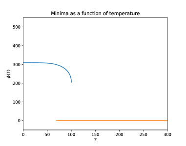
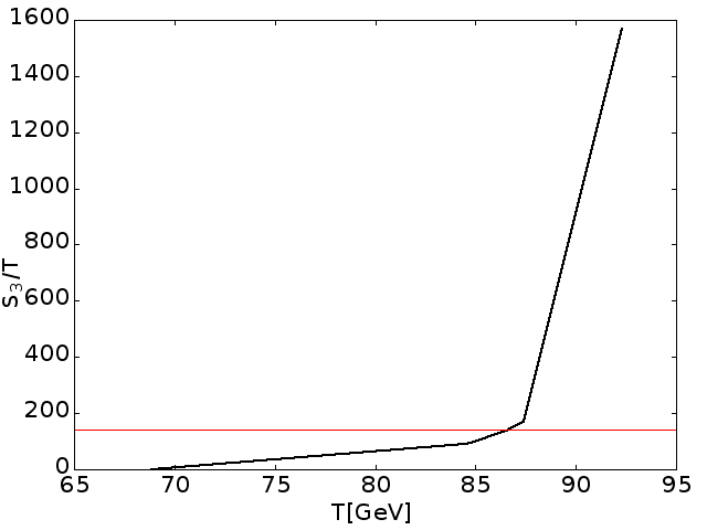
Figure 1: Variations of the phase transition properties with temperature for BP1. In (a) we show how the phase factor ($\phi(T)$) varies with the temperaure and it creates a potential separation at $T_{n}$ = 86.62 GeV. Figure 1(b) gives the variation of the parameter $S_{3}/T$ with $T$ and the red solid line indicates that nucleation occurs for the condition $S_{3}/T$ =140. See text for details.

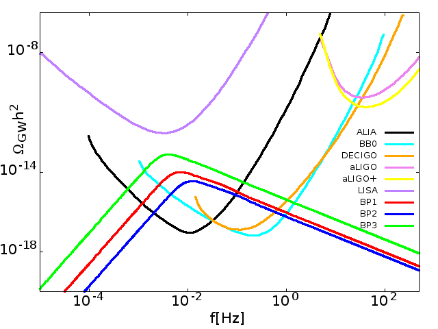
Figure 2: The variations of the GW intensity with frequency for each of the three BPs and their comparisons with the sensitivity curves of the detectors namely aLIGO, aLIGO+, ALIA, BBO, DECIGO and LISA. See text for details.

6 Summary and Conclusions

In this work, we have considered the emission of Gravitational Waves from first-order electroweak phase transitions involving a two component FIMP dark matter and the detectabilities of these Gravitational Waves by some proposed space based detectors in future. We consider a two component dark matter model where the scalar sector of Standard Model is extended by introducing two real scalars. The added scalars are singlets under SM gauge group SU(2)${}_{\rm L}\times$ U(1)_Y and constitute the two components of the present dark matter model. Both the components of this two component dark matter model are produced via “freeze-in” mechanism whereas their abundances grow from negligible amount towards the equilibrium value. These are Feebly Interacting Massive Particle or FIMP and in the present scenario their masses are within the range of few keV to few MeV. A discrete $Z_{2}\times Z^{\prime}_{2}$ symmetry is imposed on the two scalars to ensure their stability and they do not acquire any VEV at SSB. The extensive study of the dark matter phenomenology of the considered model as well as the theoretical and experimental constraints on the model parameters of the model have been discussed by one of the authors in a previous work [68]. We explore the possibility of first-order electroweak phase transition or EWPT with this model and subsequent productions of GWs. From the allowed parameter space we choose three benchmark points for both the analytical and numerical calculations of the GW intensity. Finite temperature corrections of the tree-level potential have been introduced for the calculations of the GW signals. For the model chosen parameters we compute the intensities of Gravitational Waves from the first-order EWPT initiated by the present extended SM. We compare our results with the projected sensitivities of future space based (ALIA, BBO, DECIGO amd LISA) as well as ground based (aLIGO and aLIGO+) GW detectors that would detect such primordial GWs. From our calculations it is observed that the peak values of such GWs lie within the detectable range of the future detectors such as ALIA, BBO and DECIGO. We also find that in the present dark matter model though the DM phenomenology (e.g. relic density calculations) can be addressed by considering very small Higgs portal couplings in FIMP mechanism, the production of the GW signals during the DM assisted EWPT is mostly governed by the couplings of the dark matter self interactions. Thus our two component FIMP dark matter model is in addition to a viable model for particle dark matter, it can cause GW productions via first-order electroweak phase transitions.

Acknowledgements: The authors would like to thank D. Majumdar for his useful comments and suggestions. The authors would also like to thank B. Banerjee for helping in the CosmoTransition package modification. One of the authors (MP) thanks the DST-INSPIRE fellowship grant (DST/INSPIRE/FELLOWSHIP/[IF160004]) by DST. Govt. of India.

References

- [1] B. P. Abbott et al. (LIGO Scientific, Virgo), Phys. Rev. Lett. 116, 061102 (2016).
- [2] A. A. Starobinsky, JETP Lett. 30, 682 (1979).
- [3] A. Vilenkin and E. P. S. Shellard, Cosmic Strings and Other Topological Defects, Cambridge University Press, 2000.
- [4] E. Witten, Phys. Rev. D 30, 272 (1984).
- [5] C. J. Hogan, Mon. Not. Roy. Astron. Soc. 218, 629 (1986).
- [6] J. Kozaczuk, S. Profumo, L. S. Haskins and C. L. Wainwright, JHEP 01, 144 (2015).
- [7] S. Profumo, M. J. Ramsey-Musolf, C. L. Wainwright and P. Winslow, Phys. Rev. D 91, 035018 (2015).
- [8] I. Baldes and C. Garcia-Cely, JHEP 05, 190 (2019).
- [9] D. Croon, V. Sanz and G. White, JHEP 08, 203 (2018).
- [10] P. Schwaller, Phys. Rev. Lett. 115, 181101 (2015).
- [11] V. Vaskonen, Phys. Rev. D 95, 123515 (2017).
- [12] W. Chao, H. K. Guo and J. Shu, JCAP 09, 009 (2017).
- [13] T. Hasegawa, N. Okada and O. Seto, Phys. Rev. D 99, 095039 (2019).
- [14] M. Artymowski, M. Lewicki and J. D. Wells, JHEP 03, 066 (2017).
- [15] P. S. B. Dev, F. Ferrer, Y. Zhang and Y. Zhang, arXiv:1905.00891 [hep-ph].
- [16] V. R. Shajiee and A. Tofighi, Eur. Phys. J. C 79, 360 (2019).
- [17] A. Mohamadnejad, arXiv:1907.08899 [hep-ph].
- [18] A. Mazumdar and G. White, Rept. Prog. Phys. 82, 076901 (2019).
- [19] F. P. Huang and J. H. Yu, Phys. Rev. D 98, 095022 (2018).
- [20] V. A. Kuzmin, V. A. Rubakov and M. E. Shaposhnikov, Phys. Lett. B 155, 36 (1985).
- [21] A. G. Cohen, D. B. Kaplan and A. E. Nelson, Ann. Rev. Nucl. Part. Sci. 43, 27 (1993).
- [22] A. Riotto and M. Trodden, Ann. Rev. Nucl. Part. Sci. 49, 35 (1999).
- [23] D. E. Morrissey and M. J. Ramsey-Musolf, New J. Phys. 14, 125003 (2012).
- [24] G. Gil, P. Chankowski, and M. Krawczyk, Phys. Lett. B 717, 396-402 (2012).
- [25] T. A. Chowdhury et al., JCAP 02, 029 (2012).
- [26] D. Borah and J. M. Cline, Phys. Rev. D 86, 055001 (2012).
- [27] J. M. Cline and K. Kainulainen, Phys. Rev. D 87, 071701 (2013).
- [28] S. S. AbduSalam and T. A. Chowdhury, JCAP 05, 026 (2014).
- [29] C. Cheung and Y. Zhang, JHEP 09, 002 (2013).
- [30] H. H. Patel and M. J. Ramsey-Musolf, Phys. Rev. D 33, 035013 (2013).
- [31] S. Inoue, G. Ovanesyan, and M. J. Ramsey-Musolf, Phys. Rev. D 93, 015013 (2013).
- [32] H. H. Patel, M. J. Ramsey-Musolf, and M. B. Wise, Phys. Rev. D 88, 015003 (2013).
- [33] M. Chala, G. Nardini, and I. Sobolev, Phys. Rev. D 94, 055006 (2016).
- [34] V. Vaskonen, arxiv:1611.02073 [hep-ph].
- [35] S. J. Huber et al., JCAP 03, 036 (2016).
- [36] D. Land and E. D. Carlson, Phys. Lett. B 292, 107-112 (1992).
- [37] W. Huang et al., Phys. Rev. D 91, 025006 (2015).
- [38] N. Blinov et al., Phys. Rev. D 92, 035012 (2015).
- [39] S. R. Coleman, Phys. Rev. D. 15, 2929-2936 (1977), [Erratum: Phys. Rev. D 16, 1248 (1977)
- [40] A. D. Linde, Nucl. Phys. B. 126, 421 (1983). [Erratum: Nucl. Phys. B 223, 544 (1983)
- [41] A. D. Linde, Phys. Lett. B 100, 37-40 (1981).
- [42] A. Kosowsky, M. S. Turner and R. Watkins, Phys. Rev. D 45, 4514 (1992).
- [43] A. Kosowsky and M. S. Turner, Phys. Rev. D 47, 4372 (1993).
- [44] S. J. Huber and T. Konstandin, JCAP 09, 022 (2008).
- [45] A. Kosowsky, M. S. Turner and R. Watkins, Phys. Rev. Lett. 69, 2026 (1992).
- [46] M. Kamionkowski, A. Kosowsky and M. S. Turner, Phys. Rev. D 49, 2837 (1994).
- [47] C. Caprini, R. Durrer and G. Servant, Phys. Rev. D 77, 124015 (2008). [astro-ph]].
- [48] M. Hindmarsh, S. J. Huber, K. Rummukainen and D. J. Weir, Phys. Rev. Lett. 112, 041301 (2014).
- [49] J. T. Giblin, Jr. and J. B. Mertens, JHEP 12, 042 (2013).
- [50] J. T. Giblin and J. B. Mertens, Phys. Rev. D 90, 023532 (2014).
- [51] M. Hindmarsh, S. J. Huber, K. Rummukainen and D. J. Weir, Phys. Rev. D 92, 123009 (2015).
- [52] C. Caprini and R. Durrer, Phys. Rev. D 74, 063521 (2006).
- [53] T. Kahniashvili, A. Kosowsky, G. Gogoberidze and Y. Maravin, Phys. Rev. D 78, 043003 (2008).
- [54] T. Kahniashvili, L. Campanelli, G. Gogoberidze, Y. Maravin and B. Ratra, Phys. Rev. D 78, 123006 (2008), Erratum: [Phys. Rev. D 79, 109901 (2009)].
- [55] T. Kahniashvili, L. Kisslinger and T. Stevens, Phys. Rev. D 81, 023004 (2010).
- [56] A. Paul, B. Banerjee and D. Majumdar, JCAP 10, 062 (2019).
- [57] B. Barman, A. D. Banik and A. Paul, arXiv:[1912.12899].
- [58] C. Caprini, R. Durrer and G. Servant, JCAP 12, 024 (2009).
- [59] C. E. Yaguna, JHEP 1108, 060 (2011).
- [60] E. Molinaro, C. E. Yaguna and O. Zapata, JCAP 1407, 015 (2014).
- [61] S. P. Zakeri et al., Chinese Physics C 42, 073101 (2018).
- [62] A.D. Banik et al., Eur. Phys. J. C 77, 657 (2017).
- [63] G. Jungman, M. Kamionkowski and K. Griest, Phys. Rept. 267, 195 (1996). [hep-ph/9506380].
- [64] A. Paul, D. Majumdar and A. Dutta Banik, JCAP 05, 029 (2019).
- [65] A. Dutta Banik, D. Majumdar and A. Biswas, Eur. Phys. J. C 76, 346 (2016).
- [66] A. Biswas, D. Majumdar and P. Roy, JHEP 1504, 065 (2015).
- [67] A. Biswas, D. Majumdar, A. Sil and P. Bhattacharjee, JCAP 1312, 049 (2013).
- [68] M. Pandey et al., JCAP 06, 023 (2018).
- [69] D. Harvey, R. Massey, T. Kitching, A. Taylor and E. Tittley, Science 347, 1462 (2015).
- [70] M. E. Shaposhnikov, JETP Lett. 44, 465-468 (1986).
- [71] M. E. Shaposhnikov, Nucl. Phys. B 287, 757-775 (1987).
- [72] J. M. Cline, “Baryogenesis”, in Les Houches Summer School- Session 86: Particle Physics and Cosmology: The Fabric of Spacetime Les Houches, France, July 31-August 25, 2006.
- [73] G. M. Harry, P. Fritschel, D. A. Shaddock, W. Folkner, and E. S. Phinney, Classical Quantum Gravity 23, 4887 (2006); 23, 7361(E) (2006).
- [74] C. Caprini et al., J. Cosmol. Astropart. Phys. 04, 001 (2016).
- [75] X. Gong et al., J. Phys. Conf. Ser. 610, 012011 (2015).
- [76] N. Seto, S. Kawamura, and T. Nakamura, Phys. Rev. Lett. 87, 221103 (2001).
- [77] Gregory M. Harry (LIGO Scientific Collaboration), Classical Quantum Gravity 27, 084006 (2010).
- [78] A. Dutta Banik and D. Majumdar, Phys. Lett. B 743, 420 (2015).
- [79] C. L. Wainwright, Comput. Phys. Commun. 183, 2006 (2012).
- [80] S. R. Coleman and E. J. Weinberg, Phys. Rev. D 7, 1888 (1973).
- [81] P. Basler, M. Krause, M. Muhlleitner, J. Wittbrodt and A. Wlotzka, JHEP 02, 121 (2017).
- [82] P. B. Arnold and O. Espinosa, Phys. Rev. D 47, 3546 (1993), Erratum: [Phys. Rev. D 50, 6662 (1994)].
- [83] A. D. Linde, Nucl. Phys. B 216, 421 (1983).
- [84] R. Jinno and M. Takimoto, Phys. Rev. D 95, 024009 (2017).
- [85] R. Jinno and M. Takimoto, JCAP 01, 060 (2019).
- [86] P. J. Steinhardt, Phys. Rev. D 25, 2074 (1982).
- [87] E. Madge and P. Schwaller, JHEP 02, 048 (2019).
- [88] M. Chala, V. V. Khoze, M. Spannowsky and P. Waite, arXiv:1905.00911 [hep-ph].
- [89] C. Caprini et al., JCAP 04, 001 (2016).
- [90] J. Ellis, M. Lewicki and J. M. No, JCAP 1904, 003 (2019).
- [91] J. Ellis, M. Lewicki, J. M. No and V. Vaskonen, JCAP 06, 024 (2019).
- [92] K. Kannike, Eur. Phys. J. C 72, 2093 (2012).
- [93] K.P. Modak, D. Majumdar and S. Rakshit, JCAP, 03 (2015) [arXiv:1312.7488v2[hep-ph]].
- [94] S. Bhattacharya, P. Ghosh and P. Poulose, JCAP 04, 043 (2017) [arXiv:1607.08461[hep-ph]].
- [95] S. Bhattacharya, P. Ghosh, T.N. Maity, T.S. Ray, [arXiv:1706.04699[hep-ph]].
- [96] G. Hinshaw et al. [WMAP Collaboration], Astrophys. J. Suppl. 208, 19 (2013).
- [97] B.W. Lee, C. Quigg and H.B. Thacker, Phys. Rev. D 16, 1519 (1977).
- [98] E. Thrane and J. D. Romano, Phys. Rev. D 88, 124032 (2013).
- [99] C. J. Moore, R. H. Cole, and C. P. L. Berry, Class. Quant. Grav. 32, 015014 (2015).
- [100] T. Alanne, T. Hugle, M. Platscher and K. Schmitz, JHEP 03, 004 (2020).
- [101] K. Schmitz, arXiv:2002.04615 [hep-ph].