Decentralized MCTS via Learned Teammate Models
Abstract
Decentralized online planning can be an attractive paradigm for cooperative multi-agent systems, due to improved scalability and robustness. A key difficulty of such approach lies in making accurate predictions about the decisions of other agents. In this paper, we present a trainable online decentralized planning algorithm based on decentralized Monte Carlo Tree Search, combined with models of teammates learned from previous episodic runs. By only allowing one agent to adapt its models at a time, under the assumption of ideal policy approximation, successive iterations of our method are guaranteed to improve joint policies, and eventually lead to convergence to a Nash equilibrium. We test the efficiency of the algorithm by performing experiments in several scenarios of the spatial task allocation environment introduced in Claes et al. (2015). We show that deep learning and convolutional neural networks can be employed to produce accurate policy approximators which exploit the spatial features of the problem, and that the proposed algorithm improves over the baseline planning performance for particularly challenging domain configurations.
1 Introduction
The ability to compute or learn plans to realize complex tasks is a central question in artificial intelligence. In the case of multi-agent systems, the coordination problem is of utmost importance: how can teams of artificial agents be engineered to work together, to achieve a common goal? A decentralized approach to this problem has been adopted in many techniques Durfee and Zilberstein (2013). The motivation comes from human collaboration: in most contexts we plan individually, and in parallel with other humans. Moreover, decentralized planning method can lead to a number of benefits, such as robustness, reduced computational load and absence of communication overhead Claes et al. (2017).
Decentralized planning methods were applied in context of multiplayer computer games Jaderberg et al. (2019), robot soccer Aşık and Akın (2012), intersection control Vu et al. (2018) and autonomous warehouse control Claes et al. (2017), to name a few. The essential difficulty of this paradigm lies in solving the coordination problem. To naively deploy single-agent algorithms for individual agents inevitably leads to the tragedy of the commons; i.e. a situation where an action that seems optimal from an individual perspective, is suboptimal collectively. For instance, consider a relatively simplistic instance of a spatial task allocation problem in which a team of robotic vacuum cleaners needs to clean a factory floor, as in Figure 1.
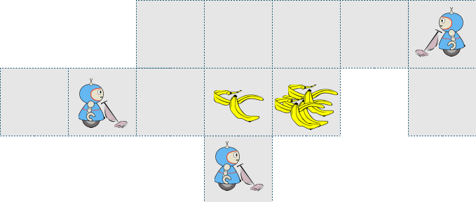
Assuming that a robot solves its own traveling salesman problem Lin (1965) would result in optimal path planning if it was alone in the factory; but collectively it could lead to unnecessary duplication of resources with multiple robots heading to the same littered area. On the other hand, joint optimization of all actions results in an intractable problem, that is not scalable to large networks of agents. Among some of the heuristic methods to deal with such problems proposed by researchers, communication Wu et al. (2009), higher level coordination orchestration Borrajo and Fernández (2019), and co-agent modelling Albrecht and Stone (2018) were previously explored in literature.
The cooperative decentralized planning problem can be posed in different settings; within this paper we focus on simulation-based planning, where each agent in the team has access to a simulator of the environment, which they can use to sample states and rewards, and evaluate the value of available actions, before committing to a particular one. The inherent difficulty of decentralized simulation-based planning is that in order for an individual agent to sample from the simulator and estimate the potential future rewards, it needs to provide joint actions of themselves and their teammates. However, in a live planning scenario, where each of the agents chooses actions according to their own simulation-based algorithm, it is not possible to know a priori what actions teammates actually execute.
There are two basic approaches to deal with this. If all agents are deployed with the same algorithm, they can evaluate all joint actions and choose their respective individual action; however this approach is costly, and the computational difficulty grows exponentially with the number of agents. A different approach is to make assumptions on other agents, and supply the simulator with an educated guess on their actions, given the common observed state. Such solution was used in Claes et al. (2017), where heuristic policies were designed for a domain modelling the task allocation problem in a factory floor.
In this paper, we build upon the second paradigm. We introduce a decentralized planning method of Alternate maximization with Behavioural Cloning (ABC). Our algorithm combines the ideas of alternate maximization, behavioral cloning and Monte Carlo Tree Search (MCTS) in a previously unexplored manner. By the ABC method, the agents learn the behavior of their teammates, and adapt to it in an iterative manner. The high-level overview of our planning-execution loop for a team of agents in a given environment can be represented in the following alternating steps:
-
1.
We perform a number of episode simulations with agents acting according to their individual MCTS; each agent has an own simulator of the environment and models of its teammates;
-
2.
The data from the simulations (in the form of state-action pairs for all agents) is used to train new agent behaviour models; these are in turn inserted into the MCTS simulator of one of the agents.
We refer to each successive iteration of above two steps as a generation. In each generation we chose a different agent for the simulator update.
We prove that if original policies have been perfectly replicated by learning, we are guaranteed to increase the mean total reward at each step, and eventually converge to a Nash equilibrium. We also demonstrate the empirical value of our method by experimental evaluation in the previously mentioned factory floor domain.
2 Related Work
In this paper, we take a so-called subjective perspective Oliehoek and Amato (2016) of the multi-agent scenario, in which the system is modeled from a protagonist agent’s view. The simplest approach simply ignores the other agents completely (some-times called ‘self-absorbed’ Claes et al. (2015)). On the complex end of the spectrum, there are ‘intentional model’ approaches that recursively model the other agents, such as the recursive modeling method Gmytrasiewicz and Durfee (1995), and interactive POMDPs Gmytrasiewicz and Doshi (2005); Doshi and Gmytrasiewicz (2009); Eck et al. (2019). In between lie other, often simpler, forms of modeling other agents Hernandez-Leal et al. (2017); Albrecht and Stone (2018); Hernandez-Leal et al. (2019). Such models can be tables, heuristics, finite-state machines, neural networks, other machine learning models, etc. Given that these do not explicitly model other agents, they have been called ‘sub-intentional’, however, as demonstrated by Rabinowitz et al. (2018) they can demonstrate complex characteristics associated with the ‘theory of mind’ Premack and Woodruff (1978).
In our approach we build on the idea that (sub-intentional) neural network models can indeed provide accurate models of behaviors of teammates. Contrary to Claes et al. (2017), who couple MCTS with heuristics to predict the teammates, this makes our method domain independent as well as providing certain guarantees (assuming ideal policy replication by function approximators). Recursive methods, such as the interactive particle filter Doshi and Gmytrasiewicz (2009) also give certain guarantees, but are typically based on a finite amount of recursion, which means that at the lowest level they make similar heuristic assumptions. Another drawback is their very high computational cost, making them very difficult to apply on-line.
In Kurzer et al. (2018) decentralized MCTS is combined with macro-actions for automated vehicle trajectory planning. The authors however assume heuristic (so not always accurate) models of other agents and do not learn their actual policies. Best et al. (2016) uses parallel MCTS for an active perception task and combines it with communication to solve the coordination problem; Li et al. (2019) explores similar ideas and combines communication with heuristic teammate models of Claes et al. (2017). Contrary to both of these papers, we assume no communication during the execution phase. Similarly, Golpayegani et al. (2015) uses MCTS in a parallel, decentralized way, but includes a so-called Collaborative Stage at each decision making point, where agents can jointly agree on the final decision. Other research has tried to make joint-action MCTS more scalable by exploiting factored state spaces Amato and Oliehoek (2015). In our setting, we do not make any assumptions about the dynamics of the environment.
Finally, we would like to point out similarity of our approach with AlphaGo & AlphaZero – the computer programs designed to master the game of Go in a highly acclaimed research by Deepmind Silver et al. (2016, 2017). There, neural network models were used together with self-play to guide MCTS, by providing guesses of opponents gameplay and estimates on state-action value functions. However, both AlphaGo & AlphaZero expand opponents’ actions in the search tree. By our approach, we are able to incorporate the actions of other agents in the environment simulator so they do not contribute to the branching factor of the decision tree, which, in turn, allows us to scale the method to several agents.
3 Background
A Markov Decision Process (MDP) is defined as a 5-tuple , where is a finite set of states, is a finite set of actions, are probabilities of transitioning between states for particular choices of actions, is a reward function and is the discount factor. The policy is a mapping , which represents an action selection rule for the agent. The policy is paired with the environment to form a Markov chain over the state space defined by the sequence of probability distribution functions which models the process of decision making. The value of a state is given by
| (1) |
One is typically interested in finding the optimal policy, . The value of action in a given state is given by the function
| (2) |
By the Bellman optimality principle, the actions with highest Q values form the optimal policy .
In a Multi-agent Markov Decision Process (MMDP) with agents the action space is factored in components: . Each component describes the individual actions available to the agent and the policies can be represented as products of individual agent policies . We emphasize that an MMDP is fully cooperative and all agents receive the same reward signal (contrary to e.g. stochastic games, where the rewards are individual). For our considerations, it will be useful to introduce the -th self-absorbed projection of an MMDP , after having fixed all individual policies besides , as a single agent MDP:
| (3) |
where denotes (fixed) policies of all agents except for agent and the transitions and the rewards are induced by compositions of with .
The problem of finding solutions to an MMDP can be viewed as a collaborative normal form game Claus and Boutilier (1998); Peshkin et al. (2000), where the agents are players, the individual policies are strategies, and the payoffs for a joint policy and an initial state are given by , and uniform to all players. A joint policy is a Nash equilibrium if and only if no higher payoff can be achieved by changing only one of the individual policies forming it. The optimal policy111For ease of exposition of the theoretical background, we assume it to be unique; this is not a restriction on the class of MDPs as one can always perturb the reward function in an otherwise negligible fashion to make policy values disjoint. is a Nash equilibrium, however there may be multiple other (suboptimal) Nash equilibria in the system.
The question of finding an optimal joint policy can be considered in the simulation-based planning context. There, it is no longer assumed that we have access to the full probabilistic model of the domain. Instead, one is supplied with a system simulator, i.e. a method for sampling new states and rewards based on states and joint actions , according to the underlying (but otherwise possibly unknown) probability distribution and reward function . In this paper, we consider the setting of online, decentralized, simulation-based planning, where the agents need to compute individual best responses over states they encounter in the episode.
We focus on one particularly effective and popular planning method: the MCTS algorithm combined with the Upper Confidence Trees (UCT) tree exploration policy. This search method uses Monte Carlo simulations to construct a tree of possible future evolutions of the system. The tree consists of nodes representing actions taken by the agent, and the resulting, sampled states encountered in the environment. Each node stores statistics that approximate either the state values or the values of actions. The single iteration of algorithm execution is split into four parts. First, the tree is traversed according to the tree policy (selection). Then, new nodes are created by sampling an action and the resulting state (expansion). Next, a heuristic policy is used to complete the episode simulation (rollout). Finally, the results are stored in the visited tree nodes (backpropagation).
The selection step is performed by choosing a node with an action , which maximizes the formula , where is a sample-based estimator of the value, is the amount of visits at the parent node of node , and is the amount of visits to the node. All of these three values are updated at each backpropagation step. The constant is the exploration constant; in theory, for rewards in range, it should be equal to . In practice the constant is chosen empirically Kocsis and Szepesvári (2006).
The algorithm is initialized and performed at each time step of simulation, for either a predefined, or time-limited amount of iterations. Then, the best action is selected greedily, based on the approximate -values of child nodes of the root node.
Definition 1.
We denote the policy generated by action selection according to the MCTS algorithm with UCT in an MDP by , with being the exploration constant, the number of UCT iterations and – a rollout policy.
For a sufficiently large number of iterations the MCTS algorithm approximates the real -values of each action node with arbitrary accuracy; and therefore it constitutes the pure, optimal policy: , c.f. Chang et al. (2005).
4 Alternating Maximization with Behavioral Cloning
In this section we describe the ABC algorithm and prove its convergence guarantees.
4.1 The Hill Climb
A common method for joint policy improvement in multi-agent decision making is the so-called hill climb, where agents alternate between improving their policies (c.f. Nair et al. (2003)). At each iteration of the method (i.e. generation), one of the agents is designated to compute its best response, while the other agents keep their policies fixed. The hill climb method comes with performance guarantees, in particular the joint rewards are guaranteed to (weakly) increase in subsequent generations.
Consider an MMDP on agents , and let denote the individual components of a joint policy .
Definition 2.
For each we define the -th best response operator from the joint policy space to itself by:
| (4) |
Lemma 1.
The following inequality holds:
| (5) |
Moreover, implies that is a fixed point of .
Proof.
For all :
| (6) | ||||
If the above are equal for all , then . ∎
Applications of Lemma 1 to simulation-based planning can seem counter-intuitive, and very much in spirit of the aphorism all models are wrong, but some are useful:
Remark 1.
Consider the following composition with for some joint policy ; the interpretation is that agent first adapts to the policies , including the -th agent’s policy ; then agent adapts to the policies . The subsequent application of on is likely to update agent ’s policy, which means that the assumption agent made to compute its best-response (namely that uses ) is no longer true. Nevertheless, as shown by Lemma 1, the value of the joint policy still increases.
Definition 3.
Let be a permutation on the set . We define the joint response operator by .
Corollary 1.
For all permutations and all initial joint policies the iterative application of operator converges to a Nash equilibrium. Since the policy space is finite, the convergence is achieved in finite time.
Proof.
To make the argument easier to follow, we will assume that , and denote as . For the purpose of this proof we denote the -th composition of by , for any . Since is non-decreasing as a function of joint policies, and the policy set is finite, for any joint policy there exists an such that . We will show that is a Nash equilibrium. Since increases along trajectories generated by , we have
| (7) |
Agent 1 has no incentive to deviate (c.f. the second part of Lemma 1), so
| (8) |
By an inductive argument
| (9) |
for all , which concludes the proof. ∎
4.2 Behavioral Cloning
In an online planning setting, accessing the policies of other agents can be computationally expensive, especially if the policies of individual agents are formed by executing an algorithm which evaluates the Q values “on-the-go” – such as in MCTS. To address this issue, we propose to use machine learning models.
More precisely, we divide our policy improvement process into generations; at each generation we update models in the simulator of one of our agents with samples of other agents’ policies from the previous generations. Through machine learning we are able to extrapolate and to give predictions of actions for states that were unseen during the previous simulation runs (i.e. were never explored by the policies of previous generations). By our method, each agent uses MCTS to conduct its own individual planning in the environment , where is a model of policies of other agents. Therefore, the planning is fully decentralized, and no communication is needed to execute the policies.
4.3 The ABC Pipeline
Our policy improvement pipeline based on MCTS is presented in pseudocode in Algorithm 1. The behavioral cloning algorithm is presented in pseudocode in Algorithm 2.
Inputs:
MMDP
initial heuristic policies
Parameters: number of generations
MCTS parameters ,
Outputs: improved policies
Start:
Inputs:
data of state-action pairs indexed by agents , in generation
neural network policy models , with softmax outputs over the action space
Outputs: trained policy models
Start:
Since MCTS with UCT converges to actual Q values, we can conclude that for sufficient number of UCT iterations our algorithm indeed executes the best responses to the assumed policies:
Corollary 2.
Let be as in Algorithm 1. For large enough , and as consequence .
If our machine learning model has enough data and degrees of freedom to perfectly replicate policies, from Lemma 1 and Corollary 1 we conclude that the procedure improves joint policies and eventually converges to a Nash equilibrium:
Theorem 1.
For large enough and under assumption , the joint policy value is non-decreasing as a function of , and strongly increasing until it reaches the Nash equilbrium. For large enough, is a Nash equilibrium.
We emphasize that it is essential that only one agent updates its assumed policies at each generation. If two or more agents would simultaneously update their policies, they could enter an infinite loop, always making the wrong assumptions about each other in each generation, and never achieving the Nash equilibrium.
We remark that in our algorithm we also leverage a learned model of agents’ own behavior by employing it in MCTS rollout stage.
5 Experiments
Our work is a natural extension to Claes et al. (2015, 2017), we perform experiments on a slightly modified version of the Factory Floor domain introduced therein. The baseline for our experiments is given by the current state of the art planning method for this domain: individual MCTS agents with heuristic models of other agents Claes et al. (2017), and it also serves as initialization (generation 0) of the ABC policy iterator. Therefore, the goal of the experiments is to empirically confirm the policy improvement via ABC. Any improvement over the 0th generation shows that we have managed to beat the baseline.
5.1 The Factory Floor Domain
The domain consists of a gridworld-like planar map, where each position can be occupied by (cleaning) robots and tasks (e.g. litter). Multiple robots and/or tasks can be in the same position. Each robot is controlled by an agent, and at each time step an agent can perform either a movement action , which shifts the position of the robot accordingly, or a cleaning action , which removes one task at the current position. Attempted actions may succeed or not, according to predefined probabilities. The reward collected at each time step is the number of tasks cleaned by the robots. At the beginning of the simulation there can already be some tasks on the map, and, as the simulation progresses, more tasks can appear, according to predefined probabilities.
5.2 Initial Heuristic Models
Below, we describe the heuristic policies , which are supplied as the model for MCTS agents in generation (the baseline). At each decision step, -th heuristic agent acts according to the following recipe:
-
1.
it computes the social order of the corresponding robot among all robots sharing the same position; the social ordering function is predefined by the lexicographic order of unique robot identifiers.
-
2.
It evaluates each possible destination by the following formula:
(10) -
3.
It assigns the -th best destination as the target destination, where is the computed social order of the corresponding robot (e.g. if it is the only robot at a given position, then ). Therefore, the social order is used to prevent several agents choosing the same destination.
-
4.
It chooses action if it is already at the target destination; and otherwise it selects a movement action along the shortest path to the destination.
5.3 MCTS Settings
We scale the exploration constant by the remaining time steps in the simulation, i.e. , to account for the decreasing range of possible future rewards, as recommended in Kocsis and Szepesvári (2006). As in the baseline, we also use sparse UCT Bjarnason et al. (2009) to combat the problem of a large state space; that means that we stop sampling child state nodes of a given action node from the simulator after we have sampled a given amount of times; instead we sample the next state node from the existing child state nodes, based on frequencies with which they occured. In all our experiments, we set this sampling limit to . As in the baseline, the agents are awarded an additional do-it-yourself bonus of in simulation, if they perform the task themselves; this incentivizes them to act, rather than rely on their teammates. Each agent performs 20000 iterations of UCT to choose the best action for their robot.
5.4 The Behavioral Cloning Model
Since the domain has spatial features, we opted to use a convolutional neural network as the machine learning method of choice for policy cloning.
As input we provide a 3-dimensional tensor with the width and the height equal to the width and the height of the Factory Floor domain grid, and with channels (i.e. the amount of robots plus two). We include the current time step information in the state. The -th channel layer is a matrix filled with integers representing the amount of tasks at a given position. The tasks have finite execution time, and the current time step affects the optimal decision choice; therefore we encode the current time step by filling it in the entries of the 1st channel. Finally, for , the -th channel is encoding the position of robot , by setting where the robot is positioned and on all other fields.
Such state representation is fed into the neural network with two convolutional layers of 2x2 convolutions followed by three fully connected layers with 64, 16 and 5 neurons respectively. We use the rectified linear unit activation functions between the layers, except for the activation of the last layer, which is given by the softmax activation function. The network has been trained using the categorical cross entropy function as the loss function, and Adam as the optimization method Kingma and Ba (2014). The action assigned to the state during MCTS simulations is corresponding to the argmax coordinate of the softmax probabilities. The time required to train the neural network is insignificant, compared to the time needed to collect data from MCTS simulations.
5.5 Domain Initialization
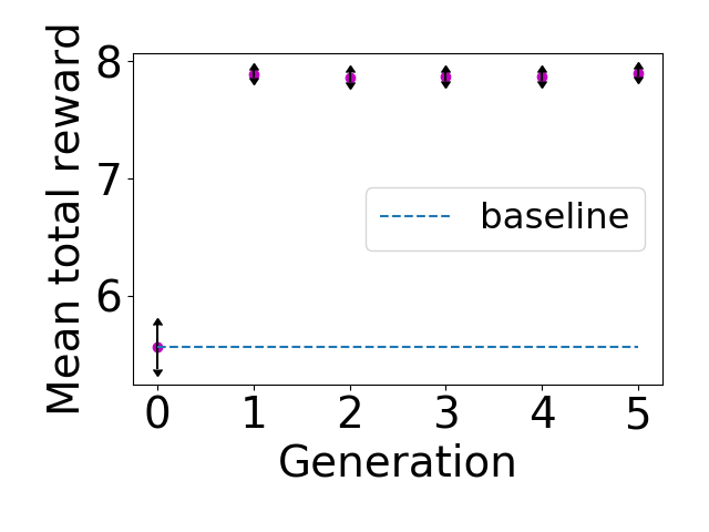
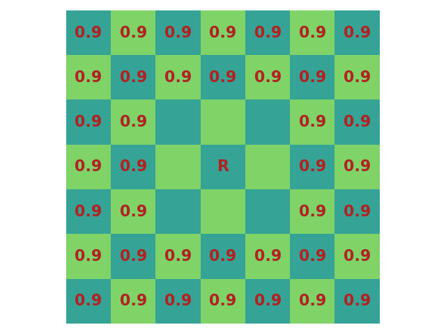
We tested our method in four experiments. In all experimental subdomains, the movement actions are assumed to succeed with probability , and the action is assumed to succeed always. In all configurations the horizon is set to ten steps, and the factor is set to , so there is no discounting of future rewards. We present the initial configuration of the experiment and the corresponding reward plots in Figures 2, 3, and 4. Letters indicate robot positions, and the numbers indicate the amount of tasks at a given position – for a fixed task placement; or the probability that a task appears at a given position – for dynamic task placement. We provide plots of the results, that contain the mean average reward for each generation, together with 95% confidence interval bars.
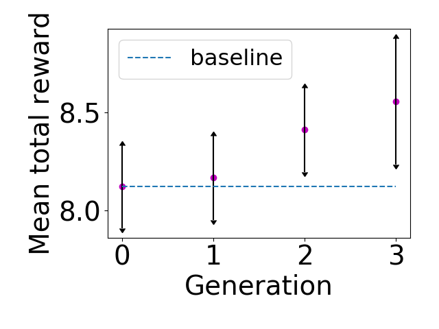
We chose domain configurations which, due to the location of tasks, require high level of coordination between agents. In particular, we created the domains where we expect that the policies of the baseline are suboptimal. For more generic domains, the decentralized MCTS with heuristic models is already close to optimal, and we do not expect much improvement. In subdomains with fixed positions of tasks we train the agents for five generations. In subdomains, where the tasks are assigned dynamically, we train the agents for three generations, as for higher amount of iterations we sometimes observed worsening performance, which we attribute to imperfect learning process due to high stochasticity of the domain.
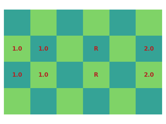
Two robots.
Our first subdomain is a trivial task: a 6x4 map, which has eight tasks to be collected. Even in such a simple scenario, the baseline does not perform well, because both robots make the assumption that their colleague will serve the task piles of ’s and head for the s, achieving a mean reward of (0th generation). The exploration parameter is set to , and the number of simulations at each generation to 320. Already in the first generation, agent learns the policy of agent and adapts accordingly, which results in an increase of the mean collected reward to . The average collected reward stabilizes through the next generations, which suggests that our method reached a Nash equilibrium (and in fact a global optimum, given that the maximal reward that could have been obtained in each episode is ).
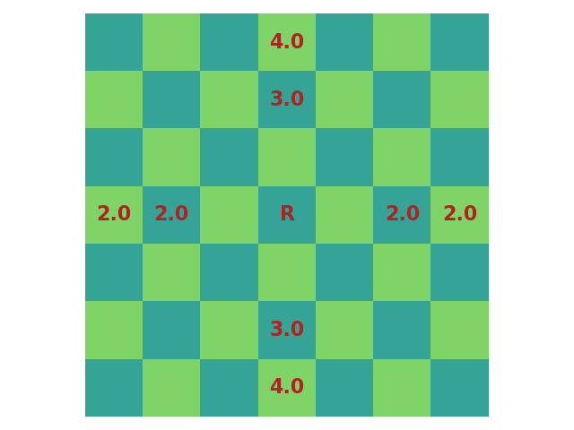
Four robots, fixed tasks.
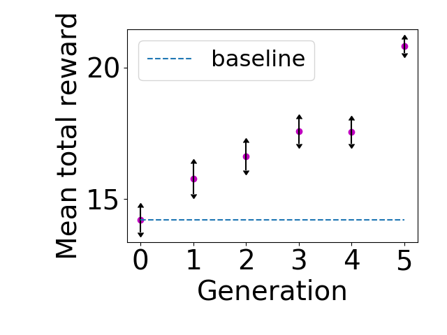
Our second subdomain is a 7x7 map which has 22 tasks to be collected by four robots. The exploration parameter is increased to – to account for higher possible rewards, and the number of simulations at each generation is decreased to – to account for longer simulation times. All robots start from the middle of the map. The baseline method again underpeforms, as the robots are incentivized to go for the task piles of 3’s and 4’s, instead of spreading in all four directions. After the application of the ABC algorithm the robots learn the directions of their teammates, spread, and a near optimal learning performance is achieved, see Figure 3.
Four robots, dynamic tasks.
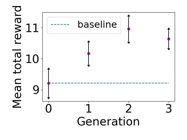
For the final two experiments we chose the same 7x7 map as previously, but this time tasks appear dynamically: two or three new tasks are added randomly with probability 0.9 at each time step during the program execution in one of the marked places. All the other experiment parameters remain unchanged. The confidence intervals are wider, due to additional randomness. Nevertheless, for the first three generations we observed an improvement over the 0th generation, which we attribute to the fact that the agents have learnt that they should spread to cover the task allocation region, similarly as in the experiment with fixed task location.
6 Conclusions
We have proposed a machine-learning-fueled method of improving teams of MCTS agents. Our method is grounded in the theory of alternating maximization and, given sufficiently rich training data and suitable planning time, it is guaranteed to improve the initial joint policies and reach a local Nash equilibrium. We have demonstrated in experiments, that the method allows to improve team policies for spatial task allocation domains, where coordination is crucial to achieve optimal results.
An interesting direction of future work is to search for the global optimum of the adaptation process, rather than a local Nash equilibrium. To that end, one can randomize the orded in which agents are adapting, find multiple Nash equilibria, and select the one with highest performance. Another research avenue is to extend the ABC method to environments with partial information (Dec-POMDPs), where the agents need to reason over the information set available to their teammates.
Acknowledgments
This project received funding from EPSRC First Grant EP/R001227/1, and the European Research Council (ERC) under the European Union’s Horizon 2020 research and innovation programme (grant agreement No. 758824 —INFLUENCE).
References
- Albrecht and Stone [2018] Stefano V Albrecht and Peter Stone. Autonomous agents modelling other agents: A comprehensive survey and open problems. Artificial Intelligence, 258:66–95, 2018.
- Amato and Oliehoek [2015] Christopher Amato and Frans A Oliehoek. Scalable planning and learning for multiagent pomdps. In Proceedings of the 29th AAAI Conference on Artificial Intelligence, 2015.
- Aşık and Akın [2012] Okan Aşık and H Levent Akın. Solving multi-agent decision problems modeled as Dec-POMPD: A robot soccer case study. In Robot Soccer World Cup, pages 130–140, 2012.
- Best et al. [2016] Graeme Best, O Cliff, Timothy Patten, Ramgopal Mettu, and Robert Fitch. Decentralised Monte Carlo tree search for active perception. In Workshop on the Algorithmic Foundations of Robotics, 2016.
- Bjarnason et al. [2009] Ronald Bjarnason, Alan Fern, and Prasad Tadepalli. Lower bounding Klondike solitaire with Monte-Carlo planning. In Nineteenth International Conference on Automated Planning and Scheduling, 2009.
- Borrajo and Fernández [2019] Daniel Borrajo and Susana Fernández. Efficient approaches for multi-agent planning. Knowledge and Information Systems, 58(2):425–479, 2019.
- Chang et al. [2005] Hyeong Soo Chang, Michael C Fu, Jiaqiao Hu, and Steven I Marcus. An adaptive sampling algorithm for solving Markov Decision Processes. Operations Research, 53(1):126–139, 2005.
- Claes et al. [2015] Daniel Claes, Philipp Robbel, Frans A. Oliehoek, Karl Tuyls, Daniel Hennes, and Wiebe Van der Hoek. Effective approximations for multi-robot coordination in spatially distributed tasks. In Proceedings of the 14th International Conference on Autonomous Agents and Multiagent Systems, pages 881–890, 2015.
- Claes et al. [2017] Daniel Claes, Frans Oliehoek, Hendrik Baier, and Karl Tuyls. Decentralised online planning for multi-robot warehouse commissioning. In Proceedings of the 16th International Conference on Autonomous Agents and Multiagent Systems, pages 492–500, 2017.
- Claus and Boutilier [1998] Caroline Claus and Craig Boutilier. The dynamics of reinforcement learning in cooperative multiagent systems. Proceedings of the 15th National/10th Conference on Artificial intelligence/Innovative Applications of Artificial Intelligence, 1998(746-752):2, 1998.
- Doshi and Gmytrasiewicz [2009] Prashant Doshi and Piotr J Gmytrasiewicz. Monte Carlo sampling methods for approximating interactive POMDPs. Journal of Artificial Intelligence Research, 34:297–337, 2009.
- Durfee and Zilberstein [2013] Edmund H Durfee and Shlomo Zilberstein. Multiagent planning, control, and execution. In Multiagent Systems, volume 11, pages 485–545. 2013.
- Eck et al. [2019] Adam Eck, Maulik Shah, Prashant Doshi, and Leen-Kiat Soh. Scalable decision-theoretic planning in open and typed multiagent systems. arXiv preprint arXiv:1911.08642, 2019. to appear in Proceedings of the 34th AAAI Conference on Artificial Intelligence.
- Gmytrasiewicz and Doshi [2005] Piotr J Gmytrasiewicz and Prashant Doshi. A framework for sequential planning in multi-agent settings. Journal of Artificial Intelligence Research, 24:49–79, 2005.
- Gmytrasiewicz and Durfee [1995] Piotr J. Gmytrasiewicz and Edmund H. Durfee. A rigorous, operational formalization of recursive modeling. In Proceedings of the 1st International Conference on Multiagent Systems, pages 125–132, 1995.
- Golpayegani et al. [2015] Fatemeh Golpayegani, Ivana Dusparic, and Siobhan Clarke. Collaborative, parallel Monte Carlo tree search for autonomous electricity demand management. In 2015 Sustainable Internet and ICT for Sustainability, pages 1–8, 2015.
- Hernandez-Leal et al. [2017] Pablo Hernandez-Leal, Michael Kaisers, Tim Baarslag, and Enrique Munoz de Cote. A Survey of Learning in Multiagent Environments: Dealing with Non-Stationarity. arXiv preprint arXiv:1707.09183, 2017.
- Hernandez-Leal et al. [2019] Pablo Hernandez-Leal, Bilal Kartal, and Matthew E Taylor. Agent modeling as auxiliary task for deep reinforcement learning. In Proceedings of the AAAI Conference on Artificial Intelligence and Interactive Digital Entertainment, pages 31–37, 2019.
- Jaderberg et al. [2019] Max Jaderberg, Wojciech M Czarnecki, Iain Dunning, Luke Marris, Guy Lever, Antonio Garcia Castaneda, Charles Beattie, Neil C Rabinowitz, Ari S Morcos, Avraham Ruderman, et al. Human-level performance in 3d multiplayer games with population-based reinforcement learning. Science, 364(6443):859–865, 2019.
- Kingma and Ba [2014] Diederik P Kingma and Jimmy Ba. Adam: A method for stochastic optimization. arXiv preprint arXiv:1412.6980, 2014.
- Kocsis and Szepesvári [2006] Levente Kocsis and Csaba Szepesvári. Bandit based Monte-Carlo planning. In European conference on machine learning, pages 282–293, 2006.
- Kurzer et al. [2018] Karl Kurzer, Chenyang Zhou, and J Marius Zöllner. Decentralized cooperative planning for automated vehicles with hierarchical Monte Carlo tree search. In IEEE Intelligent Vehicles Symposium, pages 529–536, 2018.
- Li et al. [2019] Minglong Li, Wenjing Yang, Zhongxuan Cai, Shaowu Yang, and Ji Wang. Integrating decision sharing with prediction in decentralized planning for multi-agent coordination under uncertainty. In Proceedings of the 28th International Joint Conference on Artificial Intelligence, pages 450–456, 2019.
- Lin [1965] Shen Lin. Computer solutions of the traveling salesman problem. Bell System Technical Journal, 44(10):2245–2269, 1965.
- Nair et al. [2003] Ranjit Nair, Milind Tambe, Makoto Yokoo, David Pynadath, and Stacy Marsella. Taming decentralized POMDPs: Towards efficient policy computation for multiagent settings. In Proceedings of the 18th International Joint Conference on Artificial Intelligence, volume 3, pages 705–711, 2003.
- Oliehoek and Amato [2016] Frans A. Oliehoek and Christopher Amato. A Concise Introduction to Decentralized POMDPs. 2016.
- Peshkin et al. [2000] Leonid Peshkin, Kee-Eung Kim, Nicolas Meuleau, and Leslie Pack Kaelbling. Learning to cooperate via policy search. In Proceedings of the Sixteenth conference on Uncertainty in artificial intelligence, pages 489–496, 2000.
- Premack and Woodruff [1978] David Premack and Guy Woodruff. Does the chimpanzee have a theory of mind? Behavioral and brain sciences, 1(4):515–526, 1978.
- Rabinowitz et al. [2018] Neil Rabinowitz, Frank Perbet, Francis Song, Chiyuan Zhang, S. M. Ali Eslami, and Matthew Botvinick. Machine theory of mind. In Proceedings of the International Conference on Machine Learning, pages 4218–4227, July 2018.
- Silver et al. [2016] David Silver, Aja Huang, Chris J Maddison, Arthur Guez, Laurent Sifre, George Van Den Driessche, Julian Schrittwieser, Ioannis Antonoglou, Veda Panneershelvam, Marc Lanctot, et al. Mastering the game of Go with deep neural networks and tree search. Nature, 529(7587):484, 2016.
- Silver et al. [2017] David Silver, Julian Schrittwieser, Karen Simonyan, Ioannis Antonoglou, Aja Huang, Arthur Guez, Thomas Hubert, Lucas Baker, Matthew Lai, Adrian Bolton, et al. Mastering the game of go without human knowledge. Nature, 550(7676):354–359, 2017.
- Vu et al. [2018] Huan Vu, Samir Aknine, and Sarvapali D Ramchurn. A decentralised approach to intersection traffic management. In Proceedings of the 27th International Joint Conference on Artificial Intelligence, pages 527–533, 2018.
- Wu et al. [2009] Feng Wu, Shlomo Zilberstein, and Xiaoping Chen. Multi-agent online planning with communication. In Nineteenth International Conference on Automated Planning and Scheduling, 2009.