On the Analysis of Parallel Real-Time Tasks with Spin Locks

Abstract

Locking protocol is an essential component in resource management of real-time systems, which coordinates mutually exclusive accesses to shared resources from different tasks. Although the design and analysis of locking protocols have been intensively studied for sequential real-time tasks, there has been little work on this topic for parallel real-time tasks. In this paper, we study the analysis of parallel real-time tasks using spin locks to protect accesses to shared resources in three commonly used request serving orders (unordered, FIFO-order and priority-order). A remarkable feature making our analysis method more accurate is to systematically analyze the blocking time which may delay a task’s finishing time, where the impact to the total workload and the longest path length is jointly considered, rather than analyzing them separately and counting all blocking time as the workload that delays a task’s finishing time, as commonly assumed in the state-of-the-art.

1 Introduction

Real-time systems are playing a more important role in our daily life as computing is closely integrated to the physical world. Violating timing constraints in such systems may lead to catastrophic consequences such as loss of human life. Therefore, real-time systems must manage resource in a way such that timing correctness can be guaranteed. Locking protocol is an essential component in resource management of real-time systems, which coordinates mutually exclusive accesses to shared physical/logical resources by different tasks. Inappropriate design or incorrect analysis of locking protocols will lead to incorrect system timing behavior, e.g., as in the famous software failure accident in Mars Pathfinder [1].

Multi-cores are becoming mainstream hardware platforms for real-time systems, to meet their rapidly increasing requirements in high performance and low power consumption. To fully utilize the processing capacity of multi-cores, software should be parallelized. While locking protocols for sequential real-time task systems have been intensively studied in classical real-time scheduling theory [2, 3, 4, 5], there is little work on this topic for parallel real-time tasks. On the other hand, there has been much work on scheduling algorithms and analysis techniques for parallel real time tasks [6, 7, 8], where tasks are assumed to be independent from each other and the locking issue is not considered.

Recently, spin locks were studied for parallel real-time tasks in [9] where each parallel task is scheduled exclusively on several pre-assigned processors (i.e., by the federated scheduling approach [6]). However, the analysis in [9] is pessimistic. The contribution of our work is to develop new techniques for the schedulability analysis of real-time parallel tasks with spin locks and significantly improve the analysis precision against the state-of-the-art.

Both [9] and our work only require knowledge of the total worst-case execution time (WCET) $\mathcal{C}_{i}$ and longest path length $\mathcal{L}_{i}$ of each task, but not the exact graph structure (the benefits of only using the abstract $\mathcal{C}_{i}$ and $\mathcal{L}_{i}$ information in the analysis will be discussed in Section 2.4). In [9]’s analysis, all blocking time caused by spin locks is considered to contribute to the workload that delays the finishing time of a parallel task, which is added to $\mathcal{C}_{i}$ and $\mathcal{L}_{i}$ in their worst-case scenarios separately. This is quite pessimistic since many blocking time can not delay the finishing time of a parallel task due to the parallelism and intra-dependencies. Moreover, the worst-case scenario leading to the maximal increase to $\mathcal{C}_{i}$ is in general different from the worst-case scenario leading to the maximal increase to $\mathcal{L}_{i}$.

To solve these problems, in this work we first develop new schedulability analysis techniques for parallel tasks with spin locks, where the blocking time contributing to the workload that may delay a task’s finishing time is systematically defined and analyzed. Further, we develop blocking analysis techniques for three common request serving orders, i.e., unordered, FIFO-order and priority-order, where the impact to $\mathcal{C}_{i}$ and $\mathcal{L}_{i}$ is jointly considered thus achieving higher analysis precision.

We conduct experiments to evaluate the precision improvement using our new techniques compared with [9], with both randomly generated tasks and workload generated according to realistic OpenMP programs. Experimental results show that our techniques consistently outperform [9] under different settings.

2 Preliminary

2.1 Task Model

We consider a task set $\mathcal{T}$ consisting of several periodic DAG tasks $\mathcal{T}=\{\tau_{1},\tau_{2},...,\tau_{|\mathcal{T}|}\}$ to be executed on $m$ processors. A task $\tau_{i}$ has a period $T_{i}$, a relative deadline $D_{i}$ and a workload structure modeled by a Directed Acyclic Graph (DAG) $G_{i}=\langle V_{i},E_{i}\rangle$, where $V_{i}$ is the set of vertices and $E_{i}$ is the set of edges in $G_{i}$. Tasks have constrained deadlines, i.e., $D_{i}\leq T_{i}$. Each vertex $v\in V_{i}$ is characterized by a worst-case execution time (WCET) $c(v)$. We use $\mathcal{C}_{i}$ to denote the total WCET of all vertices of $\tau_{i}$: $\mathcal{C}_{i}=\sum_{v\in V_{i}}c(v)$. The utilization of task $\tau_{i}$ is $U_{i}=\mathcal{C}_{i}/T_{i}$ and the density of task $\tau_{i}$ is $\Gamma_{i}=\mathcal{C}_{i}/D_{i}$. In this paper, we only consider DAG tasks with $\Gamma_{i}>1$, as those with $\Gamma_{i}\leq 1$ can be executed sequentially and handled by existing techniques for sequential real-time tasks.

Each edge $(u,v)\in E_{i}$ represents the precedence relation between vertices $u$ and $v$, where $u$ is a predecessor of $v$, and $v$ is a successor of $u$. We assume each DAG has a unique head vertex (with no predecessors) and a unique tail vertex (with no successors). This assumption does not limit the expressiveness of our model since one can always add a dummy head/tail vertex to a DAG having multiple entry/exit points. A complete path in a DAG task is a sequence of vertices $\pi=\{v_{1},v_{2},...,v_{p}\}$, where the first element $v_{1}$ is the head vertex of $G_{i}$, the last element $v_{p}$ is the tail vertex of $G_{i}$, and $v_{j}$ is a predecessor of $v_{j+1}$ for each pair of consecutive elements $v_{j}$ and $v_{j+1}$ in $\pi$. The length of each path $\pi$ is $len(\pi)=\sum_{v\in\pi}c(v)$. We use $\mathcal{L}_{i}$ to denote the longest length among all paths in $G_{i}$: $\mathcal{L}_{i}=\max_{\pi\in G_{i}}\{len(\pi)\}$. Task $\tau_{i}$ generates a potentially infinite sequence of jobs, which inherit $\tau_{i}$’s DAG workload structure $G_{i}$. Let $J$ be a job released by $\tau_{i}$, then we use $r(J)$ to denote $J$’s release time and $f(J)$ to denote $J$’s finish time. The absolute deadline of $J$ is calculated by $r(J)+D_{i}$. At runtime, we say a vertex (of a job $J$) is eligible at some time point if all its predecessors (of the same job $J$) have been finished and thus it can immediately execute if there are available processors. Fig. 1 shows a DAG task example $\tau_{i}$ with $7$ vertices, where $\mathcal{C}_{i}=10$ and $\mathcal{L}_{i}=5$ (the longest path is $\{v_{1},v_{4},v_{6},v_{7}\}$ or $\{v_{1},v_{2},v_{6},v_{7}\}$).

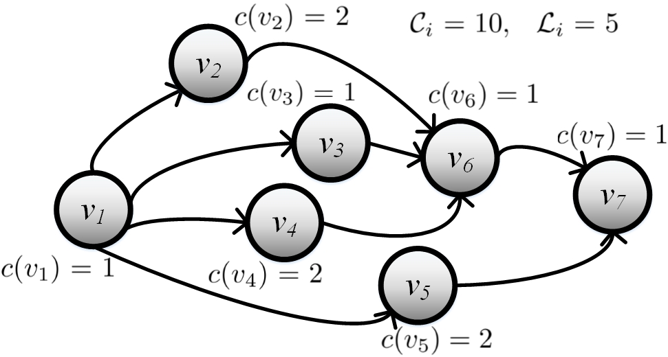
Figure 1: An example of a DAG task $\tau_{i}$.

2.2 Resource and Lock Model

There is a limited set of serially-reusable shared resources (called resources for short) $\Theta=\{\ell_{1},\ell_{2},...,\ell_{|\Theta|}\}$ in the system, such as I/O ports, network links, message buffers, or other shared data structures. Resources are protected by spin locks, i.e., the program must acquire, hold and release the lock affiliated to $\ell_{q}$ before, during and after executing the code segment accessing $\ell_{q}$. We assume the code segment wrapped by a pair of lock acquisition and lock release does not cross different vertices. A vertex must execute non-preemptively when it is holding a lock. When a vertex acquires a lock affiliated to $\ell_{q}$ being held by other vertices (either from the same task or from other tasks), the acquiring vertex must spin non-preemptively until it successfully obtains the lock, and we say this vertex is spinning for $\ell_{q}$.

When multiple vertices are spinning for the same resource at the same time, we consider three kinds of order in which their requests will be served: unordered, FIFO-order and priority-order. In priority-order, each task is assigned a unique priority and all requests from vertices of a same task have the same priority. Note that the priorities are only used to decide the order when requests from different tasks to a resource are served.

A vertex may access different shared resources and thus hold different locks. However, we assume the locks are non-nested, i.e., a vertex never acquires another lock when holding a lock. We use $\Theta_{i}$ to denote the set of resources accessed by vertices of task $\tau_{i}$.

The worst-case time of each single access to $\ell_{q}$ by task $\tau_{i}$ (i.e., the maximal duration for a vertex in $\tau_{i}$ to hold the lock affiliated to $\ell_{q}$ once) is denoted by $L_{i,q}$, and the worst-case number of accesses to $\ell_{q}$ by $\tau_{i}$ is denoted by $N_{i,q}$. Note that a vertex’s WCET includes the resource access time. On the contrary, the time spent by a vertex on spinning for some resource, called blocking time [10, 11], is not included in the WCET estimation.

TABLE I: Notations adopted in this paper.

Notations	Descriptions
$\tau_{i}$	a DAG task
$G_{i}$	the workload structure of $\tau_{i}$
$V_{i}$	the set of vertices in $G_{i}$
$E_{i}$	the set of edges of $G_{i}$
$c(v)$	WCET of a vertex $v$
$\mathcal{C}_{i}$	total WCET of all vertices of $\tau_{i}$
$\pi$	a path
$\lambda$	a key path
$len(\pi)$	the total WCET of all vertices on $\pi$
$\mathcal{L}_{i}$	the longest length among all path of $\tau_{i}$
$\ell_{q}$	a shared resource
$N_{i,q}$	number of accesses to $\ell_{q}$ from $\tau_{i}$
$L_{i,q}$	the worst-case time of each single access to $\ell_{q}$ by $\tau_{i}$
$W_{i}$	working time of a job of $\tau_{i}$
$\Gamma_{i}$	idle time of a job of $\tau_{i}$
$B_{i}$	blocking time of a job of $\tau_{i}$
$B_{i}^{\lambda,I}$	intra-task key path blocking time of a job of $\tau_{i}$
$B_{i}^{\lambda,O}$	inter-task key path blocking time of a job of $\tau_{i}$
$B_{i}^{\overline{\lambda},I}$	intra-task delay blocking time of a job of $\tau_{i}$
$B_{i}^{\overline{\lambda},O}$	inter-task delay blocking time of a job of $\tau_{i}$
$B_{i}^{\widetilde{\lambda},I}$	intra-task parallel blocking time of a job of $\tau_{i}$
$B_{i}^{\widetilde{\lambda},O}$	inter-task parallel blocking time of a job of $\tau_{i}$
$\mathcal{I}_{i}$	defined in Lemma 3
$\mathcal{I}_{i,q}^{I}$	defined in (6)
$\mathcal{I}_{i,q}^{O}$	defined in (7)
$\eta_{i,j}^{q}$	defined in (11)
$\varDelta_{i,j}^{q}$	defined in (18)
$R_{i}$	worst-case response time of $\tau_{i}$

2.3 Scheduling Model

There are in total $m$ processors in the system, which will be partitioned into several subsets and each subset is assigned to a task. We use $m_{i}$ to denote the number of processors assigned to task $\tau_{i}$. At runtime, $\tau_{i}$ is scheduled by a work-conserving scheduling algorithm [6] exclusively on these $m_{i}$ processors. Note that although a task $\tau_{i}$ executes exclusively on its own $m_{i}$ processors, its timing behavior is still interfered by other tasks due to the contention on the shared resources. The response time $R(J)$ of a job $J$ is $R(J)=f(J)-r(J)$, and the worst-case response time (WCRT) $R_{i}$ of task $\tau_{i}$ is the maximum $R(J)$ among all its released jobs $J$. Task $\tau_{i}$ is schedulable if $R_{i}\leq D_{i}$. The problem to solve in this paper is how to partition the $m$ processors to each task such that it is guaranteed to be schedulable.

2.4 Remark

The analysis techniques of this paper only require the knowledge of $\mathcal{C}_{i}$ and $\mathcal{L}_{i}$ of each task $\tau_{i}$, as well as $N_{i,q}$ and $L_{i,q}$ for each pair of task $\tau_{i}$ and resource $\ell_{q}$. It is not required to know the exact graph structure of the task, neither the exact distribution of the resource access requests within the task. This makes our analysis techniques general, in the sense that they are directly applicable to more expressive models, e.g., the conditional DAG model, as long as we still can obtain the $\mathcal{C}_{i}$, $\mathcal{L}_{i}$, $N_{i,q}$, $L_{i,q}$ information. Moreover, as pointed out by [9], parallel programs are often data-dependent and their internal graph structures usually can only be unfolded at run time, so the exact graph structure of a parallel task can vary from one release to the next. Therefore, the analysis techniques using abstract information are more practical than those relying on exact graph structure information.

Of course if one can model the resource access behavior in a more detailed manner, e.g., giving the exact worst-case duration of each access and the information about which resource is accessed by which part of the task at which time point, it will certainly lead to more precise results in general. However, in practice it is not always possible to model realistic systems with those detailed information due to the flexibility and non-determinism of software behavior. Study on finer-grained resource access models and the corresponding analysis techniques is left as our future work.

It is necessary to mention that the main scope of this paper is to present blocking and schedulability analysis techniques when scheduling DAG tasks with spin locks. We do not make any constraint to the scheduler that each paralleled program is scheduled with, as long as the work-conserving is satisfied (e.g., EDF). A limitation in this paper is that we assume locks to be non-nested. In fact, the analysis of nested locks is more complicated even for sequential tasks, and this problem is still vastly open [12]. However, when nested-locks are used in practice, we can adopt some techniques such as group locks [12] to transform nested-locks into independent locks such that techniques presented in this paper are still applicable.

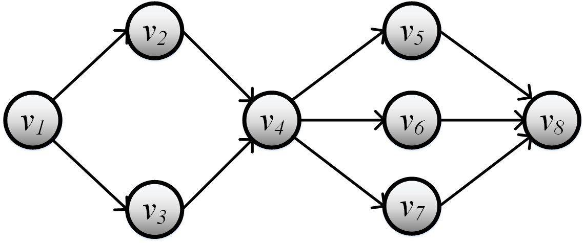
(a) An example of a DAG task.

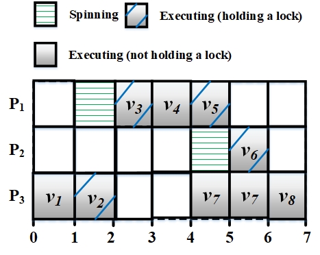
(b) A possible sequence.

Figure 2: An example of blocking behavior of a DAG job.

3 Discussion of existing techniques

There has been significant work of locking protocols and blocking analysis for sequential tasks (see Section 7 for more details). However, it is not a proper choice to directly apply blocking analysis techniques for sequential tasks on DAG tasks.

First, the definition of blocking for DAG tasks is different than that under sequential tasks. Under sequential task models, the blocking time of each task is analyzed individually, and the exact definition of blocking time as well as the blocking analysis techniques are developed according to some particular schedulability tests [10, 4, 13] where the blocking time can be accounted in. The main object of locking protocols (with blocking analysis) is to bound such maximum blocking (e.g., the priority inversion blocking [12, 13]) to an individual task. However, this is not the case for DAG tasks where the schedulability analysis object is the whole DAG task. For example, the DAG task in Figure 2.(a) has 8 vertices where $c(v_{7})=2$ and each of other vertices has a WCET of 1. $v_{2}$, $v_{3}$, $v_{5}$ and $v_{6}$ need to access a same shared resource $\ell_{q}$ for 1 time unit, while the remaining vertices do not need to access any share resource. A possible execution sequence of a job of $\tau_{i}$ is shown in Figure 2.(b) where $P_{1}$, $P_{2}$ and $P_{3}$ denote the processors. It can be observed that $v_{2}$ can not be blocked by $v_{3}$ if $v_{2}$ blocks $v_{3}$ in a DAG job (which is also the case for sequential tasks but each vertex must be analyzed individually in a worst-case blocking scenario). Moreover, although $v_{6}$ is blocked by $v_{5}$, the finishing time of the DAG job is not delayed. The reason is that the impact of blocking time on the schedualbility of a DAG job is actually reflected by its impact on the progress of a particular path, i.e., $\{v_{1},v_{3},v_{4},v_{7},v_{8}\}$ in Figure 2.(b). These are quite different than that under sequential task models where the blocking time of each task is analyzed individually. To develop blocking analysis for DAG tasks, we first need to systematically define the notion of blocking and analyze which blocking should be accounted according to its influence on the timing behavior of a DAG task.

Second, as discussed in Section 2.4, the exact distribution of resource access requests is not known under the model considered in this paper. Therefore, it is impossible to directly apply blocking analysis techniques for sequential tasks on the task model considered in this paper. There may also be cases where the exact graph structure and more concrete information about the resource access. In this case, one may utilize such concrete information and use sequential locking protocols to perform blocking analysis. We will evaluate the performance when directly applying OMLP and its associated blocking analysis techniques on DAG tasks in Section 6 to validate the problems discussed in this section.

4 Preparation

In this section, we introduce some useful concepts and present schedulability analysis techniques for parallel tasks that are applicable irrelevant of the locking protocols and request serving orders. Then in the next section we will apply these results to develop specific blocking analysis techniques for unordered, FIFO- and priority- request serving orders, respectively.

When we say a vertex is executing, it may be either holding or not holding a lock. We say a processor is busy if some vertex is executing or spinning on this processor, and say a processor is busy with a vertex $v$ if vertex $v$ is executing or spinning on this processor. A processor is said to be idle if it is not busy.

Let $J_{i}$ denote an arbitrary job of $\tau_{i}$, which is released at $r(J_{i})$ and finished at $f(J_{i})$. The total amount of time spent on $m_{i}$ processors assigned to $\tau_{i}$ during $[r(J_{i}),f(J_{i}))$ is $m_{i}\cdot(f(J_{i})-r(J_{i}))$, which can be divided into three disjoint parts $m_{i}\cdot(f(J_{i})-r(J_{i}))=B_{i}+W_{i}+\Gamma_{i}$:

• Blocking Time $B_{i}$: the cumulative length of time on $m_{i}$ processors spent on spinning.

• Working Time $W_{i}$: the cumulative length of time on $m_{i}$ processors spent on executing workload of $J_{i}$ (either holding a lock or not).

• Idle Time $\Gamma_{i}$: the cumulative length of time on $m_{i}$ processors being idle.

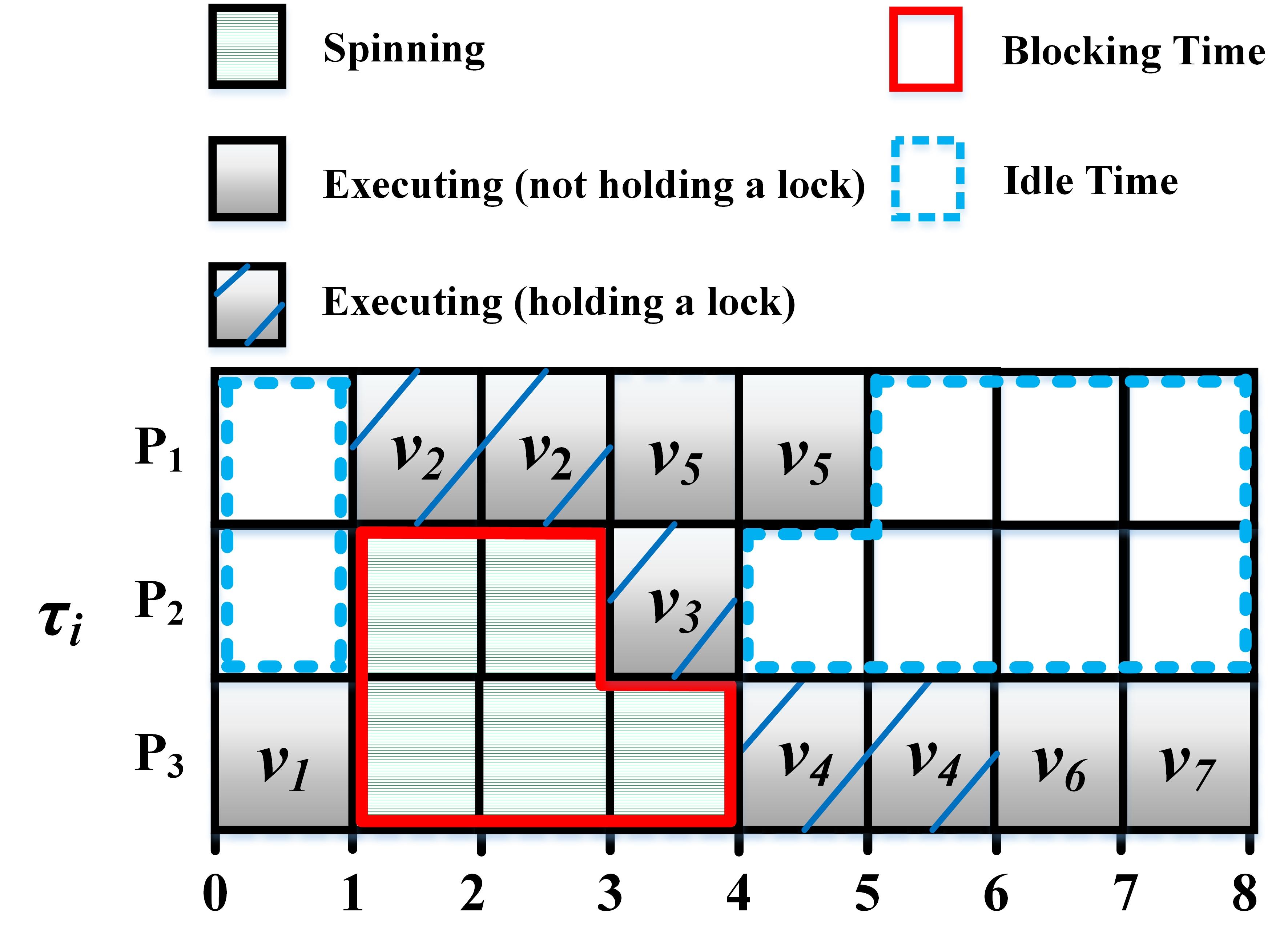
Figure 3: Illustration of different times.

Fig. 3 shows a possible scheduling sequence of a job of the task in Fig. 1 on $3$ processors, with release time $0$ and finish time $8$. Suppose that $v_{2}$, $v_{3}$, $v_{4}$ need to access the same shared resource $\ell_{q}$ for 1 time unit, while the remaining vertices do not need to access any share resource. The blocking time is $5$ (the area wrapped by red solid lines), the idle time is $9$ (the area wrapped by blue dash lines), and the working time is $10$ (the remaining area between $[0,8)$ on all the $3$ processors).

Given $m_{i}$ processors assigned to task $\tau_{i}$, we have:

Lemma 1.

$\tau_{i}$’s worst-case response time $R_{i}$ is bounded by:

$$R_{i}\leq\frac{B_{i}+\Gamma_{i}+\mathcal{C}_{i}}{m_{i}}.$$ (1)

Proof.

The response time of $J_{i}$ is $f(J_{i})-r(J_{i})$. By $m_{i}\cdot(f(J_{i})-r(J_{i}))=B_{i}+W_{i}+\Gamma_{i}$ and $W_{i}\leq\mathcal{C}_{i}$, we know $J_{i}$’s response time is bounded by $\frac{B_{i}+\mathcal{C}_{i}+\Gamma_{i}}{m_{i}}$. Since $J_{i}$ is an arbitrary job of $\tau_{i}$, $R_{i}$ is also bounded by $\frac{B_{i}+\mathcal{C}_{i}+\Gamma_{i}}{m_{i}}$. ∎

By Lemma 1, the problem of bounding $R_{i}$ boils down to bounding $B_{i}+\Gamma_{i}$. Before going further into the analysis, we first introduce the concept of key path:

Definition 1 (Key Path).

A key path of job $J_{i}$, denoted by $\lambda=\{v_{1},v_{2},...v_{p}\}$, is a complete path in $G_{i}$, s.t., $\forall j:1<j\leq p$, $v_{j-1}$ is a predecessor of $v_{j}$ with the latest finish time among all predecessors of $v_{j}$.

Lemma 2.

Let $\lambda=\{v_{1},v_{2},...v_{p}\}$ be a key path of $J_{i}$. All $m_{i}$ processors must be busy at any time point in $[r(J_{i}),f(J_{i}))$ when no processor is busy with vertices in $\lambda$.

Proof.

Let $v_{j}$ and $v_{j+1}$ be two successive elements in $\lambda$. By Definition 1, all predecessors of $v_{j+1}$ have finished at the finish time of $v_{j}$ (and thus $v_{j+1}$ is eligible for execution at that time point). Therefore, all processors must be busy between the finish time of $v_{j}$ and the starting time of $v_{j+1}$. Applying the above reasoning to each pair of successive elements in $\lambda$, the lemma is proved. ∎

In the following, we divide the blocking time $B_{i}$ into several disjoint parts. There are two dimensions to divide $B_{i}$. First, we can divide $B_{i}$ into:

• Key Path Blocking Time $B_{i}^{{\lambda}}$, the cumulative length of time spent on spinning by a vertex in $\lambda$.

• Delay Blocking Time $B_{i}^{\overline{\lambda}}$, the cumulative length of time on all $m_{i}$ processors spent on spinning during all the subintervals in $[r(J_{i}),f(J_{i}))$ when no processor is busy with a vertex in $\lambda$.

• Parallel Blocking Time $B_{i}^{\widetilde{\lambda}}$, the cumulative length of time on all other $m_{i}-1$ processors spent on spinning during all the subintervals in $[r(J_{i}),f(J_{i}))$ when one processor is busy with a vertex in $\lambda$.

In the second dimension we divide $B_{i}$ according to whether the processor is waiting for a resource locked by the same task or by a different task:

• Intra-task Blocking Time, the cumulative length of time spent on spinning and waiting for a resource locked by the same task,

• Inter-task Blocking Time, the cumulative length of time spent on spinning and waiting for a resource locked by other tasks,

so each of $B_{i}^{{\lambda}}$, $B_{i}^{\overline{\lambda}}$ and $B_{i}^{\widetilde{\lambda}}$ can be further divided into:

$$B_{i}^{{\lambda}}=B_{i}^{{\lambda},I}+B_{i}^{{\lambda},O};~{}B_{i}^{\overline{\lambda}}=B_{i}^{\overline{\lambda},I}+B_{i}^{\overline{\lambda},O};~{}B_{i}^{\widetilde{\lambda}}=B_{i}^{\widetilde{\lambda},I}+B_{i}^{\widetilde{\lambda},O}$$

where the superscript $I$ denotes intra-task blocking time and $O$ denotes inter-task blocking time. Finally, $B_{i}$ can be divided into the following six disjoint parts:

$$B_{i}=B_{i}^{\lambda,I}+B_{i}^{\lambda,O}+B_{i}^{\overline{\lambda},I}+B_{i}^{\overline{\lambda},O}+B_{i}^{\widetilde{\lambda},I}+B_{i}^{\widetilde{\lambda},O}.$$ (2)

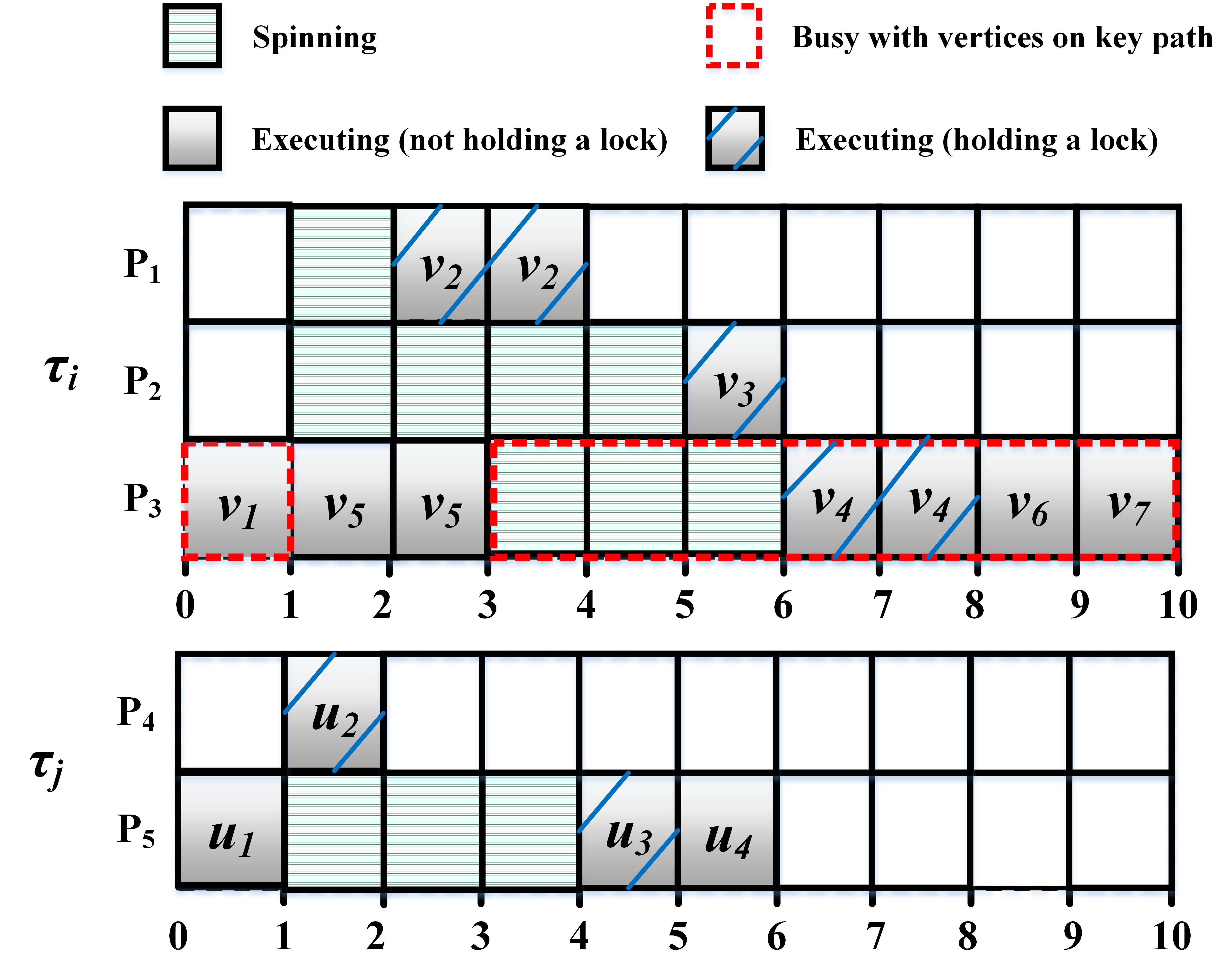
Figure 4: An example of blocking time.

We use the example in Fig. 4 to demonstrate different types of blocking time. Suppose the upper part of the figure is a running sequence of a job of the task $\tau_{i}$ in Fig. 1. Suppose its key path is $\lambda=\{v_{1},v_{4},v_{6},v_{7}\}$. The lower part in Fig. 4 is a running sequence of a job of another task $\tau_{j}$ with $V_{j}=\{u_{1},u_{2},u_{3},u_{4}\}$ and $E_{j}=\{(u_{1},u_{2}),(u_{1},u_{3}),(u_{2},u_{4}),(u_{3},u_{4})\}$. All vertices of $\tau_{j}$ have the same WCET of $1$. Entire vertices $v_{2}$, $v_{3}$ and $v_{4}$ in $\tau_{i}$ and $u_{2}$, $u_{3}$ in $\tau_{j}$ access the same shared resource. The blocks wrapped by the red dash lines represent that a vertex in the key path is executing or spinning. In this example, $B_{i}$ is divided into the six disjoint parts as follows:

• $B_{i}^{\lambda,I}=2$, which includes $[3,4)$ and $[5,6)$ on $P_{3}$,

• $B_{i}^{\lambda,O}=1$ which includes $[4,5)$ on $P_{3}$,

• $B_{i}^{\overline{\lambda},I}=1$, which includes $[2,3)$ on $P_{2}$,

• $B_{i}^{\overline{\lambda},O}=2$, which includes $[1,2)$ on both $P_{1}$ and $P_{2}$,

• $B_{i}^{\widetilde{\lambda},I}=1$, which includes $[3,4)$ on $P_{2}$,

• $B_{i}^{\widetilde{\lambda},O}=1$, which includes $[4,5)$ on $P_{2}$.

Lemma 3.

The response time of $J_{i}$ is upper bounded by:

$$R(J_{i})\leq\frac{\mathcal{C}_{i}+(m_{i}-1)\cdot\mathcal{L}_{i}+\mathcal{I}_{i}}{m_{i}}$$ (3)

where $\mathcal{I}_{i}=(m_{i}-1)\cdot B_{i}^{\lambda,I}+B_{i}^{\overline{\lambda},I}+m_{i}\cdot B_{i}^{\lambda,O}+B_{i}^{\overline{\lambda},O}$.

Proof.

We start by deriving an upper bound for $\Gamma_{i}$. We use $len^{*}$ to denote sum of lengths of subintervals in $[r(J_{i}),f(J_{i}))$ during which a processor is busy with a vertex in $\lambda$ (i.e., a vertex in $\lambda$ is either executing or spinning). By Lemma 2, we know a processor can be idle only in these subintervals on $m_{i}-1$ processors, so $\Gamma_{i}$ is bounded by $len^{*}\cdot(m_{i}-1)$. Moreover, the area $len^{*}\cdot(m_{i}-1)$ may not completely be idle time. Some vertex may be executing/spinning in parallel with the execution/spinning of vertices in the key path $\lambda$, which can be excluded from $len^{*}\cdot(m_{i}-1)$ to get a tighter upper bound for $\Gamma_{i}$. In particular, we can subtract the following blocking time from $len^{*}\cdot(m_{i}-1)$ to still safely bound $\Gamma_{i}$:

• The parallel blocking time $B_{i}^{\widetilde{\lambda}}=B_{i}^{\widetilde{\lambda},I}+B_{i}^{\widetilde{\lambda},O}$. This type of blocking time occurs in parallel with the execution/spinning of vertices in $\lambda$, which can be excluded from the area $len^{*}\cdot(m_{i}-1)$.

• The intra-task key path blocking time $B_{i}^{{\lambda},I}$. When some vertex in $\lambda$ is experiencing intra-task blocking, there must be a vertex in the same task $\tau_{i}$ holding the corresponding lock, so the same amount of time as $B_{i}^{{\lambda},I}$ should be excluded from the area $len^{*}\cdot(m_{i}-1)$.

By the above discussion, we can get

$$\Gamma_{i}\leq len^{*}\cdot(m_{i}-1)-B_{i}^{{\lambda},I}-B_{i}^{\widetilde{\lambda},I}-B_{i}^{\widetilde{\lambda},O}$$ (4)

(An example illustrating the upper bound for $\Gamma_{i}$ is provided after the proof.)

On the other hand, we know $len^{*}$ is the sum of $len(\lambda)$ and the total amount of time when some vertex in $\lambda$ is spinning (for a resource held by either the same task or a different task), i.e.,

$$len^{*}=len(\lambda)+B_{i}^{{\lambda},I}+B_{i}^{{\lambda},O}$$ (5)

By (4) and (5) we have:

$$\Gamma_{i}\leq(m_{i}\!\!-\!\!2)\cdot B_{i}^{\lambda,I}\!\!+\!\!(m_{i}\!-\!1)\cdot(B_{i}^{\lambda,O}\!\!+\!len(\lambda))\!\!-\!\!(B_{i}^{\widetilde{\lambda},I}\!\!+\!\!B_{i}^{\widetilde{\lambda},O})$$

$$~{}~{}~{}~{}\Rightarrow~{}~{}~{}~{}B_{i}+\Gamma_{i}\leq(m_{i}-1)\cdot len(\lambda)+\mathcal{I}_{i}~{}~{}~{}~{}(\text{by (\ref{eq:totalblock})})$$

and by Lemma 1 the lemma is proved. ∎

Now we give the intuition of the upper bound for $\Gamma_{i}$ in the above proof. For example, as shown in Fig. 4, a job of $\tau_{i}$ is released at time 0 and finished at time 10. During intervals $[0,1)$ and $[3,10)$, a vertex in the key path $\lambda=\{v_{1},v_{4},v_{6},v_{7}\}$ is either executing or spinning. A processor can be idle only in these two time intervals. Since $len(\lambda)=5$, $B_{i}^{{\lambda},I}=2$ and $B_{i}^{{\lambda},O}=1$, so $len^{*}=5+2+1=8$, which equals the sum of the length of intervals $[0,1)$ and $[3,10)$. Therefore, the gross upper bound for $\Gamma_{i}$ that counts the total area in all the time intervals on all the processors in parallel with the execution/spinning of vertices in $\lambda$ is $len^{*}\times(m_{i}-1)=16$. In the following we show that part of this total area can be excluded to bound $\Gamma_{i}$. $[3,4)$ and $[5,6)$ on $P_{3}$ are the intra-task key path blocking time. $P_{1}$ is holding the lock in $[3,4)$ and $P_{2}$ is holding the lock in $[5,6)$, so we can subtract $2$ units when counting the idle time. $P_{2}$ is spinning during $[3,5)$ ($[3,4)$ is intra-task parallel blocking time and $[4,5)$ is inter-task parallel blocking time), so we can subtract another $2$ units when counting the idle time. In summary, the idle time $\Gamma_{i}$ is bounded by $\Gamma_{i}\leq 16-2-2=12$.

From Lemma 3, the parallel blocking time does not contribute to the total work that may delay the finishing time of a parallel task, and the analysis is now boiled down to bounding $\mathcal{I}_{i}$ constituted by key path blocking time and delay blocking time.

5 Blocking Analysis

By adopting results we presented in Section 4, in the following we develop blocking analysis techniques for three request serving orders. We define the contribution to $\mathcal{I}_{i}$ by each individual resource $\ell_{q}$, caused by intra- and inter-task blocking, respectively:

$$\mathcal{I}_{i,q}^{I} =(m_{i}-1)B_{i,q}^{\lambda,I}+B_{i,q}^{\overline{\lambda},I}$$ (6)

$$\mathcal{I}_{i,q}^{O} =m_{i}B_{i,q}^{\lambda,O}+B_{i,q}^{\overline{\lambda},O}$$ (7)

We use $B_{i,q}^{\lambda,O,j}$ and $B_{i,q}^{\overline{\lambda},O,j}$ to denote the inter-task key path blocking time and delay blocking time on $\ell_{q}$ of $\tau_{i}$ caused by requests from task $\tau_{j}$ respectively where $\tau_{j}\neq\tau_{i}$, and we have:

$$B_{i,q}^{\lambda,O}=\sum_{j\neq i}B_{i,q}^{\lambda,O,j}$$

$$B_{i,q}^{\overline{\lambda},O}=\sum_{j\neq i}B_{i,q}^{\overline{\lambda},O,j}$$

Then we divide the contribution to $\mathcal{I}_{i,q}^{O}$ by each individual task $\tau_{j}\neq\tau_{i}$:

$$\mathcal{I}_{i,q}^{O}=\sum_{j\neq i}\mathcal{I}_{i,q}^{O,j}=\sum_{j\neq i}\left(m_{i}B_{i,q}^{\lambda,O,j}+B_{i,q}^{\overline{\lambda},O,j}\right).$$

Then $\mathcal{I}_{i}$ can be written as

$$\mathcal{I}_{i}=\sum_{\ell_{q}\in\Theta_{i}}\left(\mathcal{I}_{i,q}^{I}+\mathcal{I}_{i,q}^{O}\right)=\sum_{\ell_{q}\in\Theta_{i}}\left(\mathcal{I}_{i,q}^{I}+\sum_{j\neq i}\mathcal{I}_{i,q}^{O,j}\right)$$ (8)

We use $x$ to denote the number of accesses to resource $\ell_{q}$ by vertices in the key path $\lambda$. We know $x$ is in the scope $[0,N_{i,q}]$, but do not know its exact value. We define $\mathcal{I}_{i,q}^{I}(x)$ and $\mathcal{I}_{i,q}^{O}(x)$ as the parameterized versions of $\mathcal{I}_{i,q}^{I}$ and $\mathcal{I}_{i,q}^{O}$ with respect to $x$ respectively, then

$$\mathcal{I}_{i}\leq\sum_{\ell_{q}\in\Theta_{i}}\max_{x\in[0,N_{i,q}]}\left(\mathcal{I}_{i,q}^{I}(x)+\mathcal{I}_{i,q}^{O}(x)\right)$$

.

In the following, for different access polices we bound $\mathcal{I}_{i,q}^{I}(x)$ and $\mathcal{I}_{i,q}^{O}(x)$ with a particular $x$, with which we then bound $\mathcal{I}_{i}$.

5.1 Unordered

We first develop analysis techniques that are applicable without distinguishing the specific order in which requests are served.

Lemma 4.

$\mathcal{I}_{i,q}^{I}\leq(m_{i}-1)(N_{i,q}-x)L_{i,q}$.

Proof.

The total access time to resource $\ell_{q}$ by vertices of $J_{i}$ not in the key path $\lambda$ is at most $(N_{i,q}-x)L_{i,q}$ which can be divided into two disjoint parts, i.e., $(N_{i,q}-x)L_{i,q}=X+Y$, where

• $X$ is the total access time to resource $\ell_{q}$ that causes key path blocking. We know

  $$B_{i,q}^{\lambda,I}=X$$ (9)

• $Y$ is the total access time to $\ell_{q}$ that does not cause key path blocking. By definition, key path blocking and delay blocking cannot happen at the same time. Therefore, any lock holding time that causes intra-task delay blocking must be included in $Y$. Each time unit in $Y$ can cause at most $(m_{i}-1)$ intra-task delay blocking time (one processor is holding the lock and at most $m_{i}-1$ processors are spinning). In summary, the intra-task delay blocking is bounded by

  $$B_{i,q}^{\overline{\lambda},I}\leq(m_{i}-1)Y$$ (10)

By (9) and (10) we have

$$\mathcal{I}_{i,q}^{I} =(m_{i}-1)B_{i,q}^{\lambda,I}+B_{i,q}^{\overline{\lambda},I}\leq(m_{i}-1)(X+Y)B_{i,q}^{\overline{\lambda},I}$$

$$=(m_{i}\!-\!1)(N_{i,q}-x)L_{i,q}$$

The lemma is proved. ∎

Lemma 4 directly implies:

Corollary 1.

$\mathcal{I}_{i,q}^{I}\leq(m_{i}-1)N_{i,q}L_{i,q}$

In the following we bound $\mathcal{I}_{i,q}^{O}$. We use $\eta_{i,j}^{q}$ to denote the maximal number of jobs of $\tau_{j}$ that may have contention on resource $\ell_{q}$ with the analyzed job $J_{i}$ of task $\tau_{i}$, which can be computed by [14, 12]:

$$\eta_{i,j}^{q}=\left\{\begin{array}[]{ll}\lceil\frac{D_{i}+D_{j}}{T_{j}}\rceil&\text{if both $\tau_{i}$ and $\tau_{j}$ access $\ell_{q}$}\\ 0&\text{otherwise}\end{array}\right.$$ (11)

$\eta_{i,j}^{q}=0$ if either $\tau_{i}$ or $\tau_{j}$ does not access $\ell_{q}$, since there is no inter-task blocking between $\tau_{i}$ and $\tau_{j}$ due to $\ell_{q}$.

Lemma 5.

$\displaystyle\mathcal{I}_{i,q}^{O,j}\leq m_{i}\eta_{i,j}^{q}N_{j,q}L_{j,q}$

Proof.

The maximum number of jobs of $\tau_{j}$ that may contend with $J_{i}$ on $\ell_{q}$ is $\eta_{i,j}^{q}$. The total access time to $\ell_{q}$ by all other jobs of $\tau_{j}$ during $[r(J_{i}),f(J_{i}))$ is at most $\eta_{i,j}^{q}N_{j,q}L_{j,q}$. We divide it into two disjoint parts $\eta_{i,j}^{q}N_{j,q}L_{j,q}=X+Y$, where:

• $X$ is the total access time to resource $\ell_{q}$ by $\tau_{j}$ that causes key path blocking. We know

  $$B_{i,q}^{\lambda,O,j}=X$$ (12)

• $Y$ is the total access time to $\ell_{q}$ by $\tau_{j}$ that does not cause key path blocking. By definition, key path blocking and delay blocking cannot happen at the same time. Therefore, any resource access time that causes inter-task delay blocking must be included in $Y$. Each time unit in $Y$ can cause at most $m_{i}$ inter-task delay blocking time (at most $m_{i}$ processors are spinning). Therefore, the inter-task delay blocking is bounded by

  $$B_{i,q}^{\overline{\lambda},O.j}\leq m_{i}Y$$ (13)

By (12) and (13) we have

$$\mathcal{I}_{i,q}^{O,j}=m_{i}B_{i,q}^{\lambda,O,j}+B_{i,q}^{\overline{\lambda},O,j}\leq m_{i}(X+Y)=m_{i}\eta_{i,j}^{q}N_{j,q}L_{j,q}\vspace{-6mm}$$

∎

Now we are ready to bound $\tau_{i}$’s worst-case response time.

Theorem 1.

For unordered, $R_{i}$ is bounded by:

$$R_{i}\leq\frac{\mathcal{C}_{i}\!+\!(m_{i}\!-\!1)(\mathcal{L}_{i}\!+\!\displaystyle\sum_{\ell_{q}\in\Theta_{i}}N_{i,q}L_{i,q})}{m_{i}}+\sum_{j\neq i}\sum_{\ell_{q}\in\Theta_{i}}\!\!\eta_{i,j}^{q}N_{j,q}L_{j,q}$$

Proof.

By condition (8), Corollary 1 and Lemma 5, we have

$$\mathcal{I}_{i}\leq\sum_{\ell_{q}\in\Theta_{i}}\left((m_{i}-1)N_{i,q}L_{i,q}+m_{i}\sum_{j\neq i}\eta_{i,j}^{q}N_{j,q}L_{j,q}\right)$$ (14)

and by Lemma 3 the theorem is proved. ∎

Task $\tau_{i}$ is schedulable if $R_{i}\leq D_{i}$, so we can calculate the value of $m_{i}$ for $\tau_{i}$ to be schedulable based on Theorem 1:

Corollary 2.

Task $\tau_{i}$ is schedulable on $m_{i}$ processors if

$$D_{i}-(\sum_{j\neq i}\eta_{i,j}^{q}\sum_{\ell_{q}\in\Theta_{i}}N_{j,q}L_{j,q}\!+\!\mathcal{L}_{i}\!+\!\sum_{\ell_{q}\in\Theta_{i}}N_{i,q}L_{i,q})>0$$ (15)

and

$$m_{i}=\left\lceil\frac{\mathcal{C}_{i}-(\mathcal{L}_{i}+\displaystyle\sum_{\ell_{q}\in\Theta_{i}}N_{i,q}L_{i,q})}{D_{i}-(\displaystyle\sum_{j\neq i}\eta_{i,j}^{q}\displaystyle\sum_{\ell_{q}\in\Theta_{i}}N_{j,q}L_{j,q}\!+\!\mathcal{L}_{i}\!+\!\displaystyle\sum_{\ell_{q}\in\Theta_{i}}N_{i,q}L_{i,q})}\right\rceil$$

If each task can get enough processors according to Corollary 2, the whole system is schedulable. Otherwise, the system is decided to be unschedulable. This procedure is shown in Algorithm 1.

Algorithm 1 Processor partitioning algorithm for unordered.

1:  for each task $\tau_{i}\in\mathcal{T}$ do

2:     if (15) is satisfied then

3:        calculate $m_{i}$ according to Corollary 2;

4:        if less than $m_{i}$ processors are available then

5:           return unschedulable

6:        end if

7:        assign $m_{i}$ processors to $\tau_{i}$

8:     else

9:        return unschedulable

10:     end if

11:  end for

12:  return schedulable

5.2 FIFO-order

In the following we develop analysis techniques for FIFO-order. We first derive an upper bound for $\mathcal{I}_{i,q}^{I}(x)$ with a particular $x$:

Lemma 6.

$\mathcal{I}_{i,q}^{I}(x)\leq\mathcal{F}^{I}(x)$ in FIFO-order, where

$$\mathcal{F}^{I}(x)=((N_{i,q}-x)(m_{i}-1)-\max\{1-x,0\}\Delta)L_{i,q}$$

and $\Delta=\min\{N_{i,q},m_{i}\}\left(m_{i}-\frac{\min\{N_{i,q},m_{i}\}+1}{2}\right)$.

Proof.

We prove the lemma in two cases.

1. $x\neq 0$. By Lemma 4 we know for any $x$ it holds:

   $$\mathcal{I}_{i,q}^{I}(x)\leq(N_{i,q}-x)(m_{i}-1)L_{i,q}$$ (16)

2. $x=0$. In this case, $B_{i,q}^{\lambda,I}=0$ and $B_{i,q}^{\overline{\lambda},I}$ is bounded by the maximum blocking time that may be introduced by $N_{i,q}$ requests on $m_{i}$ processors which equals $(\frac{\alpha(\alpha-1)}{2}+(m_{i}-1)(N_{i,q}-\alpha))L_{i,q}$ [9], where $\alpha=\min\{N_{i,q},m_{i}\}$.

   Then we have

   $$B_{i,q}^{\overline{\lambda},I} \leq (\frac{\alpha(\alpha-1)}{2}+(m_{i}-1)(N_{i,q}-\alpha))L_{i,q}$$

   $$= ((m_{i}-1)N_{i,q}-\alpha(m_{i}-\frac{\alpha+1}{2}))L_{i,q}$$

   $$= ((m_{i}-1)N_{i,q}-\Delta)L_{i,q}$$

   Therefore, when $x=0$ (thus $B_{i,q}^{\lambda,I}=0$) we have

   $$\mathcal{I}_{i,q}^{I}(x)=0+B_{i,q}^{\overline{\lambda},I}\leq((m_{i}-1)N_{i,q}-\Delta)L_{i,q}$$

In summary, in both cases the lemma is proved. ∎

Lemma 7.

$\mathcal{I}_{i,q}^{O}(x)\leq\mathcal{F}^{O}(x)$ in FIFO-order, where

$$\mathcal{F}^{O}(x)=\sum_{j\neq i}\min\{m_{i}\eta_{i,j}^{q}N_{j,q},(N_{i,q}+(m_{i}-1)x)m_{j}\}L_{j,q}$$

Proof.

From Lemma 5, we have:

$$\mathcal{I}_{i,q}^{O,j}(x)\leq m_{i}\eta_{i,j}^{q}N_{j,q}L_{j,q}$$ (17)

With FIFO spin locks, at most $m_{j}$ requests from $\tau_{j}$ can be spinning at the same time (in the queue waiting for $\ell_{q}$), each request of $J_{i}$ for $\ell_{q}$ is blocked by at most $m_{j}$ requests from another task $\tau_{j}$ (at most $m_{j}$ requests from $\tau_{j}$ are in the queue waiting for $\ell_{q}$), so $B_{i,q}^{\lambda,O,j}$ for $x$ accesses to $\ell_{q}$ of vertices in $\lambda$ is bounded by

$$B_{i,q}^{\lambda,O,j} \leq xm_{j}L_{j,q}$$

The remaining $N_{i,q}-x$ accesses to $\ell_{q}$ are from vertices not in $\lambda$, for which $B_{i,q}^{\overline{\lambda},O,j}$ is bounded by

$$B_{i,q}^{\overline{\lambda},O,j} \leq(N_{i,q}-x)m_{j}L_{j,q}$$

Applying them to $\mathcal{I}_{i,q}^{O,j}(x)=m_{i}B_{i,q}^{\lambda,O,j}+B_{i,q}^{\overline{\lambda},O,j}$ gives

$$\mathcal{I}_{i,q}^{O,j}(x) \leq(xm_{i}m_{j}+(N_{i,q}-x)m_{j})L_{j,q}$$

$$=(N_{i,q}+(m_{i}-1)x)m_{j}L_{j,q}$$

By getting the minimum of this bound and the bound in (17), the lemma is proved. ∎

By now we have bounded both $\mathcal{I}_{i,q}^{I}(x)$ and $\mathcal{I}_{i,q}^{O}(x)$ for resource $\ell_{q}$ with a particular $x$. Since $x$ is unknown, we need to find the value of $x$ in $[0,N_{i,q}]$ that leads to the maximal $\mathcal{I}_{i,q}^{I}(x)+\mathcal{I}_{i,q}^{O}(x)$. By doing this for each $\ell_{q}\in\Theta_{i}$, we obtain an upper bound for $\mathcal{I}_{i}$ as follows:

Lemma 8.

In FIFO-order, we have:

$$\mathcal{I}_{i}\leq\sum_{\ell_{q}\in\Theta_{i}}\max_{x\in[0,N_{i,q}]}\{\mathcal{F}^{I}(x)+\mathcal{F}^{O}(x)\}$$

Then by applying this to Lemma 3, we can bound the worst-case response time of $\tau_{i}$:

Theorem 2.

In FIFO-order, $R_{i}$ is bounded by:

$$R_{i}\leq\frac{\displaystyle\mathcal{C}_{i}+(m_{i}\!-\!1)\mathcal{L}_{i}+\sum_{\ell_{q}\in\Theta_{i}}\max_{x\in[0,N_{i,q}]}\{\mathcal{F}^{I}(x)+\mathcal{F}^{O}(x)\}}{m_{i}}$$

where $\mathcal{F}^{I}(x)$ and $\mathcal{F}^{O}(x)$ are defined in Lemma 6 and 7.

Proof.

Proved by Lemma 3 and Lemma 8. ∎

If the number of processors $m_{i}$ assigned to each task is given, we can use Theorem 2 to compute $R_{i}$ and compare it with $D_{i}$ to decide the schedulability of $\tau_{i}$.

However, if the number of processors $m_{i}$ assigned to each task is not given and we are required to partition the total $m$ processors to each task, we are not able to directly compute $m_{i}$ for each task $\tau_{i}$. This is because the worst-case response time bound of a task in Theorem 2 (more specifically, $\mathcal{F}^{O}(x)$) depends on the number of processors assigned to other tasks. Therefore, there is a cyclic dependency among the number of processor assigned to different tasks: to decide $m_{i}$ for $\tau_{i}$, we need to know $m_{j}$ for $\tau_{j}$, while to decide $m_{j}$ for $\tau_{j}$, we need to know $m_{i}$ for $\tau_{i}$.

In the following we present an algorithm to iteratively compute $m_{i}$ for each task $\tau_{i}$ in the presence of the cyclic dependency mentioned above. Initially, we set $m_{i}=\lceil\frac{\mathcal{C}_{i}-\mathcal{L}_{i}}{D_{i}-\mathcal{L}_{i}}\rceil$ for each $\tau_{i}$, which is number of processors to make $\tau_{i}$ schedulable without considering the shared resources [6]. This is a lower bound of our desired $m_{i}$. Then starting with these initial $m_{i}$ values, we gradually increase $m_{i}$ for each $\tau_{i}$, until finding a set of $m_{i}$ values for all tasks to make them all schedulable according to Theorem 2. The pseudo-code of this procedure is presented in Algorithm 2.

Algorithm 2 Processor partitioning algorithm for FIFO-order.

1:  For each $\tau_{i}$: $m_{i}\leftarrow\lceil\frac{\mathcal{C}_{i}-\mathcal{L}_{i}}{D_{i}-\mathcal{L}_{i}}\rceil$;

2:  while (1) do

3:     $update\leftarrow 0$;

4:     for each task $\tau_{i}$ do

5:        for each resource $\ell_{q}\in\Theta_{i}$ do

6:            find $x\in[0,N_{i,q}]$ s.t., $\mathcal{F}^{I}(x)+\mathcal{F}^{O}(x)$ is maximal;

7:        end for

8:        Compute the WCRT bound $R_{i}^{\prime}$ using Theorem 2;

9:        if  $R_{i}^{\prime}>D_{i}$ then

10:           $m_{i}\leftarrow m_{i}+1$; $update\leftarrow 1$;

11:        end if

12:     end for

13:     if $\sum_{\tau_{i}\in\tau}m_{i}>m$ then

14:        return unschedulable

15:     end if

16:     if $update=0$ then

17:        return schedulable

18:     end if

19:  end while

It is necessary to mention that Algorithm 2 is a heuristic algorithm to compute $m_{i}$ for each task to be schedulable. However, Algorithm 2 is not optimal in the sense that minimum number of processors required by the whole task set to be schedulable is obtained. For example, after an iteration, there are two tasks that are not schedulable. Then according to Algorithm 2, the number of processors required by these two tasks are both increased by 1. However, it is possible that after the number of processors required by one of these two tasks is increased by 1, the other task becomes schedulable. Finding the optimal processor allocation algorithm is out of the scope of this paper which will be investigated in our future work.

5.3 Priority-Order

In the following we develop analysis techniques for priority-order. We use $\tau_{i}^{H}$ and $\tau_{i}^{L}$ to denote the set of tasks with higher and lower priorities than $\tau_{i}$, respectively.

We first bound $\mathcal{I}_{i,q}^{I}(x)$. Since different requests to a resource from the same task have the same priority, the upper bound of intra-task blocking time in priority-order is the same as in FIFO-order. Then we have:

Lemma 9.

$\mathcal{I}_{i,q}^{I}(x)\leq\mathcal{P}^{I}(x)$ in priority-order, where

$$\mathcal{P}^{I}(x)=((N_{i,q}-x)(m_{i}-1)-\max\{1-x,0\}\Delta)L_{i,q}$$

and $\Delta=\min\{N_{i,q},m_{i}\}\left(m_{i}-\frac{\min\{N_{i,q},m_{i}\}+1}{2}\right)$.

Proof.

The lemma is the same as the proof of Lemma 6. ∎

In the following we bound $\mathcal{I}_{i,q}^{O}(x)$ in priority-order. We use $\varDelta_{i,j}^{q}$ to denote the maximal number of jobs of $\tau_{j}$ that may have contention on resource $\ell_{q}$ with a single request from job $J_{i}$ of task $\tau_{i}$, which can be computed by [14, 12]:

$$\varDelta_{i,j}^{q}=\left\{\begin{array}[]{ll}\lceil\frac{dpr(\tau_{i},\ell_{q})+D_{j}}{T_{j}}\rceil&\text{if both $\tau_{i}$ and $\tau_{j}$ access $\ell_{q}$}\\ 0&\text{otherwise}\end{array}\right.$$ (18)

where $dpr(\tau_{i},\ell_{q})$ is delay-per-request [9] on $\ell_{q}$ of $\tau_{i}$. $dpr(\tau_{i},\ell_{q})$ denotes the length of time interval between the time that a request of $\ell_{q}$ from $\tau_{i}$ issues and the time it is served, which can be calculated by a fix-point iteration method (the calculation of $dpr(\tau_{i},l_{q})$ is the same as in [9], thus omitted here).

Lemma 10.

$\mathcal{I}_{i,q}^{O}(x)\leq\mathcal{P}_{L}^{O}(x)+\mathcal{P}_{H}^{O}(x)$ in priority-order, where

$$\mathcal{P}_{L}^{O}(x)=\left(N_{i,q}+(m_{i}-1)x\right)\max_{\tau_{j}\in\tau_{i}^{L}}\{L_{j,q}\},$$

and

$$\mathcal{P}_{H}^{O}(x)\!=\!\!\!\sum_{\tau_{j}\in\tau_{i}^{H}}\!\!\min\{m_{i}\eta_{i,j}^{q}N_{j,q},(N_{i,q}+(m_{i}-1)x)\varDelta_{i,j}^{q}N_{j,q}\}L_{j,q}.$$

Proof.

We divide $\mathcal{I}_{i,q}^{O}(x)$ by each individual task according to its priority:

$$\mathcal{I}_{i,q}^{O}(x)=\sum_{\tau_{j}\in\tau_{i}^{L}}\mathcal{I}_{i,q}^{O,j}(x)+\sum_{\tau_{j}\in\tau_{i}^{H}}\mathcal{I}_{i,q}^{O,j}(x)$$

With priority ordered spin locks, each resource access request of $J_{i}$ for $\ell_{q}$ is blocked by at most one request from all tasks with lower priorities than $\tau_{i}$, so $\forall\tau_{j}\in\tau_{i}^{L}$, $\sum_{\tau_{j}\in\tau_{i}^{L}}B_{i,q}^{\lambda,O,j}$ for $x$ accesses to $\ell_{q}$ of vertices in $\lambda$ is bounded by

$$\sum_{\tau_{j}\in\tau_{i}^{L}}B_{i,q}^{\lambda,O,j} \leq x\max_{\tau_{j}\in\tau_{i}^{L}}\{L_{j,q}\}$$

The remaining $N_{i,q}-x$ accesses to $\ell_{q}$ are from vertices not in $\lambda$, for which $\sum_{\tau_{j}\in\tau_{i}^{L}}B_{i,q}^{\overline{\lambda},O,j}$ is bounded by

$$\sum_{\tau_{j}\in\tau_{i}^{L}}B_{i,q}^{\overline{\lambda},O,j} \leq(N_{i,q}-x)\max_{\tau_{j}\in\tau_{i}^{L}}\{L_{j,q}\}$$

Applying them to $\mathcal{I}_{i,q}^{O,j}(x)=m_{i}B_{i,q}^{\lambda,O,j}+B_{i,q}^{\overline{\lambda},O,j}$ gives

$$\sum_{\tau_{j}\in\tau_{i}^{L}}\mathcal{I}_{i,q}^{O,j}(x)\leq\mathcal{P}_{L}^{O}(x).$$ (19)

In the following, we focus on bounding $\sum_{\tau_{j}\in\tau_{i}^{H}}\mathcal{I}_{i,q}^{O,j}(x)$.

From Lemma 5, we have:

$$\mathcal{I}_{i,q}^{O,j}(x)\leq m_{i}\eta_{i,j}^{q}N_{j,q}L_{j,q}$$ (20)

From (18), each resource access request of $J_{i}$ for $\ell_{q}$ is blocked by at most $\varDelta_{i,j}^{q}N_{j,q}$ requests from $\tau_{j}$ in priority-order, so $\forall\tau_{j}\in\tau_{i}^{H}$, $B_{i,q}^{\lambda,O,j}$ for $x$ accesses to $\ell_{q}$ of vertices in $\lambda$ is bounded by

$$B_{i,q}^{\lambda,O,j} \leq x\varDelta_{i,j}^{q}N_{j,q}L_{j,q}$$

The remaining $N_{i,q}-x$ accesses to $\ell_{q}$ are from vertices not in $\lambda$, for which $B_{i,q}^{\overline{\lambda},O,j}$ is bounded by

$$B_{i,q}^{\overline{\lambda},O,j} \leq(N_{i,q}-x)\varDelta_{i,j}^{q}N_{j,q}L_{j,q}$$

Applying them to $\mathcal{I}_{i,q}^{O,j}(x)=m_{i}B_{i,q}^{\lambda,O,j}+B_{i,q}^{\overline{\lambda},O,j}$ gives

$$\mathcal{I}_{i,q}^{O,j}(x) \leq(xm_{i}\varDelta_{i,j}^{q}N_{j,q}+(N_{i,q}-x)\varDelta_{i,j}^{q}N_{j,q})L_{j,q}$$

$$=(N_{i,q}+(m_{i}-1)x)\varDelta_{i,j}^{q}N_{j,q}L_{j,q}$$

Getting the minimum of this bound and the bound in (20) gives us:

$$\sum_{\tau_{j}\in\tau_{i}^{H}}\mathcal{I}_{i,q}^{O,j}(x)\leq\mathcal{P}_{H}^{O}(x).$$

Combining with (19), the lemma is proved. ∎

Then we can bound the worst-case response time of $\tau_{i}$ in priority-order:

Theorem 3.

In priority-order, $R_{i}$ is bounded by:

$$R_{i}\leq\frac{\displaystyle\mathcal{C}_{i}+(m_{i}\!-\!1)\mathcal{L}_{i}+\sum_{\ell_{q}\in\Theta_{i}}\max_{x\in[0,N_{i,q}]}\{\mathcal{P}^{I}(x)+\mathcal{P}^{O}(x)\}}{m_{i}}$$

where $\mathcal{P}^{I}(x)$ and $\mathcal{P}^{O}(x)=\mathcal{P}_{L}^{O}(x)+\mathcal{P}_{H}^{O}(x)$ are defined in Lemma 9 and 10.

Proof.

The proof is done by sharing the same idea with the proof of Theorem 2, thus omitted here. ∎

Similarly with that in FIFO-order, we present an algorithm to iteratively compute the minimum $m_{i}$ for each task $\tau_{i}$ to be schedulable. We start by setting $m_{i}=\lceil\frac{\mathcal{C}_{i}-\mathcal{L}_{i}}{D_{i}-\mathcal{L}_{i}}\rceil$ for each $\tau_{i}$ and then gradually increase $m_{i}$ until finding the minimum value of $m_{i}$ for $\tau_{i}$ to be schedulable according to Theorem 3. The pseudo-code is shown in Algorithm 3.

Algorithm 3 Processor partitioning algorithm for priority-order.

1:  For each $\tau_{i}$: $m_{i}\leftarrow\lceil\frac{\mathcal{C}_{i}-\mathcal{L}_{i}}{D_{i}-\mathcal{L}_{i}}\rceil$;

2:  for each task $\tau_{i}$ do

3:     while (1) do

4:        for each resource $\ell_{q}\in\Theta_{i}$ do

5:            find $x\in[0,N_{i,q}]$ s.t., $\mathcal{P}^{I}(x)+\mathcal{P}^{O}(x)$ is maximal;

6:        end for

7:        Compute the WCRT bound $R_{i}^{\prime}$ using Theorem 3;

8:        if  $R_{i}^{\prime}>D_{i}$ then

9:           $m_{i}\leftarrow m_{i}+1$;

10:        else

11:           break;

12:        end if

13:     end while

14:  end for

15:  if $\sum_{\tau_{i}\in\tau}m_{i}>m$ then

16:     return unschedulable

17:  else

18:     return schedulable

19:  end if

6 Evaluations

In this section, we evaluate the performance of our approaches in terms of acceptance ratios, i.e., the ratio between the number of task sets that are schedulable and the number of the whole task sets, in comparison with the state-of-the-art:

• XU-U: Algorithm 1 for unordered spin locks.

• XU-F: Algorithm 2 for FIFO-ordered spin locks.

• XU-P: Algorithm 3 for priority-ordered spin locks.

• SON-F: test for FIFO spin locks in [9].

• SON-P: test for priority-ordered spin locks in [9].

In particular, we adopt an optimal priority assignment when evaluating XU-P and SON-P for priority-order, where we try all permutations of priorities for each task set until either the task set is schedulable or all permutations have been checked . There are several different methods to make the priority assignment, such as assign the locking-priorities based on the tasks’ relative deadlines or simulated annealing to find an approximately optimal priority assignment [9]. However, we adopt the optimal priority assignment method to make a fair comparison with [9], which is also shown with the best performance in [9].

We compare the above approaches with both synthetic workload and workload generated according to realistic OpenMP programs. It is necessary to mention that we do not make simulations of scheduling or actually execute any programs but test the schedulability of task sets (either synthetic workload or realistic OpenMP programs) by using their parameters according to different approaches listed above.

6.1 Synthetic Workload

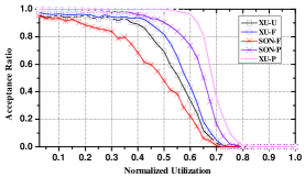
(a) Under different $U_{norm}$.

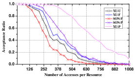
(b) Under different $\sum_{\tau_{i}\in\tau}N_{i,q}$.

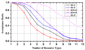
(c) Under different $|\Theta|$.

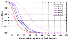
(d) Under different $\max_{\forall\tau_{i}}\{L_{i,q}\}$.

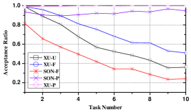
(e) Under different $n$.

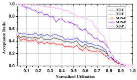
(f) Under realisitic OpenMP programs.

Figure 5: Comparisons with the state-of-the-art.

We first compare the three approaches with randomly generated task systems. The DAG tasks are generated as follows:

• Task Graph $G_{i}=\langle V_{i},E_{i}\rangle$: The task graph of each task is generated using the Erdös-Rényi method $G(|V_{i}|,p)$ [15]. For each task, the number of vertices $|V_{i}|$ is randomly chosen in $[100,400]$. The WCET of each vertex is randomly picked in $[250,600]$. The metrics of the number and WCETs of vertices are consistent with the measurement results in [16]. For each possible edge we generate a random value in $[0,1]$ and add the edge to the graph only if the generated value is less than a predefined threshold $p=0.1$. The same as in [17], a minimum number of additional edges are added to make a task graph weakly connected.

• Deadline and Period: The deadline $D_{i}$ of each task $\tau_{i}$ is generated in a similar way with [9]: after $\mathcal{L}_{i}$ is fixed, $D_{i}$ is generated according to a ratio between $\mathcal{L}_{i}$ and $D_{i}$ randomly chosen in $\{0.125,0.25\}$. The period $T_{i}$ is set to be equal to $D_{i}$.

• Resource: The number of resource types is in the range $[1,12]$. The number of accesses to each resource by all tasks $\sum_{\tau_{i}\in\tau}N_{i,q}$ is in the range $[16,1008]$, and is randomly distributed to different tasks. The maximal locking time $\max_{\forall\tau_{i}}\{L_{i,q}\}$ of each resource is in the range $[5,60]$ and each $L_{i,q}$ is randomly picked in $[1,\max_{\forall\tau_{i}}\{L_{i,q}\}]$.

Since we only focus on heavy tasks, a task with $U_{i}<1$ is discarded until a heavy task is generated during the generation of each task. For each task set, we generate $n$ tasks where $n$ is in $[1,14]$. The normalized utilization $U_{norm}$ (the ratio between the total utilization and the number of processors) of each task set is predefined, which will be explained in detail for the configuration of each figure. After we generate all tasks in a task set, we can compute the total utilization $U_{\sum}$, then we set the number of processors according to the formula $m=\lceil\frac{U_{\sum}}{U_{norm}}\rceil$. The number of processors could become quite large (far more than 10 processors) when $U_{\sum}$ is relatively low (e.g., lower than 0.2) or the number of tasks in a task set is large (e.g., more than 6 tasks). For each configuration (corresponding to one point on the X-axis), we generate $1000$ task sets.

In Figure 5.(a)-(e), we set a basic configuration and in each group of experiments vary one parameter while keeping others unchanged. The basic configuration is as follows: $n=4$, $U_{norm}=0.5$, the number of resource types is 4, $\sum_{\tau_{i}\in\tau}N_{i,q}=256$ and $\max_{\forall\tau_{i}}\{L_{i,q}\}=15$.

Figure 5.(a) shows acceptance ratios of all tests under different normalized utilizations (X-axis). Figure 5.(b) evaluates the acceptance ratios under different $\sum_{\tau_{i}\in\tau}N_{i,q}$. We can observe that the acceptance ratios of all tests decrease as $\sum_{\tau_{i}\in\tau}N_{i,q}$ increases. Figure 5.(c) shows the acceptance ratios under different number of resource types. The acceptance ratios of all tests decrease as the number of resource types increases. In Figure 5.(d), resources are generated with different $\max_{\forall\tau_{i}}\{L_{i,q}\}$. The schedulability of all tests decreases as $\max_{\forall\tau_{i}}\{L_{i,q}\}$ increases. In Figure 5.(e), we generate different number of tasks in each configuration. The schedulability of XU-U, XU-F and SON-F decreases as the number of tasks increases whereas the schedulability of tests for priority order, i.e., XU-P and SON-P, is hardly affected by the number of tasks.

From the above results we see that tests for priority-order perform better than those for FIFO-order and unordered, and our approaches consistently outperform the state-of-the-art under different parameter settings: XU-P outperforms SON-P and XU-F outperforms SON-F. In particular, even if XU-U adopts less queue order information, it still consistently outperforms SON-F due to our new analysis techniques which systematically analyze the blocking time that may delay the finishing time of a parallel task and jointly consider the impact of blocking time to both the total workload and the longest path length.

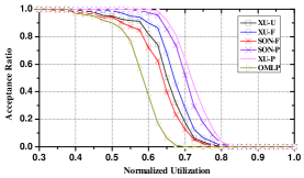
(a) Under different $U_{norm}$.

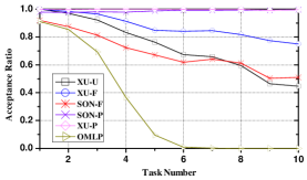
(b) Under different $n$.

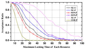
(c) Under different $\max_{\forall\tau_{i}}\{L_{i,q}\}$.

Figure 6: Comparisons with OMLP.

In the following, we conduct experiments to evaluate the performance of both [9] and our results in comparison with locking protocols for sequential tasks. That is, we try to find a straightforward way to extend locking protocols for sequential tasks to paralleled tasks, such that the points we make in Section 3 can be more clear. Some modern analysis techniques for sequential tasks use Linear Programming (LP) to achieve more precise performance, e.g., [18, 14], which are not included due to the following reasons. First, the blocking times are defined under schedulability tests for sequential tasks which can not be directly applied for parallel tasks (some significant modifications and techniques are required and it is not trivial). Second, the LP-based techniques run with significant computing resources and time since they are with quite high complexity (weeks on clustered computers as provided by the authors of [9]) whereas our tests and [9] are polynomial. OMLP is a well-known locking protocol of clustered scheduling for sequential tasks [13] which is also the most relevant work with this paper (DAG tasks scheduled under federated scheduling can be regarded as sequential tasks scheduled on clusters). In Fig.6, we apply OMLP on DAG tasks in a straightforward manner where each vertex in a DAG task is regarded as an independent sequential task. We first randomly distribute the generated requests of each task to its vertices. The priorities of all vertices in a DAG task are set the same as their indexes, and a vertex with a smaller index has a higher priority. We first compute the S-oblivious PI-blocking for each vertex according to the blocking analysis techniques presented in [13] and then add the PI-blocking to the WCET of the vertex, after which the longest length among all paths and the WCET of all vertices of $\tau_{i}$ are denoted by $\mathcal{L}_{i}^{{}^{\prime}}$ and $\mathcal{C}_{i}^{{}^{\prime}}$ respectively. Then we use the general schedulability test of federated scheduling for each DAG task [6], i.e., the response time of task $\tau_{i}$ is computed by $R_{i}\leq\mathcal{L}_{i}^{{}^{\prime}}+\frac{\mathcal{C}_{i}^{{}^{\prime}}-\mathcal{L}_{i}^{{}^{\prime}}}{m_{i}}$. The schedualbility of the task set is decided in a similar way with Algorithm 3 (the only difference is on the computation of $R_{i}$).

In Figure 6.(a)-(c), we set a basic configuration and in each group of experiments vary one parameter while keeping others unchanged. The basic configuration is as follows: $n=4$, $U_{norm}=0.6$, the number of resource types is 9, $\sum_{\tau_{i}\in\tau}N_{i,q}=60$ and $\max_{\forall\tau_{i}}\{L_{i,q}\}=15$. In comparison with the basic configuration of Figure 5, we have significantly reduced the total number of resource accesses to evaluate the performance of our results in a system with a modicum number of accesses (the case that is more close to the practical scenarios). It may be noticed that both our work and [9] are based on the classic Graham’s bound [19]. Thus if there are no resource access contentions, the schedulabilities of our result and [9] are the same, and of course the gap of the performance between our results and [9] becomes more significant when there are more resource access contentions. From Figure 6, we can observe that our results still outperform [9]. Moreover, even more concrete information are used (i.e., the exact distributions of requests), directly applying locking protocols and associated blocking analysis techniques for sequential tasks on DAG tasks is quite pessimistic (as discussed in Section 3).

6.2 Realistic OpenMP Programs

In the following, we evaluate the three approaches with workload generated according to realistic OpenMP programs. OpenMP supports task parallelization since version 3.0 [20], which can be modeled as DAG models [16]. We collect $8$ OpenMP programs (see Table. II) using C language from different benchmark suits and transform them into DAG model. We measure the $\mathcal{C}_{i}$ and $\mathcal{L}_{i}$ of each program and $N_{i,q}$ and $L_{i,q}$ to each shared resource by each task on a hardware platform with Intel i7-7820HQ CPU@2.90GHz, cache size of 8MB and total memory of 4GB. The run time compiling environment is Ubuntu 12.04.5 LTS with gcc 4.9.4. We consider $10$ different types of resources, where the first $4$ are shared data objects in the operating kernel accessed via system calls (i.e., time) or library calls (i.e., fprintf, printf, malloc). The remaining $6$ are shared data structures or non-reusable routines protected by # pragma omp critical in the OpenMP program.

The measurement results are summarized in Table II, where the time unit is $\mu s$. Note that the measurement results are not guaranteed to be safe upper bounds of the desired parameters. In order to obtain their safe upper bounds, a comprehensive static analysis covering all the hardware and software behaviors is required. In this paper, we simply use these results to approximately represent the workload characteristics of these OpenMP programs. It may be notices that the number of types of shared resources that each program may access is not large. The resources accessing behaviors of programs in bots-1.1.2 are similar because of that they are all commutative algorithms and may use some similar library calls such as "malloc". These features does not affect our evaluations, and the main purpose of our evaluations is to show the impact to the schedulability of realistic parallel programs with shared resources and the schedulabilities under different methods.

TABLE II: Measurement results of OpenMP programs.

Benchmark	Application	$\mathcal{C}_{i}$	$\mathcal{L}_{i}$	$\ell_{0}$		$\ell_{1}$		$\ell_{2}$		$\ell_{3}$		$\ell_{4}$		$\ell_{5}$		$\ell_{6}$		$\ell_{7}$		$\ell_{8}$		$\ell_{9}$
				$N$	$L$	$N$	$L$	$N$	$L$	$N$	$L$	$N$	$L$	$N$	$L$	$N$	$L$	$N$	$L$	$N$	$L$	$N$	$L$
bots-1.1.2 [21]	alignment.for	313168	11446	22	2	1	2	2	2	0	0	0	0	0	0	0	0	0	0	0	0	0	0
	alignment.single	315981	9980	22	2	1	2	2	2	0	0	0	0	0	0	0	0	0	0	0	0	0	0
	fft	274	58	21	2	1	4	2	2	0	0	0	0	0	0	0	0	0	0	0	0	0	0
	fib	353	20	20	2	0	0	2	2	0	0	0	0	0	0	0	0	0	0	0	0	0	0
	sort	1757	217	20	2	2	4	2	2	0	0	0	0	0	0	0	0	0	0	0	0	0	0
	floorplan	5843	92	36	2	6	1	2	2	0	0	4	1	0	0	0	0	0	0	0	0	0	0
OpenMPMicro [22]	MatrixMultiplication	5873246	106983	0	0	3	7	0	0	5	4	0	0	0	0	0	0	0	0	0	0	0	0
	Square	50000812	1000066	0	0	0	0	0	0	0	0	0	0	20	5	50	1	50	105	50	79	50	1

For each task set, we pick $n$ programs (each being a DAG task) in Table II, where $n$ is randomly chosen in $[2,5]$. The deadline $D_{i}$ of each task and the number of processors in the system are set in the same way as Section 6.1.

Fig. 5.(f) shows acceptance ratios of all tests under different normalized utilizations (X-axis). We can observe that the acceptance ratios of all tests decrease in comparison with Fig. 5.(a). This is because some applications have relatively short deadlines and periods by our task generation method, and thus have low tolerance to blocking time caused by other tasks. Nevertheless, the results have the same trend as in Fig. 5.(a): XU-F consistently outperforms SON-F while XU-P outperforms SON-P.

7 Related Work

There is plentiful of literature on scheduling algorithms and analysis techniques for the parallel real time tasks [6, 7, 8, 23, 24], which all assume tasks to be independent from each other and do not consider the locking issue.

Real-time locking protocols are well supported in uniprocessor systems. The Priority Inheritance Protocol (PIP) [3] is the first solution to address the priority inversion problem. There are several optimal protocols for uniprocessor real-time task systems, such as Multiprocessor Stack Resource Policy (SRP) [2] and Priority Ceiling Protocol (PCP) [3] which guarantee bounded blocking time for a single resource access request and ensure deadlock freedom.

On multiprocessors, there are two major lock types: spin locks and suspension-based semaphores. Much work has been done for partitioned multiprocessor scheduling, such as MPCP [5] and DPCP [25] and the Multiprocessor Stack Resource Policy (MSRP) [26]. The Flexible Multiprocessor Locking Protocol (FMLP) [10] is a family of locking protocols which support both global and partitioned scheduling. The Parallel Priority Ceiling Protocol (P-PCP) [27] is an extension of the PIP that attempts to avoid certain unfavorable blocking situations. The family of $O(m)$ Locking Protocols (OMLP) [4, 13] is a suite of suspension-based locking protocols that have proved to be asymptotically optimal under suspension-oblivious analysis. Lakshmanan et al. [28] proposed the Multiprocessor Priority Ceiling Protocol with virtual spinning and Faggioli et al. [29] proposed a locking protocol for reservation-based schedulers that includes preemptable spinning.

A recent work considering locks for parallel real-time task model is [9], which adopts the federated scheduling framework with spin locks. As mentioned before, [9] analyzes the impact of the blocking time to the total workload and the longest path length separately, which leads to significant pessimism in analysis precision. The contribution of this paper is to address this pessimism in [9].

The locking protocols have been studied with other graph-based task models, such as the DRT model [30] and multi-frame task model[31]. However, these models are still sequential (multiple edges going out from a vertex have conditional branching semantics rather than forking).

8 CONCLUSIONS

We study the analysis of parallel real-time tasks with spin locks in three different orders under federated scheduling. A recent work [9] developed analysis techniques for this problem, which are pessimistic since all blocking time are assumed to delay the finishing time of a parallel task and the blocking time to the total workload and the longest path length of each task is analyzed separately. In this paper, we develop new schedulability and blocking analysis techniques to improve the analysis precision. In our future work, we will investigate blocking analysis on other (finer-grained) models.

Xu Jiang has received his BS degree in computer science from Northwestern Polytechnical University, China in 2009, received the MS degree in computer architecture from Graduate School of the Second Research Institute of China Aerospace Science and Industry Corporation, China in 2012, and PhD from Beihang University, China in 2018. Currently, he is working in Northeastern University, China. His research interests include real-time systems, parallel and distributed systems and embedded systems.

Nan Guan is currently an assistant professor at the Department of Computing, The Hong Kong Polytechnic University. Dr Guan received his BE and MS from Northeastern University, China in 2003 and 2006 respectively, and a PhD from Uppsala University, Sweden in 2013. Before joining PolyU in 2015, he worked as a faculty member in Northeastern University, China. His research interests include real-time embedded systems and cyber-physical systems. He received the EDAA Outstanding Dissertation Award in 2014, the Best Paper Award of IEEE Real-time Systems Symposium (RTSS) in 2009, the Best Paper Award of Conference on Design Automation and Test in Europe (DATE) in 2013.

He Du is currently a Ph.D. candidate at School of Computer Science and Engineering, Northeastern University. She received the Bachelor degree from Northeastern University, Shenyang, China, in 2015. Her research interests focus on parallelism program analyze and multiprocessor real-time scheduling.

Weichen Liu received the B.Eng. and M.Eng. degrees from the Harbin Institute of Technology, Harbin, China, and the Ph.D. degree from the Hong Kong University of Science and Technology, Hong Kong. He is an Assistant Professor with the School of Computer Science and Engineering, Nanyang Technological University, Singapore. He has authored and co-authored over 70 publications in peer-reviewed journals, conferences, and books. His current research interests include embedded and real-time systems, multiprocessor systems, and network-on-chip. Dr. Liu was a recipient of the Best Paper Candidate Awards from ASP-DAC 2016, CASES 2015, and CODES+ISSS 2009, the Best Poster Awards from RTCSA 2017 and AMD-TFE 2010, and the most popular Poster Award from ASP-DAC 2017.

Wang Yi received the PhD in computer science from Chalmers University of Technology, Sweden, in 1991. He is a chair professor with Uppsala University. His interests include models, algorithms and software tools for building and analyzing computer systems in a systematic manner to ensure predictable behaviors. He was awarded with the CAV 2013 Award for contributions to model checking of real-time systems, in particular the development of UPPAAL, the foremost tool suite for automated analysis and verification of real-time systems. For contributions to real-time systems, he received Best Paper Awards of RTSS 2015, ECRTS 2015, DATE 2013 and RTSS 2009, Outstanding Paper Award of ECRTS 2012 and Best Tool Paper Award of ETAPS 2002. He is on the steering committee of ESWEEK, the annual joint event for major conferences in embedded systems areas. He is also on the steering committees of ACM EMSOFT (co-chair), ACM LCTES, and FORMATS. He serves frequently on Technical Program Committees for a large number of conferences, and was the TPC chair of TACAS 2001, FORMATS 2005, EMSOFT 2006, HSCC 2011, LCTES 2012 and track/topic Chair for RTSS 2008 and DATE 2012-2014. He is a member of Academy of Europe (Section of Informatics) and a fellow of the IEEE.

References

- [1] M. Jones, “What really happened on mars rover pathfinder,” The Risks Digest, vol. 19, no. 49, pp. 1–2, 1997.
- [2] T. P. Baker, “Stack-based scheduling of realtime processes,” Real-Time Systems, vol. 3, no. 1, pp. 67–99, 1991.
- [3] L. Sha, R. Rajkumar, and J. P. Lehoczky, “Priority inheritance protocols: An approach to real-time synchronization,” IEEE Transactions on computers, vol. 39, no. 9, pp. 1175–1185, 1990.
- [4] B. B. Brandenburg and J. H. Anderson, “Optimality results for multiprocessor real-time locking,” in RTSS. IEEE, 2010, pp. 49–60.
- [5] R. Rajkumar, “Real-time synchronization protocols for shared memory multiprocessors,” in ICDCS. IEEE, 1990, pp. 116–123.
- [6] J. Li, J. J. Chen, and et.al, “Analysis of federated and global scheduling for parallel real-time tasks,” in ECRTS, 2014.
- [7] C. Maia, M. Bertogna, and et.al, “Response-time analysis of synchronous parallel tasks in multiprocessor systems,” in RTNS, 2014.
- [8] X. Jiang, X. Long, and et.al, “On the decomposition-based global edf scheduling of parallel real-time tasks,” in RTSS, 2016.
- [9] S. Dinh, J. Li, K. Agrawal, C. Gill, and C. Lu, “Blocking analysis for spin locks in real-time parallel tasks,” IEEE Transactions on Parallel and Distributed Systems, vol. 29, no. 4, pp. 789–802, 2018.
- [10] A. Block, H. Leontyev, B. B. Brandenburg, and J. H. Anderson, “A flexible real-time locking protocol for multiprocessors,” in RTCSA. IEEE, 2007, pp. 47–56.
- [11] A. Wieder and B. B. Brandenburg, “On spin locks in autosar: Blocking analysis of fifo, unordered, and priority-ordered spin locks,” in RTSS. IEEE, 2013, pp. 45–56.
- [12] B. Brandenburg and J. H. Anderson, “Scheduling and locking in multiprocessor real-time operating systems,” Ph.D. dissertation, Citeseer, 2011.
- [13] B. B. Brandenburg and J. H. Anderson, “The omlp family of optimal multiprocessor real-time locking protocols,” Design automation for embedded systems, vol. 17, no. 2, pp. 277–342, 2013.
- [14] M. Yang, A. Wieder, and B. B. Brandenburg, “Global real-time semaphore protocols: A survey, unified analysis, and comparison,” in RTSS. IEEE, 2015, pp. 1–12.
- [15] D. Cordeiro, G. Mounié, and et.al, “Random graph generation for scheduling simulations,” in ICST, 2010.
- [16] Y. Wang, N. Guan, J. Sun, M. Lv, Q. He, T. He, and W. Yi, “Benchmarking openmp programs for real-time scheduling,” in RTCSA. IEEE, 2017, pp. 1–10.
- [17] A. Saifullah, D. Ferry, and et.al, “Parallel real-time scheduling of dags,” Parallel and Distributed Systems, IEEE Transactions on, 2014.
- [18] A. Wieder and B. B. Brandenburg, “On spin locks in autosar: Blocking analysis of fifo, unordered, and priority-ordered spin locks,” RTSS, 2013.
- [19] R. L. Graham, “Bounds on multiprocessing timing anomalies,” SIAM journal on Applied Mathematics, 1969.
- [20] O. Board, “Openmp application program interface version 3.0,” in The OpenMP Forum, Tech. Rep, 2008.
- [21] A. Duran, X. Teruel, R. Ferrer, X. Martorell, and E. Ayguade, “Barcelona openmp tasks suite: A set of benchmarks targeting the exploitation of task parallelism in openmp,” in ICPP. IEEE, 2009, pp. 124–131.
- [22] V. V. Dimakopoulos, P. E. Hadjidoukas, and G. C. Philos, “A microbenchmark study of openmp overheads under nested parallelism,” in International Workshop on OpenMP. Springer, 2008, pp. 1–12.
- [23] J. Fonseca, G. Nelissen, and V. Nélis, “Improved response time analysis of sporadic dag tasks for global fp scheduling,” in Proceedings of the 25th international conference on real-time networks and systems. ACM, 2017, pp. 28–37.
- [24] X. Jiang, N. Guan, X. Long, and W. Yi, “Semi-federated scheduling of parallel real-time tasks on multiprocessors,” in RTSS. IEEE, 2017, pp. 80–91.
- [25] R. Rajkumar, L. Sha, and J. P. Lehoczky, “Real-time synchronization protocols for multiprocessors,” in RTSS. IEEE, 1988, pp. 259–269.
- [26] P. Gai, G. Lipari, and M. Di Natale, “Minimizing memory utilization of real-time task sets in single and multi-processor systems-on-a-chip,” in RTSS. IEEE, 2001, pp. 73–83.
- [27] A. Easwaran and B. Andersson, “Resource sharing in global fixed-priority preemptive multiprocessor scheduling,” in RTSS. IEEE, 2009, pp. 377–386.
- [28] K. Lakshmanan, D. de Niz, and R. Rajkumar, “Coordinated task scheduling, allocation and synchronization on multiprocessors,” in RTSS. IEEE, 2009, pp. 469–478.
- [29] D. Faggioli, G. Lipari, and T. Cucinotta, “The multiprocessor bandwidth inheritance protocol,” in ECRTS. IEEE, 2010, pp. 90–99.
- [30] N. Guan, P. Ekberg, M. Stigge, and W. Yi, “Resource sharing protocols for real-time task graph systems,” in ECRTS. IEEE, 2011, pp. 272–281.
- [31] P. Ekberg, N. Guan, M. Stigge, and W. Yi, “An optimal resource sharing protocol for generalized multiframe tasks,” Journal of Logical and Algebraic Methods in Programming, vol. 84, no. 1, pp. 92–105, 2015.