Accretion Properties of PDS 70b with MUSE

Abstract

We report a new evaluation of the accretion properties of PDS 70b obtained with VLT/MUSE. The main difference from previous studies in Haffert et al. (2019) and Aoyama & Ikoma (2019) is in the mass accretion rate. Simultaneous multiple line observations, such as H$\alpha$ and H$\beta$, can better constrain the physical properties of an accreting planet. While we clearly detected H$\alpha$ emissions from PDS 70b, no H$\beta$ emissions were detected. We estimate the line flux of H$\beta$ with a 3-$\sigma$ upper limit to be 2.3 $\times$ 10^-16 erg s^-1 cm^-2. The flux ratio $F_{\rm H\beta}$/$F_{\rm H\alpha}$ for PDS 70b is $<$ 0.28. Numerical investigations by Aoyama et al. (2018) suggest that $F_{\rm H\beta}$/$F_{\rm H\alpha}$ should be close to unity if the extinction is negligible. We attribute the reduction of the flux ratio to the extinction, and estimate the extinction of H$\alpha$ ($A_{\rm H\alpha}$) for PDS 70b to be $>$ 2.0 mag using the interstellar extinction value. By combining with the H$\alpha$ linewidth and the dereddening line luminosity of H$\alpha$, we derive the PDS 70b mass accretion rate to be $\gtrsim$ 5 $\times$ 10^-7 $M_{\rm Jup}$ yr^-1. The PDS 70b mass accretion rate is an order of magnitude larger than that of PDS 70. We found that the filling factor $f_{\rm f}$ (the fractional area of the planetary surface emitting H$\alpha$) is $\gtrsim$0.01, which is similar to the typical stellar value. The small value of $f_{\rm f}$ indicates that the H$\alpha$ emitting areas are localized at the surface of PDS 70b.



1 Introduction

Gas giant planets growing in a protoplanetary disk gain their mass via mass accretion from the parent disk until their host star loses its gas disk (e.g., Hayashi et al., 1985). A part of the gas flow from the outer disk accretes onto gas giant planets while the rest of the flow passes over the planets toward the central star. The relationship between the host star and planets in the mass accretion rate depends on the planetary mass and the disk’s properties (e.g., Lubow et al., 1999; Tanigawa & Tanaka, 2016). Numerical simulations of disk–planet interactions show that the mass accretion rate of a 1-$M_{\rm Jup}$ planet can reach up to $\sim$90 % of the rate of mass accretion from the outer disk, i.e., the planetary mass accretion rate is an order of magnitude larger than the stellar rate (Lubow & D’Angelo, 2006). As predicted by planet population synthesis models (e.g., Ida & Lin, 2004), when the gas accretion onto planets is sufficiently large, gas giant planets can form more than sub-Jovian planets. On the other hand, microlensing observations show that the number of sub-Jovian planets is dominant in the planetary mass function (Suzuki et al., 2018). The mass accretion onto a planet determines the final mass of the planet (e.g., Tanigawa & Ikoma, 2007) and thus investigating the planetary mass accretion process informs our understanding of planet formation.

Direct imaging allows the study of gas accretion in young planets via H_I recombination lines such as H$\alpha$ at 656.28 nm (e.g., Zhou et al., 2014; Sallum et al., 2015; Santamaría-Miranda et al., 2018; Wagner et al., 2018; Haffert et al., 2019). Although the gas temperature in the surface layers of protoplanetary disks is expected to be high enough ($T\sim$ 10⁴ K) to emit H_I recombination lines (e.g., Kamp & Dullemond, 2004), their emissions may be too weak to be detected due to the low density of the disk surface. Therefore, the observed H$\alpha$ emissions from point-like sources reported in the literature have been attributed to the abundant cold gas around planets in the disk midplane being heated by gas accretion onto planets. In case of T Tauri stars, two important heating mechanisms in the standard accretion processes have been investigated to understand stellar accretion processes (Bertout et al., 1988; Koenigl, 1991; Popham et al., 1993; Calvet & Gullbring, 1998). The first is viscous heating in the boundary layer where the faster rotating Keplerian disk connects with the slowly rotating star. The other is accretion shock heating by magnetospheric accretion, in which the gas flow from the midplane of a circumstellar disk shocks the central star by a strong stellar magnetic field. Theoretical studies on planetary accretion processes have also investigated accretion shock heating at the surface of planets (e.g., Zhu, 2015; Tanigawa et al., 2012; Aoyama et al., 2018).

Recently, Aoyama & Ikoma (2019) demonstrated that the H$\alpha$ spectral line-width and luminosity can be used to constrain the planetary mass and the rate of mass accretion onto protoplanets, by applying radiation-hydrodynamic models of the shock-heated accretion flow (Aoyama et al., 2018). A good example of robustly detected accreting planets at tens of au from a central star is the PDS 70 planetary system. This system includes a weakly accreting young star (spectral type of K7, mass of 0.8 $M_{\odot}$, accretion rate of 6 $\times$ 10^-11 $M_{\odot}$  yr^-1, age of 5 Myr, distance of 113 pc; Pecaut & Mamajek, 2016; Keppler et al., 2019; Haffert et al., 2019; Müller et al., 2018; Gaia Collaboration et al., 2018) associated with two planetary-mass companions (Haffert et al., 2019; Isella et al., 2019; Christiaens et al., 2019a, b; Keppler et al., 2018; Müller et al., 2018; Wagner et al., 2018). Aoyama & Ikoma (2019) estimated that PDS 70b’s mass and mass accretion rate are $\sim$12 $M_{\rm Jup}$ and $\sim$4 $\times$ 10^-8 $M_{\rm Jup}$ yr^-1, respectively, while the values for PDS 70c are $\sim$10 $M_{\rm Jup}$ and $\sim$1 $\times$ 10^-8 $M_{\rm Jup}$ yr^-1. To convert the H$\alpha$ luminosity into the mass accretion rate, we need to constrain the fractional area of the planetary surface emitting H$\alpha$, which is often termed the filling factor $f_{\rm f}$, and the degree of extinction $A_{\rm H\alpha}$ of H$\alpha$. However, these values have been poorly measured in observations.

In this paper, we revisit the accretion properties of PDS 70b by re-analyzing archive data used in Haffert et al. (2019). We aim to estimate the physical quantities related to planetary mass accretion with the help of the theoretical study by Aoyama & Ikoma (2019). We will demonstrate that by combining a 3-$\sigma$ upper limit in the flux ratio of $F_{\rm H\beta}$/$F_{\rm H\alpha}$, the H$\alpha$ line luminosity, and the H$\alpha$ linewidth, we can constrain the filling factor $f_{\rm f}$, the $\rm H\alpha$ extinction $A_{\rm H\alpha}$, and the mass accretion rate onto the planet.

2 Archival Data and Stellar Spectral Subtraction

2.1 Archival Data

Observations of PDS 70 were made with the optical integral field spectrograph MUSE (Multi Unit Spectroscopic Explorer; Bacon et al., 2010) at the VLT (Very Large Telescope) on June 20th 2018 (UT) under the clear sky conditions with optical seeing of 0.^′′70–0.^′′81, as part of the commissioning runs of the Narrow-Field Mode (NFM). The adaptive optics (AO) system for MUSE consists of the four laser guide star (LGS) facility and the deformable secondary mirror (DSM). The LGS wavefront sensors measure the turbulance in atmosphere, and the DSM corrects a wave-front to provide near diffraction limited images. The data used in this work (a field of view: 7.^′′42 $\times$ 7.^′′43, a spatial sampling: 25 $\times$ 25 mas², a spectral range: 4650 to 9300 Å, a resolving power: 2484 $\pm$ 5 at 6500.0 Å) are publicly available on the ESO archive. Six individual raw frames with an exposure time of 300 seconds were obtained and calibrated with the MUSE pipeline v2.6 (Weilbacher et al., 2012; see Haffert et al., 2019 for more details about data). The absolute flux was also calibrated in the pipeline where the flux calibration curve is derived from both an atmospheric extinction curve at Cerro Paranal and a spectro-photometric standard star stored as MUSE master calibrations. The apparent magnitude of PDS 70 in calibrated MUSE data at 6905 to 8440 Å correspoding to the Sloan $i^{\prime}$ band filter is measured to 12.0 $\pm$ 0.1 mag, which is fainter than the literature value of $i^{\prime}=$11.1 $\pm$ 0.1 mag (Henden et al., 2015). In the following post-processing, we used an image size of 40 $\times$ 40 spatial pixels (corresponding to 1^′′ $\times$ 1^′′) around the central star with a high signal-to-noise (SN) ratio. In changing the size, we found that this size maximized the SN of PDS 70b. Furthermore, since there are no signals in $\sim$5780 to $\sim$6050 Å to avoid contamination by sodium light from LGS, we removed them from the data.

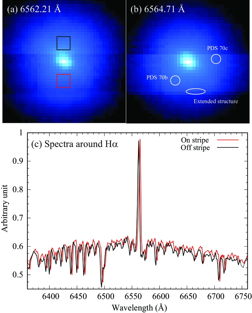
Figure 4: Stripe patterns in the vicinity of the central star at 6562.21 Å in panel (a) and 6564.71 Å in panel (b). The image size is 1^′′ $\times$ 1^′′. The white circles and ellipse indicate the positions of PDS 70b, PDS 70c, and a possible extended structure. (c) Spectra in the stripe (red) and in the off-stripe (black) at the red and black square regions in panel (a), respectively. The stripe pattern is induced by a wavelength shift possibly due to calibration errors.

After the basic calibration with the MUSE pipeline via a scientific workflow of EsoReflex (Freudling et al., 2013), we extracted six data cubes and inspected them carefully. We found that five of the data cubes have a relatively strong stripe pattern in the vicinity of the central star (Figure 4 in Appendix), induced by a wavelength shift due to possible calibration errors. Since we see no wavelength shift in one data cube, we conducted cross-correlation analyses to correct the wavelength shift. The FWHM of PSF in the final image was 66 mas at 6562.8 Å.

2.2 Stellar Spectral Subtraction

To subtract the stellar spectra of PDS 70 at each spatial pixel, we followed the methods used in Haffert et al. (2019). An essential point is to construct reference spectra from the most correlated components obtained from principal component analysis (PCA; see the basis of PCA given by Jee et al., 2007). Before applying PCA, we normalized each spectrum by the median values of each spectrum (a purple line in Figure 6 in Appendix). We then calibrated a fake continuum pattern, as shown in Figure 5 in the Appendix, where we show that the stellar spectra are different from the halo spectra at 300 mas from the stellar position. This is because the degree of central concentration of the stellar flux is higher at longer wavelengths due to the better AO performance at longer wavelengths. To calibrate this fake continuum, we generated median spectra for 40 $\times$ 40 spatial pixels in six data cubes (a blue line in Figure 6). We chose the median to avoid residual bad/hot pixels. After dividing each spectrum by the median spectrum (a red line in Figure 6), we smoothed each divided spectrum by a Gaussian function with a kernel of 230 spectral channels (a black line in Figure 6). Finally, we divided each normalized spectrum (the purple line in Figure 6) by the smoothed spectrum (the black line in Figure 6) to correct the fake continuum (a yellow line in Figure 6).

We applied PCA to 9,600 spectra (six frames with 40 $\times$ 40 spatial pixels) and found the optimum number of components to subtract to be 1, by maximizing the SN of PDS 70b. After subtracting reference spectra for each spatial pixel, we recovered the unit (10^-20 erg s^-1 cm^-2 Å^-1) in the image by performing inverse processes of above normalization. Two data cubes out of six were removed from the final image since they degraded the data quality, i.e., gave a worse SN of PDS 70b. The total exposure time after removing the two cubes was 1,200 s. The final images are shown in Figure 1, in which the H$\alpha$ and H$\beta$ images are constructed with three (656.096, 656.221, and 656.346 nm) and one (486.096 nm) wavelength channels, respectively. Astrometry of the two planets is summarized in Table 1.

2.3 Flux Measurement

The H$\alpha$ fluxes were measured with a box aperture of 3 $\times$ 3 pixels centered on PDS 70b and c in the combined image of three channels. The errors of H$\alpha$ and H$\beta$ per spectral channel were estimated from the standard deviation of the flux within the box aperture (3 $\times$ 3 pixels) at the planetary positions in a continuum spectra, i.e., $\sim$6570 to $\sim$6700 Å and $\sim$4800 to $\sim$4930 Å for H$\alpha$ and H$\beta$, respectively. The SN ratios of H$\alpha$ were 27 and 10 for PDS 70b and c, respectively (Table 1), while the peak SN ratios along the spectral direction were 20 and 9 for PDS 70b and c, respectively (Figure 1).

To recover the missing flux, we applied two flux calibrations. The first was an aperture correction (Howell, 1990) in which we recovered the missing flux due to the small aperture. The other was a flux correction in which we estimated the lost flux during the PSF subtraction. In the aperture correction, the correction factors (between the box aperture of 3 $\times$ 3 pixels and a circular aperture of 70 pixels in radius) derived by photometry of the primary star were 6.65 and 16.9 for H$\alpha$ and H$\beta$, respectively. Since the AO performance is better at longer wavelengths, the correction factor of H$\alpha$ is smaller than that of H$\beta$. We then inspected the extent to which the point source flux decreased during the PSF subtraction. Positive fake sources were injected in the H$\alpha$ and H$\beta$ channels, and the PSF subtraction process was re-run. The fake sources were injected at the separations of PDS 70b and c, and at position angles of 0$\arcdeg$ to 345$\arcdeg$ with 15$\arcdeg$ steps, except the planetary positions, and with fluxes corresponding to those of PDS 70b and c without flux calibrations. Regarding the H$\beta$ flux, we used a 3-$\sigma$ value as the input flux. The results show that the flux decreased to 90%, 98%, 90%, and 95% for PDS 70b at H$\alpha$, PDS 70c at H$\alpha$, PDS 70b at H$\beta$, and PDS 70c at H$\beta$, respectively. The corrected line fluxes and their errors are shown in Table 1. The linewidths were measured by fitting a Gaussian profile to the H$\alpha$ spectra with the fit function in GNUPLOT.

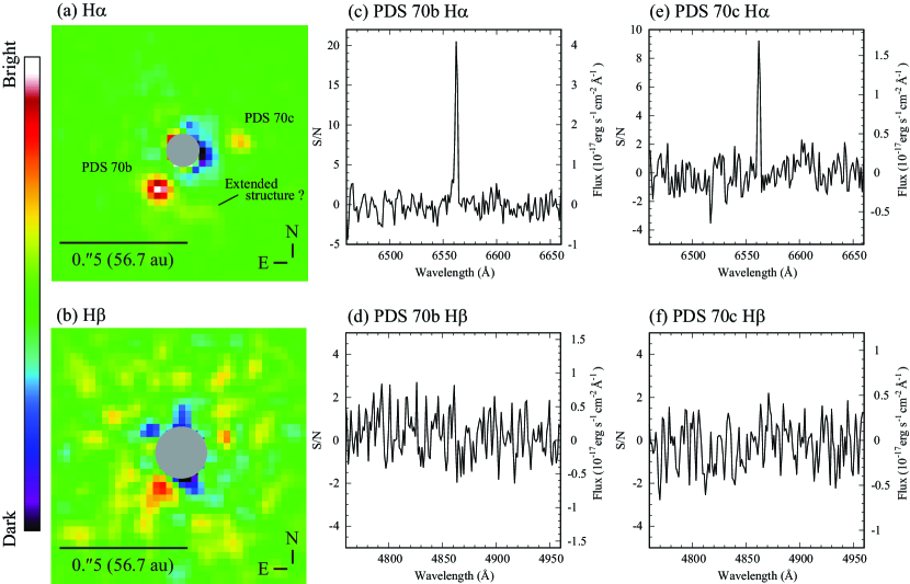
Figure 1: H$\alpha$ and H$\beta$ images of PDS 70b and c and their spectra. (a and b) H$\alpha$ and H$\beta$ images generated from three (3.75-Å width) and one (1.25 Å width) spectral channels centered at 6562.21 and 4860.96 Å, respectively, and are convolved with a Gaussian kernel of 2 pixels in radius. The central regions in panels (a) and (b) are masked with gray circles of 125 and 200 mas diameter, respectively. (c to f) Spectra of PDS 70b and c at H$\alpha$ and H$\beta$ in a box aperture of 3 $\times$ 3 pixels. Neither flux calibration (i.e., aperture and flux correction described in § 2.3) nor dereddening correction derived in § 4.2 is applied to the spectra.

Table 1: Line flux with flux calibration, line profile, and astrometry of PDS 70b and c

Name	Line flux	Line center	10% linewidth	50% linewidth	P.A.	Separation
	(10-16 erg s-1 cm-2)	(km s-1)	(km s-1)	(km s-1)	($\arcdeg$)	(mas; au)
PDS 70b (H$\alpha$)	8.1 $\pm$ 0.3	$-$18 $\pm$ 4	213 $\pm$ 15	114 $\pm$ 8	147 $\pm$ 8	178 $\pm$ 25; 20.2 $\pm$ 2.8
(H$\beta$)	$<$2.3	—	—	—	—
PDS 70c (H$\alpha$)	3.1 $\pm$ 0.3	$-$26 $\pm$ 6	200 $\pm$ 24	107 $\pm$ 13	278 $\pm$ 6	225 $\pm$ 25; 25.5 $\pm$ 2.8
(H$\beta$)	$<$1.6	—	—	—	—

3 Results

Figure 1 and Table 1 show our re-analysis results. They are largely similar with those in Haffert et al. (2019). As already reported in Haffert et al. (2019), we also clearly detected H$\alpha$ emissions from PDS 70b and c, while H$\beta$ emissions were not detected. The peak SN ratio of $\sim$20 in PDS 70b (Figure 1c) is roughly 2$\times$ better than that in Haffert et al. (2019). The H$\alpha$ line fluxes with flux calibration described in § 2.3 are 8.1 $\pm$ 0.3 $\times$10^-16 and 3.1 $\pm$ 0.3 $\times$10^-16 erg s^-1 cm^-2 for PDS 70b and c, respectively. The 50 % linewidths (FWHM) of $\sim$110 km s^-1 in the two planets are comparable with a spectral resolution of $\sim$120 km s^-1 in MUSE, and thus, these values could be upper limits. The main differences in our results from those in Haffert et al. (2019) are the H$\alpha$ line profiles. Figure 2 shows the normalized H$\alpha$ line profiles of the primary star, PDS 70b, and PDS 70c. All three spectra exhibit a blue-shifted single Gaussian profile at the line center of $-$20 to $-$30 km s^-1 ($-$0.4 to $-$0.7 Å). According to the MUSE manual, this blue shift could be due to wavelength calibration errors, as the wavelength calibration errors are more than 0.4 Å based on only the arc frames taken in the morning calibrations. Note that the radial velocity of PDS 70 ($\sim$3 km s^-1: 0.07 Å; Gaia Collaboration et al., 2018) and the Keplerian velocities of PDS 70b and c ($\sim$3–4 km s^-1: 0.07–0.09 Å) are negligible.

We found a possible extended structure in the south west of PDS 70b in Figure 1(a). This structure was also reported in Haffert et al. (2019). Although the SN ratio for this structure is $\sim$3–4, the structure is exactly located at the image slicing and field splitting axis in one data cube (see Figure 4 in Appendix). Therefore, Haffert et al. (2019) regarded this structure as an artifact. However, as described in § 2.2, since we removed this data cube from the final image to improve the SN of PDS 70b, this structure might be marginally real. Since the study of the nature of this structure is beyond the scope of this paper, the investigations are left for future work. Furthermore, Mesa et al. (2019) recently reported the detection of a point-like feature (PLF) at $r\sim$ 0.^′′12, while no significant H$\alpha$ emission can be seen in our results.

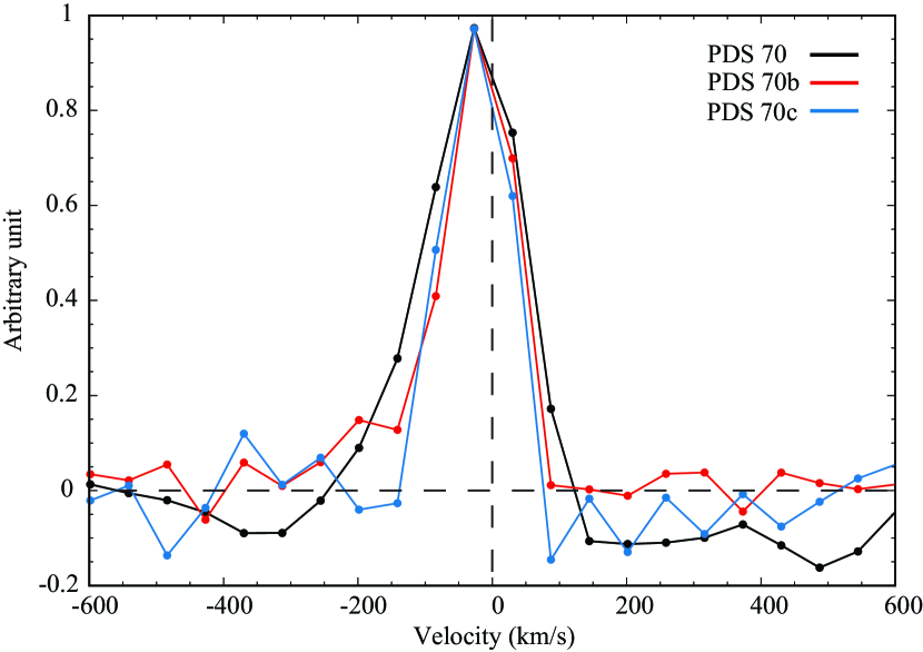
Figure 2: Normalized H$\alpha$ line profiles of PDS 70 and its two planets. The planetary H$\alpha$ data are the same as those in Figure 1, but are normalized. The vertical dotted line represents the rest wavelength of H$\alpha$ at 6562.8 Å.

4 Physical Properties of Accreting Planets

4.1 Free-fall Velocity of Gas and Pre-shock Number Density of Hydrogen Nuclei

The simultaneous observations of H$\alpha$ and H$\beta$ with MUSE provide reliable measurements of the line flux ratio without any concerns regarding the temporal variability of each flux. Signals of H$\beta$ emissions are not seen in both PDS 70b and c, and we only obtained the upper limit of its flux. However, the upper limit of H$\beta$ emissions allows us to constrain the physical parameters related to the planetary accretion. Following the method in Aoyama & Ikoma (2019), we first estimated the free-fall velocity $v_{0}$ of the gas and the pre-shock number density of hydrogen nuclei $n_{0}$ using the accretion shock model in Aoyama et al. (2018). Here, we assume that the accretion speed is the same as the free-fall velocity. The observational constraints for these quantities are given by the H$\alpha$ linewidths at 10 % and 50 % maxima (Table 1). As explained in Aoyama & Ikoma (2019), the H$\alpha$ linewidth increases with $n_{0}$ and $v_{0}$. This is because an increase of $n_{0}$ enhances absorption of H$\alpha$ emissions near the line center by shock-heated gas, while a high value of $v_{0}$ means that a flow with higher velocity passes. Thus the H$\alpha$ linewidth is a function of $n_{0}$ and $v_{0}$ (see Figure 5 in Aoyama & Ikoma, 2019). In Figure 3, the intersections of the H$\alpha$ 10 % & 50 % linewidths indicate that ($v_{0}$, $n_{0}$) is roughly ($144$ km s^-1, $3.8\times 10^{13}$ cm^-3) and ($139$ km s^-1, $3.2\times 10^{13}$ cm^-3) for PDS 70b and c, respectively.

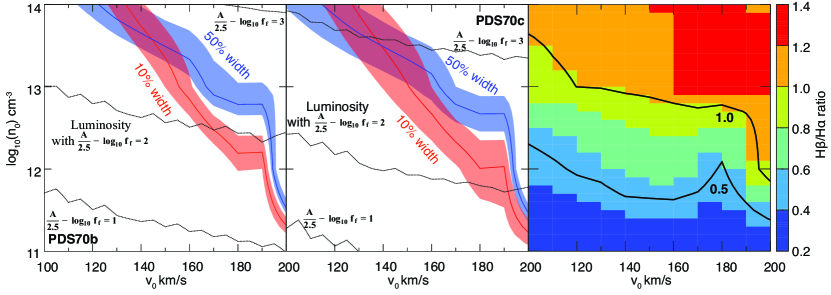
Figure 3: Model input parameters $v_{0}\,\mathrm{km/s}$ and $n_{0}\,\mathrm{cm^{-3}}$ reproducing the H$\alpha$ line profile observed in PDS 70b (left) and c (center). The red and blue lines correspond to the H$\alpha$ linewidth at 10 % and 50 % of maximum flux, respectively. The colored shades show their 1 $\sigma$ errors taken from fitting errors in Table 1. The black dotted lines show the dereddened line luminosity for the planetary radius of $2R_{\mathrm{J}}$ and different filling factors $f_{\mathrm{f}}$. The cross points of the red and blue lines roughly indicate $(v_{0},~{}n_{0})=(144~{}\mathrm{km/s},~{}3.8\times 10^{13}~{}\mathrm{cm^{-3}})$ and $(139~{}\mathrm{km/s},~{}3.2\times 10^{13}~{}\mathrm{cm^{-6}})$ for PDS70b and c, respectively. To reproduce the dereddened luminosity at these cross points, the values of $10^{A/2.5}/f_{\mathrm{f}}$ are estimated to be $5\times 10^{2}$ and $9\times 10^{2}$, respectively. Note that the values of $A_{H\alpha}$ used here are 2.0 and 1.1 mag for PDS 70b and c, respectively (§ 4.2). The right panel shows the ratio of H$\beta$ to H$\alpha$. The cross points in the left and middle panels indicate that the flux ratio is close to unity for PDS 70b and c.

4.2 Line Flux Ratio and Extinction

The theoretical model of Aoyama & Ikoma (2019) suggests that the flux ratio of H$\beta$ to H$\alpha$ ($F_{\rm H\beta}/F_{\rm H\alpha}$) increases with $n_{0}$ when there is no foreground extinction, e.g., interstellar extinction (right panel in Figure 3). This is because the higher density of $n_{0}\gtrsim$ 10¹³ cm^-3 is large enough to saturate the H$\alpha$ flux due to the effect of absorption in the post-shock region. Meanwhile, since the emission source for H$\beta$ is more excited than that for H$\alpha$, higher values of $v_{0}$ or $n_{0}$ are necessary to put H$\beta$ in such a saturated state (see Aoyama et al., 2018 for more details). Hence the value of $F_{\rm H\beta}$/$F_{\rm H\alpha}$ is close to unity for $n_{0}\gtrsim$ 10¹³ cm^-3. In contrast, a H$\alpha$ absorption is negligible with the lower density of $n_{0}\lesssim$ 10¹² cm^-3, resulting in a smaller value of $F_{\rm H\beta}/F_{\rm H\alpha}\lesssim$ 0.5.

With values of $n_{0}$ and $v_{0}$ as derived above for PDS 70b and c, the theoretical value of the flux ratio is close to unity (right panel in Figure 3). However, our observed values of $F_{\rm H\beta}$/$F_{\rm H\alpha}$ at a 3-$\sigma$ upper limit for PDS 70b and c are $<$ 0.28 and $<$ 0.52, respectively, which are smaller than the theoretically expected values. These observed values are also similar with accreting T Tauri stars and brown dwarfs with the values of 0.1–0.5 (see Table 7 in Herczeg & Hillenbrand, 2008). This underestimating of the flux ratio could be due to extinction of circumplanetary materials. According to ALMA observations and numerical simulations by Keppler et al. (2019), gas is likely to exist in the dust gap of the circumstellar disk where PDS 70b and c are located. We conjecture that small dust grains (sub-micron size) are well coupled with gas in the gap, contributing to the extinction. Based on this speculation, we use the extinction law $A_{\lambda}\propto\lambda^{-1.75}$ (Draine, 1989) to estimate the extinction. Considering the theoretical prediction that the value of $F_{\rm H\beta}$/$F_{\rm H\alpha}$ without extinction is unity, we derived $A_{H\alpha}>$ 2.0 and $>$ 1.1 mag for PDS 70b and c, respectively. We note that the extinction law is valid in the range $0.7\lesssim\lambda\lesssim 5\mu$m, and the slope of extinction will be gentle at H$\alpha$ and H$\beta$ wavelengths (see Figure 1 in Draine, 1989). The gentle slope will make the lower limit of $A_{H\alpha}$ larger than the above value.

4.3 Filling Factor, Planetary Mass, and Mass Accretion Rate

We estimate the filling factor $f_{\mathrm{f}}$ using the following equation for the H$\alpha$ luminosity (Aoyama & Ikoma, 2019):

$$L_{\rm H_{\alpha}}=4\pi R_{\rm p}^{2}f_{\mathrm{f}}I_{\rm H_{\alpha}}10^{-0.4A_{\rm H_{\alpha}}},$$ (1)

or

$$0.4A_{\rm H_{\alpha}}-\log_{10}f_{\mathrm{f}}=-\log_{10}L_{\rm H_{\alpha}}+\log_{10}(4\pi R_{\rm p}^{2}I_{\rm H_{\alpha}}),$$ (2)

where $R_{\rm p}$ and $I_{\rm H_{\alpha}}$ are the planetary radius and the H$\alpha$ energy flux per unit area, respectively. The H$\alpha$ luminosities are calculated from the line fluxes listed in Table 1. We assume that the planetary radius $R_{\rm p}$ is $2R_{\rm Jup}$, where $R_{\rm Jup}$ is the Jovian radius (Spiegel & Burrows, 2012). $I_{\rm H_{\alpha}}$ is a function of $n_{0}$ and $v_{0}$, and its dependence is investigated in Aoyama et al. (2018). Using these results, we plot the lines of $0.4A_{\rm H_{\alpha}}-\log_{10}f_{\mathrm{f}}$ with different values in the $v_{0}$–$n_{0}$ plane (left and middle panels in Figure 3). The lower limits for the extinction $A_{H\alpha}$ constrain the possible range of the filling factor: $A_{H\alpha}>$ 2.0 and $>$ 1.1 mag give $f_{\mathrm{f}}\gtrsim 0.01$ and $\gtrsim 0.003$ for PDS 70b and c, respectively.

We can also derive a planetary dynamical mass $M_{\mathrm{P}}$ and an accretion rate $\dot{M}_{\mathrm{P}}$ (Aoyama & Ikoma, 2019), written as

$$M_{\mathrm{P}} = \frac{R_{\mathrm{P}}v_{0}^{2}}{2G}~{}\mathrm{and}$$ (3)

$$\dot{M}_{\mathrm{P}} = \mu n_{0}v_{0}f_{\mathrm{f}}(4\pi R_{\mathrm{P}}^{2}),$$ (4)

respectively, where $G$ is the gravitational constant and $\mu$ is the mean mass per hydrogen nucleus. Using $\mu=2.3\times 10^{-24}$ g and $R_{\rm P}=$ 2 $R_{\rm Jup}$, we estimate $M_{\mathrm{P}}$ of 12 $\pm$ 3 $M_{\rm Jup}$ and $\dot{M}_{\mathrm{P}}\gtrsim$ 5$\times 10^{-7}\,M_{\mathrm{Jup}}\,\mathrm{yr^{-1}}$ for PDS 70b, and $M_{\mathrm{P}}$ of 11 $\pm$ 5 $M_{\rm Jup}$ and $\dot{M}_{\mathrm{P}}\gtrsim$ 1$\times 10^{-7}\,M_{\mathrm{Jup}}\,\mathrm{yr^{-1}}$ for PDS 70c.

5 Discussion

5.1 Planetary Mass

The planetary mass is commonly estimated by comparing photometric and spectroscopic observations with planetary evolution and atmospheric models (e.g., Müller et al., 2018; Keppler et al., 2018; Christiaens et al., 2019a; Haffert et al., 2019; Mesa et al., 2019). On the other hand, our method based on the accretion shock model can estimate a dynamic planetary mass (Aoyama & Ikoma, 2019). In § 4.3, we estimated the masses of PDS 70b and c to be $\sim$12 and $\sim$11 $M_{\rm Jup}$, respectively. As shown in eq. 3, these values depend on the planetary radii, which cannot be constrained only by MUSE observations. We consider the possible range of the planetary radii suggested by the planetary evolution model, which predicts the radii to be $\sim$1–2 $R_{\rm Jup}$ with an age of $\lesssim 10$ Myr (Spiegel & Burrows, 2012). Therefore, the planetary mass derived from the radii of $2R_{\rm Jup}$ will give the upper limit. We also note that the observed linewidths will be the upper limits, because the linewidths of the two planets are similar to MUSE’s spectral resolution, $\sim$120 km s^-1. Our estimated masses are consistent with previous near-infrared photometric and spectroscopic estimations: the mass of PDS 70b is estimated to be 5–9 and 2–17 $M_{\rm Jup}$ from photometric and spectroscopic observations, respectively (Keppler et al., 2018; Müller et al., 2018), while PDS 70c’s mass is 4–12 $M_{\rm Jup}$ from photometric observations (Haffert et al., 2019; Mesa et al., 2019). Our mass estimation method is independent of the previous methods based on the planetary evolution and atmospheric models only, and therefore will provide a powerful tool to calibrate these models.

5.2 Origin of Planetary Extinction

The extinction of the primary star was found to be negligible (Müller et al., 2018). However, our observations suggest that PDS 70b and c have $A_{\rm H\alpha}>$ 2.0 and $>$ 1.1 mag, respectively. We hypothesize that small (sub-micron size) grains coupled with the gas in the dust gap in the circumstellar disk is the cause of the planetary extinction. Such dust, if it exists, will not be clearly visible in existing observations because of their faintness. Here, we estimate the contribution of the unseen dust to the extinction. Keppler et al. (2019) conducted hydrodynamic simulations to reproduce the observed ¹²CO (2–1) integrated intensity map and found that the azimuthally averaged gas surface density at the location of PDS 70b is $\sim$0.01 g cm^-2, which can be translated to a molecular hydrogen surface density of $\sim$3 $\times$ 10²¹ cm^-2. By using the relationship between the interstellar dust extinction and the hydrogen column density ($N_{\rm H}$/$A_{V}=1.9\times 10^{21}$ cm^-2 mag^-1; Bohlin et al., 1978), we derived $A_{V}\sim$ 3.3 mag, which corresponds to $A_{H\alpha}$ $\sim$ 2.4 mag with $A_{\lambda}\propto\lambda^{-1.75}$ (Draine, 1989), where we assume that hydrogen atoms are in the form of hydrogen molecules. The derived vertical extinction at the gap region is comparable to the planetary extinction estimated by the accretion shock model, which supports our idea that the origin of extinction is small, unseen dust grains in the gap.

5.3 Planetary Mass Accretion Rate

We now consider the influence of the extinction on the estimation of the mass accretion rate. First, we briefly explain the relationship between the extinction and the mass accretion rate. As shown in eq. 4, the mass accretion rate is a function of $f_{\mathrm{f}}$, $n_{0}$, and $v_{0}$. The values of $n_{0}$ and $v_{0}$ can be estimated from the H$\alpha$ linewidths (left and middle panels in Figure 3), and hence we only need to estimate the value of $f_{\mathrm{f}}$. This value can be estimated from eq. 1, with the free parameter $A_{\rm H\alpha}$. The value of $A_{\rm H\alpha}$ was independently estimated from the line ratio (right panel in Figure 3). For PDS 70b, we derived an H$\alpha$ extinction of $A_{\rm H\alpha}>$ 2.0 mag in the pre-shock region (§ 4.2). With eq. 1 and 4, the value of the mass accretion rate derived from the dereddened luminosity is $\dot{M}_{\mathrm{P}}\gtrsim$ 5 $\times$ 10^-7 $M_{\rm Jup}$ yr^-1 (left panel in Figure 3). The PDS 70c mass accretion rate was revised to $\gtrsim$ 1 $\times$ 10^-7 $M_{\rm Jup}$ yr^-1 with $A_{\rm H\alpha}>$ 1.1 mag (middle panel in Figure 3). Note that our estimation of the mass accretion rate in this paper is limited by the detection limit of the H$\beta$ flux, and the true mass accretion rate should be higher than the current values. In particular, we speculate that the intrinsic mass accretion rate of PDS 70c is larger than that of PDS 70b because the infrared color of $K1$–$L^{\prime}$ in PDS 70c with $\sim$2.2 mag is redder than that of PDS 70b with $\sim$1.1 mag (Haffert et al., 2019), resulting in a much larger value of $A_{\rm H\alpha}$ for PDS 70c. To better constrain the mass accretion rate of PDS 70b and c, deep multiple-line observations with less extinction, such as Pa$\beta$ (1.282 $\mu$m) and Br$\gamma$ (2.166 $\mu$m), are preferable.

Our analysis suggests that the mass accretion rates of PDS 70b and c are $\gtrsim$ 8$\times$ and $\gtrsim$ 2$\times$ higher than that of the primary star ($\sim$6 $\times$ 10^-8 $M_{\rm Jup}$ yr^-1; Haffert et al., 2019). Recently, Thanathibodee et al. (2020) applied magnetospheric accretion models to the H$\alpha$ line profile of PDS 70 and derived mass accretion rates onto the star in the range of 0.6–2.2 $\times$ 10^-7 $M_{\rm Jup}$ yr^-1. Even with these new stellar values, the mass accretion rate of PDS 70b is still higher. Since the number of accreting planets embedded in the protoplanetary disk is currently believed to be three (LkCa 15b, PDS 70b, and PDS 70c; Kraus & Ireland, 2012; Sallum et al., 2015; Wagner et al., 2018; Haffert et al., 2019), it is uncertain whether this situation (i.e., a higher planetary accretion rate) is common or rare. Numerical simulations predict that the mass accretion rate of a 1-$M_{\rm Jup}$ planet can reach up to $\sim$90 % of the gas flow from the outer disk (Lubow & D’Angelo, 2006). Furthermore, Tanigawa & Tanaka (2016) showed that the mass accretion rate of a planet in the gas gap of the disk can exceed the stellar mass accretion rate in the case of a lower planetary mass and/or a higher gas scale height (see eq. 16 in Tanigawa & Tanaka, 2016). Therefore, a situation similar to the PDS 70 system can occur at a certain evolution phase in other disk systems.

Additionally we compared our results with the mass accretion rates of other young planetary-mass companions (GSC 06214–0210b, GQ Lup b, DH Tau b, and SR 12c in Bowler et al., 2011; Zhou et al., 2014; Santamaría-Miranda et al., 2018). The mass accretion rate of GQ Lup b ($\dot{M}_{\mathrm{P}}\sim$ 5 $\times$ 10^-7 $M_{\rm Jup}$ yr^-1; Zhou et al., 2014) is comparable with that of PDS 70b, while other three objects have lower values by a few orders of magnitude ($\dot{M}_{\mathrm{P}}\sim$ 10^-9–10^-8 $M_{\rm Jup}$ yr^-1; Bowler et al., 2011; Zhou et al., 2014; Santamaría-Miranda et al., 2018). These results of the higher mass accretion rates of PDS 70b and GQ Lup b could be naturally explained by the fact that these two are embedded in the circumstellar disk (Keppler et al., 2019; MacGregor et al., 2017) and can be supplied with a fresh disk material from the parent disk.

5.4 Accretion Process

Our analysis based on the accretion shock model suggests that $f_{\mathrm{f}}\sim 10^{-2}$–10^-3 for PDS 70b and c. If the H$\alpha$ emitting regions are actually accretion shock regions, the accretion flow toward the protoplanets should be significantly converged by some mechanisms. The existence of accretion shocks by converging flows has been suggested for pre-main-sequence stars such as classical T-Tauri stars, where strong stellar magnetic fields guide and collimate the accretion flows toward the magnetic poles (Koenigl, 1991; Hartmann et al., 2016). The very small filling factors for PDS 70b and c may imply that magnetospheric accretion operates even in these protoplanets (for recent theoretical studies, see Batygin, 2018; Thanathibodee et al., 2019). However, the existence of sufficiently strong planetary magnetic fields remains unclear, and needs to be examined observationally (e.g., radio observations with a low frequency of 10s of MHz are currently being performed: Zarka et al., 2019). If there are no magnetic fields or only a weak field in PDS 70b and c, some hydrodynamic processes should be responsible for collimating the accretion flows.

When a protoplanet does not develop a magnetosphere due to it having a weak magnetic field, and its circumplanetary disk extends to the planetary surface, the boundary layer between the protoplanet and the disk is heated due to a viscous process and can be a source of H$\alpha$ emissions. Boundary layer accretion has also been considered for pre-main-sequence stars (Bertout et al., 1988). Further theoretical and observational studies are required to identify the accretion processes. For example, high spectral resolution observations to search for the inverse P Cygni profile will help to investigate the possibility of magnetospheric accretion (e.g., AA Tau; Edwards et al., 1994). Observational investigations of planetary magnetic fields at radio wavelengths will give constraints on the field strength (e.g., SKA: the Square Kilometre Array; Zarka et al., 2015). Multi-epoch observations of accreting signatures at optical/NIR wavelengths (e.g., VLT/MUSE or Keck/OSIRIS) will provide the information on time-variability; magnetospheric accretion in pre-main-sequence stars commonly show time-variability (e.g., Cody & Hillenbrand, 2014).

6 Summary

We re-analyzed MUSE archive data obtained with commissioning observations, and estimated the upper limit of H$\beta$ emissions for PDS 70b. Most of the observational results are similar to those of previous studies in Haffert et al. (2019). The main difference is the planetary mass accretion rate. We derived the accretion properties of PDS 70b by assuming that the H$\alpha$ emissions originate from gas accretion shock. We showed that the line flux ratio $F_{\rm H\beta}$/$F_{\rm H\alpha}$ is useful to constrain the planetary mass accretion rate by estimating the extinction of $A_{H\alpha}$ because the accretion rate is described as a function of $A_{H\alpha}$. The 3-$\sigma$ upper limit of $F_{\rm H\beta}$/$F_{\rm H\alpha}=$ 0.28 can be translated to $A_{H\alpha}>$ 2.0 mag. We then obtained a value for dereddened $F_{\rm H\alpha}>$ 5 $\times$ 10^-15 erg s^-1 cm^-2. With the H$\alpha$ linewidth and the dereddened H$\alpha$ line luminosity for PDS 70b, we derived a mass accretion rate of $\dot{M}\gtrsim$ 5 $\times$ 10^-7 $M_{\rm Jup}$ yr^-1 for PDS 70b. PDS 70b’s mass accretion rate is an order of magnitude larger than that of PDS 70 with $\dot{M}\sim$ 6 $\times$ 10^-8 $M_{\rm Jup}$ yr^-1. We also derived a filling factor $f_{\rm f}$ of $\gtrsim$ 0.01 for PDS 70b. This result suggests that the H$\alpha$ emitting areas are localized at the surface of PDS 70b. Multiple line observations, especially emission lines with low extinction, such as Pa$\beta$ (1.282 $\mu$m) and Pa$\delta$ (2.166 $\mu$m), are useful for determining better constraints on the planetary accretion properties of young planets deeply embedded in molecular clouds or circumstellar disks.

Figure 5 shows different spectra in the stellar and halo regions, which is corrected in § 2.2.

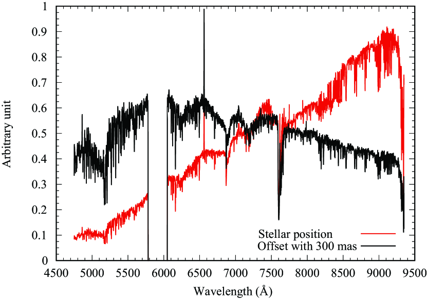
Figure 5: Spectra in the 3 $\times$ 3 pixels area at the stellar position (red) and at the halo region with a 300-mas offset from the stellar position (black). Since adaptive optics systems work well at longer wavelengths, the flux in the arbitrary box at the stellar position is brighter at longer wavelengths.

Figure 6 shows each spectrum in the procedure of correcting the fake continuum pattern in § 2.2.

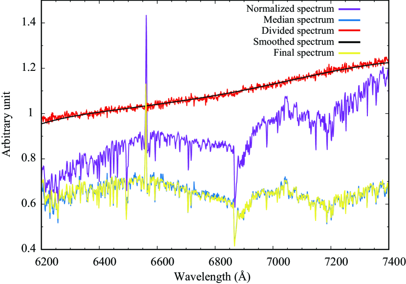
Figure 6: Stepwise correction of the fake continuum pattern in each spatial pixel. A purple line is a spectrum of each spatial pixel normalized by a median spectrum of 9,600 spectra (a blue line). A red spectrum represents that the purple spectrum is divided by the blue one. A black line is a Gaussian smoothed spectrum of the red divided one. A yellow line is a final spectrum in which the purple normlized spectrum is divided by the black smoothed one. All spectra are normalized and offset for the presentation purpose.

References

- Aoyama & Ikoma (2019) Aoyama, Y., & Ikoma, M. 2019, ApJ, 885, L29, doi: 10.3847/2041-8213/ab5062
- Aoyama et al. (2018) Aoyama, Y., Ikoma, M., & Tanigawa, T. 2018, ApJ, 866, 84, doi: 10.3847/1538-4357/aadc11
- Bacon et al. (2010) Bacon, R., Accardo, M., Adjali, L., et al. 2010, in Society of Photo-Optical Instrumentation Engineers (SPIE) Conference Series, Vol. 7735, Proc. SPIE, 773508
- Batygin (2018) Batygin, K. 2018, The Astronomical Journal, 155, 178, doi: 10.3847/1538-3881/aab54e
- Bertout et al. (1988) Bertout, C., Basri, G., & Bouvier, J. 1988, ApJ, 330, 350, doi: 10.1086/166476
- Bohlin et al. (1978) Bohlin, R. C., Savage, B. D., & Drake, J. F. 1978, ApJ, 224, 132, doi: 10.1086/156357
- Bowler et al. (2011) Bowler, B. P., Liu, M. C., Kraus, A. L., Mann, A. W., & Ireland, M. J. 2011, ApJ, 743, 148, doi: 10.1088/0004-637X/743/2/148
- Calvet & Gullbring (1998) Calvet, N., & Gullbring, E. 1998, The Astrophysical Journal, 509, 802, doi: 10.1086/306527
- Christiaens et al. (2019a) Christiaens, V., Cantalloube, F., Casassus, S., et al. 2019a, ApJ, 877, L33, doi: 10.3847/2041-8213/ab212b
- Christiaens et al. (2019b) Christiaens, V., Casassus, S., Absil, O., et al. 2019b, MNRAS, 486, 5819, doi: 10.1093/mnras/stz1232
- Cody & Hillenbrand (2014) Cody, A. M., & Hillenbrand, L. A. 2014, ApJ, 796, 129, doi: 10.1088/0004-637X/796/2/129
- Draine (1989) Draine, B. T. 1989, in Infrared Spectroscopy in Astronomy, ed. E. Böhm-Vitense, 93
- Edwards et al. (1994) Edwards, S., Hartigan, P., Ghandour, L., & Andrulis, C. 1994, AJ, 108, 1056, doi: 10.1086/117134
- Freudling et al. (2013) Freudling, W., Romaniello, M., Bramich, D. M., et al. 2013, A&A, 559, A96, doi: 10.1051/0004-6361/201322494
- Gaia Collaboration et al. (2018) Gaia Collaboration, Brown, A. G. A., Vallenari, A., et al. 2018, A&A, 616, A1, doi: 10.1051/0004-6361/201833051
- Haffert et al. (2019) Haffert, S. Y., Bohn, A. J., de Boer, J., et al. 2019, Nature Astronomy, 329, doi: 10.1038/s41550-019-0780-5
- Hartmann et al. (2016) Hartmann, L., Herczeg, G., & Calvet, N. 2016, ARA&A, 54, 135, doi: 10.1146/annurev-astro-081915-023347
- Hayashi et al. (1985) Hayashi, C., Nakazawa, K., & Nakagawa, Y. 1985, in Protostars and Planets II, ed. D. C. Black & M. S. Matthews, 1100–1153
- Henden et al. (2015) Henden, A. A., Levine, S., Terrell, D., & Welch, D. L. 2015, in American Astronomical Society Meeting Abstracts, Vol. 225, American Astronomical Society Meeting Abstracts #225, 336.16
- Herczeg & Hillenbrand (2008) Herczeg, G. J., & Hillenbrand, L. A. 2008, ApJ, 681, 594, doi: 10.1086/586728
- Howell (1990) Howell, S. B. 1990, in Astronomical Society of the Pacific Conference Series, Vol. 8, CCDs in astronomy, ed. G. H. Jacoby, 312–318
- Ida & Lin (2004) Ida, S., & Lin, D. N. C. 2004, ApJ, 604, 388, doi: 10.1086/381724
- Isella et al. (2019) Isella, A., Benisty, M., Teague, R., et al. 2019, ApJ, 879, L25, doi: 10.3847/2041-8213/ab2a12
- Jee et al. (2007) Jee, M. J., Blakeslee, J. P., Sirianni, M., et al. 2007, PASP, 119, 1403, doi: 10.1086/524849
- Kamp & Dullemond (2004) Kamp, I., & Dullemond, C. P. 2004, ApJ, 615, 991, doi: 10.1086/424703
- Keppler et al. (2018) Keppler, M., Benisty, M., Müller, A., et al. 2018, A&A, 617, A44, doi: 10.1051/0004-6361/201832957
- Keppler et al. (2019) Keppler, M., Teague, R., Bae, J., et al. 2019, A&A, 625, A118, doi: 10.1051/0004-6361/201935034
- Koenigl (1991) Koenigl, A. 1991, ApJ, 370, L39, doi: 10.1086/185972
- Kraus & Ireland (2012) Kraus, A. L., & Ireland, M. J. 2012, ApJ, 745, 5, doi: 10.1088/0004-637X/745/1/5
- Lubow & D’Angelo (2006) Lubow, S. H., & D’Angelo, G. 2006, ApJ, 641, 526, doi: 10.1086/500356
- Lubow et al. (1999) Lubow, S. H., Seibert, M., & Artymowicz, P. 1999, ApJ, 526, 1001, doi: 10.1086/308045
- MacGregor et al. (2017) MacGregor, M. A., Wilner, D. J., Czekala, I., et al. 2017, ApJ, 835, 17, doi: 10.3847/1538-4357/835/1/17
- Mesa et al. (2019) Mesa, D., Keppler, M., Cantalloube, F., et al. 2019, A&A, 632, A25, doi: 10.1051/0004-6361/201936764
- Müller et al. (2018) Müller, A., Keppler, M., Henning, T., et al. 2018, A&A, 617, L2, doi: 10.1051/0004-6361/201833584
- Pecaut & Mamajek (2016) Pecaut, M. J., & Mamajek, E. E. 2016, MNRAS, 461, 794, doi: 10.1093/mnras/stw1300
- Popham et al. (1993) Popham, R., Narayan, R., Hartmann, L., & Kenyon, S. 1993, ApJ, 415, L127, doi: 10.1086/187049
- Sallum et al. (2015) Sallum, S., Follette, K. B., Eisner, J. A., et al. 2015, Nature, 527, 342, doi: 10.1038/nature15761
- Santamaría-Miranda et al. (2018) Santamaría-Miranda, A., Cáceres, C., Schreiber, M. R., et al. 2018, Monthly Notices of the Royal Astronomical Society, 475, 2994, doi: 10.1093/mnras/stx3325
- Spiegel & Burrows (2012) Spiegel, D. S., & Burrows, A. 2012, ApJ, 745, 174, doi: 10.1088/0004-637X/745/2/174
- Suzuki et al. (2018) Suzuki, D., Bennett, D. P., Ida, S., et al. 2018, ApJ, 869, L34, doi: 10.3847/2041-8213/aaf577
- Tanigawa & Ikoma (2007) Tanigawa, T., & Ikoma, M. 2007, apj, 667, 557, doi: 10.1086/520499
- Tanigawa et al. (2012) Tanigawa, T., Ohtsuki, K., & Machida, M. N. 2012, ApJ, 747, 47, doi: 10.1088/0004-637X/747/1/47
- Tanigawa & Tanaka (2016) Tanigawa, T., & Tanaka, H. 2016, ApJ, 823, 48, doi: 10.3847/0004-637X/823/1/48
- Thanathibodee et al. (2019) Thanathibodee, T., Calvet, N., Bae, J., Muzerolle, J., & Hernández, R. F. 2019, ApJ, 885, 94, doi: 10.3847/1538-4357/ab44c1
- Thanathibodee et al. (2020) Thanathibodee, T., Molina, B., Calvet, N., et al. 2020, arXiv e-prints, arXiv:2002.07283. https://arxiv.org/abs/2002.07283
- Wagner et al. (2018) Wagner, K., Follete, K. B., Close, L. M., et al. 2018, ApJ, 863, L8, doi: 10.3847/2041-8213/aad695
- Weilbacher et al. (2012) Weilbacher, P. M., Streicher, O., Urrutia, T., et al. 2012, Society of Photo-Optical Instrumentation Engineers (SPIE) Conference Series, Vol. 8451, Design and capabilities of the MUSE data reduction software and pipeline, 84510B
- Zarka et al. (2015) Zarka, P., Lazio, J., & Hallinan, G. 2015, in Advancing Astrophysics with the Square Kilometre Array (AASKA14), 120
- Zarka et al. (2019) Zarka, P., Li, D., Grießmeier, J.-M., et al. 2019, Research in Astronomy and Astrophysics, 19, 023, doi: 10.1088/1674-4527/19/2/23
- Zhou et al. (2014) Zhou, Y., Herczeg, G. J., Kraus, A. L., Metchev, S., & Cruz, K. L. 2014, The Astrophysical Journal, 783, L17, doi: 10.1088/2041-8205/783/1/L17
- Zhu (2015) Zhu, Z. 2015, ApJ, 799, 16, doi: 10.1088/0004-637X/799/1/16