The Value of Nullspace Tuning Using Partial Label Information

Abstract

In semi-supervised learning, information from unlabeled examples is used to improve the model learned from labeled examples. But in some learning problems, partial label information can be inferred from otherwise unlabeled examples and used to further improve the model. In particular, partial label information exists when subsets of training examples are known to have the same label, even though the label itself is missing. By encouraging a model to give the same label to all such examples, we can potentially improve its performance. We call this encouragement Nullspace Tuning because the difference vector between any pair of examples with the same label should lie in the nullspace of a linear model. In this paper, we investigate the benefit of using partial label information using a careful comparison framework over well-characterized public datasets. We show that the additional information provided by partial labels reduces test error over good semi-supervised methods usually by a factor of 2, up to a factor of 5.5 in the best case. We also show that adding Nullspace Tuning to the newer and state-of-the-art MixMatch method decreases its test error by up to a factor of 1.8.

1 Introduction

Semi-supervised learning methods attempt to improve a model learned from labeled examples by using information extracted from unlabeled examples (Chapelle et al., 2006; Zhu et al., 2003; Verma et al., 2019). One effective approach is to use some form of data augmentation, in which a new example is created by transforming an unlabeled example (Cubuk et al., 2019; Berthelot et al., 2019), and then encouraging the model to predict the same label for both.

In some learning problems, we already know that some unlabeled examples have the same label, even though that label is missing. For example, we may know that multiple photos are of the same object because of the way the photos were acquired, despite not having a label for that object. In the medical domain, repeated imaging of the same patient is common (Yankelevitz et al., 1999; Freeborough & Fox, 1997; Dirix et al., 2009), and if the learning task is to predict something that does not change over time (or at least not over the short time between images), then we know that the repeated images have the same label. We call this knowledge partial label information, and distinguish it from the standard semi-supervised assumption that there is no label information at all for the unlabeled examples.

In prior work, Nath (2018) used partial label information to predict fiber orientation distributions in magnetic resonance imaging, and Huo (2019) used it for coronary artery calcium detection in non-contrast computed tomography scans. But there has been no careful investigation of how much the partial label information can add to a model’s performance. In this paper, we evaluate the performance benefit of partial labels using the rigorous, standardized approach described by Oliver (2018), which is designed to realistically assess the relative performance of semi-supervised learning approaches.

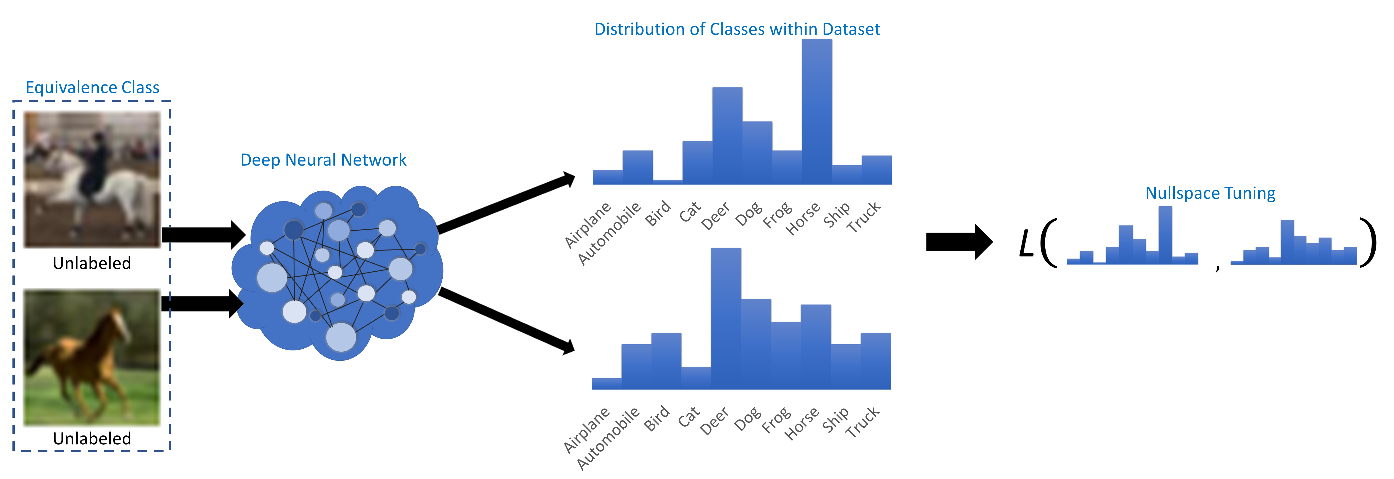
Figure 1: With two unlabeled images in a equivalency class in the class ”Horse” from the CIFAR-10 dataset, NST constrains the network by adding a loss term which penalizes differences in the resulting probability distributions.

In this work, we use the term equivalence class to indicate a subset of unlabeled examples for which the label is known to be the same. An equivalence class need not contain all of the examples with the same label. Formally, an equivalence class $Q$ of examples $x$ in a data subset $D$ under a true but unknown labeling function $f$ is defined as:

$$Q=\{x\in D|f(x)=c\},$$ (1)

where $c$ is a constant. If we know that a particular pair $x_{1},x_{2}\in Q$, we express this as $x_{1}\sim x_{2}$.

If the labeling function $f$ is a linear operator, then the difference between any two examples in $Q$ lies in the nullspace of $f$:

$$f(x_{1})=f(x_{2})\iff f(x_{1}-x_{2})=0.$$ (2)

Because the term nullspace is so evocative, we abuse it here to conceptually refer to comparisons between elements of the sets defined by (1), even though for a nonlinear function $f$ the relationship (2) does not hold.

We can use our knowledge of the natural equivalence classes in a dataset to help tune a model using a procedure that we call Nullspace Tuning, in which the model is encouraged to label examples $x_{1}$ and $x_{2}$ the same when $x_{1}\sim x_{2}$. Nullspace tuning is easily implemented by adding a term to the loss function to penalize the difference in label probabilities $h(x_{1})-h(x_{2})$ assigned by the current model $h$ when $x_{1}\sim x_{2}$. (Figure 1).

Nullspace Tuning is related to the idea of Data Augmentation (see Section 2.1 below). Data Augmentation is used when we know specific transformations that should not affect the label, and we create new training examples by transforming existing examples and keeping the label constant, whether that label is known or unknown. This implicitly places those transformations into the architecture’s nullspace. In contrast, Nullspace Tuning explicitly places naturally occurring but unknown transformations into the nullspace when nature provides examples of them by way of partial labels. Of course, the two approaches can be used together, which we also demonstrate in this paper.

2 Related Work

Data augmentation, semi-supervised learning, and dual and triplet networks are existing learning approaches that are closely related to Nullspace Tuning, and there is a large literature for each. Thorough reviews are available elsewhere (Perez & Wang, 2017; Zhu & Goldberg, 2009; Zhu, 2005; Kumar et al., 2016). In this section we discuss specific work that is most closely related, and work that we use as experimental baselines.

2.1 Data Augmentation

Data Augmentation artificially expands a training dataset by modifying examples using transformations that are believed not to affect the label. Image deformations and additive noise are common examples of such transformations (Cireşan et al., 2010; Cubuk et al., 2019; Simard et al., 2003). The most effective data augmentations may be specific to the learning task or dataset and driven by domain knowledge. Elastic distortions, scale, translation, and rotation are used in the majority of top performing MNIST models (Wan et al., 2013; Sato et al., 2015; Simard et al., 2003; Ciregan et al., 2012). Random cropping, mirroring, and color shifting are often used to augment natural images (Krizhevsky et al., 2012). Recent work automatically selects effective data augmentation policies from a search space of image processing functions (Cubuk et al., 2019).

2.2 Equivalence Classes in Labeled Data

An idea similar to Nullspace Tuning was used by Bromley (1994) in fully supervised learning, where $x_{1}\sim x_{2}$ is known because their labels are observed. They used this fact to improve a signature verification model by minimizing distance between different signatures from the same person, essentially tuning the nullspace of the network with labeled equivalence classes. This idea later inspired triplet networks (Schroff et al., 2015) that learn from tuples $(x,x^{+},x^{-})$, where $x\sim x^{+}$ and $x\nsim x^{-}$, and the predicted probabilities are encouraged in the loss function to be respectively near or far. There are also multiple works that indicate usage of Siamese networks for person re-identification (McLaughlin et al., 2016; Chung et al., 2017; Varior et al., 2016). Nullspace Tuning extends these ideas to the case where the labels are missing but still known to be the same.

2.3 Semi-supervised Learning

Recent approaches to Semi-supervised Learning add to the loss function a term computed over unlabeled data that encourages the model to generalize more effectively. There are many examples of this, but we describe those here that we use for comparison in our experiments.

$\Pi$-Model encourages consistency between multiple predictions of the same example under the perturbations of data augmentation or dropout. The loss term penalizes the distance between the model’s prediction of two perturbations of the same sample (Laine & Aila, 2016; Sajjadi et al., 2016).

Mean Teacher builds on $\Pi$-Model by stabilizing the target for unlabeled samples. The target for unlabeled samples is generated from a teacher model using the exponential moving average of the student model’s weights. This allows information to be aggregated after every step rather than after every epoch (Tarvainen & Valpola, 2017).

Virtual Adversarial Training (VAT) approximates a tiny perturbation which, if added to unlabeled sample $x$, would most significantly change the resulting prediction without altering the underlying class (Miyato et al., 2018). VAT can be used in place of or in addition to data augmentation, and is not domain specific.

Pseudo-labeling uses the prediction function to repeatedly update the class probabilities for an unlabeled sample during training. Probabilities that are higher than some selected threshold are treated as targets in the loss function, but typically the unlabeled portion of the loss is regulated by another hyperparameter (Lee, 2013).

MixUp creates augmented data by forming linear interpolations between examples. If the two source examples have different labels, the new label is also an interpolation of the two (Zhang et al., 2017).

MixMatch was developed by taking key aspects of dominant semi-supervised methods and incorporating them in to a single algorithm. The key steps are augmenting all examples, guessing low-entropy labels for unlabeled data, and then applying MixUp to provide more interpolated examples between labeled, unlabeled, and augmeted data (using the guessed labels for unlabeled data) (Berthelot et al., 2019).

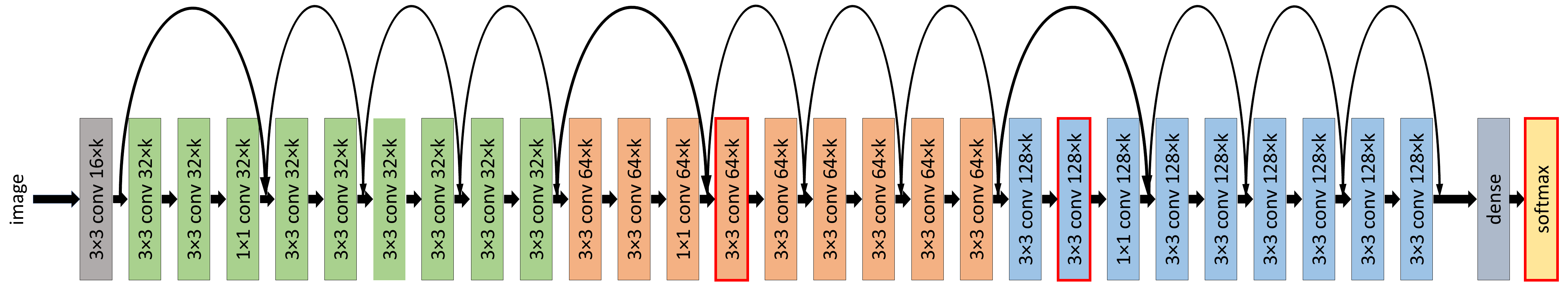
Figure 2: To investigate the impact of Nullspace Tuning on the feature space, we visualize extracted feature maps for both MixMatch and MixMatchNST models. The convolutional operations in the Wide ResNet-28 model are bordered in red where we choose to extract the feature maps for all test images in CIFAR-10 for each chosen model.

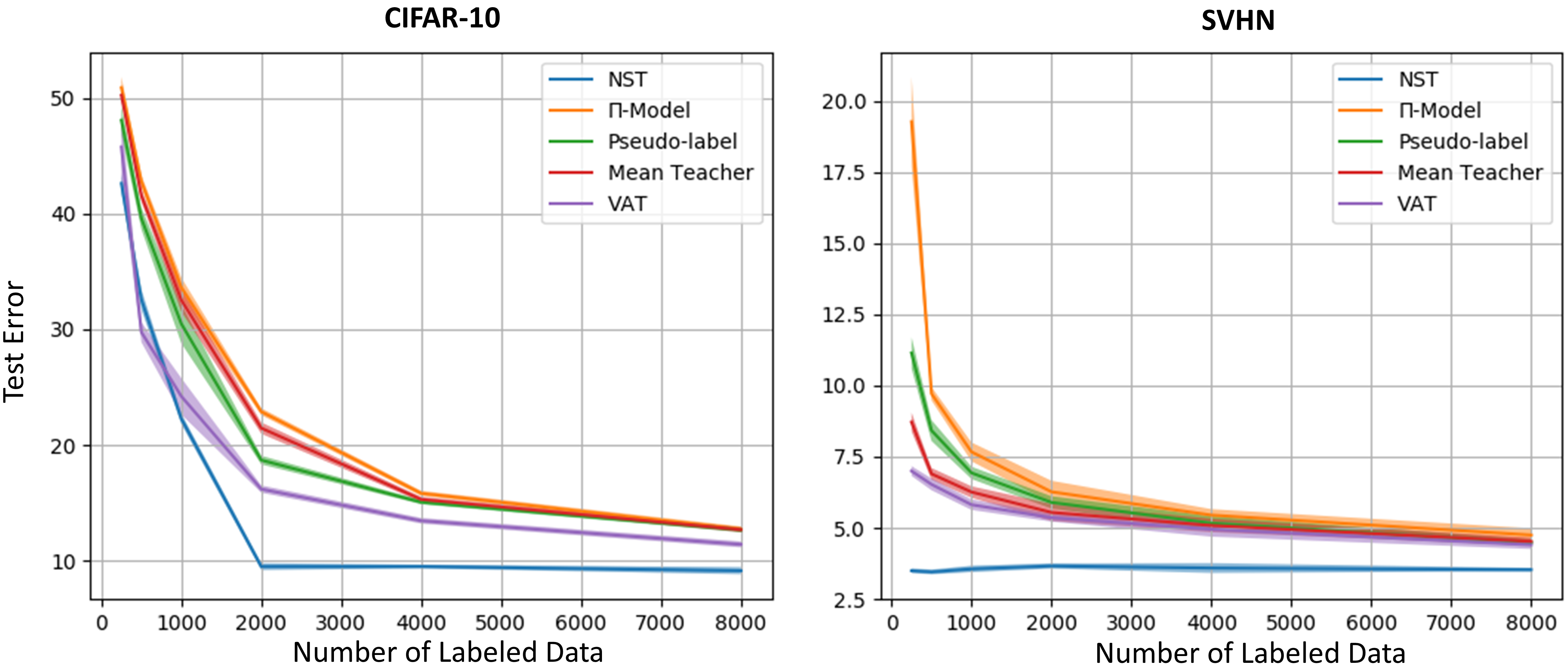
Figure 3: The added partial label information results in a substantial improvement in performance over baseline methods. This is shown in a percent test error and standard deviation (shaded region) comparison of Nullspace Tuning to baseline methods on CIFAR-10 (left) and SVHN (right) for a varied number of labeled data between 250 and 8000. The most significant improvement between Nullspace Tuning and the next best performing method (VAT) occurs in CIFAR-10 at 2000 labeled data.

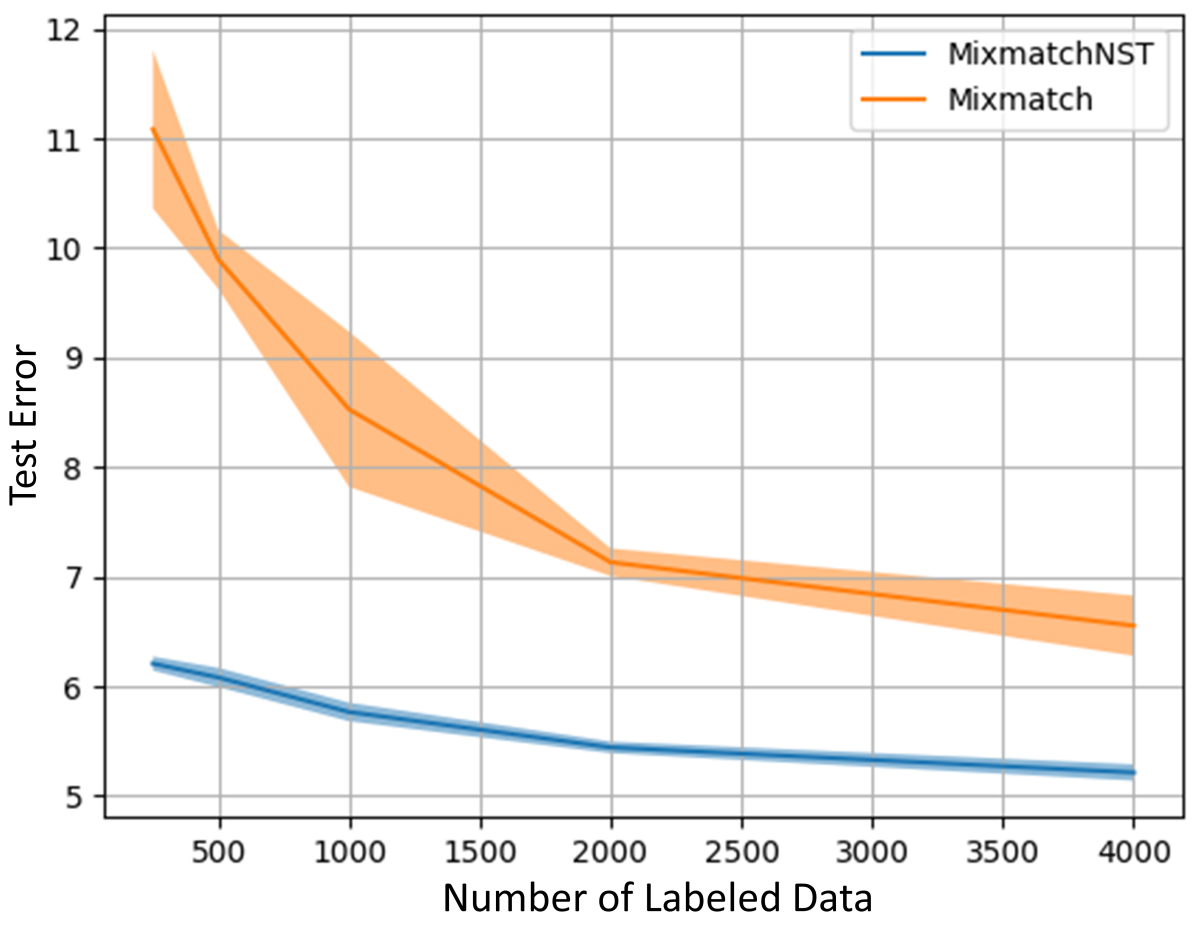
Figure 4: The additive performance of Nullspace Tuning on top of the state-of-the-art MixMatch algorithm is considerable. This is especially evident at 250 labeled data in CIFAR-10 where error is reduced by a factor of 1.8. This is shown in a percent test error and standard deviation (shaded regions) comparison of MixMatchNST to MixMatch on CIFAR-10 for a varying number of labels.

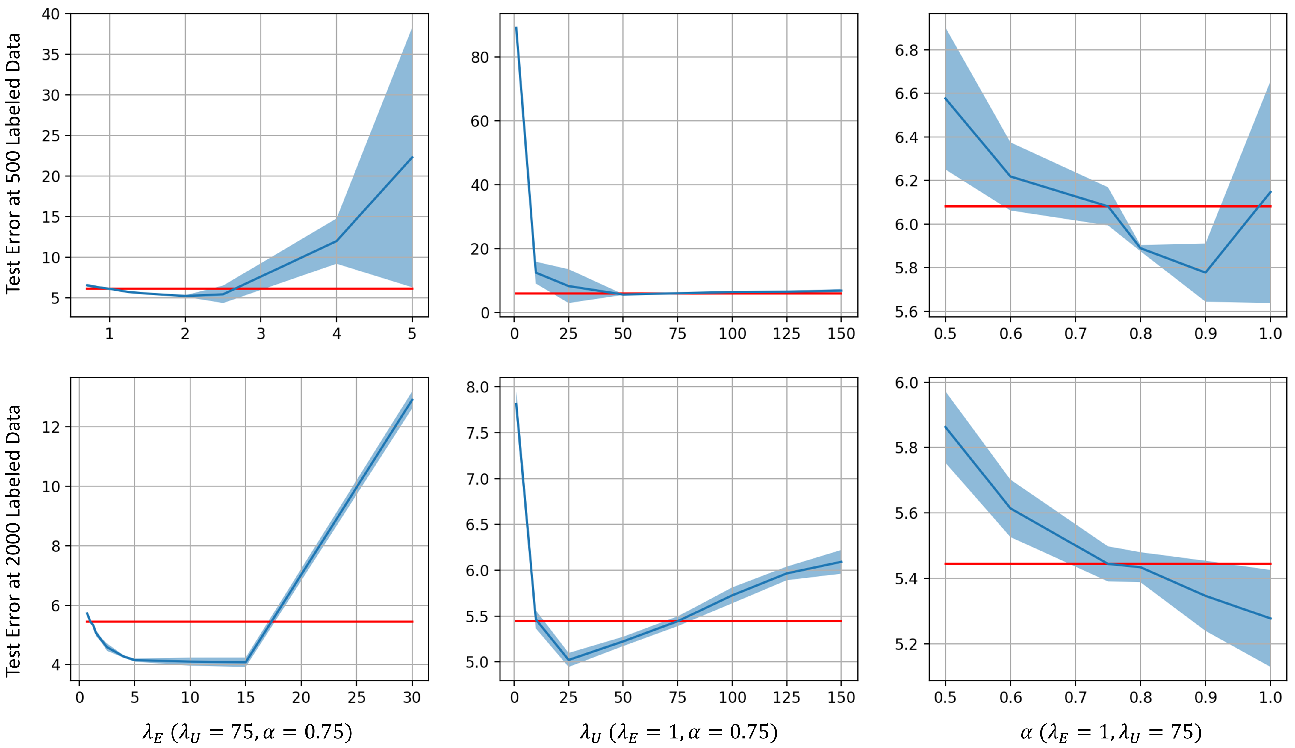
Figure 5: MixMatchNST models can benefit from hyperparameter tuning at each number of labeled data. The hyperparametr $\lambda_{E}$ shows the greatest need for this as the optimal value at 2000 labeled data is at least double of that at 500 labeled data and would reduce the test error by approximately 1.4%. Test errors and standard deviations are reported (shaded regions) at 500 labeled data (top) and 2000 labeled data (bottom) as the hyperparameter space is searched for $\lambda_{E}$ (left), $\lambda_{U}$ (center), and $\alpha$ (right). Red lines indicate the performance before fine tuning. As one hyperparameter is tuned, the other two are set to the previously used values. The error achieved with the hyperparameters in Figure 4 is indicated by the red line.

3 Methods

This section describes the method of Nullspace Tuning using partial labels. We describe it first as a standalone approach, and then to illustrate how it can be combined with existing methods, we describe it in combination with MixMatch.

3.1 Null Space Tuning

Given a set of labeled data $\{x_{i},y_{i}\}\in D$ and unlabeled data $\{x^{*}_{i}\}\in D^{*}$ for which some equivalence classes are known, we perform Nullspace Tuning by adding to a standard loss function $\mathcal{L}_{s}$ a penalty on the difference in the predicted probabilities for pairs of elements of $D^{*}$. So the new loss function $\mathcal{L}$ becomes

$$\mathcal{L}=\mathcal{L}_{s}(h(x_{i}),y_{i})+\lambda||h(x^{*}_{j})-h(x^{*}_{k})||_{2}^{2}$$ (3)

where $h$ is the vector-valued prediction function of the model, $\lambda$ is a hyperparameter weighting the contribution of the nullspace loss term, and $x^{*}_{j}\sim x^{*}_{k}$ is known. Note that $x^{*}_{j}$ and $x^{*}_{k}$ have no required relationship to the labeled $x_{i}$, and randomization of the choice in unlabeled pairs could be a source of further data augmentation. In our first experiment, we use cross entropy as the standard loss function component $\mathcal{L}_{s}$.

3.2 MixMatchNST

In our second experiment, we modify the MixMatch loss function with a Nullspace Tuning term, and denote this model MixMatchNST. In brief, MixMatch assigns a guessed label $q$ to each unlabeled example $x^{*}$ by averaging the model’s predicted class distributions across $K$ augmentations of $x^{*}$. Temperature sharpening is then applied to the probability distribution of guessed labels to lower the entropy of those predictions for each example(Goodfellow et al., 2016). Mixup (Zhang et al., 2017) is then applied to the labeled data $\{x_{i},y_{i}\}$ and unlabeled data $\{x^{*}_{j},q_{j}\}$ to produce interpolated data $\{\tilde{x}_{i},\tilde{y}_{i}\}$ and $\{\tilde{x}^{*}_{j},\tilde{q}_{j}\}$. Mixup is parameterized by $\alpha$, which controls how far the interpolated examples may fall from the original examples. Weight decay is used during training to prevent overfitting (Loshchilov & Hutter, 2018)(Zhang et al., 2018).

With the addition of Nullspace Tuning, the loss function for MixMatchNST becomes a combination of terms: the loss term $\mathcal{L}_{X}$ for labeled data, which in this case is the cross-entropy loss $\mathcal{L}_{s}$, the MixMatch loss term $\mathcal{L}_{U}$ for unlabeled data and guessed labels, and the Nullspace Tuning loss term $\mathcal{L}_{E}$:

$$\mathcal{L}_{X}=\mathcal{L}_{s}(h(\tilde{x}_{i}),\tilde{y}_{i})$$ (4)

$$\mathcal{L}_{U}=||h(\tilde{x}^{*}_{j})-\tilde{q}_{j})||_{2}^{2}$$ (5)

$$\mathcal{L}_{E}=||q_{j}-q_{k}||_{2}^{2}$$ (6)

$$\mathcal{L}=\mathcal{L}_{X}+\lambda_{U}\mathcal{L}_{U}+\lambda_{E}\mathcal{L}_{E}$$ (7)

where $\lambda_{U}$ and $\lambda_{E}$ are hyperparameters controlling the balance of terms, and $x^{*}_{k}$ is chosen so that $x^{*}_{j}\sim x^{*}_{k}$ . The added Nullspace Tuning term (6) is calculated between the guessed labels $q_{j}$ and $q_{k}$ before the MixUp step, whereas the MixMatch terms (4) and (5) are calculated using interpolated, post-MixUp examples, as usual.

4 Experiments

We evaluate the benefit of Nullspace Tuning over partial label information using standard benchmark datasets. We follow the precedent of simulating randomly unlabeled data in these datasets, and we likewise simulate partial labels and their equivalence classes.

4.1 Implementation details

All experiments use a ”Wide ResNet-28” model (Zagoruyko & Komodakis, 2016), with modifications made to the loss function as needed to instantiate the various comparison methods. The training procedure and error reporting follows Oliver (2018) in experiment 1, and Berthelot (2019) in experiment 2.

4.1.1 Experiment 1

In Experiment 1 the simple use of Nullspace Tuning over partial labels was compared against four good semi-supervised learning methods, using benchmark datasets CIFAR-10 (Krizhevsky & Hinton, 2009) and SVHN (Netzer et al., 2011), and the comparison framework designed by Oliver (2018) re-implemented in PyTorch (Paszke et al., 2017). The comparison methods were $\Pi$-Model (Laine & Aila, 2016)(Sajjadi et al., 2016), Mean Teacher (Tarvainen & Valpola, 2017), VAT (Miyato et al., 2018), and Pseudo-Label (Lee, 2013), all using the Oliver framework (Oliver et al., 2018).

To simulate semi-supervised data, labels were removed from the majority of training data, leaving a small portion of labeled data, the size of which was systematically varied as part of the experiment. To simulate partial label information, equivalence classes were computed on the set chosen to be unlabeled, but before the labels were removed, one equivalence class per unique label value. Performance in these experiments represents an upper bound on the benefit we can expect to achieve using Nullspace Tuning over similar data, because natural partial labels are not always known so completely.

Test error and standard deviation was computed for labeled dataset sizes between 250 and 8000, for five randomly seeded splits each. CIFAR-10 has a total of 50000 examples of which 5000 are set aside for validation, and SVHN a total of 73257 of which 7325 are set aside for validation. The standard test set for each dataset are used to evaluate models. Hyperparameters for this experiment were set to those used by Oliver (2018).

4.1.2 Experiment 2

In Experiment 2 we evaluate the benefit of adding Nullspace Tuning to an existing powerful semi-supervised learning approach. MixMatch is a good example for this demonstration, because aside from being state of the art, it uses several techniques in combination already, and therefore has a fairly complex loss function.

Unlabeled and partially labeled examples were computed as in Experiment 1. For this experiment, we evaluate only on CIFAR-10, on which MixMatch has previously achieved the largest error reduction compared to other methods (Berthelot et al., 2019). We used the TensorFlow (Abadi et al., 2016) MixMatch implementation, written by the original authors (Berthelot et al., 2019), augmenting it to produce our MixMatchNST algorithm. Test error and standard deviation was computed for labeled dataset sizes between 250 and 4000, with five random splits each.

MixMatch hyperparameters were set at the optimal CIFAR-10 settings established by Berthelot. For MixMatchNST we set the Nullspace Tuning weight $\lambda_{E}=1$, which generally works well for most experiments. However, to investigate whether the addition of the Nullspace Tuning term altered the loss landscape, we also performed univariate grid search over the MixUp hyperparameter $\alpha$ and the loss component weights $\lambda_{E}$ and $\lambda_{U}$ for MixMatchNST. We did not apply a linear rampup (Tarvainen & Valpola, 2017) to $\lambda_{E}$ as is done for $\lambda_{U}$.

To investigate how the network was responding to Nullspace Tuning, we visualized three layers in the Wide ResNet-28 model (Figure 2) for both MixMatch and MixMatchNST. The feature maps for the CIFAR-10 test set were extracted after training with 500 and 2000 labeled examples and then were reshaped in to a vector for each sample. These flattened feature maps were then embedded in a 2D manifold fit with UMAP (McInnes et al., 2018) resulting in a single coordinate for each sample.

Table 1: CIFAR-10 and SVHN percent classification error is reported here for all methods at 250 and 2000 labeled data. Bolded values indicate the best performing method for the number of labeled data in the dataset.

method	cifar-10 error	cifar-10 error	svhn error	svhn error
	250 labeled data	2000 labeled data	250 labeled data	2000 labeled data
$\Pi$-Model	50.88$\pm$ 0.94	22.88$\pm$ 0.30	19.28$\pm$ 1.58	6.27$\pm$ 0.39
Mean Teacher	50.22$\pm$ 0.0.39	21.46$\pm$ 0.49	8.72$\pm$ 0.33	5.54$\pm$ 0.30
Pseudo-label	48.06$\pm$ 1.24	18.70$\pm$ 0.38	11.15$\pm$ 0.55	5.89$\pm$ 0.22
VAT	45.76$\pm$ 2.81	16.19$\pm$ 0.32	7.00$\pm$ 0.17	5.36$\pm$ 0.14
NST	42.60$\pm$ 0.82	9.50$\pm$ 0.30	3.49$\pm$ 0.08	3.66$\pm$ 0.10
MixMatch	11.08$\pm$ 0.72	7.13$\pm$ 0.13	NA	NA
MixMatchNST	6.21$\pm$ 0.06	5.44$\pm$ 0.05	NA	NA

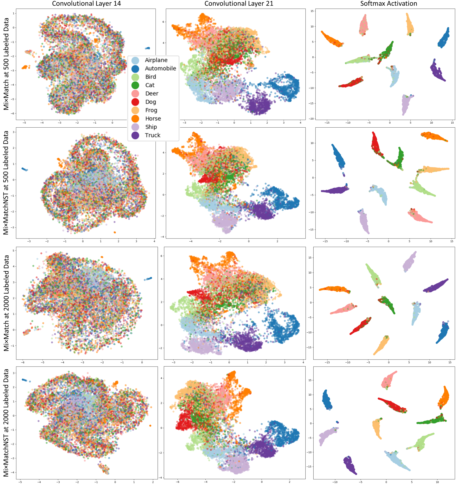
Figure 6: Nullspace Tuning provides better learning with fewer labeled examples, as evidenced by discernably clearer clusters in a 2D manifold space learned from the feature maps. In general, MixMatchNST does about as well in the CIFAR-10 test set with 500 labeled training points (second row) as MixMatch does with 2000 (third row). Each point represents a sample’s feature maps flattened to a single vector from two convolutional layers (first and second column) and the final softmax layer (third column), embedded in a 2D space learned with UMAP (McInnes et al., 2018). These are shown for a single fold for MixMatch and MixMatchNST for datasets with 500 (top two rows) and 2000 (bottom two rows) labeled examples. With 500 labeled examples, a cluster is forming at layer 14 for the class ”Airplane” in MixMatchNST, with no clear counterpart in MixMatch. At layer 21, several clusters are slightly clearer, with separation between Cat and Dog further along. With 2000 labeled examples, both methods are starting to form clusters for Airplane at layer 14, but MixMatchNST now also has a cluster formed for ”Ship”. At layer 21, several clusters are again slightly clearer for MixMatchNST, with separation especially evident for ”Frog”.

4.2 Results

4.2.1 Experiment 1

The use of partial labels generally provided a performance improvement at least as large as the difference between the best and the worst semi-supervised methods, except at the smallest labeled set sizes (Figure 3). Surprisingly, the benefit of partial labels essentially maxes out at the relatively small number of 2000 labeled examples (vs. 43000 unlabeled examples) in CIFAR-10, and at less than 250 examples (vs. 65682 unlabeled examples) in SVHN, while the semi-supervised methods continue to improve with more labeled data.

4.2.2 Experiment 2

The performance of MixMatch on CIFAR-10 was far better than any algorithm, including Nullspace Tuning, in Experiment 1 (Figure 3). Despite this impressive gain, performance was improved further by including Nullspace Tuning together with the MixMatch innovations. Doing so reduced test error by an additional factor of 1.8 on the smallest labeled set size, and about 1.3 at the largest set size (Figure 4).

The hyperparameter search shows that the MixMatch loss landscape was modestly altered with respect to the MixMatch hyperparameters $\alpha$ and $\lambda_{U}$, and small gains could be had by tuning them further (Figure 5). Tuning our nullspace weight made a larger relative difference, providing a further improvement of about 20% at 500 labeled datapoints, and about 30% at 2000 labeled datapoints, over what is shown in Figure 4.

Image features from MixMatch models and MixMatchNST models show that comparable learning happens with fewer examples with the addition of Nullspace Tuning (Figure 6), and that this learning occurs deep inside the model, rather than superficially at a later layer. The clusters in convolutional layers under Nullspace Tuning with 500 labeled examples look comparable to those for 2000 labeled examples without it, and the clustering appears slightly clearer with Nullspace Tuning given the same number of labeled examples. Differences in the softmax layer are subtler, but their presence is evident by the overall model performance.

5 Discussion

The main contribution of this work is the systematic demonstration that tuning the nullspace of a model using the partial label information that may reside in unlabeled data can provide a substantial performance boost compared to treating them as purely unlabeled data. It is not surprising that adding new information to a model provides such an improvement; our goal with this work was to quantify just how much improvement one could expect if equivalence classes were known within the unlabeled data.

This idea is important because identifying or obtaining equivalence classes within unlabeled data may be cheaper than obtaining more labels, if standard semi-supervised methods provide insufficient performance.

The gain from using partial label information is fairly constant over the range of labeled dataset size tested, as long as a minimum threshold of labeled data is met. This makes sense from the perspective of tuning the null space of the model, because most of that tuning can be done with equivalence classes, but a small amount of labeled data is needed to anchor what is learned to the correct labels.

Increasing the number of labeled examples beyond the threshold is essentially trading partial label information for full label information. The relative value of that information for a given learning problem is suggested by the slope of the error curve. For experiment 1, the nearly horizontal slope suggests that partial information is nearly as good as full label information. The performance of the architecture on a fully-labeled dataset was $2.59\%$ error, which reinforces this idea. The steeper (but still mild) slope found in Experiment 2 suggests a stronger tradeoff, although performance of MixMatch on the full $50,000$ examples is $4.2\%$ (Berthelot et al., 2019), which is fairly close to the $5.5\%$ that we get using more than $90\%$ partial labels, or even the $6.0\%$ that we get with $99\%$ partial labels. We conclude that at least in some cases, partial labels can get us most of the way there.

We can infer something about what the models are learning from the ordering of model performance: MixMatchNST $>$ MixMatch $>$ Nullspace Tuning $>$ single data-augmentation models. Explicitly learning the shape of the nullspace from partial labels was much more effective than implicitly placing data transformations into that space by the algorithms in Experiment 1, although combining those transformations into MixMatch was more effective still. But the fact that MixMatchNST performed better than either MixMatch or Nullspace Tuning alone demonstrates that MixMatch is learning somewhat different aspects of the nullspace than that provided by the partial labels.

One strength of this method is its simplicity — it can be added to nearly any other semi-supervised learning algorithm, as long as we have access to the loss function, and we can provide appropriate example pairs from an equivalence class.

This experiment used the largest possible equivalence classes — one class for each label value. Naturally occurring equivalence classes are likely not to be so large, especially if they are obtained by repeated observations of the same object. Our experimental design investigated the most we could gain from using the partial information in equivalence classes, but if the classes are smaller and more numerous, then we might expect that gain to be smaller. But because the partial labels are given to the algorithm as example pairs, with no required relationship between those pairs and the labeled pairs, Nullspace Tuning can still be used even with equivalence classes as small as two examples. And if those equivalence classes are well distributed over the data space, their diminished size may not actually impact the benefit by much. One could imagine that even a relatively small number of relatively small equivalence classes could be rather effective at tuning the null space. The large number of trained models needed to characterize how the benefit changes with respect to the size and number of equivalence classes placed that question out of scope for this paper, but it will be an interesting direction for future work.

And of course, not all learning problems have natural equivalence classes embedded in them at all. Benchmark public datasets tend not to, except in simulations like ours, partly because information about how they were collected has been lost. But it may be cheap to instrument data collection pipelines to record information that does provide this information. In addition to the medical use cases described above, where the patient identity is tracked through repeated observations, unlabeled objects may be tracked through sequential video frames, fixed but unlabeled regions may be identified for multiple passes of a satellite, or the unlabeled sentiment of all sentences in a paragraph might be considered to form an equivalence class. We expect that there are many creative ways to find partial labels in naturally occurring datasets, and when we find them, Nullspace Tuning is a promising method to exploit them.

Nullspace turning is a flexible approach that is amenable to real world learning scenarios and promises to enable use of partial label information that is not accessible with current standard neural network approaches.

5.1 Acknowledgments

This work was supported by the National Institutes of Health under award numbers R01EB017230, and T32EB001628, and in part by the National Center for Research Resources, Grant UL1 RR024975-01. The content is solely the responsibility of the authors and does not necessarily represent the official views of the NIH. This study was in part using the resources of the Advanced Computing Center for Research and Education (ACCRE) at Vanderbilt University, Nashville, TN which is supported by NIH S10 RR031634.

References

- Abadi et al. (2016) Abadi, M., Barham, P., Chen, J., Chen, Z., Davis, A., Dean, J., Devin, M., Ghemawat, S., Irving, G., Isard, M., et al. Tensorflow: A system for large-scale machine learning. In 12th USENIX Symposium on Operating Systems Design and Implementation (OSDI 16), pp. 265–283, 2016.
- Berthelot et al. (2019) Berthelot, D., Carlini, N., Goodfellow, I., Papernot, N., Oliver, A., and Raffel, C. A. Mixmatch: A holistic approach to semi-supervised learning. In Advances in Neural Information Processing Systems, pp. 5050–5060, 2019.
- Bromley et al. (1994) Bromley, J., Guyon, I., LeCun, Y., Säckinger, E., and Shah, R. Signature verification using a” siamese” time delay neural network. In Advances in neural information processing systems, pp. 737–744, 1994.
- Chapelle et al. (2006) Chapelle, O., Schölkopf, B., and Zien, A. Semi-supervised learning. MIT Press, 2006.
- Chung et al. (2017) Chung, D., Tahboub, K., and Delp, E. J. A two stream siamese convolutional neural network for person re-identification. In Proceedings of the IEEE International Conference on Computer Vision, pp. 1983–1991, 2017.
- Ciregan et al. (2012) Ciregan, D., Meier, U., and Schmidhuber, J. Multi-column deep neural networks for image classification. In 2012 IEEE conference on computer vision and pattern recognition, pp. 3642–3649. IEEE, 2012.
- Cireşan et al. (2010) Cireşan, D. C., Meier, U., Gambardella, L. M., and Schmidhuber, J. Deep, big, simple neural nets for handwritten digit recognition. Neural computation, 22(12):3207–3220, 2010.
- Cubuk et al. (2019) Cubuk, E. D., Zoph, B., Mane, D., Vasudevan, V., and Le, Q. V. Autoaugment: Learning augmentation strategies from data. In Proceedings of the IEEE conference on computer vision and pattern recognition, pp. 113–123, 2019.
- Dirix et al. (2009) Dirix, P., Vandecaveye, V., De Keyzer, F., Stroobants, S., Hermans, R., and Nuyts, S. Dose painting in radiotherapy for head and neck squamous cell carcinoma: value of repeated functional imaging with 18f-fdg pet, 18f-fluoromisonidazole pet, diffusion-weighted mri, and dynamic contrast-enhanced mri. Journal of Nuclear Medicine, 50(7):1020–1027, 2009.
- Freeborough & Fox (1997) Freeborough, P. A. and Fox, N. C. The boundary shift integral: an accurate and robust measure of cerebral volume changes from registered repeat mri. IEEE transactions on medical imaging, 16(5):623–629, 1997.
- Goodfellow et al. (2016) Goodfellow, I., Bengio, Y., and Courville, A. Deep learning. MIT press, 2016.
- Huo et al. (2019) Huo, Y., Terry, J. G., Wang, J., Nath, V., Bermudez, C., Bao, S., Parvathaneni, P., Carr, J. J., and Landman, B. A. Coronary calcium detection using 3d attention identical dual deep network based on weakly supervised learning. In Medical Imaging 2019: Image Processing, volume 10949, pp. 1094917. International Society for Optics and Photonics, 2019.
- Krizhevsky & Hinton (2009) Krizhevsky, A. and Hinton, G. Learning multiple layers of features from tiny images. Technical report, Citeseer, 2009.
- Krizhevsky et al. (2012) Krizhevsky, A., Sutskever, I., and Hinton, G. E. Imagenet classification with deep convolutional neural networks. In Advances in neural information processing systems, pp. 1097–1105, 2012.
- Kumar et al. (2016) Kumar, B., Carneiro, G., Reid, I., et al. Learning local image descriptors with deep siamese and triplet convolutional networks by minimising global loss functions. In Proceedings of the IEEE Conference on Computer Vision and Pattern Recognition, pp. 5385–5394, 2016.
- Laine & Aila (2016) Laine, S. and Aila, T. Temporal ensembling for semi-supervised learning. arXiv preprint arXiv:1610.02242, 2016.
- Lee (2013) Lee, D.-H. Pseudo-label: The simple and efficient semi-supervised learning method for deep neural networks. In Workshop on Challenges in Representation Learning, ICML, volume 3, pp. 2, 2013.
- Loshchilov & Hutter (2018) Loshchilov, I. and Hutter, F. Fixing weight decay regularization in adam. 2018.
- McInnes et al. (2018) McInnes, L., Healy, J., and Melville, J. Umap: Uniform manifold approximation and projection for dimension reduction. arXiv preprint arXiv:1802.03426, 2018.
- McLaughlin et al. (2016) McLaughlin, N., Martinez del Rincon, J., and Miller, P. Recurrent convolutional network for video-based person re-identification. In Proceedings of the IEEE conference on computer vision and pattern recognition, pp. 1325–1334, 2016.
- Miyato et al. (2018) Miyato, T., Maeda, S.-i., Koyama, M., and Ishii, S. Virtual adversarial training: a regularization method for supervised and semi-supervised learning. IEEE transactions on pattern analysis and machine intelligence, 41(8):1979–1993, 2018.
- Nath et al. (2018) Nath, V., Parvathaneni, P., Hansen, C. B., Hainline, A. E., Bermudez, C., Remedios, S., Blaber, J. A., Schilling, K. G., Lyu, I., Janve, V., et al. Inter-scanner harmonization of high angular resolution dw-mri using null space deep learning. In International Conference on Medical Image Computing and Computer-Assisted Intervention, pp. 193–201. Springer, 2018.
- Netzer et al. (2011) Netzer, Y., Wang, T., Coates, A., Bissacco, A., Wu, B., and Ng, A. Y. Reading digits in natural images with unsupervised feature learning. 2011.
- Oliver et al. (2018) Oliver, A., Odena, A., Raffel, C. A., Cubuk, E. D., and Goodfellow, I. Realistic evaluation of deep semi-supervised learning algorithms. In Advances in Neural Information Processing Systems, pp. 3235–3246, 2018.
- Paszke et al. (2017) Paszke, A., Gross, S., Chintala, S., Chanan, G., Yang, E., DeVito, Z., Lin, Z., Desmaison, A., Antiga, L., and Lerer, A. Automatic differentiation in pytorch. 2017.
- Perez & Wang (2017) Perez, L. and Wang, J. The effectiveness of data augmentation in image classification using deep learning. arXiv preprint arXiv:1712.04621, 2017.
- Sajjadi et al. (2016) Sajjadi, M., Javanmardi, M., and Tasdizen, T. Regularization with stochastic transformations and perturbations for deep semi-supervised learning. In Advances in Neural Information Processing Systems, pp. 1163–1171, 2016.
- Sato et al. (2015) Sato, I., Nishimura, H., and Yokoi, K. Apac: Augmented pattern classification with neural networks. arXiv preprint arXiv:1505.03229, 2015.
- Schroff et al. (2015) Schroff, F., Kalenichenko, D., and Philbin, J. Facenet: A unified embedding for face recognition and clustering. In Proceedings of the IEEE conference on computer vision and pattern recognition, pp. 815–823, 2015.
- Simard et al. (2003) Simard, P. Y., Steinkraus, D., Platt, J. C., et al. Best practices for convolutional neural networks applied to visual document analysis. In Icdar, volume 3, 2003.
- Tarvainen & Valpola (2017) Tarvainen, A. and Valpola, H. Mean teachers are better role models: Weight-averaged consistency targets improve semi-supervised deep learning results. In Advances in neural information processing systems, pp. 1195–1204, 2017.
- Varior et al. (2016) Varior, R. R., Haloi, M., and Wang, G. Gated siamese convolutional neural network architecture for human re-identification. In European conference on computer vision, pp. 791–808. Springer, 2016.
- Verma et al. (2019) Verma, V., Lamb, A., Kannala, J., Bengio, Y., and Lopez-Paz, D. Interpolation consistency training for semi-supervised learning. arXiv preprint arXiv:1903.03825, 2019.
- Wan et al. (2013) Wan, L., Zeiler, M., Zhang, S., Le Cun, Y., and Fergus, R. Regularization of neural networks using dropconnect. In International conference on machine learning, pp. 1058–1066, 2013.
- Yankelevitz et al. (1999) Yankelevitz, D. F., Gupta, R., Zhao, B., and Henschke, C. I. Small pulmonary nodules: evaluation with repeat ct—preliminary experience. Radiology, 212(2):561–566, 1999.
- Zagoruyko & Komodakis (2016) Zagoruyko, S. and Komodakis, N. Paying more attention to attention: Improving the performance of convolutional neural networks via attention transfer. arXiv preprint arXiv:1612.03928, 2016.
- Zhang et al. (2018) Zhang, G., Wang, C., Xu, B., and Grosse, R. Three mechanisms of weight decay regularization. arXiv preprint arXiv:1810.12281, 2018.
- Zhang et al. (2017) Zhang, H., Cisse, M., Dauphin, Y. N., and Lopez-Paz, D. mixup: Beyond empirical risk minimization. arXiv preprint arXiv:1710.09412, 2017.
- Zhu & Goldberg (2009) Zhu, X. and Goldberg, A. B. Introduction to semi-supervised learning. Synthesis lectures on artificial intelligence and machine learning, 3(1):1–130, 2009.
- Zhu et al. (2003) Zhu, X., Ghahramani, Z., and Lafferty, J. D. Semi-supervised learning using gaussian fields and harmonic functions. In Proceedings of the 20th International conference on Machine learning (ICML-03), pp. 912–919, 2003.
- Zhu (2005) Zhu, X. J. Semi-supervised learning literature survey. Technical report, University of Wisconsin-Madison Department of Computer Sciences, 2005.