Diagnosing the R$\acute{e}$nyi Holographic Dark Energy model in a flat Universe

Abstract

Abstract

In this paper, we have examined the R$\acute{e}$nyi holographic dark energy (RHDE) model in the framework of an isotropic and spatially homogeneous flat FLRW (Friedmann- Lema$\hat{i}$tre-Robertson-Walker) Universe by considering different values of parameter $\delta$, where the infrared cut-off is taken care by the Hubble horizon. We examined the RHDE model through the analysis of the growth rate of perturbations and the statefinder hierarchy. The evolutionary trajectories of the statefinder hierarchy $S_{3}^{1}$, $S_{3}^{2}$ $S_{4}^{1}$, $S_{4}^{2}$ versus redshift $z$, shows satisfactory behaviour throughout the Universe evolution. One of the favourable appliance for exploring the dark energy models is the CND (composite null diagnostic) $\{S_{3}^{1}-\epsilon\}$ and $\{S_{4}^{1}-\epsilon\}$, where the evolutionary trajectories of the $\{S_{3}^{1}-\epsilon\}$ and $\{S_{4}^{1}-\epsilon\}$ pair show remarkable characteristics and the departure from $\Lambda$CDM could be very much assessed.

Keywords: RHDE; statefinder hierarchy; composite null diagnostic(CND).
PACS: 98.80.Es, 95.36.+x, 98.80.Ck

I Introduction

Presently cosmologists are facing the problem to understand the reason behind the cosmic acceleration ref1 ; ref2 . This can be explained by one of the methods known as the concept of dark energy (DE). But the nature of DE is not known yet. Various experiments like LSST ref3 , DES ref4 , WFIRST ref5 and DESI ref6 will survey the Universe to understand the nature of DE. Adjoint to these surveys, the accelerated expansion of the universe are supported by various observations like CMBR anisotropies, BAO, SNeIa and LSS formation and WL, which is also consistent with the current standard cosmological model $\Lambda$CDM, where $\Lambda$ is a constant component of cosmological fluid with the equation of state EoS $\omega=-1$. Evolution of the cosmological constant is characterized as DE. Since we can only notice the impact of DE on the Hubble flow measuring observable components like radiation and matter. Therefore, we can not evaluate DE directly. Since the DE and gravity are associated in the standard model, we can compute the distribution of matter in the universe by $\omega=p(\rho)$, where $(\rho)$ is the matter-energy density and $p$ is the pressure. For simplicity, we take $\omega=p/\rho$.

Currently, discussion is around on the authenticity of $\Lambda$CDM model, which resulting disagreement between Plank ref7 and other cosmological measurements like strong lensing time delays (H0LiCOW), megamasers, Cefeids (SH0ES), tip of the red giant branch (TRGB) and Oxygenrich Miras and surface brightness fluctuations ref8 . These disagreements encourages one to examine other options to the concordance model. To imitate $\Lambda$ according to the cosmological observations at the present time, dynamical dark energy models are most interesting approach. Various approaches are extended theories of gravity ref9 , Bayesian reconstruction of a time-dependent EoS ref10 , dark energy parametrisations ref11 ; ref12 ; ref13 ; ref14 ; ref15 , $\omega(z)$ reconstructions ref16 , modify gravity ref17 ; ref18 , non-parametric reconstructions of $\omega(z)$ ref19 ; ref20 , quintessence scenarios ref21 ; ref22 and dynamical $\omega_{x}$ from $f(R)$ models ref23 ; ref24 . These models helps us in understanding the effects of DE. To describe the accelerated expansion of the cosmos motivated by holograpic principle ref25 ; ref26 ; ref27 ; ref28 , M. Li suggested Holographic dark energy (HDE) where IR cutoff was taken care by future event horizon ref29 . After that Agegrapic dark enrgy (ADE) model was suggested by Cai by taking length measure as the age of the Universe ref30 . By considering conformal time as time scale, Wei and Cai suggested the New agegraphic dark energy (NADE) model ref31 . Gao et al. ref32 suggested the Ricci dark energy model by replacing future event horizon with ricci scalar curvature. For investigation of the cosmological and gravitational and incidences recently, different entropies ref33 ; ref34 ; ref35 ; ref36 has been used to find new form of DE models such as Tsallis holographic dark energy (THDE) model ref37 , Tsallis agegraphic dark energy (TADE) model ref38 , R$\acute{e}$nyi holograpic dark energy (RHDE) model ref39 and and Sharma-Mittal holograpic dark energy (SMHDE) model ref40 . Researchers had used these newly proposed dark energy models in different scenariosref41 ; ref42 ; ref43 ; ref44 ; ref45 ; ref46 ; ref47 ; ref48 ; ref49 ; ref50 ; ref51 ; ref52 ; ref53 .

Therefore, there is an absolute need for the diagnostic tools which can discriminate these various form of dark energy models. Keeping this in mind, different diagnostic tools are proposed to discriminate among various DE models. In ref54 , authors proposed the growth rate of linear perturbations and statefinder hierarchy, as null diagnostics to differentiate among different dark energy models from $\Lambda$CDM model. The statefinder hierarchy is a geometrical diagnostic which involves higher-order differential coefficients of scale factor $a(t)$, and also model-independent ref55 . Statefinder hierarchy has been used to discrimination among BMG (Bimetric Massive Gravity) theory, DGP models and MGG (Modified Galileon Gravity) ref56 . To differentiate the HDE models and breaking the degeneracy, the statefinder hierarchy has been investigated in ref57 . To discriminate among purely kinetic $k$-essence, modified Chaplygin gas, superfluid Chaplygin gas, generalized Chaplygin gas and $\Lambda$CDM model and for analysing the deviation from the $\Lambda$CDM model, the statefinder hierarchy and growth rate of perturbation has been used ref58 ; ref59 . The statefinder hierarchy and the growth rate of perturbations are used in ref60 ; ref61 ; ref62 ; ref63 ; ref64 ; ref65 ; ref66 ; ref67 ; ref68 ; ref69 ; ref70 ; ref71 ; ref72 . Using statefinder hierarchy in the non-flat Universe considering IR cutoff as apparent horizon has been investigated by one of the authors of present work for the THDE models ref73 .

In this work, we have explored the newly proposed R$\acute{e}$nyi Holographic Dark Energy (RHDE) model through the diagnostic tools described above in the flat FRW Universe by taking the Hubble horizon as an infrared cutoff, which has not been explored earlier. Also, we have examined the deviation of the RHDE model from $\Lambda$CDM using these diagnostic tools. The paper is structured as follows; In Sect. II, we in brief visit the R$\acute{e}$nyi holographic dark energy. Sect. III is dedicated to discussing the flat FRW cosmological model. Section IV is divided into two subsections A and B, for the methods of the statefinder hierarchy diagnostic and growth rate of perturbations analysis. Finally, in the last section, we have given inferences.

II R$\acute{E}$nyi Holographic Dark Energy Model

The form of the Bekenstein entropy of a system is $S=\frac{A}{4}$ , where $A=4\pi L^{2}$ and L is the IR cut-off. Another modified form of the R$\acute{e}$nyi entropy ref75 is given as:

$$S=\frac{1}{\delta}\log\left(\frac{\delta}{4}A+1\right)=S=\frac{1}{\delta}\log\left(\pi\delta L^{2}+1\right),$$ (1)

R$\acute{e}$nyi HDE density, by considering the assumption $\rho_{d}\ dV\ \propto\ TdS$, takes the following form:

$$\rho_{D}=\frac{3c^{2}}{8\pi L^{2}}(\pi\delta L^{2}+1)^{-1},$$ (2)

By taking Hubble horizon as an IR cut-off $L=\dfrac{1}{H}$, we obtained:

$$\rho_{D}=\frac{3c^{2}H^{2}}{8\pi\left(\frac{\pi\delta}{H^{2}}+1\right)},$$ (3)

where $c^{2}$ is a numerical constant as usual.

III The cosmological model

For the flat FRW Universe, the metric is given as :

$$ds^{2}=-dt^{2}+a^{2}(t)\Big{(}dr^{2}+r^{2}d\Omega^{2}\Big{)}.$$ (4)

In a flat FRW Universe, the Friedmann first equation, involving DM and RHDE is defined as :

$$H^{2}=\frac{1}{3}(8\pi G)\left(\rho_{D}+\rho_{m}\right),$$ (5)

where $\rho_{D}$ and $\rho_{m}$ represent the energy density of RHDE and matter, respectively. The energy density parameter of RHDE and pressureless matter with the help of the fractional energy densities, can be defined as

$$\Omega_{m}=\frac{8\pi\rho_{m}G}{3H^{2}},\hskip 28.45274pt\Omega_{D}=\frac{8\pi\rho_{D}G}{3H^{2}},$$ (6)

Now Eq. (5) with help of Eq. (6) can be written as:

$$1=\Omega_{D}+\Omega_{m}$$ (7)

The conservation law for matter and RHDE are given as :

$$\dot{\rho}_{m}+3H\rho_{m}=0,$$ (8)

$$\dot{\rho}_{D}+3H(\rho_{D}+p_{D})=0.$$ (9)

in which $\omega_{D}=p_{D}/\rho_{D}$ represents the RHDE EoS parameter. Now, using differential with time of Eq. (5) in Eq. (8), and Eq. (9) combined the result with the Eq. (7), we get

$$\frac{\dot{H}}{H^{2}}=\frac{3}{2}\left(\frac{\pi\delta\Omega_{D}}{\pi\delta\left(2\Omega_{D}-1\right)+\left(\Omega_{D}-1\right)H(t)^{2}}-1\right)$$ (10)

By Eq. (10), the deceleration parameter (DP) $q$ is found as

$q=-1-\frac{\dot{H}}{H^{2}}$

$$q=\frac{(1-2\delta)\Omega_{D}(t)+1}{2\left(1-(2-\delta)\Omega_{D}(t)\right)}$$ (11)

Also, by taking the derivative with respect to time of Eq. (3), we get

$$\dot{\rho_{D}}=2\rho_{D}\frac{\dot{H}}{H}\left(\frac{\pi\delta}{\pi\delta+H^{2}}+1\right)$$ (12)

Now by using the Eqs. (12) with Eqs. (9) and (10), we gets expression for EoS parameter as:

$$\omega_{D}=-\frac{\pi\delta}{\pi\delta\left(2\Omega_{D}-1\right)+H^{2}\left(\Omega_{D}-1\right)}.$$ (13)

Also, taking the time differential of the energy density parameter $\Omega_{D}$ with Eqs. (10) and (12), we find

$$\Omega_{D}^{\prime}=-\frac{3\pi c^{2}\delta H^{2}\left(\Omega_{D}-1\right)}{\left(\pi\delta+H^{2}\right)\left(\pi\delta\left(2\Omega_{D}-1\right)+H^{2}\left(\Omega_{D}-1\right)\right)}$$ (14)

where the dot is the derivative while considering time and prime lets us obtain the derivative concerning ln a.

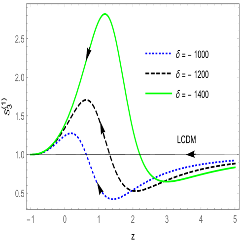
Figure 1: Graph of $S_{3}^{(1)}$ versus redshift z, for non- interacting RHDE with Hbbble radius as the IR cutoff. Here, $H(z=0)=70$, $\Omega_{D}(z=0)=0.73$ and different values of $\delta$.

IV The methods of diagnostic

In this work, we used two diagnostic tools, statefinder hierarchy and growth rate of perturbations. We shall explore the RHDE model to discriminate from $\Lambda$CDM model with the help of these two diagnostic tools in this section.

IV.1 The Statefinder Hierarchy diagnostic

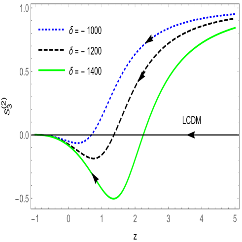
Figure 2: Graph of $S_{3}^{(2)}$ versus redshift z, for non- interacting RHDE with Hbbble radius as the IR cutoff. Here, $H(z=0)=70$, $\Omega_{D}(z=0)=0.73$ and different values of $\delta$.

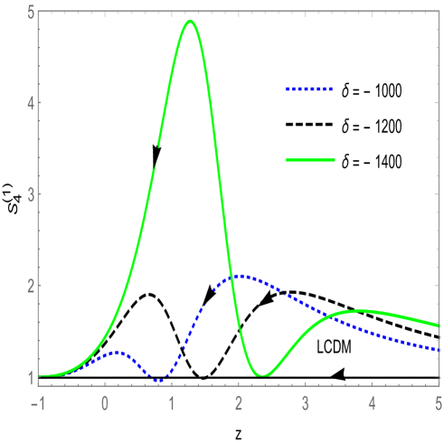
Figure 3: Graph of $S_{4}^{(1)}$ versus redshift z, for non- interacting RHDE with Hbbble radius as the IR cutoff. Here, $H(z=0)=70$, $\Omega_{D}(z=0)=0.73$ and different values of $\delta$.

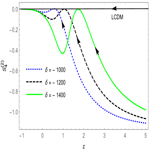
Figure 4: Graph of $S_{4}^{(2)}$ versus redshift z, for non- interacting RHDE with Hbbble radius as the IR cutoff. Here, $H(z=0)=70$, $\Omega_{D}(z=0)=0.73$ and different values of $\delta$.

Here, statefinder hierarchy diagnostic will be reviewed for the RHDE model will be described. The Taylor expansion of the scale factor $\frac{a(t)}{a_{0}}=\frac{1}{z+1}$, around the present epoch ${t_{0}}$ is given as:

$$\frac{a(t)}{a_{0}}=\sum_{n=1}^{\infty}\frac{A_{n}(t_{0})}{n!}\left[H_{0}\left(t-t_{0}\right)\right]{}^{n}$$ (15)

Where $A_{n}=\frac{a^{n}}{aH^{n}}$, ${a^{n}}$ is the $n^{th}$ derivative of the scale factor a verses cosmic time t and n $\in$ N. The statefinder hierarchy $S_{n}$ is defined as follows ref75a :

$$S_{2}=A_{2}+\frac{3\Omega_{m}}{2},S_{3}=A_{3}\quad and\quad S_{4}=A_{4}+\frac{9\Omega_{m}}{2},$$ (16)

Aforementioned gives the diagnostics for the model ($\Lambda$CDM) with $n\geq 3$, i.e., $S_{n}|\Lambda$CDM = 1. Hence by the use of $\Omega_{m}=\frac{2(q+1)}{3}$ the statefinder hierarchy $S_{3}^{(1)}$, $S_{4}^{(1)}$ can be written as:

$$S_{3}^{(1)}=A_{3},\quad and\quad S_{4}^{(1)}=A_{4}+3(q+1),$$ (17)

For $\Lambda$CDM model, $S_{n}^{(1)}$ = 1. In ref72 it gives a path for construction of second Statefinder $S_{3}^{(1)}=S_{3}$ namely

$$S_{3}^{(2)}=\frac{S_{3}^{(1)}-1}{3\left(q-\frac{1}{2}\right)}$$ (18)

In concordance cosmology $S_{3}^{(1)}=1$ while $S_{3}^{(2)=0}$. Hence, $\left\{S_{3}^{(1)},S_{3}^{(2)}\right\}=\{1,0\}$ gives a model independent means for forming a distinction between the dark energy models from the cosmological constant ref72 . Eq. (18) gives the second member of the Statefinder hierarchy

$$S_{n}^{(2)}=\frac{S_{n}^{(1)}-1}{\alpha\left(q-\frac{1}{2}\right)},$$ (19)

where $\alpha$ is an arbitrary constant. In concordance cosmology $S_{n}^{(2)}=0$ and

$$\left\{S_{n}^{(1)},S_{n}^{(2)}\right\}=\{1,0\},$$ (20)

Some of degeneracies in $S_{n}^{(1)}$ can be removed by using the second statefinder $S_{n}^{(2)}$. For the dark energy model, we have

$$S_{3}^{(1)}=\frac{1}{2}\left(9\omega_{D}\right)\left(\omega_{D}+1\right)\Omega_{D}+1$$ (21)

$$S_{3}^{(2)}=\omega_{D}+1$$ (22)

$S_{4}^{(1)}=-\frac{1}{4}\left(27\omega_{D}^{2}\right)\left(\omega_{D}+1\right)\Omega^{2}{}_{D}-$

$$\frac{1}{2}\left(27\omega_{D}\right)\left(\omega_{D}+1\right)\left(\omega_{D}+\frac{7}{6}\right)\Omega_{D}+1$$ (23)

$$S_{4}^{(2)}=-\frac{1}{2}\omega_{D}\left(\omega_{D}+1\right)\Omega_{D}-\left(\omega_{D}+1\right)\left(\omega_{D}+\frac{7}{6}\right)$$ (24)

where $S_{4}^{(2)}=\frac{S_{4}^{(1)}-1}{9\left(q-\frac{1}{2}\right)}$ and $q-\frac{1}{2}=\frac{1}{2}\left(3\omega_{D}\right)\Omega_{D}$. As we demonstrate in figures 1, 2, 3, 4 the Statefinder hierarchy $\left\{S_{n}^{(1)},S_{n}^{(2)}\right\}$ give us a nice way to differenciating dynamical dark energy models from $\Lambda$CDM model.

Fig. 1, shows the evolutionary trajectories of $S_{3}^{(1)}(z)$ for the RHDE model by considering different values of $\delta$. The separation of curvilinear shape is more distinct of the RHDE model in the region $0\leq z\leq 3$ for different values of $\delta$. It is observed that all the curves of $S_{3}^{(1)}(z)$ starts below the $\Lambda$CDM line $S_{3}^{(1)}=1$ and monotonically increases by crossing the $\Lambda$CDM line $S_{3}^{(1)}=1$ form convex vertices in the region $0\leq z\leq 3$ and then follow the close degeneration together into $\Lambda$CDM $S_{3}^{(1)}=1$, at low-redshift region. The curves of $S_{3}^{(1)}(z)$ discriminate well from $\Lambda$CDM in the high-redshift region but highly degenerate in low-redshift region. This also shows that different values of $\delta$ has quantitative impacts on the $S_{3}^{(1)}(z)$.

Fig. 2, shows the evolutionary trajectories of $S_{3}^{(2)}(z)$ for the RHDE model in the framework of an isotropic and spatially homogeneous flat FRW Universe by considering different values of parameter $\delta$, where the infrared cut-off is taken care by the Hubble horizon. We observe that the evolutionary trajectories of $S_{3}^{(2)}(z)$ are well differentiated from $\Lambda$CDM line $S_{3}^{(2)}=0$, at high red-shift region. It starts descending monotonically from the high-redshift region and by crossing the $\Lambda$CDM line $S_{3}^{(2)}=0$, forms concave vertices and degenerate closely together with $\Lambda$CDM $S_{3}^{(2)}=0$, at low-redshift region. These results shows that different values of $\delta$ has quantitative impacts on the $S_{3}^{(2)}(z)$.

In Fig. 3, we give the graph for $S_{4}^{(1)}$ evolution versus $z$ i.e. redshift for the RHDE model by considering different values of $\delta$. We notice that evolutionary trajectories of $S_{4}^{(1)}$ evolves above the $\Lambda$CDM line $S_{4}^{(1)}=1$, at high-redshift region and monotonically increases. Forming first concave vertex by touching the $\Lambda$CDM line and again it increases monotonically and forms convex vertices. While the evolutionary trajectories of $S_{4}^{(1)}$ for $\delta$=-1200, crosses the $\Lambda$CDM line. Finally these curves degenerate closely together with $\Lambda$CDM $S_{4}^{(1)}1$, at low-redshift region. We notice only quantitative impact on the $S_{3}^{(2)}(z)$ by varying $\delta$.

In Fig. 4, we give the graph for $S_{4}^{(2)}$(z) evolution versus $z$ i.e. redshift for the RHDE model by considering different values of $\delta$. It is well-differentiated and evolves below the $\Lambda$CDM line $S_{4}^{(2)}=0$ at the high red-shift region, and increases monotonically and form convex vertices at $\Lambda$CDM line for all values of $\delta$. Then it decreases monotonically, again by making concave vertices finally degenerate closely together with $\Lambda$CDM line at the low red-shift region. These evolutionary trajectories shows only quantitative impact on the $S_{4}^{(2)}(z)$ by varying $\delta$.

From figures 1-4, we observe that all the curves superposing at $\Lambda$CDM line in the low-redshift region and all the curves separate well in the high-redshift region. So there are two shortcomings in the figures of $S_{3}^{(1)}(z)$ and $S_{4}^{(1)}(z)$. Hence the single diagnostic of geometry is not sufficient. It will be better to combine with the fractional growth parameter, as CND for getting more clear discrimination.

Table 1: The present values of statefinders and fractional growth parameter, $S_{30}^{(1)}$, $S_{40}^{(1)}$ , and $\epsilon_{0}$, and the differences of them, $\bigtriangleup S_{30}^{(1)}$, $\bigtriangleup S_{40}^{(1)}$, and $\bigtriangleup\epsilon_{0}$

$\delta$	$-1000$	$-1200$	$-1400$
$S_{30}^{(1)}$	$1.24276$	$1.34219$	$1.38857$
$S_{40}^{(1)}$	$1.23685$	$1.36591$	$1.43563$
$\epsilon_{0}$	$0.995679$	$0.996293$	$0.996101$
$\bigtriangleup S_{30}^{(1)}$	0.145811
$\bigtriangleup S_{40}^{(1)}$	0.198776
$\bigtriangleup\epsilon_{0}$	0.000421673

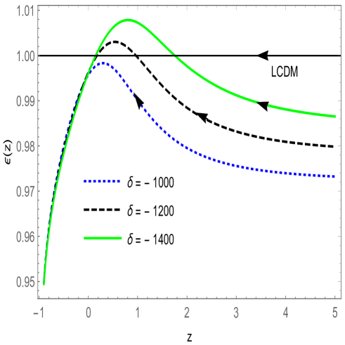
Figure 5: Graph of $\epsilon(z)$ versus redshift z, for non- interacting RHDE with Hbbble radius as the IR cutoff. Here, $H(z=0)=70$, $\Omega_{D}(z=0)=0.73$ and different values of $\delta$.

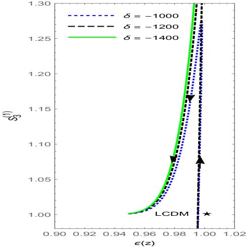
Figure 6: Graph of $S_{3}^{(1)}$ versus $\epsilon(z)$, for non- interacting RHDE with Hbbble radius as the IR cutoff. Here, $H(z=0)=67$, $\Omega_{m}(z=0)=0.26$, $R=10000$ and different values of $\delta$ (upper panel) and $H(z=0)=67$, $\Omega_{m}(z=0)0.26$, $\delta=-600$ and different values of R (below panel).

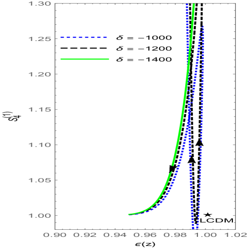
Figure 7: Graph of $S_{4}^{(1)}$ versus $\epsilon(z)$, for non- interacting RHDE with Hbbble radius as the IR cutoff. Here, $H(z=0)=70$, $\Omega_{D}(z=0)=0.73$ and different values of $\delta$.

IV.2 Growth rate of perturbations

The fractional growth parameter $\epsilon(z)$ ref76 ; ref77 is determined as

$$\epsilon(z)=\frac{f(z)}{f_{\text{$\Lambda$CDM}}(z)}$$ (25)

Here $f(z)=\frac{d\log\delta}{d\log a}$ is the growth rate of structure. Here, $\delta=\frac{\delta\rho_{m}}{\rho_{m}}$, with $\delta\rho_{m}$ and $\rho_{m}$ being the the density perturbation and energy density of matter (including CDM and baryons), respectively. If the perturbation is in the linear fashion and without any interaction between DM and DE, then we can say that the equation of perturbation at late times can be:

$$\ddot{\delta}+2\dot{\delta}H=4\pi\delta G\rho_{m}$$ (26)

Here, Newton’s gravitational constant is represented by $G$. So, the approx growth rate of linear density perturbation can be reflected by ref78 :

$$f(z)\simeq\Omega_{m}(z)^{\gamma}$$ (27)

$\gamma(z)=\frac{\left(3\left(1-\omega_{D}\right)\left(1-\frac{3\omega_{D}}{2}\right)\right)\left(1-\Omega_{m}(z)\right)}{125\left(1-\frac{6\omega_{D}}{5}\right){}^{3}}$ +

$$\frac{3}{5-\frac{\omega_{D}}{1-\omega_{D}}}$$ (28)

where $\Omega_{m}(z)=\frac{\rho_{m}(z)}{3H(z)^{2}M_{p}^{2}}$, the fractional density of matter, $\Omega$ is constant or varies slowly with time. $\epsilon(z)$ = 1 and $\gamma\simeq 0.55$ are the values for the $\Lambda$CDM model ref78 ; ref79 . For other models $\epsilon(z)$ exhibits differences from $\Lambda$CDM which would be the possible reason for its use as a diagnostic. By applying the composite null diagnostic ${CND}\equiv\left\{S_{n,}\epsilon\right\}$ where $\left\{S_{n,}\epsilon\right\}=\{1,1\}$ for $\Lambda$CDM, we can make use of both matter perturbational as well as geometrical information of cosmic evolution. While, we can analyze and present only one-side information of cosmic evolution by using one single diagnostic tool.

For the diagnose of diverse theoretical DE models, the evolution of the fractional growth parameter $\epsilon(z)$ is analysed. The evolutionary trajectories of $\epsilon(z)$ versus redshift $z$ for a spatially homogeneous and an isotropic flat FRW Universe of RHDE model by considering different values of $\delta$ are plotted in Fig. 5. It is observed that the evolutionary trajectories of $\epsilon(z)$ evolves below the $\Lambda$CDM line $\epsilon(z)=1$ and the curves separate well at the high red-shift region. The curves for $\delta$ = - 1200, $\delta$ = - 1400 are monotonically increasing and form convex vertices by crossing the $\Lambda$CDM line from past to present. The evolutionary trajectories of $\epsilon(z)$ for $\delta$ = - 1000, behaves in the same way but it does not cross the $\Lambda$CDM line. Presently, these curves are degenerated together and decrease monotonically for the low red-shift region.

Fig. 6 shows the evolutionary trajectories of $\left\{S_{3}^{(1)},\epsilon\right\}$ of RHDE model by considering different values of $\delta$. Where star symbol denotes the $\Lambda$CDM model $\left\{S_{3}^{(1)}=1,\epsilon=1\right\}$. From figure we observe that, curve evolves near $\Lambda$CDM model and monotonically increases and forms convex vertices and finally all these curves degenerated together to the line $S_{3}^{(1)}=1$ at low red-shift region.

Fig. 7 is the the evolutionary trajectories of the CND pair $\left\{S_{4}^{(1)},\epsilon\right\}$ for the RHDE model by considering different values of $\delta$ (upper panel) and R (below panel). The evolutionary trajectories of $\left\{S_{4}^{(1)},\epsilon\right\}$ shows similar characteristic as the curves of $\left\{S_{3}^{(1)},\epsilon\right\}$. These results shows that adopting different values of $\delta$ has quantitative impacts and the deviation from $\Lambda$CDM can be seen in this figure.

The evolutionary trajectories of the CND pair $\left\{S_{4}^{(1)},\epsilon\right\}$ for the RHDE model by considering different values of $\delta$ are depicted by Fig. 7. The behaviour of $\left\{S_{4}^{(1)},\epsilon\right\}$ are similar to the $\left\{S_{3}^{(1)},\epsilon\right\}$. In the Research work of cosmology, the present values of the parameters keeps important. In this direction we calculated the the present values of parameters $S_{30}^{(1)}$, $S_{40}^{(1)}$ , and $\epsilon_{0}$ of the RHDE model by considering different values of $\delta$ and also the differences of them, for each case $\bigtriangleup S_{30}^{(1)}$ = $S_{30}^{(1)}$(max)- $S_{30}^{(1)}$(min), $\bigtriangleup S_{40}^{(1)}$ = $S_{40}^{(1)}$(max)- $S_{40}^{(1)}$(min), and $\bigtriangleup\epsilon_{0}$= $\epsilon_{0}$(max) - $\epsilon_{0}$(min), which is given in Table 1. We observe that $\bigtriangleup S_{40}^{(1)}=0.198776>\bigtriangleup S_{30}^{(1)}=0.145811$. We can see $\bigtriangleup S_{40}^{(1)}>\bigtriangleup S_{30}^{(1)}$, which means that the fourth-order derivative of the scale factor in comparison to third-order derivative, intensifies the degeneracy of present values. Therefore $S_{40}^{(1)}$ in comparison to $S_{30}^{(1)}$ gives more variance for different values of $\delta$ among the cosmic evolution of RHDE type of DE. Which helps us to distinguish different theoretical models.

V Conclusions

The paper uses the R$\acute{e}$nyi Holographic Dark Energy model in the framework of an isotropic and spatially homogeneous flat FRW Universe by considering different values of RHDE parameter $\delta$, where the infrared cut-off is taken care by the Hubble horizon. This can be summarized as

• In this paper, we examined the deviation of RHDE model from $\Lambda$CDM with statefinder hierarchy supplemented by the growth rate of perturbations.

• The statefinder hierarchy $S_{3}^{(1)}$, $S_{3}^{(2)}$, $S_{4}^{(1)}$ and $S_{4}^{(2)}$, which contain the third and fourth derivatives of the scale factor, have been plotted versus red-shift z. The evolutionary trajectories of $S_{3}^{(1)}$ evolve below the $\Lambda$CDM line while $S_{4}^{(1)}$ evolves from above the $\Lambda$CDM line. The separation of the curvilinear shape of both parameters is more distinct in the region $0\leq z\leq 3$ for different values of $\delta$. The evolutionary trajectories of $S_{3}^{(2)}$ evolves above the $\Lambda$CDM line and crosses the $\Lambda$CDM line but $S_{4}^{(1)}$ evolves below the $\Lambda$CDM line and never crosses the $\Lambda$CDM line. All parameters degenerated closely together into $\Lambda$CDM line, at the low-redshift region.
  

• We have also examines the growth rate of structure $\epsilon(z)$ by plotting it versus red-shift z along with the combination of statefinder hierarchy $S_{n}$. The evolutionary trajectories of $\epsilon(z)$ degenerated together and decrease monotonically for low red-shift region. The curves of $\epsilon(z)$ separate well at high red-shift region for different values of $\delta$. The evolutionary trajectories of $\left\{S_{3}^{(1)},\epsilon\right\}$. and $\left\{S_{4}^{(1)},\epsilon\right\}$, shows the same deviation from $\Lambda$CDM model of RHDE model for all values of $\delta$.
  

• For alleviating the degeneracy existing in other statefinder parameters for DE models, comparison of the present-value differences of the parameters $S_{30}^{(1)}$, $S_{40}^{(1)}$ plays an important role. By using CND, we can discriminate RHDE model from $\Lambda$CDM. Since $\bigtriangleup S_{40}^{(1)}>\bigtriangleup S_{30}^{(1)}$, hence we can say that the fourth-order hierarchy of statefinder is a better choice than the third-order hierarchy for the RHDE model. Therefore, the above investigation concludes that the higher-order statefinder hierarchy, with the growth rate of perturbations, can differentiate the RHDE model from the $\Lambda$CDM model and also from itself with different parameter values.
  

  We hope that in future high precision observations, for example, SNAP-type investigation can be equipped for deciding the cosmological parameters exactly and consequently identify the correct cosmological model and closer to understand the properties of the RHDE model.

References

- (1) A. G. Riess et al. [Supernova Search Team], “Observational evidence from supernovae for an accelerating universe and a cosmological constant,” Astron. J. 116 (1998) 1009 doi:10.1086/300499
- (2) S. Perlmutter et al. [Supernova Cosmology Project Collaboration], “Measurements of and from 42 high redshift supernovae,” Astrophys. J. 517 (1999) 565 doi:10.1086/307221
- (3) https://www.lsst.org/
- (4) https://www.darkenergysurvey.org/
- (5) https://wfirst.gsfc.nasa.gov/
- (6) http://desi.lbl.gov/
- (7) N. Aghanim et al. [Planck Collaboration], arXiv:1807.06209 [astro-ph.CO].
- (8) L. Verde, T. Treu and A. G. Riess, arXiv:1907.10625 [astro-ph.CO].
- (9) S. Capozziello, R. D’Agostino and O. Luongo, “Extended Gravity Cosmography,” Int. J. Mod. Phys. D 28 (2019) no.10, 1930016 doi:10.1142/S0218271819300167
- (10) G. B. Zhao et al., “Dynamical dark energy in light of the latest observations,” Nat. Astron. 1 (2017) no.9, 627 doi:10.1038/s41550-017-0216-z
- (11) I. Sendra and R. Lazkoz, “SN and BAO constraints on (new) polynomial dark energy parametrizations: current results and forecasts,” Mon. Not. Roy. Astron. Soc. 422 (2012) 776 doi:10.1111/j.1365-2966.2012.20661.x
- (12) G. B. Zhao, D. Bacon, R. Maartens, M. Santos and A. Raccanelli, arXiv:1501.03840 [astro-ph.CO].
- (13) C. Escamilla-Rivera, “Status on bidimensional dark energy parameterizations using SNe Ia JLA and BAO datasets,” Galaxies 4 (2016) no.3, 8 doi:10.3390/galaxies4030008
- (14) M. Rezaei, M. Malekjani, S. Basilakos, A. Mehrabi and D. F. Mota, “Constraints to Dark Energy Using PADE Parameterizations,” Astrophys. J. 843 (2017) no.1, 65 doi:10.3847/1538-4357/aa7898
- (15) C. Escamilla-Rivera and S. Capozziello, “Unveiling cosmography from the dark energy equation of state,” Int. J. Mod. Phys. D 28 (2019) no.12, 1950154 doi:10.1142/S0218271819501542
- (16) J. Alberto Vazquez, M. Bridges, M. P. Hobson and A. N. Lasenby, “Reconstruction of the Dark Energy equation of state,” JCAP 1209 (2012) 020 doi:10.1088/1475-7516/2012/09/020
- (17) L. G. Jaime, L. Patiño and M. Salgado, “Note on the equation of state of geometric dark-energy in f(R) gravity,” Phys. Rev. D 89 (2014) no.8, 084010 doi:10.1103/PhysRevD.89.084010
- (18) R. Lazkoz, M. Ortiz-Baños and V. Salzano, “ gravity modifications: from the action to the data,” Eur. Phys. J. C 78 (2018) no.3, 213 doi:10.1140/epjc/s10052-018-5711-6
- (19) M. Seikel, C. Clarkson and M. Smith, “Reconstruction of dark energy and expansion dynamics using Gaussian processes,” JCAP 1206 (2012) 036 doi:10.1088/1475-7516/2012/06/036
- (20) A. Montiel, R. Lazkoz, I. Sendra, C. Escamilla-Rivera and V. Salzano, “Nonparametric reconstruction of the cosmic expansion with local regression smoothing and simulation extrapolation,” Phys. Rev. D 89 (2014) no.4, 043007 doi:10.1103/PhysRevD.89.043007
- (21) B. Ratra and P. J. E. Peebles, “Cosmological Consequences of a Rolling Homogeneous Scalar Field,” Phys. Rev. D 37 (1988) 3406. doi:10.1103/PhysRevD.37.3406
- (22) C. Armendariz-Picon, V. F. Mukhanov and P. J. Steinhardt, “A Dynamical solution to the problem of a small cosmological constant and late time cosmic acceleration,” Phys. Rev. Lett. 85 (2000) 4438 doi:10.1103/PhysRevLett.85.4438
- (23) S. Capozziello, “Curvature quintessence,” Int. J. Mod. Phys. D 11 (2002) 483 doi:10.1142/S0218271802002025
- (24) L. G. Jaime, M. Jaber and C. Escamilla-Rivera, “New parametrized equation of state for dark energy surveys,” Phys. Rev. D 98 (2018) no.8, 083530 doi:10.1103/PhysRevD.98.083530
- (25) L. Susskind, “The World as a hologram,” J. Math. Phys. 36 (1995) 6377 doi:10.1063/1.531249
- (26) P. Horava and D. Minic, “Probable values of the cosmological constant in a holographic theory,” Phys. Rev. Lett. 85 (2000) 1610 doi:10.1103/PhysRevLett.85.1610
- (27) S. D. Thomas, “Holography stabilizes the vacuum energy,” Phys. Rev. Lett. 89 (2002) 081301. doi:10.1103/PhysRevLett.89.081301
- (28) S. D. H. Hsu, “Entropy bounds and dark energy,” Phys. Lett. B 594 (2004) 13 doi:10.1016/j.physletb.2004.05.020
- (29) M. Li, “A Model of holographic dark energy,” Phys. Lett. B 603 (2004) 1 doi:10.1016/j.physletb.2004.10.014
- (30) R. G. Cai, “A Dark Energy Model Characterized by the Age of the Universe,” Phys. Lett. B 657 (2007) 228 doi:10.1016/j.physletb.2007.09.061
- (31) H. Wei and R. G. Cai, “A New Model of Agegraphic Dark Energy,” Phys. Lett. B 660 (2008) 113 doi:10.1016/j.physletb.2007.12.030
- (32) C. Gao and F. Wu et al., “A Holographic Dark Energy Model from Ricci Scalar Curvature,” Phys. Rev. D 79 (2009) 043511. doi:10.1103/PhysRevD.79.043511
- (33) C. Tsallis and L. J. L. Cirto, “Black hole thermodynamical entropy,” Eur. Phys. J. C 73 (2013) 2487 doi:10.1140/epjc/s10052-013-2487-6
- (34) C. Tsallis, “Possible Generalization of Boltzmann-Gibbs Statistics,” J. Statist. Phys. 52 (1988) 479. doi:10.1007/BF01016429
- (35) A.Rnyi , in Proceedings of the 4th Berkely Symposium on Mathematics, Statistics and Probability (University California Press, Berkeley, CA, 1961) pp. 547–561.
- (36) B.D. Sharma and D.P. Mittal, “ New non-additive measures of entropy for discrete probability distributions,” J. Math. Sci.10 (1975) 28-40; B.D. Sharma, D.P. Mittal, J. Comb. Inf. Syst. Sci. 2 (1977) 122.
- (37) M. Tavayef, A. Sheykhi, K. Bamba and H. Moradpour, “Tsallis Holographic Dark Energy,” Phys. Lett. B 781 (2018) 195 doi:10.1016/j.physletb.2018.04.001
- (38) M. Abdollahi Zadeh, A. Sheykhi and H. Moradpour, “Tsallis Agegraphic Dark Energy Model,” Mod. Phys. Lett. A 34 (2019) no.11, 1950086 doi:10.1142/S021773231950086X
- (39) H. Moradpour, S. A. Moosavi, I. P. Lobo, J. P. Morais Graça, A. Jawad and I. G. Salako, “Thermodynamic approach to holographic dark energy and the Rényi entropy,” Eur. Phys. J. C 78 (2018) no.10, 829 doi:10.1140/epjc/s10052-018-6309-8
- (40) A. Sayahian Jahromi, S. A. Moosavi, H. Moradpour, J. P. Morais Graça, I. P. Lobo, I. G. Salako and A. Jawad, “Generalized entropy formalism and a new holographic dark energy model,” Phys. Lett. B 780 (2018) 21 doi:10.1016/j.physletb.2018.02.052
- (41) A. Jawad, K. Bamba, M. Younas, S. Qummer and S. Rani, “Tsallis, Rényi and Sharma-Mittal Holographic Dark Energy Models in Loop Quantum Cosmology,” Symmetry 10 (2018) no.11, 635. doi:10.3390/sym10110635
- (42) S. Nojiri, S. D. Odintsov and E. N. Saridakis,“Modified cosmology from extended entropy with varying exponent,” Eur. Phys. J. C 79 (2019) 242.
- (43) Q. Huang, H. Huang, J. Chen, L. Zhang and F. Tu, “Stability analysis of a Tsallis holographic dark energy model,” Class. Quant. Grav. 36, no. 17, (2019) 175001. S. Ghaffari, H. Moradpour, I. P. Lobo, J. P. Morais Graça and V. B. Bezerra, “Tsallis holographic dark energy in the Brans–Dicke cosmology,” Eur. Phys. J. C 78 (2018) no.9, 706 doi:10.1140/epjc/s10052-018-6198-x
- (44) E. N. Saridakis, K. Bamba, R. Myrzakulov and F. K. Anagnostopoulos, “Holographic dark energy through Tsallis entropy,” JCAP 1812 (2018) 012 doi:10.1088/1475-7516/2018/12/012
- (45) V. C. Dubey, S. Srivastava, U. K. Sharma and A. Pradhan, “Tsallis holographic dark energy in Bianchi-I Universe using hybrid expansion law with -essence,” Pramana 93 (2019) no.5, 78. doi:10.1007/s12043-019-1843-y
- (46) E. Sadri, “Observational constraints on interacting Tsallis holographic dark energy model,” Eur. Phys. J. C 79 (2019) no.9, 762 doi:10.1140/epjc/s10052-019-7263-9
- (47) E. M. Barboza, Jr., R. d. C. Nunes, E. M. C. Abreu and J. Ananias Neto, “Dark energy models through nonextensive Tsallis’ statistics,” Physica A 436 (2015) 301 doi:10.1016/j.physa.2015.05.002
- (48) Golanbari, T., Saaidi, K., Karimi, P. (2020). ” Rnyi entropy and the holographic dark energy in flat space time”. arXiv preprint arXiv:2002.04097.
- (49) Sharma, U. K., Dubey, V. C. (2020). ”Interacting Rnyi holographic dark energy with parametrization on the interaction term”. arXiv preprint arXiv:2001.02368.
- (50) S. Ghaffari, A. H. Ziaie, V. B. Bezerra and H. Moradpour, “Inflation in the Rnyi cosmology,” Mod. Phys. Lett. A 35 (2019) no.01, 1950341 doi:10.1142/S0217732319503413
- (51) V. C. Dubey, et al. “Tsallis holographic dark energy Models in axially symmetric space time.” Int. J. Geom. Methods Mod. Phys. 17 1 (2020) 2050011.
- (52) Y. Aditya, S. Mandal, P. K. Sahoo and D. R. K. Reddy, “Observational constraint on interacting Tsallis holographic dark energy in logarithmic Brans–Dicke theory,” Eur. Phys. J. C 7912, 1020 (2019).
- (53) A. Iqbal and A. Jawad, “Tsallis, Renyi and Sharma–Mittal holographic dark energy models in DGP brane-world,” Phys. Dark Univ. 26 (2019) 100349. doi:10.1016/j.dark.2019.100349
- (54) M. Arabsalmani and V. Sahni, “The Statefinder hierarchy: An extended null diagnostic for concordance cosmology,” Phys. Rev. D 83 (2011) 043501. doi:10.1103/PhysRevD.83.043501
- (55) J. F. Zhang and J. L. Cui et al., “Diagnosing holographic dark energy models with statefinder hierarchy,” Eur. Phys. J. C 74 (2014) no.10, 3100. doi:10.1140/epjc/s10052-014-3100-3
- (56) R. Myrzakulov and M. Shahalam, “Statefinder hierarchy of bimetric and galileon models for concordance cosmology,” JCAP 1310 (2013) 047 doi:10.1088/1475-7516/2013/10/047
- (57) J. F. Zhang, J. L. Cui and X. Zhang, “Diagnosing holographic dark energy models with statefinder hierarchy,” Eur. Phys. J. C 74 (2014) no.10, 3100 doi:10.1140/epjc/s10052-014-3100-3
- (58) J. L.Cui, et al., ”A closer look at interacting dark energy with statefinder hierarchy and growth rate of structure”. JCAP 09(2015) 024.
- (59) J. Li, R. Yang and B. Chen, “Discriminating dark energy models by using the statefinder hierarchy and the growth rate of matter perturbations,” JCAP 1412 (2014) 043 doi:10.1088/1475-7516/2014/12/043
- (60) V. Acquaviva and A. Hajian et al., “Next Generation Redshift Surveys and the Origin of Cosmic Acceleration,” Phys. Rev. D 78 (2008) 043514. doi:10.1103/PhysRevD.78.043514
- (61) V. Acquaviva and E. Gawiser, “How to Falsify the GR+LambdaCDM Model with Galaxy Redshift Surveys,” Phys. Rev. D 82 (2010) 082001. doi:10.1103/PhysRevD.82.082001
- (62) R. Myrzakulov and M. Shahalam, “Statefinder hierarchy of bimetric and galileon models for concordance cosmology,” JCAP 1310 (2013) 047. doi:10.1088/1475-7516/2013/10/047
- (63) J. Li and R. Yang et al., “Discriminating dark energy models by using the statefinder hierarchy and the growth rate of matter perturbations,” JCAP 1412 (2014) 043. doi:10.1088/1475-7516/2014/12/043
- (64) Y. Hu and M. Li et al., “Impacts of different SNLS3 light-curve fitters on cosmological consequences of interacting dark energy models,” Astron. Astrophys. 592 (2016) A101. doi:10.1051/0004-6361/201526946
- (65) A. Mukherjee, N. Paul and H. K. Jassal, “Constraining the dark energy statefinder hierarchy in a kinematic approach,” JCAP 1901 (2019) 005 doi:10.1088/1475-7516/2019/01/005
- (66) J. L. Cui, L. Yin, L. F. Wang, Y. H. Li and X. Zhang, “A closer look at interacting dark energy with statefinder hierarchy and growth rate of structure,” JCAP 1509 (2015) 024 doi:10.1088/1475-7516/2015/09/024
- (67) L. Zhou and S. Wang, “Diagnosing HDE model with statefinder hierarchy and fractional growth parameter,” Sci. China Phys. Mech. Astron. 59 (2016) no.7, 670411 doi:10.1007/s11433-016-0038-9
- (68) Majumdar, A., Chattopadhyay, S., ”A study of modified holographic Ricci dark energy in the framework of f (T) modified gravity and its statefinder hierarchy”. Can. J. Phys. 97(5) ( 2018) 477-486.
- (69) Zhao, Z., Wang, S., ”Diagnosing holographic type dark energy models with the Statefinder hierarchy, composite null diagnostic and pair”. China Phys. Mech. Astron. 61(3) (2018) 039811.
- (70) Yu, F., et al., ”Statefinder hierarchy exploration of the extended Ricci dark energy”. Eur. Phys. J. C 75(6)(2015)274.
- (71) Mukherjee, A., Paul, N., Jassal, H. K., 2019. Constraining the dark energy statefinder hierarchy in a kinematic approach. JCAP 2019(01), 005.
- (72) Zhang, N., et al. 2019. Diagnosing the interacting Tsallis Holographic Dark Energy models. arXiv preprint arXiv:1905.04299.
- (73) Srivastava, V. and Sharma.U. K., ”Statefinder hierarchy for Tsallis holographic dark en- ergy.” New Astronomy (2020): 101380.
- (74) A.Rnyi , in Proceedings of the 4th Berkely Symposium on Mathematics, Statistics and Probability (University California Press, Berkeley, CA, 1961) pp. 547–561.
- (75) V. Sahni and A. Shafieloo et al., “Two new diagnostics of dark energy,” Phys. Rev. D 78 (2008) 103502. doi:10.1103/PhysRevD.78.103502
- (76) V. Acquaviva and A. Hajian et al., “Next Generation Redshift Surveys and the Origin of Cosmic Acceleration,” Phys. Rev. D 78 (2008) 043514. doi:10.1103/PhysRevD.78.043514
- (77) V. Acquaviva and E. Gawiser, “How to Falsify the GR+LambdaCDM Model with Galaxy Redshift Surveys,” Phys. Rev. D 82 (2010) 082001. doi:10.1103/PhysRevD.82.082001
- (78) L. M. Wang and P. J. Steinhardt, “Cluster abundance constraints on quintessence models,” Astrophys. J. 508 (1998) 483. doi:10.1086/306436
- (79) E. V. Linder, “Cosmic growth history and expansion history,” Phys. Rev. D 72 (2005) 043529. doi:10.1103/PhysRevD.72.043529