Exotic photonic molecules via Lennard-Jones-like potentials

Abstract

Ultracold systems offer an unprecedented level of control of interactions between atoms. An important challenge is to achieve a similar level of control of the interactions between photons. Towards this goal, we propose a realization of a novel Lennard-Jones-like potential between photons coupled to the Rydberg states via electromagnetically induced transparency (EIT). This potential is achieved by tuning Rydberg states to a Förster resonance with other Rydberg states. We consider few-body problems in 1D and 2D geometries and show the existence of self-bound clusters (“molecules”) of photons. We demonstrate that for a few-body problem, the multi-body interactions have a significant impact on the geometry of the molecular ground state. This leads to phenomena without counterparts in conventional systems: For example, three photons in 2D preferentially arrange themselves in a line-configuration rather than in an equilateral-triangle configuration. Our result opens a new avenue for studies of many-body phenomena with strongly interacting photons.

Atomic, molecular, and optical platforms allow for precise control and wide-ranging tunability of system parameters using external fields. Interactions between atoms can be controlled via Feshbach resonances enabling studies of the BCS-BEC crossover Bloch2008 ; Chin2010 or via highly-excited Rydberg states giving rise to frustrated magnetism VanBijnen2015 , topological order Glaetzle2015 , and other exotic phases Grass2018 . Interactions between single photons in vacuum or conventional transparent materials are negligible; however, they can be enhanced by strongly coupling photons to specially engineered matter Chang2014 . An open challenge is to achieve a similar level of tunability for strongly interacting photons as demonstrated for atoms. Such tunability could lead to applications in photonic quantum information processing, metrology, sensing, as well as exotic photonic phases of matter Chang2015 .

A promising platform to achieve this goal are Rydberg polaritons, for which interactions between Rydberg states are mapped onto photons via EIT Fleischhauer2000 ; Lukin2001 ; Friedler2005 . The effective interactions between photons are not only strong Pritchard2010 , but also saturate to a constant value Firstenberg2013 ; Bienias2014 ; Bienias2016a ; Bienias2020 for distances shorter than the blockade radius $r_{b}\sim 10\,\mu$m, which usually is much greater than the wavelength of the photons. These properties have enabled several theoretical proposals and experimental realizations related to quantum information processing, such as gates Tiarks2019 ; Tiarks2016 , transistors Tiarks2014 ; Gorniaczyk2014 ; Gorniaczyk2016 , and non-classical states of light Dudin2012 ; Peyronel2012 ; OrnelasHuerta2020 ; Bienias2020c .

Up to now, the field of dispersive Rydberg-EIT has predominantly concentrated on the effective interactions between polaritons proportional to $1/(r_{b}^{6}+r^{6})$, which change monotonically as a function of separation $r$. Additional work has explored: lossy foot1 Coulomb bound states; and bound states via interactions mediated by 1D photonic crystals Douglas2016 . Here, we propose a novel method to tune the shape of the divergence-free interactions Maghrebi2015c in 1D and 2D between photons propagating through the Rydberg medium.

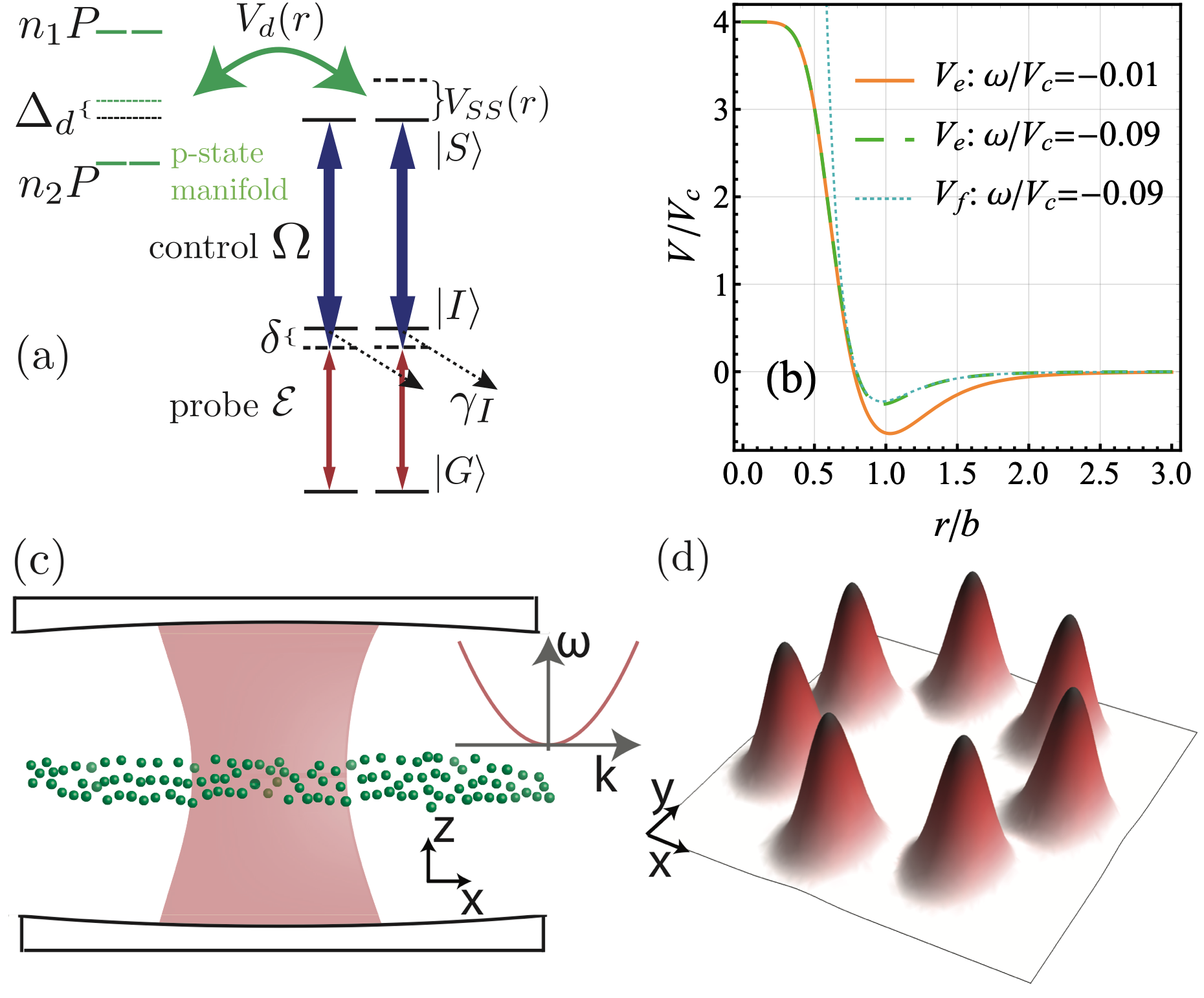
Figure 1: Using magnetic fields, we tune $\left|SS\right\rangle$ (characterized by principal quantum number $n$) close to the resonance (deviation from resonance denoted by $\Delta_{d}$) with the $P_{1}P_{2}$ state having $n_{1}$ $=$ $n$ and $n_{2}$ $=$ $n-1$. (b) This gives rise to the effective molecular potential $V_{e}$ plotted for $\Delta_{d}/V_{c}$ $=$ $0.03$ used also in Fig. 2(b). By working with $|V_{\rm\scriptscriptstyle min}|\ll 1/|\bar{\chi}|$, this potential around the local minimum is nearly equal to $V_{f}$ (i.e. is not modified by $\bar{\chi}$), see blue dotted vs green dashed curve. (c) A quasi-2D cloud of atoms placed in the center of a multi-mode cavity. The mode structure of the cavity gives an effective mass for free particles moving in 2D. The inset shows the resulting quadratic photonic dispersion relation. For strong nonlinearities, this setup gives rise to few- and many-body self-bound clusters of light in 2D, e.g arranged on a ring, which is illustrated in (d) for seven photons.

We achieve this using Förster resonances, which are a useful tool to control interactions between atoms  Lukin2001 ; Afrousheh2004 ; Bohlouli-Zanjani2007 ; Vogt2006 ; Ryabtsev2010 ; Reinhard2008 ; Nipper2012 ; Ravets2015 ; Pelle2016 ; Beterov2015 . Application of these resonances to quantum optics with Rydberg polaritons was studied in the context of Rydberg atom imaging Gunter2012 ; Olmos2011 ; Gunter2013 and an all-optical transistor Gorniaczyk2016 ; Tiarks2014 . We demonstrate that with an appropriate choice of states and couplings, we can achieve a Lennard-Jones-like potential between photons, which has a global minimum at a finite distance [see Fig. 1(b)]. We show the existence of bound states in 1D and 2D for two photons interacting via this molecular potential, and further discuss multi-photon self-bound clusters (molecules) of photons [see Fig. 1(d)].

In the previous studies of shallow Firstenberg2013 and deep Bienias2014 bound states, the photons interacted via a soft-core potential and therefore preferred to overlap. This precluded the formation of more complex molecular-like structures that is possible in our proposal. The many-photon clusters studied here resemble photonic crystalline features studied in 1D  Otterbach2013 ; Chang2008 and 2D  Sommer2015 . However, the latter proposals are based on strong repulsion and therefore, without the external trapping potential, the crystals become unstable in contrast to our work proposing self-bound clusters.

One of the unconventional properties of Rydberg-EIT is strong three- and higher-body interactions between polaritons Jachymski2016 ; Gullans2016 ; Kalinowski2020b . These strong three-body interactions impact the energies of three-body bound states Liang2018 . Here, we show that Förster resonances in combination with Rydberg-EIT lead to another source of many-body forces. These additional forces give rise to new phenomena. For example, it is energetically favorable to have three polaritons in a line, rather than in a triangular configuration.

System

Throughout, we focus on photons evolving in 1D and 2D multimode cavities Sommer2015 ; Sommer2016 ; Schine2016 ; Jia2018 ; Clark2019b , Fig. 1(c), described by the single-particle Hamiltonian Sommer2015 ; Parigi2012 ; Stanojevic2013 ; Georgakopoulos2018b ; Litinskaya2016 ; Grankin2014 ($\hbar$ $=$ $1$)

$$H_{1} = \int d{\bf r}\begin{pmatrix}\hat{\mathcal{E}}\\ \hat{I}\\ \hat{S}\end{pmatrix}^{\dagger}\!\left(\begin{array}[]{ccc}-i\kappa+T&g&0\\ g&\Delta&\Omega\\ 0&\Omega&-i\gamma_{S}\\ \end{array}\right)\begin{pmatrix}\hat{\mathcal{E}}\\ \hat{I}\\ \hat{S}\end{pmatrix},$$ (4)

where $\hat{\mathcal{E}}$ is the field operator describing the photonic mode, whereas $\hat{I}$ and $\hat{S}$ describe intermediate- and Rydberg-state collective spin excitations, respectively Fleischhauer2000 . $2\kappa$ is the cavity loss rate, $\Delta$ $=$ $\delta-i\gamma_{I}$ is the complex single-photon detuning, $2\gamma_{I}$ is the atomic intermediate state decay rate, $2\gamma_{S}$ is the Rydberg level decay rate, $g$ is the single-photon coupling, and $\Omega$ is the Rabi frequency of the control drive. The kinetic energy of photons is described in 1D and 2D via $T$ $=$ $-\frac{\nabla^{2}}{2m_{\rm\scriptscriptstyle ph}}$, where $m_{\rm\scriptscriptstyle ph}$ is the photon mass defined by the cavity parameters. Note that our approach can be easily generalized to a 1D free-space geometry, which is discussed below. The Hamiltonian  in Eq. 4 can be diagonalized and leads to two bright and one dark polariton branches Bienias2014 . Well within the EIT window Petrosyan2011 and in the limit of $\Omega\ll g$ (assumed throughout), the dark-state polariton $\hat{D}$ takes the form $\hat{D}\sim\hat{S}-\frac{\Omega}{g}\hat{\mathcal{E}}$. To leading order, the dark-state polariton losses are $\frac{\Omega^{2}}{g^{2}}\kappa+\gamma_{S}$ and are negligible for the evolution times considered in this Letter. For simplicity we shall assume $|\delta|\gg\gamma_{I}$, and therefore neglect the imaginary part of $\Delta$. The dispersion of $\hat{D}$ is inherited from the photonic component and therefore described via an enhanced mass equal to $m$ $=$ $\frac{g^{2}}{\Omega^{2}}m_{\rm\scriptscriptstyle ph}$.

The interactions for conventional dark-state polaritons are inherited from the van der Waals (vdW) interactions between Rydberg states Mohapatra2008 ; Friedler2005 described by the quartic term proportional to $\hat{S}^{\dagger}({\bf r})\hat{S}^{\dagger}({\bf r}^{\prime})V_{SS}({\bf r}-{\bf r}^{\prime})\hat{S}({\bf r}^{\prime})\hat{S}({\bf r})$. However, close to the Förster resonance, the physics becomes more subtle because at least two strongly-interacting pairs of states are involved. To build intuition, we first study the two-body problem.

Effective Lennard-Jones-like potential

In the past, Förster resonances were used in Rydberg-EIT transistor experiments Gorniaczyk2016 ; Tiarks2014 which used two $S$-states with different principal quantum numbers for the gate and source photons. Here, we are interested in few- and many-body physics and therefore use a single $nS$-state foot2 .In this case, there is no true Förster resonance at zero external fields Walker2008 , but there is an approximate one $nS+nS\rightarrow nP+(n-1)P$. We consider $J$ $=$ $1/2,m_{J}$ $=$ $1/2$ $S$-states and $J$ $=$ $3/2,m_{J}$ $=$ $3/2$ $P$-states and tune them to near resonance Gorniaczyk2016 [see Fig. 1(a)] using a strong magnetic field (defining the quantization axis) perpendicular to the atomic cloud foot3 .

Under these conditions, there are three relevant pairs of Rydberg states $\{SS,P_{1}P_{2},P_{2}P_{1}\}$ with interactions between them described by

$$\left(\begin{array}[]{ccc}V_{SS}&V_{d}&V_{d}\\ V^{*}_{d}&V_{PP}+\Delta_{d}&V_{PP,\text{off}}\\ V^{*}_{d}&V_{PP,\text{off}}&V_{PP}+\Delta_{d}\\ \end{array}\right),$$ (8)

where $\Delta_{d}$ $=$ $E_{P_{1}}+E_{P_{2}}-2E_{S}$ is the Förster defect and $V_{d}$ $=$ $C_{3}e^{i2\phi_{12}}/r^{3}$ is a dipolar interaction with the polar angle $\phi_{12}$ describing the direction of the relative distance ${\bf r}$ $=$ ${\bf r}_{1}-{\bf r}_{2}$ between the first and second excitation, with $r$ $=$ $|{\bf r}|$. In general, $|V_{d}|$ could have an additional azimuthal-angle dependence, which is not present for the 1D and 2D geometries considered here. $V_{SS}$ $=$ $C_{SS}/r^{6},V_{PP}$ $=$ $C_{PP}/r^{6}$ are diagonal vdW interactions foot4 , whereas $V_{PP,{\rm\scriptscriptstyle off}}$ $=$ $C_{PP,{\rm\scriptscriptstyle off}}/r^{6}$ is the off-diagonal vdW interaction between $P_{1}P_{2}$ and $P_{2}P_{1}$.

The conventional Rydberg-EIT two-body problem can be described using a set of nine coupled Maxwell-Bloch equations Gorshkov2011 ; Peyronel2012 ; Bienias2016 for $XY$ components of the two-body wavefunction, where $X,Y\in\{\mathcal{E},I,S\}$. Importantly, the $P_{2}P_{1}$ and $P_{1}P_{2}$ components are coupled to the conventional equations Peyronel2012 ; supplementCluster only via dipolar interactions $V_{d}$. This enables us to eliminate the $P_{2}P_{1}$ and $P_{1}P_{2}$ components (see supplement supplementCluster ) and leads to the standard equations of motion but where $V_{SS}$ is replaced by

$$\vspace{-0em}V_{f}(r)=\frac{C_{SS}}{r^{6}}-\frac{2\left(\frac{C_{3}}{r^{3}}\right)^{2}}{\Delta_{d}+\frac{C_{PP}+C_{PP,{\rm\scriptscriptstyle off}}}{r^{6}}-\omega}\vspace{-0.em}$$ (9)

with $\omega$ the total energy of the pair of polaritons. This potential [see Fig. 1(b)] can have a local minimum which intuitively comes from the interplay of the diagonal interactions $\sim 1/r^{6}$ and the off-diagonal couplings $\sim 1/r^{3}$: The latter terms dominate at large separation causing the potential curve $SS$ to be attractive, whereas at short distances the vdW interaction dominates and the potential is repulsive. This is in contrast to other molecular potentials Hollerith2019 ; Petrosyan2014 arising from the avoided crossings between potential curves. Based on $V_{f}$, using the approach developed in Ref. Bienias2014 , we arrive at the soft-core effective potential between polaritons

$$V_{e}({r})=\frac{V_{f}({r})}{1-\bar{\chi}V_{f}({r})},$$ (10)

where $\bar{\chi}$ $=$ $\frac{\Delta}{2\Omega^{2}}-\frac{1}{2\Delta}$ for the regime considered below. In contrast with conventional Rydberg-EIT, both the strength and shape of $V_{f}$ can be tuned using $\Delta_{d}$ and the choice of principal quantum numbers. In general, the depth $V_{\rm\scriptscriptstyle min}$ of the potential $V_{e}$ can be as large as its height equal to $-1/\bar{\chi}$. However, by assuming henceforth a shallow $V_{e}$ such that $V_{\rm\scriptscriptstyle min}\ll\omega_{c}\equiv 1/|\bar{\chi}|$, we can: (i) neglect dependence of $\bar{\chi}$ on $\omega$ because $\omega\sim V_{\rm\scriptscriptstyle min}$ Bienias2014 ; (ii) neglect the scattering to bright polaritons for a small center-of-mass momentum $K\ll k_{c}\equiv\frac{g^{2}}{c\Omega^{2}}\omega_{c}$ Bienias2014 assumed henceforth; (iii) neglect blockade-induced three-body interactions Jachymski2016 ; Gullans2016 .

Two-body problem

The two-body problem can be described using the wavefunction $\varphi(\bf{r})$ depending on the relative distance $\bf{r}$. $\varphi$ describes two dark-state polaritons, is proportional to $\mathcal{EE}\sim\mathcal{ES}+\mathcal{SE}$, and is the solution of the effective Schroedinger equation Bienias2014

$$\omega\varphi({\bf r})=\bigg{[}-\frac{\nabla^{2}}{m}+V_{e}({r},\Delta_{d},\omega)\bigg{]}\varphi(\bm{r}).$$ (11)

As discussed, we can neglect dependence of $\bar{\chi}$ on $\omega$, however, there is still dependence of $V_{f}$ on $\omega$, see Eq. (9), which we take into account in the numerics. The local minimum of $V_{e}$ exists for $C_{SS}\left(\omega-\Delta_{d}\right)+2C_{3}^{2}>0$. Considering $|\omega|\ll\Delta_{d}$ enables us to define the characteristic energy $\nu_{c}$ $=$ $2C_{3}^{2}/C_{SS}$ quantifying the range of $\Delta_{d}$ for which a bound state could exist. In addition, we define (for details see supplement) the characteristic length scale $b$ $=$ $\left({\left(\sqrt{2}+1\right)C_{PP}C_{SS}}/{C_{3}^{2}}\right)^{1/6}$ for the position of the local minimum, and $V_{c}$ $=$ ${2C_{3}^{2}}/{C_{PP}}$ quantifying the depth of the potential.

Next, we self-consistently find the solutions of Eq. (11) for different $\Delta_{d}$. In Fig. 2, we show solutions for the 1D limit of Eq. (11) for $V_{c}m\,b^{2}$ $=$ $40$, corresponding to $\text{OD}_{b}\,{\gamma_{I}}/{\delta}$ $=$ $0.9$, where OD${}_{b}\equiv\text{OD}\frac{b}{L}$ is an optical depth OD per $b$. The smaller the ratio $\Delta_{d}/V_{c}$ is, the deeper $V_{f}$ is and, therefore, the second (and even third) bound state can be seen in Fig. 2(a). The lowest bound state (green in  Fig. 2(b)) has a width smaller than the first excited bound state (orange), the latter having a single node around the local minimum of $V_{e}$ at $r$ $\approx$ $b$, Fig. 1(b). Both wavefunctions are strongly suppressed at short distances due to the strong repulsion for small $r$.

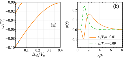
Figure 2: Results for ⁸⁷Rb, $n$ $=$ $120,$ $n_{1}$ $=$ $120,$ $n_{2}$ $=$ $119$, $\Omega<|\Delta|$, $V_{c}m\,b^{2}$ $=$ $40$, and $\omega_{c}$ $=$ $4V_{c}$, which is achieved by an appropriate choice of $\Omega$. (a) Bound-state energies as a function of $\Delta_{d}$ in units of $V_{c}$. (b) The wavefunctions for two lowest bound states with $\Delta_{d}/V_{c}$ $=$ $0.03$ (blue dots in (a)).

Three and more photons

For conventional few-body problems, it is usually a good approximation to assume that each pair of bodies interacts via a two-body potential. However, Rydberg polaritons are an unconventional platform enabling strong many-body interactions, as was shown for a soft-core potential $V_{e}$ in Refs Jachymski2016 ; Gullans2016 ; Liang2018 . In this Letter, we can neglect these higher-body interactions because states of interest are largely supported outside the repulsive core of the potential, and therefore, the three-body forces are strongly suppressed for $|\bar{\chi}V_{\rm\scriptscriptstyle min}|\ll 1$, Refs Jachymski2016 ; Gullans2016 ; Kalinowski2020b . However, we show that Förster resonances in combination with Rydberg-EIT lead to another source of many-body forces.

Even though the $SS$ channel is on resonance with two channels $P_{1}P_{2}$ and $P_{2}P_{1}$, the majority of the three-body physics can be well-described by a single effective channel $PP\sim P_{1}P_{2}+P_{2}P_{1}$ supplementCluster (note that all the numerics are performed without this approximation). The dipolar interaction between states $\{SSS,SPP,{PSP},{PPS}\}$ takes the form

$$\vspace{-0em}\left(\begin{array}[]{cccc}V_{S}&V_{d,23}&V_{d,13}&V_{d,12}\\ V^{*}_{d,23}&V_{{P,1}}+\Delta_{d}&W_{12}&W_{13}\\ V^{*}_{d,13}&W_{12}&V_{{P,2}}+\Delta_{d}&W_{23}\\ V^{*}_{d,12}&W_{13}&W_{23}&V_{{P,3}}+\Delta_{d}\\ \end{array}\right),\vspace{-0.em}$$ (12)

where $V_{P,i}$ $=$ $V_{PP}(r_{j}-r_{k})+V_{SP}(r_{i}-r_{j})+V_{SP}(r_{i}-r_{k})$ with $i\neq j,k$ and $j<k$ describes all vdW interactions between involved Rydbergs; $V_{S}$ is a sum of vdW interactions between all polaritons in $S$ state. $V_{d,ij}$ $=$ $\sqrt{2}C_{3}e^{i2\phi_{ij}}/|{\bf r}_{i}-{\bf r}_{j}|^{3}$ is the effective dipole interaction between $SS$ and $PP$. Analogously, $W_{ij}(r)$ $=$ $-\frac{1}{3}C_{3}/|{\bf r}_{i}-{\bf r}_{j}|^{3}$ describes the dipole interaction between $SP$ and $PS$. Without off-diagonal $W$ terms, we could eliminate all components containing $P$-states. However, due to these exchange terms, this is no longer possible, which is one of the reasons for the strong N-body forces.

Low-energy regime

The low energy assumption, $T_{i}\ll|V_{\rm\scriptscriptstyle min}|$ (where $T_{i}$ is the kinetic energy of the $i$th polariton), together with the already made assumption that $|V_{\rm\scriptscriptstyle min}|\ll\omega_{c}$, ensures that the dipolar interactions modify the internal composition of the dark states only weakly Otterbach2013 . Therefore, we can neglect the blockade effects on the effective interaction $V_{e}$ and dark-state polaritons. In the slow-light regime of $g\gg\Omega$, dark states $D$ have a negligible contribution from $\mathcal{E}$ and $I$ and mostly consist of Rydberg states. Hence, the dipolar Hamiltonian Eq. (12) maps directly onto dark-state polaritons $D$ and collective excitations $P$. That is, the full Hamiltonian describing the evolution of the three polaritons in the $\{DDD,DPP,{PDP},{PPD}\}$ basis is a sum of Eq. (12) with kinetic terms $\{T_{1}+T_{2}+T_{3},T_{1},T_{2},T_{3}\}$ on the diagonals.

Few-body bound states in the large-mass limit

To give additional insights into the role of few-body interactions in the many-body problem, in the following we neglect kinetic energy all together. This requires $V_{c}\gg 1/{m}b^{2}$ and therefore OD${}_{b}\gg\frac{\delta}{\gamma_{I}}$ .

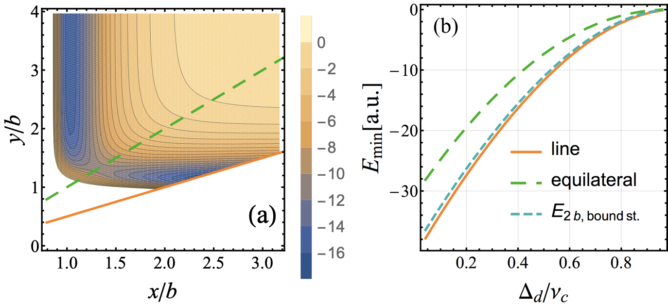
Figure 3: Self-consistent solution of Eq. (12) describing polaritons in the large-mass limit. (a) Three-body problem in the isosceles triangular configuration with edge lengths $y,y,x$. (b) Lowest energy as a function of $\Delta_{d}$ for line, regular-polygon, and dimer configurations for three bodies. Results are for ⁸⁷Rb with $n_{1},n_{2},n$ as in Fig. 2. Additionally, (a) is for $\Delta_{d}/\nu_{c}$ $=$ $0.4$.

Next, we numerically solve for the eigenstates of the two-channel version supplementCluster of the Hamiltonian Eq. (12) as a function of separations $r_{ij}$ in a 2D geometry. We find that it is preferable to have three polaritons in a line rather than in an equilateral-triangle configuration. Moreover, the configuration in which one photon is away from the dimer has lower energy than the equilateral-triangle configuration. This is demonstrated in Fig. 3(a-b) where (a) shows total energies for the polaritons being at the corners of an isosceles triangle and (b) shows that regardless of the value of $\Delta_{d}/\nu_{c}$, the line-configuration has the lowest energy foot5 .

Intuition behind the N-body force

For the three-body problem, even approximate analytical expressions for eigenstates of Eq. (12) are lengthy for arbitrary separations. Therefore, we use an equilateral-triangle configuration parametrized by edge length $r$ to obtain more intuition on the three-body forces. The energy $E$ being the lowest eigenvalue of Eq. (12) as a function of the separation $r$, for $E\ll\Delta_{d}$, takes the form

$$E=3\left(\frac{C_{SS}}{r^{6}}-\frac{2\left(\frac{\text{C}_{3}}{r^{3}}\right){}^{2}}{\Delta_{d}+\frac{C_{PP}+2C_{SP}}{r^{6}}-W(r)}\right).$$ (13)

From comparison of this expression with Eq. (9), we see that the denominator has two additional terms foot6 : (i) the vdW energy shift $2C_{SP}/r^{6}$, and (ii) the shift due to the off-diagonal dipolar interactions $W(r)<0$ foot7 . Both lead to the suppression of $E$, resulting in strong three-body repulsion which prevents configurations with three particles closely spaced. This gives rise to the novel ground state geometries presented in Fig. 3.

Multiple-body problem

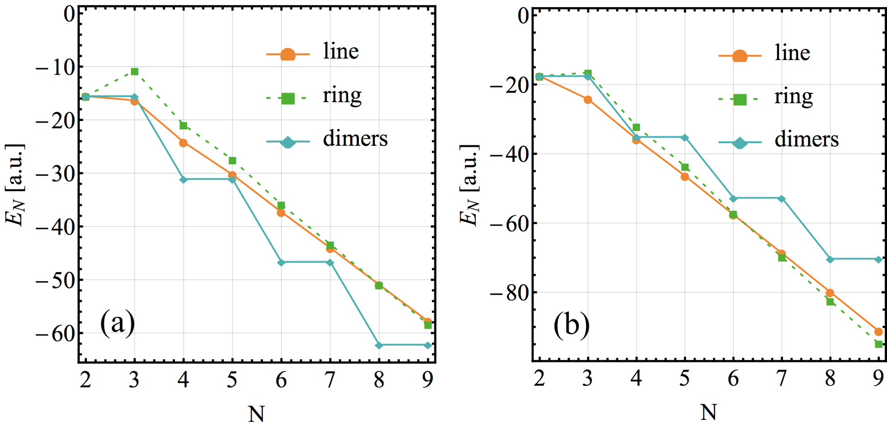
Figure 4: The lowest energy for on-the-line and on-the-ring configurations for $\Delta_{d}/\nu_{c}$ $=$ $0.4$ for (a) Rb and (b) Cs. We see that strong N-body forces lead to different geometry of the ground state depending on $N$ and the atomic species.

From Fig. 4(a), we see that the few-body forces lead to an effect in which many photons prefer to be arranged as independent dimers. For Cs [see Fig. 4(b)] at large enough $N$ (which depends on $\Delta_{d}/\nu_{q}$, and for $\Delta_{d}/\nu_{q}$ $=$ $0.4$ happens for $N\geq 7$), a regular polygon (ring) is the ground state rather than a linear configuration [see Fig. 1(d)]. Intuitively, the additional two-body attractive bond for the ring arrangement wins over the additional repulsive many-body forces present in this configuration.

Experimental realization

Photons in a multi-mode cavity Sommer2015 enable us to tune the polariton’s mass so that $mV_{e}$ is repulsive at short distances, has local minima at finite distance, and is free of potentially lossy divergences Maghrebi2015c ; Bienias2014 ; Gullans2017 . In general, for multi-mode cavities, the generation of the mass is intertwined with the presence of the trapping potential. However, for a near-planar cavity (defined as $R\gg L$, where $R$ is mirror curvature and $L$ distance between mirrors) we have $m_{\rm\scriptscriptstyle ph}$ $=$ $\frac{k}{c}$ and the trapping frequency $\omega_{\rm\scriptscriptstyle tr}$ $=$ $\frac{c}{\sqrt{2LR}}$. Therefore, the trapping vanishes with increasing $LR$.

Note that our scheme also works in a free-space quasi-1D geometry Peyronel2012 for a magnetic field perpendicular to the propagation direction and the transverse mass much greater than the longitudinal one Gullans2017 . Then, by working in the regime $\Omega>|\Delta|$, we can achieve a divergence-free potential that is repulsive at short distances Maghrebi2015c ; Bienias2014 .

To prepare the ground state on small systems we envision a spectroscopic post-selection approach whereby a weak product coherent state wavefunction is input with the mode frequencies chosen to add up to the energy of the target ground state. The mode functions of the photons can be further chosen to maximize the ground-state overlap. State preparation is then possible through post-selection on the total photon number. The weak input condition ensures that the target manifold is not spoiled by dissipation from higher-photon number manifolds. For larger systems, more efficient preparation schemes become necessary that are still insensitive to dissipation. We imagine using dissipative Rydberg blockade Peyronel2012 ; Dudin2012 to prepare a product state of many single photons as the starting state for adiabatic transfer to the ground state. This method is robust to dissipation for ground state gaps larger than the dissipation rate. Once the state is prepared, the measured multi-body 2D correlation functions can be postprocessed Schauss2012 to prevent the rotational symmetry and shot-to-shot variations in measurement outcomes from smearing out spatial patterns. We leave a more complete and detailed analysis of preparation and detection for future work.

Outlook

In this work, we concentrated on the strongly interacting regime in 1D and 2D. Another direction is a study of the 3D interacting regime of photons copropagating in free space in the presence of the molecular potential in the transverse directions Sevincli2011 ; Gullans2017 . Note that our analysis suggests that the strong few-body forces can also be observed in experiments with ultracold Rydberg atoms alone Schauss2012b ; Zeiher2017 rather than Rydberg-polaritons. This can be done in a 2D pancake geometry with or without an additional optical lattice potential. It is an especially promising direction in the light of recent work on the observation of Rydberg macrodimers Hollerith2019 with $P$ states close to Förster resonances.

Supplemental material

Here, we present the derivation of effective interactions between polaritons propagating through Rydberg media close to the Förster resonance (sec. I), derivation of the characteristic energy and length scales in the two-body problem (sec. II), derivation of the single-channel description used to give intuition behind three-body forces (sec. III), and self-consistent solution of the four body problem (sec. IV).

I Two photons propagating through Rydberg media close to the Förster resonance

Here, we give more details related to the effective interactions between Rydberg states described by Eq. (9) in the main text. Our model system is a one-dimensional gas of atoms whose electronic levels are given in Fig. 1(a) in the main text. Following Ref. Gorshkov2011 ; Peyronel2012 ; Bienias2014 ; Gorniaczyk2016 , we introduce operators $\hat{I}^{\dagger}(z)$ and $\hat{S}^{\dagger}(z)$ which generate the atomic excitations into the $\left|I\right\rangle$ and $\left|S\right\rangle$ states, respectively, at position $z$. In addition, comparing to Ref. Gorshkov2011 ; Peyronel2012 ; Bienias2014 ; Bienias2016a ; Gorniaczyk2016 we include a more complex atomic level structure of the source and the gate excitations by defining $\hat{{P}}_{1}^{\dagger}(z)$ and $\hat{{P}}_{2}^{\dagger}(z)$ which create excitations into $\left|P_{1}\right\rangle$ and $\left|P_{2}\right\rangle$ states, respectively. All the operators $\hat{O}(z)\in\{\hat{\mathcal{E}}(z)\,,\hat{I}(z)\,,\hat{S}(z)\,,\hat{{P}_{1}}(z)\,,\hat{{P}_{2}}(z)$ are bosonic and satisfy the equal time commutation relation, $[\hat{O}(z),\hat{O}^{\dagger}(z^{\prime})]=\delta(z-z^{\prime})$.

The microscopic Hamiltonian describing the propagation consists of three parts: $\hat{H}=\hat{H}_{\text{p}}+\hat{H}_{\text{ap}}+\hat{H}_{\text{int}}$. For the sake of simplicity we show the derivation for the 1D massive photons, which straightforwardly applies to the free-space photons within the center of mass frame, and generalizes to a 2D cavity. The first term describes the photon evolution in the medium and is defined as

$$\hat{H}_{\text{p}}=-\frac{1}{2m_{\rm\scriptscriptstyle ph}}\int dz\hat{\mathcal{E}}^{\dagger}(z)\partial^{2}_{z}\hat{\mathcal{E}}(z),$$ (14)

with the mass defined by the cavity geometry. The atom-photon coupling is described by

$$\hat{H}_{\text{ap}}=\int dz \bigg{[} g\hat{\mathcal{E}}(z)\hat{I}^{\dagger}(z)+\Omega\hat{S}^{\dagger}(z)\hat{I}(z)+g\hat{{I}}(z)\hat{\mathcal{E}}^{\dagger}(z)+\Omega\hat{I}^{\dagger}(z)\hat{S}(z)+{\Delta}{}\hat{I}^{\dagger}(z)\hat{I}(z)\bigg{]},$$ (15)

where $g$ is the collective coupling of the photons to the matter, and for the sake of brevity we drop the decay rates $\gamma_{S}$, $\gamma_{P_{1}}$ and $\gamma_{P_{2}}$. The interaction between Rydberg levels is described by

$$\hat{H}_{\text{int}}=\frac{1}{2}\int dz^{\prime}\int dz\begin{pmatrix}\hat{S}\hat{S}\\ \hat{P_{1}}\hat{P_{2}}\\ \hat{P_{2}}\hat{P_{1}}\end{pmatrix}^{\dagger}\!\left(\begin{array}[]{ccc}V_{SS}&V_{d}&V_{d}\\ V^{*}_{d}&V_{PP}+\Delta_{d}&V_{PP,\text{off}}\\ V^{*}_{d}&V_{PP,\text{off}}&V_{PP}+\Delta_{d}\\ \end{array}\right)\begin{pmatrix}\hat{S}\hat{S}\\ \hat{P_{1}}\hat{P_{2}}\\ \hat{P_{2}}\hat{P_{1}}\end{pmatrix},$$ (19)

where the notation was explained in the main text. The Schroedinger equation has the form

$$i\hbar\partial_{t}\left|\psi(t)\right\rangle=\hat{H}\left|\psi(t)\right\rangle,$$ (20)

with the two-excitation wavefunction having the form Peyronel2012 ; Bienias2016a

$$\left|\psi(t)\right\rangle = \int\!\mathrm{d}z\,\int\!\mathrm{d}z^{\prime}\,{\bigg{[}}\left.\frac{1}{2}{\mathcal{E}\mathcal{E}}(z,z^{\prime},t)\hat{\mathcal{E}}^{\dagger}(z)\hat{\mathcal{E}^{\dagger}}(z^{\prime})+\frac{1}{2}{PP}(z,z^{\prime},t)\hat{P}^{\dagger}(z)\hat{P^{\dagger}}(z^{\prime})+\frac{1}{2}{SS}(z,z^{\prime},t)\hat{S}^{\dagger}(z)\hat{S^{\dagger}}(z^{\prime})\right.$$

$$+ \left.{{\mathcal{E}}P}(z,z^{\prime},t)\hat{\mathcal{E}}^{\dagger}(z)\hat{P^{\dagger}}(z^{\prime})+{\mathcal{E}S}(z,z^{\prime},t)\hat{\mathcal{E}}^{\dagger}(z)\hat{S^{\dagger}}(z^{\prime})+{PS}(z,z^{\prime},t)\hat{P}^{\dagger}(z)\hat{S^{\dagger}}(z^{\prime})+{P_{1}P_{2}}(z,z^{\prime},t)\hat{P}^{\dagger}_{1}(z)\hat{P_{2}^{\dagger}}(z^{\prime})\right.{\bigg{]}}\left|0\right\rangle.$$

The Schroedinger equation Peyronel2012 in the frequency space reduces to

$$\omega\mathcal{E}\mathcal{E}(z,z^{\prime}) =-\frac{1}{2m_{\rm\scriptscriptstyle ph}}\left(\partial^{2}_{z}+\partial^{2}_{z^{\prime}}\right)\mathcal{E}\mathcal{E}(z,z^{\prime})+g(\mathcal{E}{I}(z,z^{\prime})+\mathcal{E}{I}(z^{\prime},z)),$$ (22)

$$\omega\mathcal{E}{I}(z,z^{\prime}) =\left(-\frac{1}{2m_{\rm\scriptscriptstyle ph}}\partial^{2}_{z}+\Delta\right)\mathcal{E}{I}(z,z^{\prime})+g{I}{I}(z,z^{\prime})+\Omega\mathcal{E}S(z,z^{\prime}),$$ (23)

$$\omega\mathcal{E}S(z,z^{\prime}) =\left(-\frac{1}{2m_{\rm\scriptscriptstyle ph}}\partial^{2}_{z}+\Delta\right)\mathcal{E}S(z,z^{\prime})+g{I}S(z,z^{\prime})+\Omega\mathcal{E}{I}(z,z^{\prime}),$$ (24)

$$\omega{I}{I}(z,z^{\prime}) =2\Delta{I}{I}(z,z^{\prime})+g(\mathcal{E}{I}(z,z^{\prime})+\mathcal{E}{I}(z^{\prime},z))+\Omega({I}S(z,z^{\prime})+{I}S(z^{\prime},z)),$$ (25)

$$\omega{I}S(z,z^{\prime}) =\Delta{I}S(z,z^{\prime})+g\mathcal{E}S(z,z^{\prime})+\Omega SS(z,z^{\prime}),$$ (26)

$$\omega SS(z,z^{\prime}) =\Omega({I}S(z,z^{\prime})+{I}S(z^{\prime},z))+V_{SS}(z-z^{\prime})SS(z,z^{\prime})+V_{d}(z-z^{\prime})\left({P}_{1}{P}_{2}(z,z^{\prime})+{P}_{1}{P}_{2}(z^{\prime},z)\right),$$ (27)

$$\omega{P}_{1}{P}_{2}(z,z^{\prime}) =V^{*}_{d}(z-z^{\prime})SS(z,z^{\prime})+V_{PP}(z-z^{\prime}){P}_{1}{P}_{2}(z,z^{\prime})+\Delta_{d}{P}_{1}{P}_{2}(z,z^{\prime})+V_{PP,{\rm\scriptscriptstyle off}}(z-z^{\prime}){P}_{1}{P}_{2}(z^{\prime},z),$$ (28)

where only the two last equations differ from the conventional one Gorshkov2011 ; Peyronel2012 ; Bienias2014 ; Gorniaczyk2016 .

Next, we eliminate the ${P}_{1}{P}_{2}$ component

$${P}_{1}{P}_{2}(z,z^{\prime}) =\frac{V^{*}_{d}(z-z^{\prime})}{\omega-V_{PP}(z-z^{\prime})-\Delta_{d}-V_{PP,{\rm\scriptscriptstyle off}}(z-z^{\prime})}SS(z,z^{\prime}),$$ (29)

which is not coupled by the laser field directly to photons. This leads to

$$\omega SS(z,z^{\prime}) =\left(V_{SS}(z-z^{\prime})-\frac{2V_{d}(z-z^{\prime})^{2}}{\Delta_{d}+V_{PP}(z-z^{\prime})+V_{PP,{\rm\scriptscriptstyle off}}(z-z^{\prime})-\omega}\right)SS(z,z^{\prime})+\Omega({I}S(z,z^{\prime})+{I}S(z^{\prime},z)).$$ (30)

Note that $S(z,z^{\prime})=S(z^{\prime},z)$. We see from Eq. (30) that the effective interaction between Rydberg states takes the form shown in Eq. (3) in the main text.

II The characteristic energy and lengths scales in the two body problem

Let us next comment in more detail on the form of the $V_{f}(r)$ given by Eq. (9) in the main text. Since $|V_{f}|\ll\omega_{c}$, the depth of $V_{e}$ is nearly equal to the depth of $V_{f}$ in the considered regime, and is given by $V_{\rm\scriptscriptstyle min}=-{(\sqrt{2}C_{3}-\sqrt{C_{SS}\left(\Delta_{d}-\omega\right)})^{2}}/{C_{PP}}$; note that we consider states for which $C_{PP},C_{SS}$>0. The minimum of the potential occurs at the relative distance given by $r^{6}={C_{PP}\sqrt{C_{SS}}}/$$\left({\sqrt{2}C_{3}\sqrt{\Delta_{d}-\omega}-\sqrt{C_{SS}}(\Delta_{d}-\omega)}\right),$ which leads to a characteristic length scale $b=\left({\left(\sqrt{2}+1\right)C_{PP}C_{SS}}/{C_{3}^{2}}\right)^{1/6}$, by taking $\Delta_{d}=\nu_{c}/2$ with $\nu_{c}=2C_{3}^{2}/C_{SS}$. The potential’s local minimum exists for $C_{SS}\left(\omega-\Delta_{d}\right)+2C_{3}^{2}>0$. For $\omega=0$ and $\epsilon=\Delta_{d}/\nu_{c}<1$ we have $V_{\rm\scriptscriptstyle min}=-{2C_{3}^{2}\left(\sqrt{\epsilon}-1\right)^{2}}/{C_{PP}}$. Therefore, we define $V_{c}={2C_{3}^{2}}/{C_{PP}}$, which together with $\nu_{c}$ is used as a characteristic energy scale in our results.

III Comparison of single-channel $PP$ vs double-channel $P_{1}P_{2}$ physics

We illustrate the relation between the effective $PP$ channel description (i.e., Eq. (12) in the main text) and the two channels $P_{1}P_{2}$ and $P_{2}P_{1}$ description for the three-body problem. For the sake of simplicity we neglect weaker off-diagonal vdW interactions $V_{PP,{\rm\scriptscriptstyle off}}$.

We consider the Hamiltonian in the following basis: $\left|SSS\right\rangle$, $\left|SP_{1}P_{2}\right\rangle$, $\left|SP_{2}P_{1}\right\rangle$, $\left|P_{1}SP_{2}\right\rangle$,$\left|P_{1}P_{2}S\right\rangle$, $\left|P_{2}SP_{1}\right\rangle$, and $\left|P_{2}P_{1}S\right\rangle$. The off-diagonal part of the Hamiltonian:

$$\vspace{-0em}\left(\begin{array}[]{ccccccc}0&\frac{e^{2i\phi_{2,3}}C_{d}}{r_{2,3}^{3}}&\frac{e^{2i\phi_{2,3}}C_{d}}{r_{2,3}^{3}}&\frac{e^{2i\phi_{1,3}}C_{d}}{r_{1,3}^{3}}&\frac{e^{2i\phi_{1,2}}C_{d}}{r_{1,2}^{3}}&\frac{e^{2i\phi_{1,3}}C_{d}}{r_{1,3}^{3}}&\frac{e^{2i\phi_{1,2}}C_{d}}{r_{1,2}^{3}}\\ \frac{e^{-2i\phi_{2,3}}C_{d}}{r_{2,3}^{3}}&0&0&\frac{C_{d,1}}{r_{1,2}^{3}}&0&0&\frac{C_{d,2}}{r_{1,3}^{3}}\\ \frac{e^{-2i\phi_{2,3}}C_{d}}{r_{2,3}^{3}}&0&0&0&\frac{C_{d,1}}{r_{1,3}^{3}}&\frac{C_{d,2}}{r_{1,2}^{3}}&0\\ \frac{e^{-2i\phi_{1,3}}C_{d}}{r_{1,3}^{3}}&\frac{C_{d,1}}{r_{1,2}^{3}}&0&0&\frac{C_{d,2}}{r_{2,3}^{3}}&0&0\\ \frac{e^{-2i\phi_{1,2}}C_{d}}{r_{1,2}^{3}}&0&\frac{C_{d,1}}{r_{1,3}^{3}}&\frac{C_{d,2}}{r_{2,3}^{3}}&0&0&0\\ \frac{e^{-2i\phi_{1,3}}C_{d}}{r_{1,3}^{3}}&0&\frac{C_{d,2}}{r_{1,2}^{3}}&0&0&0&\frac{C_{d,1}}{r_{2,3}^{3}}\\ \frac{e^{-2i\phi_{1,2}}C_{d}}{r_{1,2}^{3}}&\frac{C_{d,2}}{r_{1,3}^{3}}&0&0&0&\frac{C_{d,1}}{r_{2,3}^{3}}&0\\ \end{array}\right),\vspace{-0.em}$$ (31)

whereas the diagonal one

$$\vspace{-0em}\left(\begin{array}[]{c}\frac{C_{\text{SS}}}{r_{1,2}^{6}}+\frac{C_{\text{SS}}}{r_{1,3}^{6}}+\frac{C_{\text{SS}}}{r_{2,3}^{6}}\\ \frac{C_{P_{1}P_{2}}}{r_{2,3}^{6}}+\Delta_{d}+\frac{C_{\text{SP}_{1}}}{r_{1,2}^{6}}+\frac{C_{\text{SP}_{2}}}{r_{1,3}^{6}}\\ \frac{C_{P_{1}P_{2}}}{r_{2,3}^{6}}+\Delta_{d}+\frac{C_{\text{SP}_{2}}}{r_{1,2}^{6}}+\frac{C_{\text{SP}_{1}}}{r_{1,3}^{6}}\\ \frac{C_{P_{1}P_{2}}}{r_{1,3}^{6}}+\Delta_{d}+\frac{C_{\text{SP}_{1}}}{r_{1,2}^{6}}+\frac{C_{\text{SP}_{2}}}{r_{2,3}^{6}}\\ \frac{C_{P_{1}P_{2}}}{r_{1,2}^{6}}+\Delta_{d}+\frac{C_{\text{SP}_{1}}}{r_{1,3}^{6}}+\frac{C_{\text{SP}_{2}}}{r_{2,3}^{6}}\\ \frac{C_{P_{1}P_{2}}}{r_{1,3}^{6}}+\Delta_{d}+\frac{C_{\text{SP}_{2}}}{r_{1,2}^{6}}+\frac{C_{\text{SP}_{1}}}{r_{2,3}^{6}}\\ \frac{C_{P_{1}P_{2}}}{r_{1,2}^{6}}+\Delta_{d}+\frac{C_{\text{SP}_{2}}}{r_{1,3}^{6}}+\frac{C_{\text{SP}_{1}}}{r_{2,3}^{6}}\\ \end{array}\right),\vspace{-0.em}$$ (32)

where $C_{d}$ denotes dipolar interactions between $SS$ and $P_{1}P_{2}$, $C_{d,1}$ between $SP_{1}$ and $P_{1}S$, and $C_{d,2}$ between $SP_{2}$ and $P_{2}S$. Terms without index _d denote vdW interactions.

In order to present the following argument, it is enough to consider only the Hamiltonian elements between five states (out of seven) which we do for the clarity of presentation: We rotate the interaction Hamiltonian into the symmetric and asymmetric basis $\left|SSS\right\rangle,\frac{1}{\sqrt{2}}(\left|SP_{1}P_{2}\right\rangle\pm\left|SP_{2}P_{1}\right\rangle)$, and $\frac{1}{\sqrt{2}}(\left|P_{1}SP_{2}\right\rangle\pm\left|P_{2}SP_{1}\right\rangle)$. The off-diagonal terms are:

$$\vspace{-0em}\left(\begin{array}[]{ccccc}0&\frac{\sqrt{2}e^{2i\phi_{2,3}}C_{d}}{r_{2,3}^{3}}&0&\frac{\sqrt{2}e^{2i\phi_{1,3}}C_{d}}{r_{1,3}^{3}}&0\\ \frac{\sqrt{2}e^{-2i\phi_{2,3}}C_{d}}{r_{2,3}^{3}}&0&\frac{\left(C_{\text{SP}_{2}}-C_{\text{SP}_{1}}\right)\left(r_{1,2}^{6}-r_{1,3}^{6}\right)}{2r_{1,2}^{6}r_{1,3}^{6}}&\frac{C_{d,1}+C_{d,2}}{2r_{1,2}^{3}}&\frac{C_{d,1}-C_{d,2}}{2r_{1,2}^{3}}\\ 0&\frac{\left(C_{\text{SP}_{2}}-C_{\text{SP}_{1}}\right)\left(r_{1,2}^{6}-r_{1,3}^{6}\right)}{2r_{1,2}^{6}r_{1,3}^{6}}&0&\frac{C_{d,1}-C_{d,2}}{2r_{1,2}^{3}}&\frac{C_{d,1}+C_{d,2}}{2r_{1,2}^{3}}\\ \frac{\sqrt{2}e^{-2i\phi_{1,3}}C_{d}}{r_{1,3}^{3}}&\frac{C_{d,1}+C_{d,2}}{2r_{1,2}^{3}}&\frac{C_{d,1}-C_{d,2}}{2r_{1,2}^{3}}&0&\frac{\left(C_{\text{SP}_{2}}-C_{\text{SP}_{1}}\right)\left(r_{1,2}^{6}-r_{2,3}^{6}\right)}{2r_{1,2}^{6}r_{2,3}^{6}}\\ 0&\frac{C_{d,1}-C_{d,2}}{2r_{1,2}^{3}}&\frac{C_{d,1}+C_{d,2}}{2r_{1,2}^{3}}&\frac{\left(C_{\text{SP}_{2}}-C_{\text{SP}_{1}}\right)\left(r_{1,2}^{6}-r_{2,3}^{6}\right)}{2r_{1,2}^{6}r_{2,3}^{6}}&0\\ \end{array}\right),\vspace{-0.em}$$ (33)

whereas the diagonal one:

$$\vspace{-0em}\left(\begin{array}[]{c}C_{\text{SS}}\left(\frac{1}{r_{1,3}^{6}}+\frac{1}{r_{2,3}^{6}}+\frac{1}{r_{1,2}^{6}}\right)\\ \frac{C_{P_{1}P_{2}}}{r_{2,3}^{6}}+\Delta_{d}+\frac{1}{2}C_{\text{SP}_{1}}\left(\frac{1}{r_{1,3}^{6}}+\frac{1}{r_{1,2}^{6}}\right)+\frac{1}{2}C_{\text{SP}_{2}}\left(\frac{1}{r_{1,3}^{6}}+\frac{1}{r_{1,2}^{6}}\right)\\ \frac{C_{P_{1}P_{2}}}{r_{2,3}^{6}}+\Delta_{d}+\frac{1}{2}C_{\text{SP}_{1}}\left(\frac{1}{r_{1,3}^{6}}+\frac{1}{r_{1,2}^{6}}\right)+\frac{1}{2}C_{\text{SP}_{2}}\left(\frac{1}{r_{1,3}^{6}}+\frac{1}{r_{1,2}^{6}}\right)\\ \frac{C_{P_{1}P_{2}}}{r_{1,3}^{6}}+\Delta_{d}+\frac{1}{2}C_{\text{SP}_{1}}\left(\frac{1}{r_{2,3}^{6}}+\frac{1}{r_{1,2}^{6}}\right)+\frac{1}{2}C_{\text{SP}_{2}}\left(\frac{1}{r_{2,3}^{6}}+\frac{1}{r_{1,2}^{6}}\right)\\ \frac{C_{P_{1}P_{2}}}{r_{1,3}^{6}}+\Delta_{d}+\frac{1}{2}C_{\text{SP}_{1}}\left(\frac{1}{r_{2,3}^{6}}+\frac{1}{r_{1,2}^{6}}\right)+\frac{1}{2}C_{\text{SP}_{2}}\left(\frac{1}{r_{2,3}^{6}}+\frac{1}{r_{1,2}^{6}}\right)\\ \end{array}\right).\vspace{-0.em}$$ (34)

From the off-diagonal terms we see the $\sqrt{2}$ enhancement of the coupling from $SS$ to the symmetric-superposition channel denoted by the $PP$ in the main text. Coefficients $C_{PP},C_{SP}$ in the main text correspond to the averages of corresponding two-channel quantities.

We see that for the generic geometry with $r_{ij}\neq r_{jk}$, decoupling from asymmetric channels requires $C_{SP_{1}}\approx C_{SP_{2}}$ and $C_{d,1}\approx C_{d,2}$. In our proposal we use $n_{1}=n$ and $n_{2}=n-1$ with $n=120\gg 1$ for which $C_{SP_{1}}/C_{SP_{2}}\approx 0.98$ $C_{d,1}/C_{d_{2}}\approx 0.92$. This enables us to use the effective single-channel picture to give an intuition behind the multi-body forces. Note that all the numerical results presented in the main text are performed without the single-channel approximation. Finally, the single-channel picture is valid only for two- and three-body problem.

IV Four-body problem

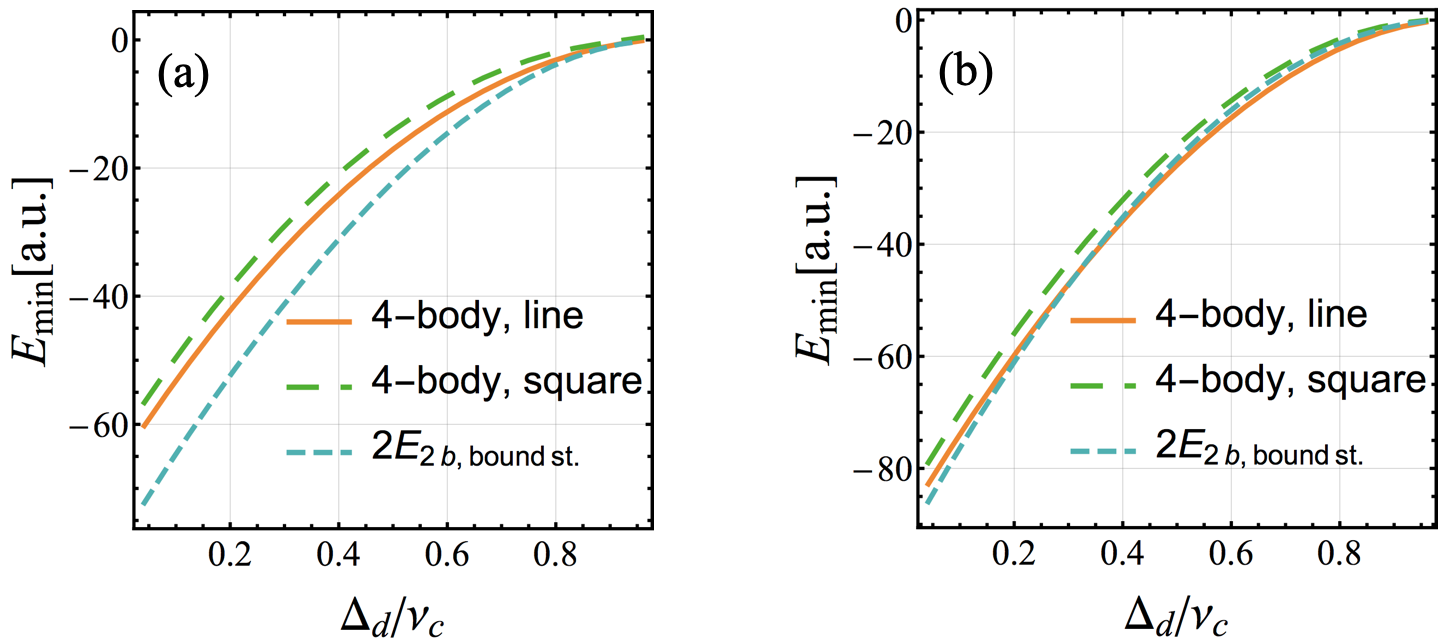
Figure 5: Self-consistent solution of Eq. (6) in the main text describing polaritons in the large-mass limit. (a-b) Lowest energy as a function of $\Delta_{d}$ for line, regular-polygon, and dimer configurations for four bodies. Results are shown in (a) for ⁸⁷Rb and in (b) for ¹³³Cs; all of them are for $n_{1},n_{2},n$ as in Fig. 2 in the main text.

The four-body problem features additional exotic phenomena due to the strong four-body interactions. For ⁸⁷Rb, the ground state is a configuration consisting of two far-separated dimers foot8 , see Fig. 5(a). However for ¹³³Cs, which has $C_{SP}/C_{PP}$ $\approx$ $0.6$ (compared with $C_{SP}/C_{PP}$ $\approx$ $1.4$ for ⁸⁷Rb) and therefore weaker multi-body forces, the ground state configuration depends on $\Delta_{d}$, Fig. 5(b): the ground state is a linear configuration for $\Delta_{d}/\nu_{c}\geq 0.3$ and two far-separated dimers for $\Delta_{d}/\nu_{c}\leq 0.3$ foot9 .

References

- (1) I. Bloch, W. Zwerger and J. Dalibard, Many-body physics with ultracold gases, Rev. Mod. Phys., 80, 885–964 (2008).
- (2) C. Chin, R. Grimm, P. Julienne and E. Tiesinga, Feshbach resonances in ultracold gases, Rev. Mod. Phys., 82, 1225–1286 (2010).
- (3) R. M. W. van Bijnen and T. Pohl, Quantum Magnetism and Topological Ordering via Rydberg Dressing near Förster Resonances, Phys. Rev. Lett., 114, 243002 (2015).
- (4) A. W. Glaetzle, M. Dalmonte, R. Nath, C. Gross, I. Bloch and P. Zoller, Designing frustrated quantum magnets with laser-dressed Rydberg atoms, Phys. Rev. Lett., 114, 173002 (2015).
- (5) T. Grass, P. Bienias, M. J. Gullans, R. Lundgren, J. Maciejko and A. V. Gorshkov, Fractional Quantum Hall Phases of Bosons with Tunable Interactions: From the Laughlin Liquid to a Fractional Wigner Crystal, Phys. Rev. Lett., 121, 253403 (2018).
- (6) D. E. Chang, V. Vuletić and M. D. Lukin, Quantum nonlinear optics - Photon by photon, Nat. Photonics, 8, 685–694 (2014).
- (7) T. Caneva, M. T. Manzoni, T. Shi, J. S. Douglas, J. I. Cirac and D. E. Chang, Quantum dynamics of propagating photons with strong interactions: a generalized input-output formalism, New J. Phys., 17, 113001 (2015).
- (8) M. Fleischhauer and M. D. Lukin, Dark-state polaritons in electromagnetically induced transparency, Phys. Rev. Lett., 84, 5094–5097 (2000).
- (9) M. D. Lukin, M. Fleischhauer, R. Cote, L. M. Duan, D. Jaksch, J. I. Cirac and P. Zoller, Dipole blockade and quantum information processing in mesoscopic atomic ensembles, Phys. Rev. Lett., 87, 037901 (2001).
- (10) I. Friedler, D. Petrosyan, M. Fleischhauer and G. Kurizki, Long-range interactions and entanglement of slow single-photon pulses, Phys. Rev. A, 72, 043803 (2005).
- (11) J. D. Pritchard, D. Maxwell, A. Gauguet, K. J. Weatherill, M. P. A. Jones and C. S. Adams, Cooperative atom-light interaction in a blockaded Rydberg ensemble, Phys. Rev. Lett., 105, 193603 (2010).
- (12) O. Firstenberg, T. Peyronel, Q. Y. Liang, A. V. Gorshkov, M. D. Lukin and V. Vuletić, Attractive photons in a quantum nonlinear medium, Nature, 502, 71–75 (2013).
- (13) P. Bienias, S. Choi, O. Firstenberg, M. F. Maghrebi, M. Gullans, M. D. Lukin, A. V. Gorshkov and H. P. Büchler, Scattering resonances and bound states for strongly interacting Rydberg polaritons, Phys. Rev. A, 90, 053804 (2014).
- (14) P. Bienias, Few-body quantum physics with strongly interacting Rydberg polaritons, Eur. Phys. J. Spec. Top., 225, 2957–2976 (2016).
- (15) P. Bienias and H. P. Büchler, Two photon conditional phase gate based on Rydberg slow light polaritons, J. Phys. B At. Mol. Opt. Phys., 53, 54003 (2020).
- (16) D. Tiarks, S. Schmidt-Eberle, T. Stolz, G. Rempe and S. Dürr, A photon–photon quantum gate based on Rydberg interactions, Nat. Phys., 15, 124–126 (2019).
- (17) D. Tiarks, S. Schmidt, G. Rempe and S. Dürr, Optical phase shift created with a single-photon pulse, Sci. Adv., 2, e1600036–e1600036 (2016).
- (18) D. Tiarks, S. Baur, K. Schneider, S. Dürr and G. Rempe, Single-photon transistor using a Förster resonance, Phys. Rev. Lett., 113, 053602 (2014).
- (19) H. Gorniaczyk, C. Tresp, J. Schmidt, H. Fedder and S. Hofferberth, Single-photon transistor mediated by interstate Rydberg interactions, Phys. Rev. Lett., 113, 053601 (2014).
- (20) H. Gorniaczyk, C. Tresp, P. Bienias, A. Paris-Mandoki, W. Li, I. Mirgorodskiy, H. P. Büchler, I. Lesanovsky and S. Hofferberth, Enhancement of Rydberg-mediated single-photon nonlinearities by electrically tuned Förster resonances, Nat. Commun., 7, 12480 (2016).
- (21) Y. O. Dudin and A. Kuzmich, Strongly interacting Rydberg excitations of a cold atomic gas, Science, 336, 887–889 (2012).
- (22) T. Peyronel, O. Firstenberg, Q. Y. Liang, S. Hofferberth, A. V. Gorshkov, T. Pohl, M. D. Lukin and V. Vuletić, Quantum nonlinear optics with single photons enabled by strongly interacting atoms, Nature, 488, 57–60 (2012).
- (23) D. Ornelas Huerta, A. Craddock, E. Goldschmidt, A. Hachtel, Y. Wang, P. Bienias, A. Gorshkov, S. Rolston and J. Porto, On-demand indistinguishable single photons from an efficient and pure source based on a Rydberg ensemble, Optica, 7, 813 (2020).
- (24) P. Bienias, J. Douglas, A. Paris-Mandoki, P. Titum, I. Mirgorodskiy, C. Tresp, E. Zeuthen, M. J. Gullans, M. Manzoni, S. Hofferberth, D. Chang and A. V. Gorshkov, Photon propagation through dissipative Rydberg media at large input rates, Phys. Rev. Res., 2, 033049 (2020).
- (25) These bound states Maghrebi2015c are based on the singular potentials that lead to significant losses for experimentally relevant parameters.
- (26) J. S. Douglas, T. Caneva and D. E. Chang, Photon molecules in atomic gases trapped near photonic crystal waveguides, Phys. Rev. X, 6, 031017 (2016).
- (27) M. F. Maghrebi, M. J. Gullans, P. Bienias, S. Choi, I. Martin, O. Firstenberg, M. D. Lukin, H. P. Büchler and A. V. Gorshkov, Coulomb Bound States of Strongly Interacting Photons, Phys. Rev. Lett., 115, 123601 (2015).
- (28) K. Afrousheh, P. Bohlouli-Zanjani, D. Vagale, A. Mugford, M. Fedorov and J. D. Martin, Spectroscopic observation of resonant electric dipole-dipole interactions between cold Rydberg atoms, Phys. Rev. Lett., 93, 233001 (2004).
- (29) P. Bohlouli-Zanjani, J. A. Petrus and J. D. Martin, Enhancement of rydberg atom interactions using ac stark shifts, Phys. Rev. Lett., 98, 203005 (2007).
- (30) T. Vogt, M. Viteau, J. Zhao, A. Chotia, D. Comparat and P. Pillet, Dipole blockade at förster resonances in high resolution laser excitation of rydberg states of cesium atoms, Phys. Rev. Lett., 97, 083003 (2006).
- (31) I. I. Ryabtsev, D. B. Tretyakov, I. I. Beterov and V. M. Entin, Observation of the stark-tuned förster resonance between two rydberg atoms, Phys. Rev. Lett., 104, 073003 (2010).
- (32) A. Reinhard, K. C. Younge, T. C. Liebisch, B. Knuffman, P. R. Berman and G. Raithel, Double-resonance spectroscopy of interacting Rydberg-atom systems, Phys. Rev. Lett., 100, 233201 (2008).
- (33) J. Nipper, J. B. Balewski, A. T. Krupp, S. Hofferberth, R. Löw and T. Pfau, Atomic pair-state interferometer: Controlling and measuring an interaction-induced phase shift in rydberg-atom pairs, Phys. Rev. X, 2, 031011 (2012).
- (34) S. Ravets, H. Labuhn, D. Barredo, T. Lahaye and A. Browaeys, Measurement of the angular dependence of the dipole-dipole interaction between two individual Rydberg atoms at a Förster resonance, Phys. Rev. A, 92, 020701(R) (2015).
- (35) B. Pelle, R. Faoro, J. Billy, E. Arimondo, P. Pillet and P. Cheinet, Quasiforbidden two-body Förster resonances in a cold Cs Rydberg gas, Phys. Rev. A, 93, 023417 (2016).
- (36) I. I. Beterov and M. Saffman, Rydberg blockade, Förster resonances, and quantum state measurements with different atomic species, Phys. Rev. A, 92, 042710 (2015).
- (37) G. Günter, M. Robert-de Saint-Vincent, H. Schempp, C. S. Hofmann, S. Whitlock and M. Weidemüller, Interaction enhanced imaging of individual Rydberg atoms in dense gases, Phys. Rev. Lett., 108, 013002 (2012).
- (38) B. Olmos, W. Li, S. Hofferberth and I. Lesanovsky, Amplifying single impurities immersed in a gas of ultracold atoms, Phys. Rev. A, 84, 041607(R) (2011).
- (39) G. Guenter, H. Schempp, M. Robert-de Saint-Vincent, V. Gavryusev, S. Helmrich, C. S. Hofmann, S. Whitlock and M. Weidemueller, Observing the dynamics of dipole-mediated energy transport by interaction-enhanced imaging, Science, 342, 954–956 (2013).
- (40) J. Otterbach, M. Moos, D. Muth and M. Fleischhauer, Wigner crystallization of single photons in cold rydberg ensembles, Phys. Rev. Lett., 111, 113001 (2013).
- (41) D. E. Chang, V. Gritsev, G. Morigi, V. Vuletić, M. D. Lukin and E. A. Demler, Crystallization of strongly interacting photons in a nonlinear optical fibre, Nat. Phys., 4, 884–889 (2008).
- (42) A. Sommer, H. P. Büchler and J. Simon, Quantum Crystals and Laughlin Droplets of Cavity Rydberg Polaritons, ArXiv:1506.00341 (2015).
- (43) K. Jachymski, P. Bienias and H. P. Büchler, Three-body interactions of slow light Rydberg polaritons, Phys. Rev. Lett., 117, 053601 (2016).
- (44) M. J. Gullans, J. D. Thompson, Y. Wang, Q. Y. Liang, V. Vuletić, M. D. Lukin and A. V. Gorshkov, Effective Field Theory for Rydberg Polaritons, Phys. Rev. Lett., 117, 113601 (2016).
- (45) M. Kalinowski, Y. Wang, P. Bienias, M. J. Gullans, D. Ornelas-Huerta, A. N. Craddock, S. Rolston, H. P. Buechler and A. V. Gorshkov, Enhancement and tunability of three-body loss between strongly interacting photons, In prep (2020).
- (46) Q.-Y. Liang, A. V. Venkatramani, S. H. Cantu, T. L. Nicholson, M. J. Gullans, A. V. Gorshkov, J. D. Thompson, C. Chin, M. D. Lukin and V. Vuletić, Observation of three-photon bound states in a quantum nonlinear medium, Science, 359, 783–786 (2018).
- (47) A. Sommer and J. Simon, Engineering photonic Floquet Hamiltonians through Fabry-Pérot resonators, New J. Phys., 18, 35008 (2016).
- (48) N. Schine, A. Ryou, A. Gromov, A. Sommer and J. Simon, Synthetic Landau levels for photons, Nature, 534, 671 (2016).
- (49) N. Jia, N. Schine, A. Georgakopoulos, A. Ryou, L. W. Clark, A. Sommer and J. Simon, A strongly interacting polaritonic quantum dot, Nat. Phys., 14, 550 (2018).
- (50) L. W. Clark, N. Jia, N. Schine, C. Baum, A. Georgakopoulos and J. Simon, Interacting Floquet polaritons, Nature, 532, 571 (2019).
- (51) V. Parigi, E. Bimbard, J. Stanojevic, A. J. Hilliard, F. Nogrette, R. Tualle-Brouri, A. Ourjoumtsev and P. Grangier, Observation and measurement of" giant" dispersive optical non-linearities in an ensemble of cold Rydberg atoms, Phys. Rev. Lett, 109, 233602 (2012).
- (52) J. Stanojevic, V. Parigi, E. Bimbard, A. Ourjoumtsev and P. Grangier, Dispersive optical nonlinearities in a Rydberg electromagnetically-induced-transparency medium, Phys. Rev. A, 88, 053845 (2013).
- (53) A. Georgakopoulos, A. Sommer and J. Simon, Theory of Interacting Cavity Rydberg Polaritons, Quantum Sci. Technol, 4, 014005 (2018).
- (54) E. T. Marina Litinskaya and G. Pupillo, Cavity polaritons with Rydberg blockade and long-range interactions, J. Phys. B At. Mol. Opt. Phys. (2016).
- (55) A. Grankin, E. Brion, E. Bimbard, R. Boddeda, I. Usmani, A. Ourjoumtsev and P. Grangier, Quantum statistics of light transmitted through an intracavity Rydberg medium, New J. Phys., 16, 043020 (2014).
- (56) D. Petrosyan, J. Otterbach and M. Fleischhauer, Electromagnetically induced transparency with Rydberg atoms, Phys. Rev. Lett., 107, 213601 (2011).
- (57) A. K. Mohapatra, M. G. Bason, B. Butscher, K. J. Weatherill and C. S. Adams, A giant electro-optic effect using polarizable dark states, Nat. Phys., 4, 890–894 (2008).
- (58) One could imagine studying a two-component dark-state polariton (DSP) system, where for each Rydberg -state the DSP exists. This, however, is experimentally more challenging (requiring more lasers), as well as theoretically more complicated, and lacking the simplicity of the single-component approach we discuss here.
- (59) T. G. Walker and M. Saffman, Consequences of Zeeman degeneracy for the van der Waals blockade between Rydberg atoms, Phys. Rev. A, 77, 032723 (2008).
- (60) For other choice of for -state, the selection rules would have to be modified because for considered magnetic fields we are entering the Paschen-Back regime.
- (61) They are computed by excluding the channels which are taken into account explicitly in Eq. (19).
- (62) A. V. Gorshkov, J. Otterbach, M. Fleischhauer, T. Pohl and M. D. Lukin, Photon-photon interactions via Rydberg blockade, Phys. Rev. Lett., 107, 133602 (2011).
- (63) P. Bienias and H. P. Büchler, Quantum theory of Kerr nonlinearity with Rydberg slow light polaritons, New J. Phys., 18, 123026 (2016).
- (64) See Supplementary Material for the detailed derivation of the , the details on the characteristic units in the problem, the relation between channel and , channels, and self-consistent solution of the four body problem.
- (65) S. Hollerith, J. Zeiher, J. Rui, A. Rubio-Abadal, V. Walther, T. Pohl, D. M. Stamper-Kurn, I. Bloch and C. Gross, Quantum gas microscopy of Rydberg macrodimers, Science, page 664 (2019).
- (66) D. Petrosyan and K. Mølmer, Binding potentials and interaction gates between microwave-dressed rydberg atoms, Phys. Rev. Lett., 113, 123003 (2014).
- (67) We numerically confirmed that neither the triangular nor the dimer configuration is a metastable state.
- (68) Note that in Eq. (9) corresponds to in the equation above.
- (69) is because transition dipole elements for the considered levels satisfy .
- (70) M. J. Gullans, S. Diehl, S. T. Rittenhouse, B. P. Ruzic, J. P. D’Incao, P. Julienne, A. V. Gorshkov and J. M. Taylor, Efimov States of Strongly Interacting Photons, Phys. Rev. Lett., 119, 233601 (2017).
- (71) P. Schauss, M. Cheneau, M. Endres, T. Fukuhara, S. Hild, A. Omran, T. Pohl, C. Gross, S. Kuhr and I. Bloch, Observation of spatially ordered structures in a two-dimensional Rydberg gas, Nature, 491, 87–91 (2012).
- (72) S. Sevinçli, N. Henkel, C. Ates and T. Pohl, Nonlocal nonlinear optics in cold Rydberg gases, Phys. Rev. Lett., 107, 153001 (2011).
- (73) P. Schauss, M. Cheneau, M. Endres, T. Fukuhara, S. Hild, A. Omran, T. Pohl, C. Gross, S. Kuhr and I. Bloch, Observation of spatially ordered structures in a two-dimensional Rydberg gas, Nature, 491, 87–91 (2012).
- (74) J. Zeiher, J. Y. Choi, A. Rubio-Abadal, T. Pohl, R. Van Bijnen, I. Bloch and C. Gross, Coherent many-body spin dynamics in a long-range interacting Ising chain, Phys. Rev. X, 7, 041063 (2017).
- (75) Which we checked is independent of , i.e., mostly rescales the length and energy scales.
- (76) Note that for the linear configuration, the optimal distance between the edge and middle particles is smaller than the distance between the two particles in the middle, however, these distances differ by less than %, and in the plots we simply use the average of these distances.