Validity of SMEFT studies of VH and VV Production at NLO

Abstract

The production of $W^{\pm}H$, $ZH$, $W^{+}W^{-}$, and $W^{\pm}Z$ pairs probes non-Standard-Model interactions of quarks, gauge bosons, and the Higgs boson. New effects can be parameterized in terms of an effective field theory (EFT) where the Lagrangian is expanded in terms of higher-dimension operators suppressed by increasing powers of a high scale $\Lambda$. We examine the importance of including next-to-leading-order QCD corrections in global fits to the coefficients of the EFT. The numerical implications on the fits due to different approaches to enforcing the validity of the EFT are quantified. We pay particular attention to the dependence of the fits on the expansion in $1/\Lambda^{2}$ since the differences between results calculated at ${\cal{O}}(1/\Lambda^{2})$ and ${\cal{O}}(1/\Lambda^{4})$ may give insight into the possible significance of dimension-8 effects.

I Introduction

One of the most interesting tasks of the high-luminosity phase of the LHC is to quantify possible experimental differences of Standard Model (SM) observables from the theoretical predictions. In the absence of the discovery of new light particles, effective field theories provide an efficient means of exploring new physics effects through precision measurements Almeida:2018cld ; Biekotter:2018rhp ; Grojean:2018dqj ; Ellis:2018gqa ; Berthier:2016tkq . Deviations from the SM can be described in terms of the SM effective field theory (SMEFT) Brivio:2017vri which contains an infinite tower of higher-dimension operators constructed out of SM fields (including an $SU(2)$ Higgs doublet) that are invariant under the $SU(3)\times SU(2)\times U(1)$ gauge theory,

$$\mathcal{L}\sim\mathcal{L}_{SM}+\sum_{i,n>4}{C_{i,n}\over\Lambda^{(n-4)}}O_{i,n}\,.$$ (1)

The scale $\Lambda$ is taken to generically represent the energy scale of some unknown UV complete theory and, assuming $\Lambda\gg M_{Z}$, the dominant effects typically come from the lowest dimension operators. In our study, we consider only the dimension-6 operators and use the Warsaw operator basis Buchmuller:1985jz ; Grzadkowski:2010es .

Fits to the coefficient functions are done by truncating the Lagrangian expansion at ${\cal{O}}({1\over\Lambda^{2}})$. In previous work, we studied $W^{+}W^{-}$ and $W^{\pm}Z$ production at the LHC in order to understand the numerical impact of including next-to-leading-order (NLO) QCD corrections in the fits to the coefficients Baglio:2017bfe ; Baglio:2018bkm ; Baglio:2019uty . Here, we extend the study to include $W^{\pm}H$ and $ZH$ production Alioli:2018ljm and compute the limits on the coefficient functions when the cross sections are systematically expanded to ${\cal{O}}({1\over\Lambda^{2}})$ and ${\cal{O}}({1\over\Lambda^{4}})$ at leading order (LO) NLO QCD in the SMEFT. We include anomalous $3$-gauge boson couplings, anomalous gauge boson-Higgs couplings, and anomalous quark-gauge boson couplings. The SMEFT also includes interesting 4-point interactions of the form $q{\overline{q}}VH$, ($V=W^{\pm},Z$), which lead to novel features. Our work uses the implementation of these processes Melia:2011tj ; Nason:2013ydw ; Luisoni:2013kna ; Alioli:2018ljm ; Baglio:2018bkm ; Baglio:2019uty in the POWHEG-BOX framework Frixione:2007vw ; Alioli:2010xd and we include both $8~{}\mathrm{TeV}$ and $13~{}\mathrm{TeV}$ LHC data in the fits.

Gauge/Higgs boson pair production has been extensively studied in the SM. Higher-order SM QCD corrections for $W^{+}W^{-}$, $W^{\pm}Z$, $W^{\pm}H$, and $ZH$ exist to NLO Ohnemus:1991kk ; Ohnemus:1991gb ; Frixione:1992pj ; Ohnemus:1994ff ; Dixon:1998py ; Campbell:1999ah ; Campbell:2011bn ; Han:1991ia ; Ohnemus:1992bd ; Baer:1992vx ; Stange:1994bb and next-to-next-to-leading order Gehrmann:2014fva ; Caola:2015rqy ; Grazzini:2016swo ; Brein:2003wg ; Ferrera:2011bk ; Ferrera:2014lca ; Campbell:2016jau , while electroweak corrections are known to NLO Baglio:2013toa ; Bierweiler:2013dja ; Billoni:2013aba ; Biedermann:2016guo ; Biedermann:2017oae ; Baglio:2018rcu ; Kallweit:2019zez ; Denner:2011id for the various processes. The precisely known SM results rely on the properties of the SM couplings that give cancellations between Feynman diagrams such that the physical amplitudes do not grow with energy. Deviations from the SM interactions will spoil these cancellations Hagiwara:1986vm ; Hagiwara:1993qt , potentially giving measurable effects — especially in high-energy bins — and this property is exploited in the SMEFT fits. Higher-order QCD corrections, including effects of the anomalous triple-gauge-boson couplings, exist at NLO for diboson production Baur:1994aj ; Baur:1995uv ; Dixon:1999di ; Chiesa:2018lcs and have been extended to include also the effect of anomalous quark couplings Baglio:2017bfe ; Baglio:2018bkm ; Baglio:2019uty . $W^{\pm}H$ and $ZH$ channels are also known at NLO QCD including SMEFT operators Campanario:2014lza ; Granata:2017iod ; Alioli:2018ljm .

In this work, we perform a fit to the dimension-6 coefficients relevant for the $W^{+}W^{-}$, $W^{\pm}Z$, $W^{\pm}H$, and $ZH$ channels at NLO QCD. At NLO, the additional jet reduces the sensitivity to anomalous couplings and this effect is often compensated for by imposing a jet veto above some $p_{T}$. Our focus is on understanding the numerical importance of the NLO SMEFT QCD corrections and the jet veto cuts on the sensitivity to the SMEFT coefficients Azatov:2019xxn ; Campanario:2014lza .

Since we are considering dimension-6 operators, the Lagrangian of Eq. 1 generates terms of $\displaystyle{\cal{O}}\left(({\textrm{Energy}\over\Lambda})^{2}\right)$. If there is some generic coupling strength, $g_{\textrm{EFT}}$, associated with the EFT, there are also terms of $\displaystyle{\cal{O}}\left(({g_{\textrm{EFT}}v\over\Lambda})^{2}\right)$. In order for a weak-coupling EFT expansion to be valid, both classes of terms must be small. We study the regions in our fits where these criteria are satisfied Contino:2016jqw . We further study the numerical effects of including $1/\Lambda^{2}$ or $1/\Lambda^{4}$ contributions. It has been suggested that the difference between results obtained at $1/\Lambda^{2}$ or $1/\Lambda^{4}$ could be an indication of the size of the dimension-8 contributions, which are also formally of ${\cal{O}}(1/\Lambda^{4})$ Hays:2018zze ; Alte:2018xgc .

In Section II, we review the details of the SMEFT that are relevant for our study and the implementation in the POWHEG-BOX framework. Section III demonstrates the effects of NLO corrections on distributions, and the effects of jet veto cuts on the sensitivity of these distributions to anomalous couplings. Finally, section IV presents the results of both profiled and projected fits, while quantifying the effects of the NLO corrections, the effects of order $1/\Lambda^{4}$ on the fits, and a discussion of the applicability of our fits in the context of a weakly-coupled theory.

II Basics

The production rates for $W^{+}W^{-},~{}W^{\pm}Z,~{}W^{\pm}H$, and $ZH$ at high energy are extremely sensitive to new-physics effects Falkowski:2015jaa ; Franceschini:2017xkh ; Liu:2019vid ; Grojean:2018dqj . We parameterize possible new interactions in terms of general CP-conserving, Lorentz-invariant interactions, neglecting dipole interactions since they do not interfere with the SM results for these processes. We also neglect flavor effects. The correspondence between various SMEFT basis choices is straightforward Falkowski:2015wza , and we will always use the Warsaw basis for which the Feynman rules and operator definitions can be obtained from Dedes:2017zog ; Brivio:2017bnu .

In the Warsaw basis, the relationships between inputs are altered from those of the SM. Taking the measured values of $G_{F}$, $M_{W}$, and $M_{Z}$ as inputs, the tree-level shifts in the couplings are Brivio:2017bnu ,

$${\delta G_{F}\over G_{F}} = {v^{2}\over\Lambda^{2}}\biggl{\{}C_{Hl}^{(3)}-{1\over 2}C_{ll}\biggr{\}}\,,$$

$${\delta M_{Z}^{2}\over M_{Z}^{2}} = {v^{2}\over 2\Lambda^{2}}\biggl{\{}C_{HD}+{4M_{W}\over M_{Z}}\sqrt{1-{M_{W}^{2}\over M_{Z}^{2}}}C_{HWB}\biggr{\}}\,,$$

$${\delta M_{W}^{2}\over M_{W}^{2}} = 0\,,$$

$$\delta g_{Z} = -\frac{v^{2}}{\Lambda^{2}}\left(\delta v+\frac{1}{4}C_{HD}\right)\,,$$

$$\delta v = C_{Hl}^{(3)}-\frac{1}{2}C_{ll}\,,$$

$$\delta s_{W}^{2} = -\frac{v^{2}}{\Lambda^{2}}\frac{s_{W}c_{W}}{c_{W}^{2}-s_{W}^{2}}\left[2s_{W}c_{W}\left(\delta v+\frac{1}{4}C_{HD}\right)+C_{HWB}\right]\,,$$

where we write the SMEFT quantity $x$ in terms of the measured value ${\hat{x}}$ and the shift $\delta x$: $x={\hat{x}}-\delta x$. It should be noted that $\delta v$ does not follow this method. Instead it is the dimensionless shift to $G_{F}$ coming from muon decay. With these inputs, $g^{2}=4\sqrt{2}G_{F}M_{W}^{2}$, $\cos\theta_{W}\equiv c_{W}=M_{W}/M_{Z}$, and $e=g\sin\theta_{W}\equiv gs_{W}$. In our fits we will take $C_{Hl}^{(3)}=\frac{1}{2}C_{ll}$ = 0, since these parameters are tightly constrained by muon decays Jenkins:2017jig .

Historically, the SMEFT interactions have been studied from a general interaction perspective. The $3$-gauge boson vertices can be written as,

$$\mathcal{L}_{WWZ} = -ig_{WWZ}\biggl{[}g_{1}^{Z}\left(W^{+}_{\mu\nu}W^{-\mu}Z^{\nu}-W_{\mu\nu}^{-}W^{+\mu}Z^{\nu}\right)+\kappa^{Z}W^{+}_{\mu}W^{-}_{\nu}Z^{\mu\nu}+\frac{\lambda^{Z}}{M^{2}_{W}}W^{+}_{\rho\mu}{W^{-\mu}}_{\nu}Z^{\nu\rho}\biggr{]},$$

$$\mathcal{L}_{WW\gamma} = -ig_{WW\gamma}\biggl{[}\left(W^{+}_{\mu\nu}W^{-\mu}\gamma^{\nu}-W_{\mu\nu}^{-}W^{+\mu}\gamma^{\nu}\right)+\kappa^{\gamma}W^{+}_{\mu}W^{-}_{\nu}\gamma^{\mu\nu}+\frac{\lambda^{\gamma}}{M^{2}_{W}}W^{+}_{\rho\mu}{W^{-\mu}}_{\nu}\gamma^{\nu\rho}\biggr{]},$$ (2)

with $g_{WW\gamma}=e$, $g_{WWZ}=g\cos\theta_{W}$, $g_{1}^{Z}=1+\delta g_{1}^{Z}$, and $\kappa^{Z,\gamma}=1+\delta\kappa^{Z,\gamma}$. $SU(2)$ gauge invariance implies

$$\delta g_{1}^{Z} = \delta\kappa^{Z}+{s_{W}^{2}\over c_{W}^{2}}\delta\kappa^{\gamma}\,,$$

$$\lambda^{\gamma} = \lambda^{Z}\,.$$ (3)

Expressions for the anomalous gauge couplings in the Warsaw basis are given in Table 1 Baglio:2017bfe ; Zhang:2016zsp ; Berthier:2015oma ; Dedes:2017zog .

Neglecting dipole interactions, the quark-gauge boson couplings can be written as,

$$\mathcal{L}_{ffV} \equiv g_{Z}Z_{\mu}\biggl{[}g_{L}^{Zq}+\delta g_{L}^{Zq}\biggr{]}{\overline{q}}_{L}\gamma_{\mu}q_{L}\ +g_{Z}Z_{\mu}\biggl{[}g_{R}^{Zq}+\delta g_{R}^{Zq}\biggr{]}{\overline{q}}_{R}\gamma_{\mu}q_{R}$$ (4)

$$+{g\over\sqrt{2}}\biggl{\{}W_{\mu}\biggl{[}(1+\delta g_{L}^{W}){\overline{u}}_{L}\gamma_{\mu}d_{L}+\delta g_{R}^{W}{\overline{u}}_{R}\gamma_{\mu}d_{R}\biggr{]}+h.c.\biggr{\}}\,,$$

with $g_{Z}=e/(c_{W}s_{W})=g/c_{W}$. The SM quark interactions are:

$$g_{R}^{Zq} = -s_{W}^{2}Q_{q}\quad{\rm and}\quad g_{L}^{Zq}=T_{3}^{q}-s_{W}^{2}Q_{q},$$ (5)

where $T_{3}^{q}=\pm\displaystyle\frac{1}{2}$ and $Q_{q}$ is the electric charge. Expressions for the anomalous fermion- gauge couplings in the Warsaw basis are given in Table 2 Baglio:2017bfe ; Zhang:2016zsp ; Berthier:2015oma ; Dedes:2017zog .

Finally, the relevant Higgs couplings (again neglecting dipole interactions) are described by,

$$\mathcal{L}_{VVH} = \mathcal{L}_{H}^{SM}+c_{1Z}HZ_{\mu}Z^{\mu}+c_{2Z}Z_{\mu\nu}Z^{\mu}\partial^{\nu}H+c_{3Z}HZ_{\mu\nu}Z^{\mu\nu}$$ (6)

$$+c_{1W}HW_{\mu}^{+}W^{-\mu}+c_{2W}\biggl{(}W_{\mu\nu}^{+}W^{-\mu}+W_{\mu\nu}^{-}W^{+\mu}\biggr{)}\partial^{\nu}H+c_{3W}HW_{\mu\nu}W^{\mu\nu}$$

$$+d_{1Z}^{Lf}({\overline{f}}_{L}\gamma_{\mu}f_{L})Z^{\mu}H+d_{1Z}^{Rf}({\overline{f}}_{R}\gamma_{\mu}f_{R})Z^{\mu}H$$

$$+\biggl{\{}d_{1W}^{L}({\overline{u}}_{L}\gamma_{\mu}d_{L})W^{\mu}H+d_{1W}^{R}({\overline{u}}_{R}\gamma_{\mu}d_{R})W^{\mu}H+h.c.\biggr{\}}\,,$$

where $\mathcal{L}_{H}^{SM}$ contains the relevant SM Higgs interactions. In the Warsaw basis, the effects of $c_{2W}$ and $c_{2Z}$ are eliminated using the equations of motion. Expressions for the anomalous Higgs couplings are given in the Warsaw basis in Table 3 Dedes:2017zog . Finally, the SMEFT contains two $4$-point operators that contribute to $VH$ production, $O_{Hq}^{(1)}$ and $O_{Hq}^{(3)}$ Dedes:2017zog . We note that the parameterizations of Eqs. 2-6 are closely related to those of the Higgs basis Gupta:2014rxa ; Falkowski:2015fla . Finally, we assume that the $Hb{\overline{b}}$ coupling is SM-like, since we expect the anomalous coefficients involving the $b$ and the Higgs to be suppressed by factors of $m_{b}\over v$ compared to the effects of other operators.

We are now ready to count the parameters appearing in our study. The $W^{+}W^{-}$ and $WZ$ processes can be described by $7$ independent couplings which we take to be,

$$\delta g_{1}^{Z},\ \delta\kappa_{Z},\ \delta\lambda_{Z},\ \delta g_{L}^{Zu},\ \delta g_{L}^{Zd},\ \delta g_{R}^{Zu},\ \delta g_{R}^{Zd}\,.$$ (7)

Neglecting possible right-handed $W$ couplings (since they are known to be small Tanabashi:2018oca ), the $W^{\pm}H$ process depends on $3$ combinations of couplings,

$$\biggl{(}C_{1W},C_{3W}\biggr{)},\ \delta g_{L}^{W}=\delta g_{L}^{Zu}-\delta g_{L}^{Zd},\ C_{Hq}^{(3)}\,,$$ (8)

where by $\biggl{(}C_{1W},C_{3W}\biggr{)}$ we mean the combination of these coefficients that comes into the $WWH$ vertex. $ZH$ production is sensitive to

$$\biggl{(}C_{1Z},C_{ZZ},C_{3Z}\biggr{)},\ \delta g_{L}^{Zu},\ \delta g_{L}^{Zd},\ \delta g_{R}^{Zu},\ \delta g_{R}^{Zd},\ \biggl{(}C_{Hq}^{(3)},\ C_{Hq}^{(3)}\biggr{)}\,,$$ (9)

where $\biggl{(}C_{1Z},C_{ZZ},C_{3Z}\biggr{)}$ and $\biggl{(}C_{Hq}^{(3)},C_{Hq}^{(3)}\biggr{)}$ are the combination of coefficients that affect ZH production. Since we fit to $W^{+}W^{-},W^{\pm}Z,W^{\pm}H,$ and $WZ$ there are 10 relevant parameters that we express in terms of their Warsaw basis coefficients. We note that the purpose of our study is not to do a complete global fit, but to quantify the effects of the QCD corrections and the expansion in powers of $1/\Lambda^{2}$ on fits to these observables.

	Warsaw Basis
$\delta g_{1}^{Z}$	$\frac{v^{2}}{\Lambda^{2}}\frac{1}{c_{W}^{2}-s_{W}^{2}}\left(\frac{s_{W}}{c_{W}}C_{HWB}+\frac{1}{4}C_{HD}+\delta v\right)$
$\delta\kappa^{Z}$	$\frac{v^{2}}{\Lambda^{2}}\frac{1}{c_{W}^{2}-s_{W}^{2}}\left(2s_{W}c_{W}C_{HWB}+\frac{1}{4}C_{HD}+\delta v\right)$
$\delta\kappa^{\gamma}$	$-\frac{v^{2}}{\Lambda^{2}}\frac{c_{W}}{s_{W}}C_{HWB}$
$\lambda^{\gamma}$	$\frac{v}{\Lambda^{2}}3M_{W}C_{W}$
$\lambda^{Z}$	$\frac{v}{\Lambda^{2}}3M_{W}C_{W}$

Table 1: Anomalous 3-gauge-boson couplings in the Warsaw basis. $\delta v$ is given in Eq. II.

	Warsaw Basis
$\delta g_{L}^{Zu}$	$-\frac{v^{2}}{2\Lambda^{2}}\left(C_{Hq}^{(1)}-C_{Hq}^{(3)}\right)+\frac{1}{2}\delta g_{Z}+\frac{2}{3}\left(\delta s_{W}^{2}-s_{W}^{2}\delta g_{Z}\right)$
$\delta g_{L}^{Zd}$	$-\frac{v^{2}}{2\Lambda^{2}}\left(C_{Hq}^{(1)}+C_{Hq}^{(3)}\right)-\frac{1}{2}\delta g_{Z}-\frac{1}{3}\left(\delta s_{W}^{2}-s_{W}^{2}\delta g_{Z}\right)$
$\delta g_{R}^{Zu}$	$-\frac{v^{2}}{2\Lambda^{2}}C_{Hu}+\frac{2}{3}\left(\delta s_{W}^{2}-s_{W}^{2}\delta g_{Z}\right)$
$\delta g_{R}^{Zd}$	$-\frac{v^{2}}{2\Lambda^{2}}C_{Hd}-\frac{1}{3}\left(\delta s_{W}^{2}-s_{W}^{2}\delta g_{Z}\right)$
$\delta g_{L}^{W}$	$\frac{v^{2}}{\Lambda^{2}}C_{Hq}^{(3)}+c_{W}^{2}\delta g_{Z}+\delta s_{W}^{2}$

Table 2: Anomalous fermion couplings in the Warsaw basis.

	Warsaw Basis
$c_{1W}$	$2M_{W}^{2}\sqrt{G_{F}\sqrt{2}}\biggl{\{}{v^{2}\over\Lambda^{2}}\biggr{(}C_{H\square}-{1\over 4}C_{HD}\biggr{)}+{\delta M_{W}^{2}\over M_{W}^{2}}+{\delta G_{F}\over 2G_{F}}\biggr{\}}$
$c_{1Z}$	$2M_{Z}^{2}\sqrt{G_{F}\sqrt{2}}\biggl{\{}{v^{2}\over\Lambda^{2}}\biggr{(}C_{H\square}+{3\over 8}C_{HD}+s_{W}c_{W}C_{HWB}\biggr{)}+{\delta M_{Z}^{2}\over M_{Z}^{2}}+{\delta G_{F}\over 2G_{F}}\biggr{\}}$
$c_{3W}$	${vC_{HW}\over\Lambda^{2}}$
$c_{3Z}$	${v\over\Lambda^{2}}\biggl{(}c_{W}^{2}C_{HW}+s_{W}^{2}C_{HB}+s_{W}c_{W}C_{HWB}\biggr{)}$
$d_{1Z}^{Ru}$	${2M_{Z}\over\Lambda^{2}}C_{Hu}$
$d_{1Z}^{Lu}$	${2M_{Z}\over\Lambda^{2}}\biggl{(}C_{Hq}^{(1)}-C_{Hq}^{(3)}\biggr{)}$
$d_{1Z}^{Rd}$	${2M_{Z}\over\Lambda^{2}}C_{Hd}$
$d_{1Z}^{Ld}$	${2M_{Z}\over\Lambda^{2}}\biggl{(}C_{Hq}^{(1)}+C_{Hq}^{(3)}\biggr{)}$
$d_{1W}^{R}$	$-\sqrt{2}{M_{W}\over\Lambda^{2}}C_{Hud}$
$d_{1W}^{L}$	$-2\sqrt{2}{M_{W}\over\Lambda^{2}}C_{Hq}^{(3)}$

Table 3: Anomalous Higgs gauge boson couplings in the Warsaw basis .

III Results

III.1 Simulation

For each process ($W^{+}W^{-},W^{\pm}Z,W^{\pm}H$, and $ZH$), we introduce anomalous couplings in the Warsaw basis and utilize existing implementations in the POWHEG-BOX framework, working to NLO QCD within the SMEFT. We consider only the leptonic decays of the gauge bosons and the Higgs decay to $b{\overline{b}}$. Using the POWHEG-BOX-V2 program, we compute primitive differential cross sections that allow us to scan over anomalous couplings in an efficient manner Baglio:2017bfe . The primitive cross sections are extracted in such a way as to allow for the consistent calculation at either linear, $\mathcal{O}(\frac{1}{\Lambda^{2}})$, or quadratic, $\mathcal{O}(\frac{1}{\Lambda^{4}})$, order. The results shown in the following sections use CTEQ14qed PDFs and we fix the renormalization/factorization scales to $M_{Z}/2$ .

III.2 Distributions in the Presence of Radiation

A principal advantage of the SMEFT framework is that it allows for a systematic study of distributions in the presence of new physics modifying the couplings between the SM fields. An important goal is thus to understand how to extract the maximum possible amount of information from these distributions. In this light, it is crucial to understand how these distributions are influenced by higher-order corrections, particularly in the presence of extra QCD radiation. The presence of additional jets can substantially change the distributions, washing out effects present at tree level, and in some cases, dramatically change the results of a fit to experimental data Baglio:2019uty ; Baglio:2018bkm ; Baglio:2017bfe . The effects of a jet veto have been studied in the past by considering extra partons at the matrix element level at leading order Azatov:2019xxn ; Franceschini:2017xkh and at NLO QCD in the SM Campanario:2014lza . Our study includes the full NLO QCD SMEFT corrections and clearly demonstrates the difference between including $1/\Lambda^{2}$ terms and $1/\Lambda^{4}$ contributions in the cross sections.

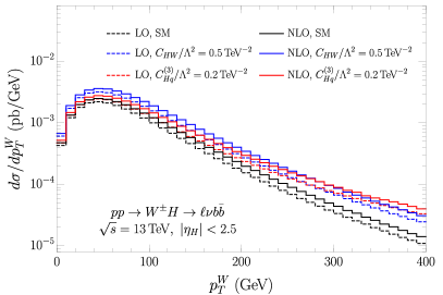
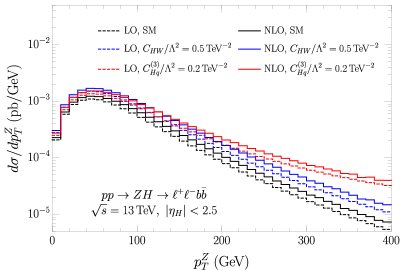
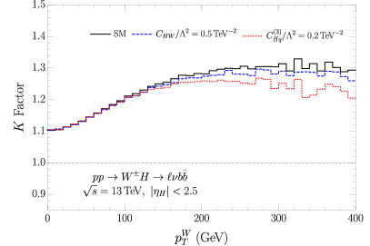
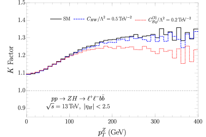
Figure 1: Top: Differential distributions for $W^{\pm}H$ (left) and $ZH$ (right) production at LO (dashed) and NLO (solid) in bins of $p_{T}^{V}$. We plot the results for the SM (black), $C_{HW}/\Lambda^{2}=0.5~{}\mathrm{TeV}^{-2}$ (blue), and $C_{Hq}^{(3)}/\Lambda^{2}=0.2~{}\mathrm{TeV}^{-2}$ (red). Bottom: The associated $K$-factors for the same distributions at the same three points, also in bins of $p_{T}^{V}$. The figures are computed to ${\cal{O}}(1/\Lambda^{4})$.

The effects of NLO QCD corrections in the SMEFT on distributions with anomalous couplings in $W^{+}W^{-}$ and $W^{\pm}Z$ production have been studied in previous work Baglio:2017bfe ; Baglio:2018bkm ; Baglio:2019uty . We now extend that analysis to include $W^{\pm}H$ and $ZH$ production Alioli:2018ljm . For $W^{+}W^{-}$ production, it was demonstrated in Refs. Baglio:2019uty ; Baglio:2017bfe ; Baglio:2018bkm that the $K$-factor — defined as the ratio of the NLO QCD (differential) cross section to the LO one — was largely unchanged by the presence of anomalous gauge and fermion couplings. For $W^{\pm}Z$ production, however, the effects of anomalous couplings on the $K$-factor were found to be quite large. This can be understood as the result of a delicate cancellation between the tree-level diagrams leading to $W^{\pm}Z$ production in the SM, which are intimately related to the presence of an approximate radiation zero Baur:1994ia in the tree-level amplitude. The radiation zero is spoiled by the presence of QCD radiation, leading to large $K$-factors Baglio:2013toa in some differential distributions. Because anomalous couplings affect the cancellation between the tree-level diagrams, the interplay of radiation and anomalous couplings makes an understanding of the NLO predictions crucial to obtain accurate predictions of the distributions at the LHC.

We now consider the interplay of QCD corrections and anomalous couplings on differential distributions for the associated production of a Higgs and a $W^{\pm}$ or $Z$ gauge boson Campanario:2014lza ; Granata:2017iod . While $W^{\pm}H$ and $ZH$ production do not have a tree-level radiation zero as in $W^{\pm}Z$ production, the longitudinal modes at high energy are closely related to the $W^{+}W^{-}$ and $W^{\pm}Z$ processes in the high-energy limit by the Goldstone theorem Grojean:2018dqj ; Panico:2017frx and so we expect interesting effects from QCD radiation.

In Fig. 1, we show the differential cross sections for $W^{\pm}H$ and $ZH$ production in bins of $p_{T}^{V}$ for the Standard Model and with $C_{HW}/\Lambda^{2}=0.5~{}\mathrm{TeV}^{-2}$ (blue) and $C_{Hq}^{(3)}/\Lambda^{2}=0.2~{}\mathrm{TeV}^{-2}$ (red). This figure includes the differential cross sections evaluated to ${\cal{O}}({1\over\Lambda^{4}})$. The NLO and LO predictions are shown as solid and dashed lines, respectively. In the lower panels, we show the corresponding $K$-factors at these benchmark points. At both LO and NLO, we see that the effects of $C_{Hq}^{(3)}$ grow fastest at high energy, due to the four-point interaction being unsuppressed by an $s$-channel vector boson propagator Biekotter:2018rhp ; Brehmer:2019gmn . For the anomalous-coupling points and for the SM, for both $W^{\pm}H$ and $ZH$ production, the $K$-factor becomes larger at high $p_{T}^{V}$, reaching $\sim 1.3$ for the SM at $400\,\mathrm{GeV}$. While less pronounced than the effects in $W^{\pm}Z$ production, treating the SMEFT contributions consistently at NLO QCD in the SMEFT changes the ratio of the NLO to LO predictions, and this has an effect on the fits to the distributions as we show in Section IV.

III.3 Angular Distributions and Gauge Boson Polarizations at NLO

We now turn to a discussion of the angular variables, $\cos\theta_{W}^{*}$ of the decayed charged leptons in the gauge boson rest frame. For $W^{\pm}Z$ production, we make use of the helicity coordinate system defined by ATLAS in Ref. Aaboud:2019gxl , defining the $z$-direction of the $W^{\pm}$ rest frame by the $W^{\pm}$ direction in the diboson center-of-mass frame. More details are given in Refs. Bern:2011ie ; Baglio:2018rcu . For $W^{\pm}H$ and $ZH$ production, we use the same variables, with the $W^{\pm}H$ or $ZH$ system replacing the $W^{\pm}Z$ center-of-mass frame, and the positively-charged lepton from the $Z$ decay playing the role of the charged lepton in the $W$ frame.

These angular variables are useful because their distributions are sensitive to the gauge boson polarizations Panico:2017frx . They are of particular interest to us here because of the relationship between the longitudinally polarized vector bosons and the Higgs boson. Understanding the polarization fractions for high-energy vector bosons has been shown to be a useful probe for anomalous-coupling measurements at the LHC Falkowski:2016cxu ; Panico:2017frx ; Franceschini:2017xkh . However, in Refs. Campanario:2014lza ; Baglio:2019uty it was found that the sensitivity of $\cos\theta_{W}^{*}$ to the anomalous couplings was lost in the presence of an extra jet. This is a manifestation of QCD corrections breaking the non-interference between helicity amplitudes of the SM and the dimension-6 SMEFT amplitudes, as originally pointed out in Ref. Dixon:1993xd , and studied in the context of electroweak interactions in Ref. Azatov:2017kzw . Here, we consider the impact of vetoing hard jets on restoring the sensitivity of these distributions at NLO.

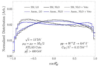
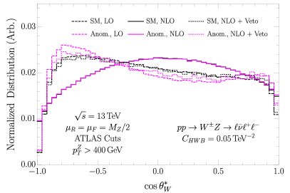
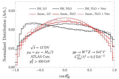
Figure 2: Normalized distributions of the angular variable, $\cos\theta_{W}^{*}$ in $WZ$ production at $13~{}\mathrm{TeV}$, requiring $p_{T}^{Z}>400\,\mathrm{GeV}$. In each figure we show the SM curve (black) for comparison along with an anomalous-coupling point: $C_{W}/\Lambda^{2}=0.15~{}\mathrm{TeV}^{-2}$ (upper left), $C_{HWB}/\Lambda^{2}=0.05~{}\mathrm{TeV}^{-2}$ (upper right), and $C_{Hq}^{(3)}/\Lambda^{2}=0.2~{}\mathrm{TeV}^{-2}$ (bottom). The points are chosen to be near the edge of the allowed regions by our combined fits to $WV$ and $VH$ production ($V=W^{\pm},Z$). For each parameter point, we plot the distribution at LO (dashed), NLO (solid), and at NLO with a jet veto (dotted). The jet veto curves correspond to a veto on jets with $p_{T}^{j}>150\,\mathrm{GeV}$. The figures are computed to ${\cal{O}}(1/\Lambda^{4})$.

In Fig. 2, we present the normalized $\cos\theta_{W}^{*}$ distributions from $W^{\pm}Z$ production at LO, NLO and at NLO with a $150\,\mathrm{GeV}$ jet veto. In all plots we also include a $p_{T}^{Z}$ cut, $p_{T}^{Z}>400$ GeV, in order to enhance our sensitivity to the anomalous couplings. In each figure we show the results for the SM as well as with one of three anomalous couplings: $C_{W}/\Lambda^{2}=0.15~{}\mathrm{TeV}^{-2}$ (upper left), $C_{HWB}/\Lambda^{2}=0.05~{}\mathrm{TeV}^{-2}$ (upper right), and $C_{Hq}^{(3)}/\Lambda^{2}=0.2~{}\mathrm{TeV}^{-2}$ (bottom). As is clear from comparing the LO (dashed) and NLO (solid) curves, the hard radiation present in $W^{\pm}Z$ production at NLO washes out much of the sensitivity to anomalous couplings, as the SM and anomalous-coupling curves are essentially indistinguishable at NLO, despite the differences at LO. With a veto on hard jets, however, the sensitivity is restored, essentially to the levels obtained at LO. At high energy, only the $(00)$ polarization (where both gauge bosons are longitudinally polarized) and $(\pm,\mp)$ (transverse polarizations) survive Baur:1994ia , and the angular distributions of the polarizations are different. The longitudinal polarization amplitude receives no contribution from the anomalous gauge couplings in the high-energy limit. Furthermore, only $C_{W}$ contributes to the high-energy limit of the $(\pm,\mp)$ amplitude. We also note that when only $C_{HWB}$ is turned on (pink curves, upper right in Fig. 2), the anomalous couplings $\lambda^{Z}=\lambda^{\gamma}$ are fixed to zero. Here, we can see that with the smaller value of $C_{HWB}$, the transverse contribution (which peaks at large $|\cos\theta_{W}^{*}|$) is enhanced, and the process is more sensitive to the $\delta g_{1}^{Z}$, $\delta\kappa^{\gamma}$ deviations than to the $\lambda^{Z}=\lambda^{\gamma}$ anomalous couplings.

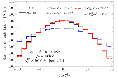
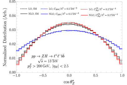
Figure 3: Normalized distributions of the angular variable $\cos\theta_{W}^{*}$ in $WH$ production (left) and $\cos\theta_{Z}^{*}$ in $ZH$ production (right), both at $13~{}\mathrm{TeV}$ and requiring the vector boson to have $p_{T}^{V}>200\,\mathrm{GeV}$ and the Higgs rapidity to lie within $\pm 2.5$. In each figure, we present the results at LO (dashed) and NLO (solid) for three different parameter points: the SM (black), with $C_{HW}/\Lambda^{2}=0.5~{}\mathrm{TeV}^{-2}$ (blue), and with $C_{Hq}^{(3)}/\Lambda^{2}=0.2~{}\mathrm{TeV}^{-2}$ (red). The figures are computed to ${\cal{O}}(1/\Lambda^{4})$.

In Fig. 3, we show the normalized distributions of the analogous angular variables but for $W^{\pm}H$ and $ZH$ production. We plot the results at LO (dashed) and NLO (solid) for $C_{HW}/\Lambda^{2}=0.5~{}\mathrm{TeV}^{-2}$ (blue) and $C_{Hq}^{(3)}/\Lambda^{2}=0.2~{}\mathrm{TeV}^{-2}$ (red). Here, we see that with $C_{Hq}^{(3)}$ nonzero, the distribution has a very similar shape to the SM piece, as both are dominated by the longitudinally polarized helicity amplitudes at high $p_{T}$. The distribution with nonzero $C_{HW}$, however, enhances the transverse parts of the amplitude, and thus has a shape that is enhanced at $\cos\theta_{V}^{*}=\pm 1$. This can be clearly seen in the LO results of Ref. Brehmer:2019gmn . In contrast to $W^{\pm}Z$, these distributions are largely unchanged by the higher-order corrections, and maintain their sensitivity to anomalous couplings that enhance the transverse polarizations even in the presence of radiation.

III.4 Sensitivity to Anomalous Couplings

We can also consider how the jet veto changes the sensitivity to anomalous couplings in other $W^{\pm}Z$ distributions. If we decompose a generic differential cross section up to $\mathcal{O}(\Lambda^{-4})$ as

$$\sigma(C_{i})=\sigma_{\textrm{SM}}+\Delta\sigma_{\Lambda^{2}}(C_{i})+\Delta\sigma_{\Lambda^{4}}(C_{i}^{2}),$$ (10)

we can isolate parts of the cross section that depend linearly and quadratically on the Wilson coefficients, and see how these parts grow with energy at LO, and in the presence of radiation. This is done in Fig. 4 for $W^{\pm}Z$ production with $C_{W}/\Lambda^{2}=0.15~{}\mathrm{TeV}^{-2}$ (top) and $C_{Hq}^{(3)}/\Lambda^{2}=0.2~{}\mathrm{TeV}^{-2}$ (bottom) in bins of $m_{T,WZ}$ for the $\Lambda^{-2}$ (left) and $\Lambda^{-4}$ (right) pieces, respectively.

We see immediately that the presence of QCD radiation makes a substantial difference in the sensitivity of the distributions to anomalous couplings. Focusing first on the linear pieces, we note that these arise from the interference between the dimension-6 SMEFT part of the amplitude with the SM part, and are thus subject to the non-interference effects noted in Refs. Falkowski:2016cxu ; Panico:2017frx ; Franceschini:2017xkh . At high energies, the SM amplitude receives contributions from both longitudinally and oppositely-polarized transverse gauge bosons. The portion of the amplitude proportional to $C_{W}$, however, has only transverse polarizations. The resulting non-interference between the SM and the dimension-6 SMEFT amplitudes is clear from the blue curve in Fig. 4 (upper left), which does not substantially grow with energy. As discussed in Ref. Azatov:2017kzw , however, the presence of an extra quark or gluon in the matrix element allows for this interference to be restored, and indeed, we see that the interference term at NLO (with or without a jet veto) grows substantially at high $m_{T}^{WZ}$. That this enhanced sensitivity to the interference persists even with a veto on the hard jets arising from the real emission implies that the virtual corrections play an important role in restoring the interference.

For the interference term proportional to $C_{Hq}^{(3)}$, the story is somewhat different. Here, we see that there is a growth in sensitivity at high energies even at LO, as the $C_{HQ}^{(3)}$ amplitude enhances the longitudinal parts of the amplitude which are already dominant in the SM part at high energies. At NLO, much of this sensitivity is washed out due to the presence of hard jets, but a great deal of the sensitivity can be restored by imposing a veto on the hard real emission.

Turning now to the $\mathcal{O}(\Lambda^{-4})$ terms, we see immediately on the right hand side of Fig.  4 that the LO distributions exhibit much faster growth with energy than the corresponding NLO curves, both for $C_{W}$ and $C_{Hq}^{(3)}$. The $\mathcal{O}(\Lambda^{-4})$ terms do not depend on any interference with the SM amplitude, so the sensitivity is dictated largely by the kinematics of the process. For anomalous gauge couplings, this was studied in Ref. Campanario:2014lza , where it was found that $W^{\pm}Z$ production at NLO generically allows for hard jets, which suppresses the sensitivity to the anomalous-coupling pieces (which grow like $({\text{Energy}})^{2}$). It was found there that much of the sensitivity in this distribution can be regained by vetoing events containing hard jets. The same conclusion is apparent both for $C_{W}$ and $C_{Hq}^{(3)}$ in Fig. 2, where vetoing jets with $p_{T}>150\,\mathrm{GeV}$ restores much of the sensitivity obtained at LO.

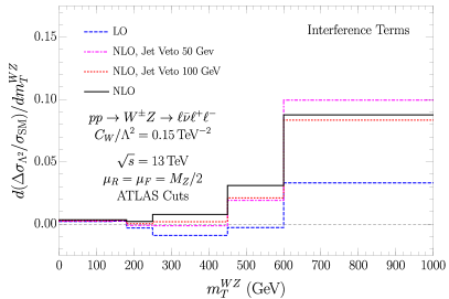
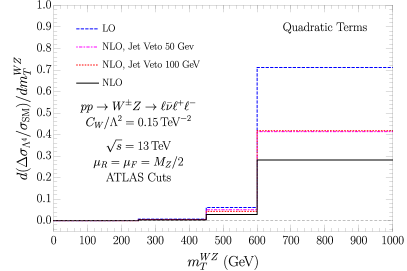
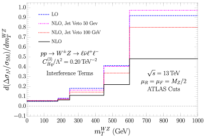
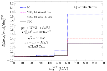
Figure 4: The sensitivity of the $m_{T}^{WZ}$ distributions to anomalous gauge (top) and fermion (botton) couplings, at LO and NLO with varying jet vetos. See text for details.

In principle, one could perform the same analysis on the $\mathcal{O}(\Lambda^{-2})$ and $\mathcal{O}(\Lambda^{-4})$ terms in the $W^{\pm}H$ distributions. In practice, though, the results are significantly less interesting when comparing LO to NLO. This is because, as shown in Ref. Campanario:2014lza , the real emission contributions to $W^{\pm}H$ production at NLO are typically soft, in contrast to the hard jets that appear in $W^{\pm}Z$ production. Thus, a veto on hard jets in $W^{\pm}H$ production at NLO does not significantly change the sensitivity to anomalous couplings, either at $\mathcal{O}(\Lambda^{-2})$ or $\mathcal{O}(\Lambda^{-4})$. Furthermore, as can be seen in Fig. 1, the $K$-factors are only mildly dependent on the anomalous couplings, so the sensitivity at LO and NLO to all higher-dimension operators is largely the same.

IV Fits to Warsaw Coefficients

IV.1 Datasets and Fitting Procedure

Section III.2 demonstrates that the implementation of NLO QCD within the SMEFT can have a significant impact on distributions. These changes lead to different predictions from those obtained by using LO QCD in the SMEFT with the appropriate Standard Model $K$-factor. We further solidify the need to include NLO QCD within SMEFT fits by showing the differences between fits with and without NLO. We also show that including $\mathcal{O}(1/\Lambda^{4})$ can significantly improve the fits. Lastly, the $\mathcal{O}(1/\Lambda^{4})$ terms allow one to explore if the values of coefficients are consistent with a weakly- or strongly-coupled theory.

We fit to the $10$ Warsaw basis coefficients described in Sect. II at both LO and NLO in the SMEFT to quantify these effects. We calculate uncorrelated $\chi^{2}$ fits to differential cross section measurements for the processes $W^{\pm}H,ZH,W^{+}W^{-}$, and $W^{\pm}Z$ and we construct the $\chi^{2}$ function for a given anomalous-coupling input, $\vec{C}$, as

$$\chi^{2}(\vec{C})=\sum_{\begin{subarray}{c}\text{\it WH, ZH}\\ \text{\it WW, WZ}\end{subarray}}^{\text{processes}}\sum_{\alpha}^{\text{datasets}}\sum_{i}^{\text{bins}}\frac{(\epsilon_{i\alpha}\hat{O}(\vec{C})_{i\alpha}^{\text{theory}}-\hat{O}_{i\alpha}^{\text{exp}})^{2}}{(v^{\text{exp}}_{i\alpha})^{2}}\,,$$ (11)

where $\hat{O}(\vec{C})_{i\alpha}^{\text{theory}}$, $\hat{O}_{i\alpha}^{\text{exp}}$, and $v^{\text{exp}}_{i\alpha}$ are respectively the theoretical expected value, experimental observation, and estimated uncertainties for the $i^{\text{th}}$ bin of dataset $\alpha$. An efficiency factor, $\epsilon_{i\alpha}$, is introduced to account for an overall scaling of the simulation data, where $\epsilon_{i\alpha}$ is calculated by taking the ratio of the experimentally simulated value for the SM differential cross section over our prediction for the differential cross section with an SM input ($\vec{C}=0$) for the $i^{\text{th}}$ bin of dataset $\alpha$.

The datasets that go into each process are detailed in Table 4. The uncertainties are estimated by combining reported statistical and systemic uncertainties in quadrature, assuming an overall 5% systematic uncertainty bin-by-bin, neglecting correlations.

Channel	Distribution	# bins	Data set	Int. Lum.
$W^{\pm}H\rightarrow b\bar{b}\ell^{\pm}+/\!\!\!\!E_{T}$	$p^{W}_{T}$, Fig. 3	2	ATLAS 8 TeV	79.8 fb-1 Aaboud:2019nan
$ZH\rightarrow b\bar{b}\ell^{+}\ell^{-}\text{ or }b\bar{b}+/\!\!\!\!E_{T}$	$p^{Z}_{T}$, Fig. 3	3	ATLAS 8 TeV	79.8 fb-1 Aaboud:2019nan
$W^{+}W^{-}\rightarrow\ell^{+}\ell^{\prime-}+/\!\!\!\!E_{T}\;(0j)$	$p^{\rm leading,lepton}_{T}$, Fig. 11	1	ATLAS 8 TeV	20.3 fb-1 Aad:2016wpd
$W^{+}W^{-}\rightarrow e^{\pm}\mu^{\mp}+/\!\!\!\!E_{T}\;(0j)$	$p_{T}^{\rm leading,lepton}$, Fig. 7	5	ATLAS 13 TeV	36.1 fb-1 Aaboud:2019nkz
$W^{\pm}Z\rightarrow\ell^{+}\ell^{-}\ell^{(\prime)\pm}$	$m_{T}^{WZ}$, Fig. 5	2	ATLAS 8 TeV	20.3 fb-1 Aad:2016ett
$W^{\pm}Z\rightarrow\ell^{+}\ell^{-}\ell^{(\prime)\pm}+/\!\!\!\!E_{T}$	$Z$ candidate $p_{T}^{\ell\ell}$, Fig. 5	9	CMS 8 TeV	19.6 fb-1 Khachatryan:2016poo
$W^{\pm}Z\rightarrow\ell^{+}\ell^{-}\ell^{(\prime)\pm}$	$m_{T}^{WZ}$ Fig. 4c	6	ATLAS 13 TeV	36.1 fb-1 Aaboud:2019gxl
$W^{\pm}Z\rightarrow\ell^{+}\ell^{-}\ell^{(\prime)\pm}+/\!\!\!\!E_{T}$	$m^{WZ}$, Fig. 15a	3	CMS 13 TeV,	35.9 fb-1 Sirunyan:2019bez

Table 4: Experimental data included in our study. The third column shows the number of bins used in our analysis, always counting from the highest.

We explore two methods for calculating confidence intervals of the Warsaw coefficients: projecting all but one coefficient to zero and alternatively profiling over the remaining coefficients to minimize the $\chi^{2}$ function at each point. The numerical results obtained by fitting all processes using both profiling and projecting are given in Table 5. They are compared graphically in Figures 5 and 6. Overall we see that the projected limits are significantly more stringent than the profiled. This is to be expected since the profiling allows for more flexibility in the $\chi^{2}$ function. The profiling method demonstrates the multidimensional nature of the fit.

We also show several 2D confidence interval fits using the projection method in Figure 7. In principle one could make a 2D confidence interval for each combination of Warsaw coefficients. However, most of these plots end up with similar results, showing order 20% NLO effects and with many of the regions falling in the strongly-coupled regime. We have selected some example plots that are particularly demonstrative and also correspond to interesting electroweak precision variables (S and T).

	$W^{+}W^{-}+W^{\pm}Z+ZH+W^{\pm}H$ Projected				$W^{+}W^{-}+W^{\pm}Z+ZH+W^{\pm}H$ Profiled
	$\Lambda^{-4}$		$\Lambda^{-2}$		$\Lambda^{-4}$		$\Lambda^{-2}$
	LO	NLO	LO	NLO	LO	NLO	LO	NLO
$C_{\text{HWB}}$	(-.05, .03)	(-.09, .04)	(-.07, .02)	(-.14, .03)	(-.70, .47)	(-.75, .50)	(-2.9, 2.3)	(-4.4, 1.5)
$C_{\text{Hq}}^{(3)}$	(-.02, .08)	(-.02, .11)	(-.02, .09)	(-.02, .14)	(-.26, .62)	(-.30, .67)	(-.17, .82)	(-.38, .82)
$C_{\text{HD}}$	(-.12, .06)	(-.21, .08)	(-.15, .05)	(-.30, .07)	(-1.1, 2.1)	(-1.2, 2.4)	(-4.5, 6.8)	(-2.6, 9.1)
$C_{\text{Hq}}^{(1)}$	(-.16, .21)	(-.18, .19)	(-.24, .20)	(-.32, .15)	(-.21, .38)	(-.25, .40)	(-.45, .93)	(-.81, .71)
$C_{\text{Hu}}$	(-.30, .22)	(-.33, .24)	(-.34, .72)	(-.38, .81)	(-.43, .59)	(-.46, .62)	(-23., 23.)	(-42., 48.)
$C_{\text{HW}}$	(-1.1, .55)	(-1.2, .56)	(-.52, .92)	(-.52, .92)	(-1.4, 2.4)	(-1.5, .51)	(-31., 19.)	(-33., 17.)
$C_{W}$	(-.13, .13)	(-.20, .18)	(-1.4, 1.3)	(-.28, .93)	(-.14, .14)	(-.20, .19)	(-1.3, 1.9)	(-3.2, 2.1)
$C_{\text{Hd}}$	(-.31, .35)	(-.33, .38)	(-2.2, 1.1)	(-2.2, 1.0)	(-.62, .45)	(-.67, .48)	(-82., 86.)	(-13., 14.)
$C_{H\square}$	(-4.9, 6.3)	(-4.9, 6.3)	(-4.6, 8.6)	(-4.6, 8.6)	(-57., 20.)	(-59., 20.)	(-27., 43.)	(-25., 43.)
$C_{\text{HB}}$	(-2.8, 2.3)	(-2.9, 2.4)	(-6.1, 11.)	(-6.0, 12.)	(-3.1, 3.8)	(-3.3, 4.0)	(-31., 22.)	(-31., 21.)

Table 5: $95\%$ confidence interval fits to individual EFT coefficients using $W^{+}W^{-}+W^{\pm}Z+ZH+W^{\pm}H$ data, with $\Lambda$ fixed to $1~{}\mathrm{TeV}$.

IV.2 Importance of NLO QCD and Quadratic Order Fits

The $95\%$ confidence intervals for the projected individual parameters are shown in Figure 5. We have included solid (dashed) grey lines at $\pm 0.5(1.0)$ to guide the eye. Similarly, we show the individual $95\%$ confidence intervals from the profiled fitting procedure in Figure 6. The solid (dashed) lines are now at $\pm 2.0(4.0)$ and the scales have been expanded. Black (blue) lines indicate that we are working to LO (NLO) QCD in the SMEFT, and solid (dashed) lines indicate the expansion to $\mathcal{O}(\frac{1}{\Lambda^{4}})$ ( $\mathcal{O}(\frac{1}{\Lambda^{2}})$ ).

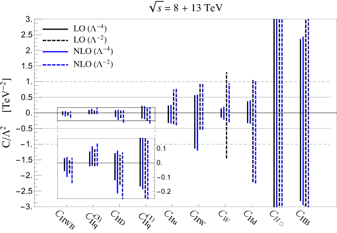
Figure 5: $95\%$ confidence interval fits to individual EFT coefficients using $W^{+}W^{-}+W^{\pm}Z+ZH+W^{\pm}H$ data. All other SMEFT coefficients are projected to zero. Fits quadratic in $1/\Lambda^{2}$ (Linear) LO and NLO QCD are shown as solid (dashed), black and blue lines respectively.

Similarly, we show the $95\%$ confidence intervals for some selected planes of parameters using the projected method in Figure 7 for LO (inside black curve ) and NLO (inside blue curve) QCD in the SMEFT, along with the limits from Electroweak Precision Observables (EWPO) Falkowski:2014tna (inside red curve) to $\mathcal{O}(\frac{1}{\Lambda^{4}})$, using the $\chi^{2}$ fit of Ref. Dawson:2019clf . Again, we emphasize that our results are not meant to compete with the global fits including Higgs data and EWPO, but rather, our goal is to determine the importance of NLO QCD within the SMEFT and to examine the $1/\Lambda^{2}$ dependence. The EWPO curves are included, however, as a reference for comparison.

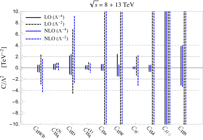
Figure 6: $95\%$ confidence interval fits to individual EFT coefficients using $W^{+}W^{-}+W^{\pm}Z+ZH+W^{\pm}H$ data and profiling over all other coefficients. Fits quadratic in $1/\Lambda^{2}$ (Linear) LO and NLO QCD are shown as solid (dashed) black and blue lines respectively.

First, let us compare the differences of the LO and NLO QCD fits in the SMEFT, the black and blue lines. Looking at the results in Figures 5 and 6, including NLO QCD in the SMEFT can change the fit intervals on the order of $10-20\%$, on average. For some coefficients, NLO QCD can have an effect as large as $50\%$. From the two-dimensional plots in Figure 7, we see that going from LO to NLO QCD can shift the curves by as much as $25\%$ in some directions, along with altering the overall orientation and shapes of the curves.

Next we compare the differences in the fits when working to $\mathcal{O}(\frac{1}{\Lambda^{4}})$ versus $\mathcal{O}(\frac{1}{\Lambda^{2}})$, the solid and dashed lines. The $\mathcal{O}(\frac{1}{\Lambda^{4}})$ fits are always better or comparable to the $\mathcal{O}(\frac{1}{\Lambda^{2}})$ fits. On average, working to $\mathcal{O}(\frac{1}{\Lambda^{4}})$ improves the fits by a factor of two and as much as a factor of ten in some of the profiled fits. Such a large improvement in the fit hints that the coefficients no longer correspond to a weakly-coupled theory and we discuss this in more detail in the following section. Similar results when comparing the $\mathcal{O}(\frac{1}{\Lambda^{4}})$ fits to those obtained at $\mathcal{O}(\frac{1}{\Lambda^{2}})$ were obtained in Ref. Almeida:2018cld at LO QCD.

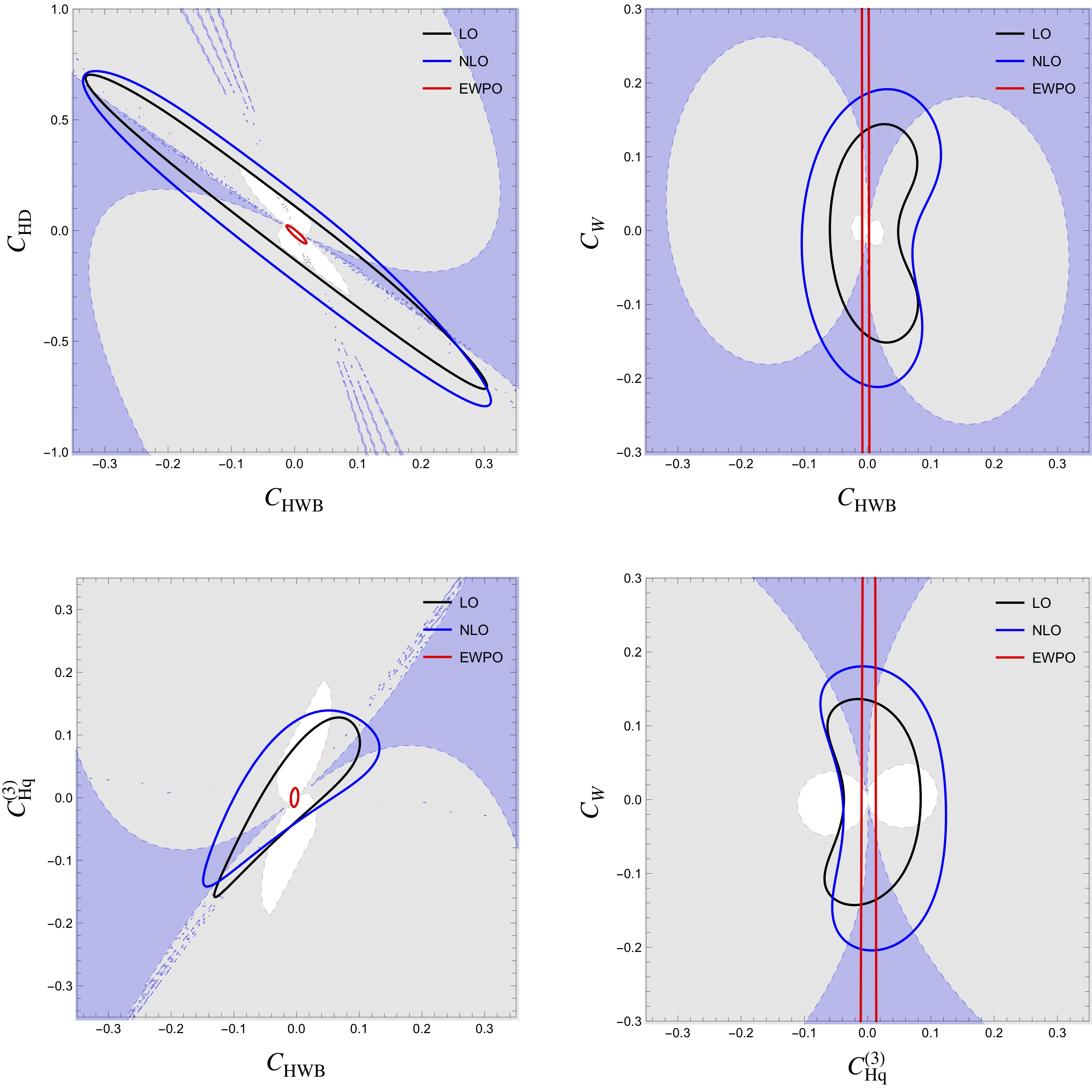
Figure 7: 95 % confidence region in the $C_{HWB}-C_{HD}$ (top left) , $C_{HWB}-C_{W}$ (top right), $C_{HWB}-C_{Hq}^{(3)}$ (bottom left), and $C_{Hq}^{(3)}-C_{W}$ (bottom right) planes with all other EFT coefficients projected to zero and $\Lambda$ fixed to $1~{}\mathrm{TeV}$. Quadratic fits to $W^{+}W^{-}+W^{\pm}Z+ZH+W^{\pm}H$ distributions are shown in black (blue) for LO (NLO) QCD in SMEFT, while the quadratic fit to NLO Electroweak Precision Observables is shown in red. The grey (blue) region indicates the coefficients no longer correspond to a weakly-coupled theory that is $\Delta\sigma_{\Lambda^{4}}>\Delta\sigma_{\Lambda^{2}}~{}(4\pi\Delta\sigma_{\Lambda^{2}})$.

IV.3 The Validity of Weakly-Coupled Theory

We decompose the differential cross sections as in Eq. 10 . The SMEFT couplings generically scale as $\alpha_{\text{EFT}}\sim\frac{g_{\text{EFT}}^{2}v^{2}}{\Lambda^{2}}$ or $\frac{g_{\text{EFT}}^{2}{\text{Energy}}^{2}}{\Lambda^{2}}$, where $g_{EFT}$ parameterizes the strength of the underlying UV complete theory. The linear piece, $\Delta\sigma_{\Lambda^{2}}$, goes as $\mathcal{O}(\alpha_{\text{EFT}})$, and the quadratic piece $\Delta\sigma_{\Lambda^{4}}$ goes as $\mathcal{O}(\alpha_{\text{EFT}}^{2})$. In a weakly-coupled theory, one generically expects $\alpha_{\text{EFT}}\lesssim 1$. This implies $\Delta\sigma_{\Lambda^{4}}/\Delta\sigma_{\Lambda^{2}}\lesssim 1$ for a weakly-coupled theory, assuming that there are no cancellations in the underlying UV theory. Alternatively, one might also consider the upper limit on a weakly-coupled theory to be $\alpha_{\text{EFT}}\lesssim 4\pi$ as some sort of perturbative unitarity bound. Similar criterion have been explored elsewhere in the literature Contino:2016jqw .

In Fig. 7, we show different regions detailing the strength of the coupling by comparing the differential cross sections in each bin. All parameters not shown in the plot are projected to zero. The white regions in the figures indicate that $\Delta\sigma_{\Lambda^{4}}/\Delta\sigma_{\Lambda^{2}}<1$ for all bins in all of the processes considered. One may consider this the weakly-coupled regime. The grey and blue regions respectively indicate that $\Delta\sigma_{\Lambda^{4}}/\Delta\sigma_{\Lambda^{2}}>1$ and $\Delta\sigma_{\Lambda^{4}}/\Delta\sigma_{\Lambda^{2}}>4\pi$ in at least one bin for at least one process. Any coefficient or fit in these regions would no longer be considered part of a weakly-coupled theory.

We see in Fig. 7 that many of the confidence intervals we derived for the $WV+VH$ data (within the blue or black curves) fall within a grey shaded region. If the coefficients lie in this area they correspond to a strongly-interacting theory and higher-dimension operators need to be retained. In contrast, the bounds from the EWPO (within the red curves) place strong constraints on the couplings and typically fall within the weakly-coupled regime (white region). One might consider setting an experimental goal of LHC to have all fits sufficiently precise such that they could probe the weakly-coupled regime. In this way one could fully understand the fits in terms of dimension-6 operators.

There are small regions protruding into some of the regions within the plots. They are particularly evident in the top left plot in Figure 7. These can be seen in other plots not displayed here. They can be understood as cancellations within the helicity amplitudes.

We also note that as Warsaw coefficients are increased, the last bin will be the first indication that the weakly-coupled theory is no longer valid. The argument is similar to those made in previous works showing that most of the fitting power comes from the last bin Brehmer:2019gmn . We know SM cross sections are falling with increasing energy, while the quadratic SMEFT piece grows with energy. Therefore the bin with the largest energy, the last one, will have the largest deviation from the SM and best fitting power.

V Conclusion

As the quest for discovering beyond-Standard-Model particles continues without any direct observations, it is important to understand all the data we have to the best precision. Such precision measurements could be the first evidence for some new high-scale physics. To this end, we have studied the effects of NLO QCD in the SMEFT on the $W^{+}W^{-},W^{\pm}Z,W^{\pm}H$, and $ZH$ production at the LHC. We find that including QCD radiation can have a significant effect on the parameters. This implies that global SMEFT fits including Higgs data and EWPO need to be done beyond LO in QCD. We have also explored the numerical differences between the $1/\Lambda^{2}$ and $1/\Lambda^{4}$ fits. Their differences suggest that current fits to LHC data are not yet sensitive to weakly-coupled theories for the majority of coefficients.

Primitive cross sections at $8$ and $13$ TeV for $W^{\pm}Z$ production with jet vetos, and at $13$ TeV for $W^{\pm}H$ production are posted at https://quark.phy.bnl.gov/Digital_Data_Archive/dawson/VV_20.

Appendix A Numerical Fits

We show tables detailing the numerical results of the $95\%$ confidence intervals to different subsets of processes in Tables 6,  7, and  8. Entries with a ”-” mean no fit was performed, since the process does not depend on that parameter. Overall, fitting to a few bins in $W^{\pm}H$ and $ZH$ processes yields comparable sensitivity to that of the $W^{+}W^{-}$and $W^{\pm}Z$ fits for some parameters.

	$W^{\pm}H$ Projected				$ZH$ Projected
	$\Lambda^{-4}$		$\Lambda^{-2}$		$\Lambda^{-4}$		$\Lambda^{-2}$
	LO	NLO	LO	NLO	LO	NLO	LO	NLO
$C_{\text{HWB}}$	-	-	-	-	(-3.1, 1.8)	(-3.3, 1.8)	(-1.8, 3.4)	(-1.8, 3.4)
$C_{\text{Hq}}^{(3)}$	(-.61, .19)	(-.65, .20)	(-.20, .26)	(-.22, .29)	(-.33, .12)	(-.35, .13)	(-.08, .18)	(-.09, .20)
$C_{\text{HD}}$	(-33., 16.)	(-33., 16.)	(-63., 53.)	(-63., 53.)	(-17., 21.)	(-17., 21.)	(-14., 26.)	(-14., 26.)
$C_{\text{Hq}}^{(1)}$	-	-	-	-	(-.20, .22)	(-.21, .24)	(-1.9, .77)	(-2.0, .82)
$C_{\text{Hu}}$	-	-	-	-	(-.31, .22)	(-.34, .24)	(-.33, .76)	(-.37, .85)
$C_{\text{HW}}$	(-1.2, .59)	(-1.2, .61)	(-.96, 1.1)	(-.96, 1.1)	(-1.5, .75)	(-1.5, .77)	(-.69, 1.3)	(-.69, 1.3)
$C_{W}$	-	-	-	-	-	-	-	-
$C_{\text{Hd}}$	-	-	-	-	(-.31, .36)	(-.34, .39)	(-2.3, 1.)	(-2.3, 1.0)
$C_{H\square}$	(-41., 8.2)	(-41., 8.2)	(-13., 16.)	(-13., 16.)	(-6.5, 7.8)	(-6.5, 7.8)	(-5.2, 9.7)	(-5.2, 9.7)
$C_{\text{HB}}$	-	-	-	-	(-2.8, 2.3)	(-2.9, 2.4)	(-6.1, 11.)	(-6.0, 12.)

Table 6: $95\%$ confidence interval fits to individual EFT coefficients using $W^{\pm}H$ and $ZH$ data, with $\Lambda$ fixed to $1~{}\mathrm{TeV}$.

	$W^{+}W^{-}$ Projected				$W^{\pm}Z$ Projected
	$\Lambda^{-4}$		$\Lambda^{-2}$		$\Lambda^{-4}$		$\Lambda^{-2}$
	LO	NLO	LO	NLO	LO	NLO	LO	NLO
$C_{\text{HWB}}$	(-.14, .17)	(-.14, .18)	(-.35, .38)	(-.37, .4)	(-.05, .03)	(-.1, .03)	(-.07, .02)	(-.14, .03)
$C_{\text{Hq}}^{(3)}$	(-.34, .21)	(-.35, .22)	(-.33, .3)	(-.35, .32)	(-.03, .08)	(-.03, .15)	(-.03, .1)	(-.03, .18)
$C_{\text{HD}}$	(-.35, .54)	(-.36, .56)	(-.60, .69)	(-.64, .73)	(-.12, .06)	(-.22, .07)	(-.15, .05)	(-.32, .06)
$C_{\text{Hq}}^{(1)}$	(-.37, .34)	(-.38, .35)	(-4.8, 3.1)	(-5.4, 3.4)	(-.26, 1.7)	(-1.5, .43)	(-.15, 2.8)	(-1.3, .45)
$C_{\text{Hu}}$	(-.47, .41)	(-.48, .42)	(-3.1, 2.4)	(-3.4, 2.6)	-	-	-	-
$C_{\text{HW}}$	-	-	-	-	-	-	-	-
$C_{W}$	(-.22, .23)	(-.23, .23)	(-4.4, 5.1)	(-9.6, 6.8)	(-.14, .13)	(-.22, .19)	(-1.5, 1.3)	(-.27, .94)
$C_{\text{Hd}}$	(-.59, .62)	(-.59, .63)	(-7.6, 9.7)	(-8.0, 10.)	-	-	-	-
$C_{H\square}$	-	-	-	-	-	-	-	-
$C_{\text{HB}}$	-	-	-	-	-	-	-	-

Table 7: The same as Table 6, but using $W^{+}W^{-}$ and $W^{\pm}Z$ data, with $\Lambda$ fixed to $1~{}\mathrm{TeV}$

	$ZH+W^{\pm}H$ Projected				$W^{+}W^{-}+W^{\pm}Z$ Projected
	$\Lambda^{-4}$		$\Lambda^{-2}$		$\Lambda^{-4}$		$\Lambda^{-2}$
	LO	NLO	LO	NLO	LO	NLO	LO	NLO
$C_{\text{HWB}}$	(-3.1, 1.8)	(-3.3, 1.8)	(-1.8, 3.4)	(-1.8, 3.4)	(-.05, .03)	(-.09, .04)	(-.07, .02)	(-.14, .03)
$C_{\text{Hq}}^{(3)}$	(-.32, .12)	(-.34, .13)	(-.07, .16)	(-.07, .18)	(-.03, .08)	(-.03, .14)	(-.03, .10)	(-.03, .17)
$C_{\text{HD}}$	(-16., 19.)	(-16., 19.)	(-14., 24.)	(-14., 24.)	(-.12, .06)	(-.21, .08)	(-.15, .05)	(-.30, .07)
$C_{\text{Hq}}^{(1)}$	(-.17, .21)	(-.18, .23)	(-.27, .18)	(-.30, .20)	(-.31, .37)	(-.40, .28)	(-.33, 2.5)	(-1.3, .41)
$C_{\text{Hu}}$	(-.31, .22)	(-.34, .24)	(-.33, .76)	(-.37, .85)	(-.47, .41)	(-.48, .42)	(-3.1, 2.4)	(-3.4, 2.6)
$C_{\text{HW}}$	(-1.1, .55)	(-1.2, .56)	(-.52, .92)	(-.52, .92)	-	-	-	-
$C_{W}$	-	-	-	-	(-.13, .13)	(-.20, .18)	(-1.4, 1.3)	(-.28, .93)
$C_{\text{Hd}}$	(-.31, .36)	(-.34, .39)	(-2.3, 1.0)	(-2.3, 1.0)	(-.59, .62)	(-.59, .63)	(-7.6, 9.7)	(-8.0, 10.)
$C_{H\square}$	(-4.9, 6.3)	(-4.9, 6.3)	(-4.6, 8.6)	(-4.6, 8.6)	-	-	-	-
$C_{\text{HB}}$	(-2.8, 2.3)	(-2.9, 2.4)	(-6.1, 11.)	(-6.0, 12.)	-	-	-	-

Table 8: The same as Table 6, but using $ZH+W^{\pm}H$ and $W^{+}W^{-}+W^{\pm}Z$ data, with $\Lambda$ fixed to $1~{}\mathrm{TeV}$.

References

- (1) E. da Silva Almeida, A. Alves, N. Rosa Agostinho, O. J. P. Éboli, and M. C. Gonzalez-Garcia, “Electroweak Sector Under Scrutiny: A Combined Analysis of LHC and Electroweak Precision Data,” Phys. Rev. D99 no. 3, (2019) 033001, arXiv:1812.01009 [hep-ph].
- (2) A. Biekotter, T. Corbett, and T. Plehn, “The Gauge-Higgs Legacy of the LHC Run II,” SciPost Phys. 6 (2019) 064, arXiv:1812.07587 [hep-ph].
- (3) C. Grojean, M. Montull, and M. Riembau, “Diboson at the LHC vs LEP,” JHEP 03 (2019) 020, arXiv:1810.05149 [hep-ph].
- (4) J. Ellis, C. W. Murphy, V. Sanz, and T. You, “Updated Global SMEFT Fit to Higgs, Diboson and Electroweak Data,” JHEP 06 (2018) 146, arXiv:1803.03252 [hep-ph].
- (5) L. Berthier, M. Bjorn, and M. Trott, “Incorporating doubly resonant data in a global fit of SMEFT parameters to lift flat directions,” JHEP 09 (2016) 157, arXiv:1606.06693 [hep-ph].
- (6) I. Brivio and M. Trott, “The Standard Model as an Effective Field Theory,” Phys. Rept. 793 (2019) 1–98, arXiv:1706.08945 [hep-ph].
- (7) A. Falkowski, M. Gonzalez-Alonso, A. Greljo, D. Marzocca, and M. Son, “Anomalous Triple Gauge Couplings in the Effective Field Theory Approach at the LHC,” JHEP 02 (2017) 115, arXiv:1609.06312 [hep-ph].
- (8) W. Buchmuller and D. Wyler, “Effective Lagrangian Analysis of New Interactions and Flavor Conservation,” Nucl. Phys. B268 (1986) 621–653.
- (9) B. Grzadkowski, M. Iskrzynski, M. Misiak, and J. Rosiek, “Dimension-Six Terms in the Standard Model Lagrangian,” JHEP 10 (2010) 085, arXiv:1008.4884 [hep-ph].
- (10) J. Baglio, S. Dawson, and I. M. Lewis, “An NLO QCD effective field theory analysis of production at the LHC including fermionic operators,” Phys. Rev. D96 no. 7, (2017) 073003, arXiv:1708.03332 [hep-ph].
- (11) J. Baglio, S. Dawson, and I. M. Lewis, “NLO effects in EFT fits to production at the LHC,” Phys. Rev. D99 no. 3, (2019) 035029, arXiv:1812.00214 [hep-ph].
- (12) J. Baglio, S. Dawson, and S. Homiller, “QCD corrections in Standard Model EFT fits to and production,” Phys. Rev. D100 no. 11, (2019) 113010, arXiv:1909.11576 [hep-ph].
- (13) S. Alioli, W. Dekens, M. Girard, and E. Mereghetti, “NLO QCD corrections to SM-EFT dilepton and electroweak Higgs boson production, matched to parton shower in POWHEG,” JHEP 08 (2018) 205, arXiv:1804.07407 [hep-ph].
- (14) T. Melia, P. Nason, R. Rontsch, and G. Zanderighi, “W+W-, WZ and ZZ production in the POWHEG BOX,” JHEP 11 (2011) 078, arXiv:1107.5051 [hep-ph].
- (15) P. Nason and G. Zanderighi, “ , and production in the POWHEG-BOX-V2,” Eur. Phys. J. C74 no. 1, (2014) 2702, arXiv:1311.1365 [hep-ph].
- (16) G. Luisoni, P. Nason, C. Oleari, and F. Tramontano, “/HZ + 0 and 1 jet at NLO with the POWHEG BOX interfaced to GoSam and their merging within MiNLO,” JHEP 10 (2013) 083, arXiv:1306.2542 [hep-ph].
- (17) S. Frixione, P. Nason, and C. Oleari, “Matching NLO QCD computations with Parton Shower simulations: the POWHEG method,” JHEP 11 (2007) 070, arXiv:0709.2092 [hep-ph].
- (18) S. Alioli, P. Nason, C. Oleari, and E. Re, “A general framework for implementing NLO calculations in shower Monte Carlo programs: the POWHEG BOX,” JHEP 06 (2010) 043, arXiv:1002.2581 [hep-ph].
- (19) J. Ohnemus, “An Order calculation of hadronic production,” Phys. Rev. D44 (1991) 1403–1414.
- (20) J. Ohnemus, “An Order calculation of hadronic production,” Phys. Rev. D44 (1991) 3477–3489.
- (21) S. Frixione, P. Nason, and G. Ridolfi, “Strong corrections to W Z production at hadron colliders,” Nucl. Phys. B383 (1992) 3–44.
- (22) J. Ohnemus, “Hadronic , , and production with QCD corrections and leptonic decays,” Phys. Rev. D50 (1994) 1931–1945, arXiv:hep-ph/9403331 [hep-ph].
- (23) L. J. Dixon, Z. Kunszt, and A. Signer, “Helicity amplitudes for O(alpha-s) production of , , , , or pairs at hadron colliders,” Nucl. Phys. B531 (1998) 3–23, arXiv:hep-ph/9803250 [hep-ph].
- (24) J. M. Campbell and R. K. Ellis, “An Update on vector boson pair production at hadron colliders,” Phys. Rev. D60 (1999) 113006, arXiv:hep-ph/9905386 [hep-ph].
- (25) J. M. Campbell, R. K. Ellis, and C. Williams, “Vector boson pair production at the LHC,” JHEP 07 (2011) 018, arXiv:1105.0020 [hep-ph].
- (26) T. Han and S. Willenbrock, “QCD correction to the and total cross-sections,” Phys. Lett. B273 (1991) 167–172.
- (27) J. Ohnemus and W. J. Stirling, “Order corrections to the differential cross-section for the intermediate mass Higgs signal,” Phys. Rev. D47 (1993) 2722–2729.
- (28) H. Baer, B. Bailey, and J. F. Owens, “ Monte Carlo approach to W + Higgs associated production at hadron supercolliders,” Phys. Rev. D47 (1993) 2730–2734.
- (29) A. Stange, W. J. Marciano, and S. Willenbrock, “Associated production of Higgs and weak bosons, with , at hadron colliders,” Phys. Rev. D50 (1994) 4491–4498, arXiv:hep-ph/9404247 [hep-ph].
- (30) T. Gehrmann, M. Grazzini, S. Kallweit, P. Maierhofer, A. von Manteuffel, S. Pozzorini, D. Rathlev, and L. Tancredi, “ Production at Hadron Colliders in Next to Next to Leading Order QCD,” Phys. Rev. Lett. 113 no. 21, (2014) 212001, arXiv:1408.5243 [hep-ph].
- (31) F. Caola, K. Melnikov, R. Rontsch, and L. Tancredi, “QCD corrections to production through gluon fusion,” Phys. Lett. B754 (2016) 275–280, arXiv:1511.08617 [hep-ph].
- (32) M. Grazzini, S. Kallweit, D. Rathlev, and M. Wiesemann, “ production at hadron colliders in NNLO QCD,” Phys. Lett. B761 (2016) 179–183, arXiv:1604.08576 [hep-ph].
- (33) O. Brein, A. Djouadi, and R. Harlander, “NNLO QCD corrections to the Higgs-strahlung processes at hadron colliders,” Phys. Lett. B579 (2004) 149–156, arXiv:hep-ph/0307206 [hep-ph].
- (34) G. Ferrera, M. Grazzini, and F. Tramontano, “Associated WH production at hadron colliders: a fully exclusive QCD calculation at NNLO,” Phys. Rev. Lett. 107 (2011) 152003, arXiv:1107.1164 [hep-ph].
- (35) G. Ferrera, M. Grazzini, and F. Tramontano, “Associated ZH production at hadron colliders: the fully differential NNLO QCD calculation,” Phys. Lett. B740 (2015) 51–55, arXiv:1407.4747 [hep-ph].
- (36) J. M. Campbell, R. K. Ellis, and C. Williams, “Associated production of a Higgs boson at NNLO,” JHEP 06 (2016) 179, arXiv:1601.00658 [hep-ph].
- (37) J. Baglio, L. D. Ninh, and M. M. Weber, “Massive gauge boson pair production at the LHC: a next-to-leading order story,” Phys. Rev. D88 (2013) 113005, arXiv:1307.4331 [hep-ph]. [Erratum: Phys. Rev.D94,no.9,099902(2016)].
- (38) A. Bierweiler, T. Kasprzik, and J. H. Kuhn, “Vector-boson pair production at the LHC to accuracy,” JHEP 12 (2013) 071, arXiv:1305.5402 [hep-ph].
- (39) M. Billoni, S. Dittmaier, B. Jager, and C. Speckner, “Next-to-leading order electroweak corrections to 4 leptons at the LHC in double-pole approximation,” JHEP 12 (2013) 043, arXiv:1310.1564 [hep-ph].
- (40) B. Biedermann, M. Billoni, A. Denner, S. Dittmaier, L. Hofer, B. Jäger, and L. Salfelder, “Next-to-leading-order electroweak corrections to 4 leptons at the LHC,” JHEP 06 (2016) 065, arXiv:1605.03419 [hep-ph].
- (41) B. Biedermann, A. Denner, and L. Hofer, “Next-to-leading-order electroweak corrections to the production of three charged leptons plus missing energy at the LHC,” JHEP 10 (2017) 043, arXiv:1708.06938 [hep-ph].
- (42) J. Baglio and N. Le Duc, “Fiducial polarization observables in hadronic WZ production: A next-to-leading order QCD+EW study,” JHEP 04 (2019) 065, arXiv:1810.11034 [hep-ph].
- (43) M. Grazzini, S. Kallweit, J. M. Lindert, S. Pozzorini, and M. Wiesemann, “NNLO QCD + NLO EW with Matrix+OpenLoops: precise predictions for vector-boson pair production,” JHEP 02 (2020) 087, arXiv:1912.00068 [hep-ph].
- (44) A. Denner, S. Dittmaier, S. Kallweit, and A. Muck, “Electroweak corrections to Higgs-strahlung off W/Z bosons at the Tevatron and the LHC with HAWK,” JHEP 03 (2012) 075, arXiv:1112.5142 [hep-ph].
- (45) K. Hagiwara, R. D. Peccei, D. Zeppenfeld, and K. Hikasa, “Probing the Weak Boson Sector in ,” Nucl. Phys. B282 (1987) 253–307.
- (46) K. Hagiwara, R. Szalapski, and D. Zeppenfeld, “Anomalous Higgs boson production and decay,” Phys. Lett. B318 (1993) 155–162, arXiv:hep-ph/9308347 [hep-ph].
- (47) U. Baur, T. Han, and J. Ohnemus, “ production at hadron colliders: Effects of nonstandard couplings and QCD corrections,” Phys. Rev. D51 (1995) 3381–3407, arXiv:hep-ph/9410266 [hep-ph].
- (48) U. Baur, T. Han, and J. Ohnemus, “QCD corrections and nonstandard three vector boson couplings in production at hadron colliders,” Phys. Rev. D53 (1996) 1098–1123, arXiv:hep-ph/9507336 [hep-ph].
- (49) L. J. Dixon, Z. Kunszt, and A. Signer, “Vector boson pair production in hadronic collisions at order : Lepton correlations and anomalous couplings,” Phys. Rev. D60 (1999) 114037, arXiv:hep-ph/9907305 [hep-ph].
- (50) M. Chiesa, A. Denner, and J.-N. Lang, “Anomalous triple-gauge-boson interactions in vector-boson pair production with RECOLA2,” Eur. Phys. J. C78 no. 6, (2018) 467, arXiv:1804.01477 [hep-ph].
- (51) F. Campanario, R. Roth, and D. Zeppenfeld, “QCD radiation in and production and anomalous coupling measurements,” Phys. Rev. D91 (2015) 054039, arXiv:1410.4840 [hep-ph].
- (52) F. Granata, J. M. Lindert, C. Oleari, and S. Pozzorini, “NLO QCD+EW predictions for HV and HV +jet production including parton-shower effects,” JHEP 09 (2017) 012, arXiv:1706.03522 [hep-ph].
- (53) A. Azatov, D. Barducci, and E. Venturini, “Precision diboson measurements at hadron colliders,” JHEP 04 (2019) 075, arXiv:1901.04821 [hep-ph].
- (54) R. Contino, A. Falkowski, F. Goertz, C. Grojean, and F. Riva, “On the Validity of the Effective Field Theory Approach to SM Precision Tests,” JHEP 07 (2016) 144, arXiv:1604.06444 [hep-ph].
- (55) C. Hays, A. Martin, V. Sanz, and J. Setford, “On the impact of dimension-eight SMEFT operators on Higgs measurements,” JHEP 02 (2019) 123, arXiv:1808.00442 [hep-ph].
- (56) S. Alte, M. Konig, and W. Shepherd, “Consistent Searches for SMEFT Effects in Non-Resonant Dilepton Events,” JHEP 07 (2019) 144, arXiv:1812.07575 [hep-ph].
- (57) A. Falkowski, M. Gonzalez-Alonso, A. Greljo, and D. Marzocca, “Global constraints on anomalous triple gauge couplings in effective field theory approach,” Phys. Rev. Lett. 116 no. 1, (2016) 011801, arXiv:1508.00581 [hep-ph].
- (58) R. Franceschini, G. Panico, A. Pomarol, F. Riva, and A. Wulzer, “Electroweak Precision Tests in High-Energy Diboson Processes,” JHEP 02 (2018) 111, arXiv:1712.01310 [hep-ph].
- (59) D. Liu and L.-T. Wang, “Prospects for precision measurement of diboson processes in the semileptonic decay channel in future LHC runs,” Phys. Rev. D99 no. 5, (2019) 055001, arXiv:1804.08688 [hep-ph].
- (60) A. Falkowski, B. Fuks, K. Mawatari, K. Mimasu, F. Riva, and V. Sanz, “Rosetta: an operator basis translator for Standard Model effective field theory,” Eur. Phys. J. C75 no. 12, (2015) 583, arXiv:1508.05895 [hep-ph].
- (61) A. Dedes, W. Materkowska, M. Paraskevas, J. Rosiek, and K. Suxho, “Feynman rules for the Standard Model Effective Field Theory in Rξ-gauges,” JHEP 06 (2017) 143, arXiv:1704.03888 [hep-ph].
- (62) I. Brivio and M. Trott, “Scheming in the SMEFT… and a reparameterization invariance!,” JHEP 07 (2017) 148, arXiv:1701.06424 [hep-ph]. [Addendum: JHEP05,136(2018)].
- (63) E. E. Jenkins, A. V. Manohar, and P. Stoffer, “Low-Energy Effective Field Theory below the Electroweak Scale: Operators and Matching,” JHEP 03 (2018) 016, arXiv:1709.04486 [hep-ph].
- (64) Z. Zhang, “Time to Go Beyond Triple-Gauge-Boson-Coupling Interpretation of Pair Production,” Phys. Rev. Lett. 118 no. 1, (2017) 011803, arXiv:1610.01618 [hep-ph].
- (65) L. Berthier and M. Trott, “Towards consistent Electroweak Precision Data constraints in the SMEFT,” JHEP 05 (2015) 024, arXiv:1502.02570 [hep-ph].
- (66) R. S. Gupta, A. Pomarol, and F. Riva, “BSM Primary Effects,” Phys. Rev. D91 no. 3, (2015) 035001, arXiv:1405.0181 [hep-ph].
- (67) A. Falkowski, “Effective field theory approach to LHC Higgs data,” Pramana 87 no. 3, (2016) 39, arXiv:1505.00046 [hep-ph].
- (68) Particle Data Group Collaboration, M. Tanabashi et al., “Review of Particle Physics,” Phys. Rev. D98 no. 3, (2018) 030001.
- (69) S. Alioli, V. Cirigliano, W. Dekens, J. de Vries, and E. Mereghetti, “Right-handed charged currents in the era of the Large Hadron Collider,” JHEP 05 (2017) 086, arXiv:1703.04751 [hep-ph].
- (70) U. Baur, T. Han, and J. Ohnemus, “Amplitude zeros in production,” Phys. Rev. Lett. 72 (1994) 3941–3944, arXiv:hep-ph/9403248 [hep-ph].
- (71) G. Panico, F. Riva, and A. Wulzer, “Diboson Interference Resurrection,” Phys. Lett. B776 (2018) 473–480, arXiv:1708.07823 [hep-ph].
- (72) J. Brehmer, S. Dawson, S. Homiller, F. Kling, and T. Plehn, “Benchmarking simplified template cross sections in production,” JHEP 11 (2019) 034, arXiv:1908.06980 [hep-ph].
- (73) ATLAS Collaboration, M. Aaboud et al., “Measurement of production cross sections and gauge boson polarisation in collisions at TeV with the ATLAS detector,” Eur. Phys. J. C79 no. 6, (2019) 535, arXiv:1902.05759 [hep-ex].
- (74) Z. Bern et al., “Left-Handed W Bosons at the LHC,” Phys. Rev. D84 (2011) 034008, arXiv:1103.5445 [hep-ph].
- (75) A. Falkowski, M. Gonzalez-Alonso, A. Greljo, D. Marzocca, and M. Son, “Anomalous Triple Gauge Couplings in the Effective Field Theory Approach at the LHC,” JHEP 02 (2017) 115, arXiv:1609.06312 [hep-ph].
- (76) L. J. Dixon and Y. Shadmi, “Testing gluon selfinteractions in three jet events at hadron colliders,” Nucl. Phys. B423 (1994) 3–32, arXiv:hep-ph/9312363 [hep-ph]. [Erratum: Nucl. Phys.B452,724(1995)].
- (77) A. Azatov, J. Elias-Miro, Y. Reyimuaji, and E. Venturini, “Novel measurements of anomalous triple gauge couplings for the LHC,” JHEP 10 (2017) 027, arXiv:1707.08060 [hep-ph].
- (78) ATLAS Collaboration, M. Aaboud et al., “Measurement of VH, production as a function of the vector-boson transverse momentum in 13 TeV pp collisions with the ATLAS detector,” JHEP 05 (2019) 141, arXiv:1903.04618 [hep-ex].
- (79) ATLAS Collaboration, G. Aad et al., “Measurement of total and differential production cross sections in proton-proton collisions at 8 TeV with the ATLAS detector and limits on anomalous triple-gauge-boson couplings,” JHEP 09 (2016) 029, arXiv:1603.01702 [hep-ex].
- (80) ATLAS Collaboration, M. Aaboud et al., “Measurement of fiducial and differential production cross-sections at TeV with the ATLAS detector,” Eur. Phys. J. C79 no. 10, (2019) 884, arXiv:1905.04242 [hep-ex].
- (81) ATLAS Collaboration, G. Aad et al., “Measurements of production cross sections in collisions at TeV with the ATLAS detector and limits on anomalous gauge boson self-couplings,” Phys. Rev. D93 no. 9, (2016) 092004, arXiv:1603.02151 [hep-ex].
- (82) CMS Collaboration, V. Khachatryan et al., “Measurement of the WZ production cross section in pp collisions at and 8 TeV and search for anomalous triple gauge couplings at ,” Eur. Phys. J. C77 no. 4, (2017) 236, arXiv:1609.05721 [hep-ex].
- (83) CMS Collaboration, A. M. Sirunyan et al., “Measurements of the pp WZ inclusive and differential production cross section and constraints on charged anomalous triple gauge couplings at 13 TeV,” JHEP 04 (2019) 122, arXiv:1901.03428 [hep-ex].
- (84) A. Falkowski and F. Riva, “Model-independent precision constraints on dimension-6 operators,” JHEP 02 (2015) 039, arXiv:1411.0669 [hep-ph].
- (85) S. Dawson and P. P. Giardino, “Electroweak and QCD corrections to and pole observables in the standard model EFT,” Phys. Rev. D101 no. 1, (2020) 013001, arXiv:1909.02000 [hep-ph].