Stability of two-dimensional asymmetric materials with a quadratic band crossing point under four-fermion interaction and impurity scattering

Abstract

We investigate the impacts of combination of fermion-fermion interactions and impurity scatterings on the low-energy stabilities of two-dimensional asymmetric materials with a quadratic band crossing point by virtue of the renormalization group that allows us to treat distinct sorts of physical ingredients on the same footing. The coupled flow evolutions of all interaction parameters which carry the central physical information are derived by taking into account one-loop corrections. Several intriguing results are manifestly extracted from these entangled evolutions. At first, we realize that the quadratic band touching structure is particularly robust once the fermionic couplings flow toward the Gaussian fixed point. Otherwise, it can either be stable or broken down against the impurity scattering in the vicinity of nontrivial fixed points. In addition, we figure out two parameters $\eta$ and $\lambda$ that measure rotational and particle-hole asymmetries are closely energy-dependent and exhibit considerably abundant behaviors depending upon the fates of fermion-fermion couplings and different types of impurities. Incidentally, as both $\eta$ and $\lambda$ can be remarkably increased or heavily reduced in the low-energy regime, an asymmetric system under certain restricted conditions exhibits an interesting phenomenon in which transitions either from rotational or particle-hole asymmetry to symmetric situation would be activated.

I Introduction

Semimetals with intermediate properties between metals and insulators have been extensively studied and become one of the most important fields in condensed matter physics Lee2005Nature ; Neto2009RMP ; Fu2007PRL ; Roy2009PRB ; Moore2010Nature ; Hasan2010RMP ; Qi2011RMP ; Sheng2012book ; Bernevig2013book ; Herbut2018Science . These materials, including Dirac Wang2012PRB ; Young2012PRL ; Steinberg2014PRL ; Liu2014NM ; Liu2014Science ; Xiong2015Science and Weyl Neto2009RMP ; Burkov2011PRL ; Yang2011PRB ; Wan2011PRB ; Huang2015PRX ; Xu2015Science ; Xu2015NP ; Lv2015NP ; Weng2015PRX semimetals, conventionally have reduced Fermi surfaces that consist of several discrete Dirac points with gapless low-energy excitations irrespective of their microscopic details and exhibit linear energy dispersions along two or three directions Lee2005Nature ; Neto2009RMP ; Fu2007PRL ; Roy2009PRB ; Moore2010Nature ; Hasan2010RMP ; Qi2011RMP ; Sheng2012book ; Bernevig2013book ; Korshunov2014PRB ; Hung2016PRB ; Nandkishore2013PRB ; Potirniche2014PRB ; Nandkishore2017PRB ; Sarma2016PRB ; Herbut2018Science . Accompanying these developments, the two-dimensional (2D) electronic system with a quadratic band crossing point (QBCP), a “cousin” of semimetal-like family featuring reduced Fermi surface as well, has been recently attracting intense interest and becoming one of the hottest topics in this area Chong2008PRB ; Fradkin2008PRB ; Fradkin2009PRL ; Cvetkovic2012PRB ; Murray2014PRB ; Herbut2012PRB ; Mandal2019CMP . Such 2D parabolically touching bands can arise on the Lieb lattice Tsai2015NJP and certain collinear spin density wave states Chern2012PRL as well as the checkerboard or kagome lattices Fradkin2009PRL at $\frac{1}{2}$ or $\frac{1}{3}$ filling, respectively. Besides, their three-dimensional counterparts have also received much attention Nandkishore2017PRB ; Luttinger1956PR ; Murakami2004PRB ; Janssen2015PRB ; Boettcher2016PRB ; Janssen2017PRB ; Boettcher2017PRB ; Mandal2018PRB ; Lin2018PRB ; Savary2014PRX ; Savary2017PRB ; Vojta1810.07695 ; Lai2014arXiv ; Goswami2017PRB ; Szabo2018arXiv ; Foster2019PRB ; Wang1911.09654 .

In sharp contrast to the standard 2D Dirac/Weyl materials, the reduced Fermi surfaces in the 2D QBCP materials are no longer the Dirac points but instead replaced by discrete QBCPs in the Brillouin zone, which are formed by the crossings of up and down quadratic bands Fradkin2009PRL ; Murray2014PRB . As a result, they possess very outlandish low-energy band structures, namely both parabolical energy dispersions with $E_{\mathbf{k}}\propto\mathbf{k}^{2}$ and gapless excitations. In addition, the density of states is finite rather than zero Fradkin2009PRL ; Cvetkovic2012PRB . These unusual band structures of 2D QBCP systems together with their unique low-energy excitations are pivotal to induce a plethora of fascinating phenomenologies in the low-energy regime Fradkin2009PRL ; Vafek2010PRB ; Yang2010PRB ; Murray2014PRB ; Venderbos2016PRB ; Wu2016PRL ; Zhu2016PRL ; Wang2017PRB . For instance, it was advocated that both the quantum anomalous Hall (QAH) with time-reversal symmetry breaking and quantum spin Hall (QSH) effect protected by time-reversal symmetry would be generated by electron-electron repulsions in the checkerboard lattice Fradkin2009PRL ; Murray2014PRB or two-valley bilayer graphene with QBCPs Vafek2010PRB ; Yang2010PRB . Besides, Ref. Wang2017PRB carefully investigated the low-energy topological instabilities against distinct sorts of impurity scatterings.

It is imperative to point out that these achievements can be only obtained once the 2D QBCP systems are invariant under both rotational and particle-hole symmetries. In other words, the QBCP band structure must be stable and these two kinds of symmetries are preserved during all the processes. This means that asymmetric situations are insufficiently taken into account in previous studies. Accordingly, some intriguing questions are naturally raised if one begins with a 2D QBCP system that does not possess rotational and particle-hole symmetries. For instance, whether the QBCP band structure, namely the parabolic dispersion, is adequately robust and the rotational and particle-hole asymmetries are energy-dependent in the low-energy regime? How can we quantificationally characterize the rotational and particle-hole asymmetries? Unambiguously answering these questions would be remarkably instructive to deeply understand the low-energy behaviors of 2D QBCP systems.

To clearly response these inquiries, we within this work put our focus on the 2D asymmetric QBCP systems. In principle, different types of short-range fermion-fermion interactions are distinguished by the Pauli matrixes of the coupling vertexes. Additionally, impurities are always present in the real systems and are able to trigger a number of prominent phenomena in the low-energy regime Korshunov2014PRB ; Hung2016PRB ; Nandkishore2013PRB ; Potirniche2014PRB ; Nandkishore2017PRB ; Sarma2016PRB ; Lee1985RMP ; Nersesyan1995NPB ; Evers2008RMP ; Efremov2011PRB ; Efremov2013NJP ; Alavirad2016 ; Slager2016 ; Roy2016SR . Depending on their different couplings with fermions Nersesyan1995NPB ; Stauber2005PRB ; Wang2011PRB ; Wang2013PRB , they are clustered into three sorts in the fermionic systems: random chemical potential, random mass, and random gauge potential. In order to capture more physical information, we endeavor to unbiasedly examine the effects of competition between four types of fermion-fermion interactions and three kinds of impurity scatterings by means of the momentum-shell renormalization-group (RG) approach Shankar1994RMP ; Wilson1975RMP ; Polchinski9210046 on the 2D asymmetric QBCP materials. After collecting all the one-loop corrections due to the interplay of fermion-fermion interactions and impurity scatterings, the energy-dependent coupled flow equations of all related interaction parameters are derived under the standard RG analysis. To proceed, several intriguing results are extracted from these RG evolutions. At the outset, we find that the band structure and dispersion of 2D QBCP systems are considerably stable while fermion-fermion interactions flow toward the Gaussian fixed point. In comparison, both of them are robust under the presence of random mass but sabotaged by sufficiently strong random chemical potential or random gauge potential once fermionc couplings are governed by nontrivial fixed points. Afterward, we carefully examine the low-energy behaviors of rotational and particle-hole asymmetries which are characterized by two parameters $\eta$ and $\lambda$. They show manifestly energy-dependent and exhibit distinct fates such as remarkably increased or heavily reduced based upon the starting values of fermion-fermion interactions and impurities. Besides above primary results, we figure out that an interesting transition from either rotational or particle-hole asymmetry to symmetric situation would be triggered under certain restricted condition in the 2D QBCP systems.

The rest of paper is organized as follows. In Sec. II, we provide our model and construct the effective theory for the 2D QBCP system in the low-energy regime. The one-loop momentum-shell RG analysis is followed in Sec. III. We within Sec. IV carefully examine the stability of QBCP’s dispersion against distinct sorts of impurities. In Sec. V and Sec. VI, we investigate in detail the low-energy fates of rotational and particle-hole asymmetries under the influence of competitions between fermion-fermion interactions and impurities, respectively. Finally, we briefly summarize our primary results in Sec. VII.

II Model and Effective theory

We hereby consider electrons on a checkerboard lattice that is a typical model for the two-dimensional fermionic systems with a quadratic band crossing point. As for this model, the low-energy non-interacting Hamiltonian that respects the $C_{4v}$ point group can be derived via expanding the tight-binding model near the corner of Brillouin zone, namely Fradkin2009PRL

$$H_{0}=\sum_{|\mathbf{k}|<\Lambda}\sum_{\sigma=\uparrow\downarrow}\psi^{\dagger}_{\mathbf{k}\sigma}\mathcal{H}_{0}(\mathbf{k})\psi_{\mathbf{k}\sigma}.$$ (1)

Here, $\Lambda$ is the momentum cutoff and $\psi_{\mathbf{k}\sigma}$ is a spinor that consists of two components corresponding to sublattices A and B of checkerboard lattice, respectively . In addition, the Hamiltonian density reads

$$\mathcal{H}_{0}(\mathbf{k})=t_{0}\mathbf{k}^{2}\tau_{0}+2t_{1}k_{x}k_{y}\tau_{1}+t_{3}(k^{2}_{x}-k^{2}_{y})\tau_{3}.$$ (2)

The index $\sigma$ denotes electron spin and $\tau_{0}$ specifies the $2\times 2$ identity matrix as well as $\tau_{i}$ with $i=1,3$ serves as Pauli matrixes. The parameters $t_{0},t_{1},t_{3}$ are related to the hopping amplitudes of continuum Hamiltonian. With respect to this free Hamiltonian (1), the energy eigenvalues can be directly obtained and compactly written as Fradkin2009PRL ; Murray2014PRB

$$E^{\pm}_{\mathbf{k}}=\frac{\mathbf{k}^{2}}{\sqrt{2}m}\left[\lambda\pm\sqrt{\cos^{2}\eta\cos^{2}2\theta_{\mathbf{k}}+\sin^{2}\eta\sin^{2}2\theta_{\mathbf{k}}}\right],~{}$$ (3)

with bringing out $m\equiv 1/\sqrt{2(t^{2}_{1}+t^{2}_{3})}$, $\lambda\equiv t_{0}/\sqrt{t^{2}_{1}+t^{2}_{3}}$, $\cos\eta\equiv t_{3}/\sqrt{t^{2}_{1}+t^{2}_{3}}$, and $\sin\eta\equiv t_{1}/\sqrt{t^{2}_{1}+t^{2}_{3}}$ as well as designating $\theta_{k}\equiv\arctan k_{y}/k_{x}$ Murray2014PRB . It is worth addressing two interesting quantities that are closely determined by these parameters, namely the dispersion and symmetry of QBCP system. On one hand, we highlight that the existence of a QBCP with the parabolical crossing of up ($E^{+}$) and down ($E^{-}$) energy bands at $\mathbf{k}=0$ can only be realized under the constraint $E^{-}<0$, which directly leads to

$$|t_{0}|<\mathrm{min}(|t_{1}|,|t_{3}|).$$ (4)

This implies that the quadratic band crossing point in the Brillouin zone would vanish and then the dispersion of QBCP be changed once the inequality (4) is violated. On the other, the parameters $\eta$ and $\lambda$ generally determine whether the system owns the rotational and particle-hole symmetries. To be concrete, $\eta=\frac{\pi}{4}$ and $\lambda=0$ correspond to rotational and particle-hole symmetries, respectively. Otherwise, these two symmetries are absent. Without loss of generality, we within this work consider them unbiasedly.

In addition to the free part, we also consider the marginally short-range fermion-fermion interactions that are of form Fradkin2009PRL ; Cvetkovic2012PRB

$$H_{\mathrm{int}}=\sum_{i}\frac{2\pi}{m}u_{i}\int d^{2}\mathbf{x}\left(\sum_{\sigma=\uparrow\downarrow}\psi^{{\dagger}}_{\sigma}(\mathbf{x})\tau_{i}\psi_{\sigma}(\mathbf{x})\right)^{2},$$ (5)

where $u_{i}$ with $i=0,1,2,3$ characterizes the strength of fermion-fermion interaction. To proceed, the impurities are present in nearly all realistic systems and play an important role in determining the low-energy properties Nersesyan1995NPB ; Stauber2005PRB . This implies that fermion-fermion interactions and impurity scatterings must be treated on equal footing. To this end, we introduce the fermion-impurity part Wang2017PRB ; Nersesyan1995NPB ; Stauber2005PRB ; Wang2011PRB ,

$$S_{\mathrm{imp}} = \sum^{3}_{i=0}v_{i}\int^{+\infty}_{-\infty}\frac{d\omega}{2\pi}\int^{\Lambda}\frac{d^{2}\mathbf{k}^{\prime}d^{2}\mathbf{k}}{(2\pi)^{4}}\psi^{{\dagger}}_{\sigma}(\omega,\mathbf{k})$$ (6)

$$\times M_{i}\psi_{\sigma}(\omega,\mathbf{k}^{\prime})D_{i}(\mathbf{k}-\mathbf{k}^{\prime}),$$

where the parameter $v_{i}$ with the index $i=0,1,2,3$ is adopted to characterize the strength of fermion-impurity coupling. We here stress that impurity field $D_{i}(\mathbf{k})$ is a white-noise quenched impurity designated by the correlation functions $\langle D_{i}(\mathbf{k})\rangle=0$ and $\langle D_{i}(\mathbf{k})D_{i}(-\mathbf{k})\rangle=\Delta_{i}/\mathbf{k}^{2}$. Here, the parameter $\Delta_{i}$ with $i=0,1,2,3$ that is constant serves as the concentrations of distinct sorts of impurities Moon1409.0573 ; Aharony2018PRD ; Wang2011PRB ; Nersesyan1995NPB ; Coleman2015Book , which is marginal at the tree level in our 2D QBCP systems. Depending upon their couplings with fermions (6), $M_{0}=\tau_{0}$, $M_{2}=\tau_{2}$, $M_{1}=\tau_{1}$, and $M_{3}=\tau_{3}$ correspond to random chemical potential, random mass, random gauge potential (component-X), and random gauge potential (component-Z), respectively. We hereby emphasize the random gauge potential is not the real “gauge potential” that is associated with the gauge invariance in the quantum field theory, but instead some kind of impurity, which is closely bound up with variation of the density of state around the Fermi surface Nersesyan1995NPB .

It is convenient to work in the momentum space. To this end, gathering the free terms and fermion-fermion interactions as well as fermion-impurity couplings, we eventually obtain our low-energy effective theory,

$$S_{\mathrm{eff}} = \int^{+\infty}_{-\infty}\frac{d\omega}{2\pi}\int^{\Lambda}\frac{d^{2}\mathbf{k}}{(2\pi)^{2}}\sum_{\sigma=\uparrow\downarrow}\psi^{\dagger}_{\sigma}(\omega,\mathbf{k})\left[-i\omega+t_{0}\mathbf{k}^{2}\tau_{0}+2t_{1}k_{x}k_{y}\tau_{1}+t_{3}(k^{2}_{x}-k^{2}_{y})\tau_{3}\right]\psi_{\sigma}(\omega,\mathbf{k})$$ (7)

$$+\frac{2\pi}{m}\sum^{3}_{i=0}u_{i}\int^{+\infty}_{-\infty}\frac{d\omega_{1}d\omega_{2}d\omega_{3}}{(2\pi)^{3}}\int^{\Lambda}\frac{d^{2}\mathbf{k}_{1}d^{2}\mathbf{k}_{2}d^{2}\mathbf{k}_{3}}{(2\pi)^{6}}\sum_{\sigma,\sigma^{\prime}=\uparrow\downarrow}\psi^{\dagger}_{\sigma}(\omega_{1},\mathbf{k}_{1})\tau_{i}\psi_{\sigma}(\omega_{2},\mathbf{k}_{2})\psi^{\dagger}_{\sigma^{\prime}}(\omega_{3},\mathbf{k}_{3})\tau_{i}$$

$$\times\psi_{\sigma^{\prime}}(\omega_{1}+\omega_{2}-\omega_{3},\mathbf{k}_{1}+\mathbf{k}_{2}-\mathbf{k}_{3})+\sum^{3}_{i=0}v_{i}\int^{+\infty}_{-\infty}\frac{d\omega}{2\pi}\int^{\Lambda}\frac{d^{2}\mathbf{k}^{\prime}d^{2}\mathbf{k}}{(2\pi)^{4}}\psi^{{\dagger}}_{\sigma}(\omega,\mathbf{k})M_{i}\psi_{\sigma}(\omega,\mathbf{k}^{\prime})D_{i}(\mathbf{k}-\mathbf{k}^{\prime}).$$

According to this effective theory, one can easily extract the free fermionic propagator

$$G_{0}(i\omega,\mathbf{k})\!=\!\frac{1}{-i\omega+t_{0}\mathbf{k}^{2}+t_{1}k_{x}k_{y}\tau_{1}+t_{3}(k^{2}_{x}-k^{2}_{y})\tau_{3}},$$ (8)

which will be employed to derive the one-loop corrections for RG analysis.

III RG studies

In order to capture low-energy properties that rely heavily upon the competition between fermion-fermion interactions and impurities, we suggest establishing the coupled energy-dependent connections among all interaction parameters by means of momentum-shell RG approach Murray2014PRB ; Altland2006Book ; Cvetkovic2012PRB . Along with the spirit of the RG method, we integrate out the fast modes of fermionic fields within the momentum shell $b\Lambda<k<\Lambda$, where $\Lambda$ denotes the energy scale and variable parameter $b$ can be specified as $b=e^{-l}<1$ with a running energy scale $l>0$, then collect these contributions to the slow modes, and finally rescale the slow modes to new “fast modes” Wang2011PRB ; Wang2013PRB ; Wang2017PRB ; Huh2008PRB ; Kim2008PRB ; Maiti2010PRB ; She2010PRB ; She2015PRB ; Cvetkovic2012PRB ; Murray2014PRB ; Roy2016PRB . To clinch the effective contributions from the fast modes, we need to perform the calculations of one-loop corrections to interaction parameters, namely the Feynman diagrams shown in Figs. 14-16 of Appendix A. After performing long but straightforward calculations followed by similar steps in Refs. Murray2014PRB ; Wang2017PRB ; Wang2018JPCM ; Wang2019JPCM , we can obtain all these one-loop contributions that are provided together in Appendix A and Appendix B. Before going further, we choose the non-interacting parts of effective action as a fixed point at which they are invariant during the RG transformations. This yields to the RG rescaling transformations of fields and momenta Murray2014PRB ; Wang2011PRB ; Huh2008PRB ,

$$k_{x} \longrightarrow k^{\prime}_{x}e^{-l},$$ (9)

$$k_{y} \longrightarrow k^{\prime}_{y}e^{-l},$$ (10)

$$\omega \longrightarrow \omega^{\prime}e^{-2l},$$ (11)

$$\psi(i\omega,\mathbf{k}) \longrightarrow \psi^{\prime}(i\omega^{\prime},\mathbf{k}^{\prime})e^{\frac{1}{2}\int dl(6-\eta_{f})},$$ (12)

$$D(\mathbf{k}) \longrightarrow D^{\prime}(\mathbf{k}),$$ (13)

where the parameter $\eta_{f}$ that is so-called anomalous dimension of fermionic spinor Stauber2005PRB ; Murray2014PRB ; Wang2019JPCM collects the higher-order corrections caused by the interplay between fermion-fermion interactions and impurity scatterings. To simplify our calculations, one can measure the momenta and energy with the cutoff $\Lambda_{0}$ that is linked to the lattice constant, namely $k\rightarrow k/\Lambda_{0}$ and $\omega\rightarrow\omega/\Lambda_{0}$ Stauber2005PRB ; Murray2014PRB ; Wang2011PRB ; Huh2008PRB ; She2010PRB . At this stage, we are in a suitable position to derive the coupled flow RG equations of interaction parameters via comparing new “fast modes” with old “fast modes” in the effective theory as follows [it is necessary to point out that both fermion-fermion and fermion-impurity couplings are marginal at the tree level in the 2D QBCP systems due to the RG rescalings (9)-(13)],

$$\frac{dt_{0}}{dl}\!\! = \!\!-t_{0}(\Delta_{0}v^{2}_{0}+\Delta_{1}v^{2}_{1}+\Delta_{2}v^{2}_{2}+\Delta_{3}v^{2}_{3})\mathcal{N}_{5},$$ (14)

$$\frac{dt_{1}}{dl}\!\! = \!\!-t_{1}\left[(\Delta_{0}v^{2}_{0}+\Delta_{1}v^{2}_{1})\mathcal{N}_{6}+(\Delta_{2}v^{2}_{2}+\Delta_{3}v^{2}_{3})\mathcal{N}_{5}\right],$$ (15)

$$\frac{dt_{3}}{dl}\!\! = \!\!-t_{3}\left[(\Delta_{0}v^{2}_{0}+\Delta_{3}v^{2}_{3})\mathcal{N}_{6}-(\Delta_{1}v^{2}_{1}+\Delta_{2}v^{2}_{2})\mathcal{N}_{5}\right],$$ (16)

$$\frac{du_{0}}{dl}\!\! = \!\!-\mathcal{C}_{1}(u^{2}_{0}+u^{2}_{1}+u^{2}_{2}+u^{2}_{3})-\mathcal{C}_{2}(u_{0}u_{1}+u_{2}u_{3})-\mathcal{C}_{3}(u_{0}u_{3}+u_{1}u_{2})-\mathcal{C}_{4}(u_{0}u_{1}-u_{2}u_{3})$$ (17)

$$\!\!-\mathcal{C}_{5}(u_{0}u_{3}-u_{1}u_{2})+(v^{2}_{0}\Delta_{0}\mathcal{D}_{0}+v^{2}_{1}\Delta_{1}\mathcal{D}_{1}+v^{2}_{3}\Delta_{3}\mathcal{D}_{2})u_{0},$$

$$\frac{du_{1}}{dl}\!\! = \!\!(2u_{0}u_{1}-2u^{2}_{1}-2u_{2}u_{1}-3u_{3}u_{1}-u_{0}u_{2})\mathcal{C}_{3}+(u_{0}u_{1}+u_{2}u_{3})(\mathcal{C}_{2}+\mathcal{C}_{3})-\frac{1}{2}(u^{2}_{0}+u^{2}_{1}+u^{2}_{2}+u^{2}_{3})(\mathcal{C}_{2}+\mathcal{C}_{4})$$ (18)

$$\!\!-(u_{0}u_{1}-u_{2}u_{3})(\mathcal{C}_{4}+\mathcal{C}_{5})-(u_{1}u_{3}-u_{0}u_{2})\mathcal{C}_{5}+\left(v^{2}_{0}\Delta_{0}\mathcal{D}_{3}+v^{2}_{1}\Delta_{1}\mathcal{D}_{4}+v^{2}_{2}\Delta_{2}\mathcal{D}_{5}+v^{2}_{3}\Delta_{3}\mathcal{D}_{6}\right)u_{1},$$

$$\frac{du_{2}}{dl}\!\! = \!\!(3u_{0}u_{2}-2u_{1}u_{2}-2u^{2}_{2}-2u_{3}u_{2}+u_{1}u_{3})(\mathcal{C}_{2}+\mathcal{C}_{3})-(u_{0}u_{2}-u_{1}u_{3})(\mathcal{C}_{4}+\mathcal{C}_{5})-(u_{1}u_{2}+u_{0}u_{3})\mathcal{C}_{2}$$ (19)

$$\!\!-(u_{2}u_{3}+u_{0}u_{1})\mathcal{C}_{3}-(u_{1}u_{2}-u_{0}u_{3})\mathcal{C}_{4}-(u_{2}u_{3}-u_{0}u_{1})\mathcal{C}_{5}+\left(v^{2}_{0}\Delta_{0}\mathcal{D}_{7}+v^{2}_{1}\Delta_{1}\mathcal{D}_{8}+v^{2}_{2}\mathcal{D}_{9}+v^{2}_{3}\Delta_{3}\mathcal{D}_{10}\right)u_{2},$$

$$\frac{du_{3}}{dl}\!\! = \!\!(2u_{0}u_{3}-3u_{1}u_{3}-2u_{2}u_{3}-2u^{2}_{3}-u_{0}u_{2})\mathcal{C}_{2}+(u_{1}u_{2}+u_{0}u_{3})(\mathcal{C}_{2}+\mathcal{C}_{3})-\frac{1}{2}(u^{2}_{0}+u^{2}_{1}+u^{2}_{2}+u^{2}_{3})(\mathcal{C}_{5}+\mathcal{C}_{3})$$ (20)

$$\!\!-(u_{0}u_{3}-u_{1}u_{2})(\mathcal{C}_{4}+\mathcal{C}_{5})-(u_{1}u_{3}-u_{0}u_{2})\mathcal{C}_{4}+\left(v^{2}_{0}\Delta_{0}\mathcal{D}_{11}+v^{2}_{1}\Delta_{1}\mathcal{D}_{12}-v^{2}_{2}\Delta_{2}\mathcal{D}_{13}+v^{2}_{3}\Delta_{3}\mathcal{D}_{14}\right)u_{3},$$

$$\frac{dv_{0}}{dl}\!\! = \!\!v_{0}\left[(v^{2}_{0}\Delta_{0}+v^{2}_{1}\Delta_{1}+v^{2}_{2}\Delta_{2}+v^{2}_{3}\Delta_{3})-8\pi\sqrt{2(t^{2}_{1}+t^{2}_{3})}(u_{0}+u_{1}+u_{2}+u_{3})\right]\mathcal{N}_{1},$$ (21)

$$\frac{dv_{1}}{dl}\!\! = \!\!v_{1}\Bigl{[}v^{2}_{0}\Delta_{0}\left(2\mathcal{N}_{2}-\mathcal{N}_{1}\right)+v^{2}_{1}\Delta_{1}\left(2\mathcal{N}_{2}-\mathcal{N}_{1}\right)-v^{2}_{2}\Delta_{2}\left(2\mathcal{N}_{2}+\mathcal{N}_{1}\right)-v^{2}_{3}\Delta_{3}\left(2\mathcal{N}_{2}+\mathcal{N}_{1}\right)$$ (22)

$$\!\!-8\pi\sqrt{2(t^{2}_{1}+t^{2}_{3})}(u_{0}+u_{1}-u_{2}-u_{3})\mathcal{N}_{2}\Big{]},$$

$$\frac{dv_{2}}{dl}\!\! = \!\!v_{2}\Bigl{[}-v^{2}_{0}\Delta_{0}(2\mathcal{N}_{3}+\mathcal{N}_{1})+v^{2}_{1}\Delta_{1}(2\mathcal{N}_{3}-\mathcal{N}_{1})-v^{2}_{2}\Delta_{2}(2\mathcal{N}_{3}+\mathcal{N}_{1})+v^{2}_{3}\Delta_{3}(2\mathcal{N}_{3}-\mathcal{N}_{1})$$ (23)

$$\!\!-8\pi\sqrt{2(t^{2}_{1}+t^{2}_{3})}(-u_{0}+u_{1}-u_{2}+u_{3})\mathcal{N}_{3}\Big{]},$$

$$\frac{dv_{3}}{dl}\!\! = \!\!v_{3}\Big{[}-v^{2}_{0}\Delta_{0}(2\mathcal{N}_{4}+\mathcal{N}_{1})+v^{2}_{1}\Delta_{1}(2\mathcal{N}_{4}-\mathcal{N}_{1})+v^{2}_{2}\Delta_{2}(2\mathcal{N}_{4}-\mathcal{N}_{1})-v^{2}_{3}\Delta_{3}(2\mathcal{N}_{4}+\mathcal{N}_{1})$$ (24)

$$\!\!-8\pi\sqrt{2(t^{2}_{1}+t^{2}_{3})}(-u_{0}+u_{1}+u_{2}-u_{3})\mathcal{N}_{4}\Big{]},$$

where the coefficients $\mathcal{C}$, $\mathcal{D}$, and $\mathcal{N}$ are provided in Eqs. (37)-(51) of Appendix B as well as $\Delta_{i}$ and $v_{i}$ with $i=0,1,2,3$ shown in Eq. (6) are associated with the concentrations of impurities and interactions between impurities and fermions, respectively. In order to treat all types of impurities unbiasedly, we take them equally at the starting point within the following numerical calculations. Without loss of generality, it is convenient to assume $\Delta_{i}=1$ during our RG analysis in that the $\Delta_{i}$ are just some constants and basic results are insensitive to concrete initial values.

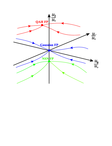
Figure 1: (Color online) Schematic flows of fermion-fermion couplings influenced by the interplay of fermion-fermion interactions and impurity scatterings with designating $u_{+}\equiv\frac{1}{2}(u_{3}+u_{1})$ and $u_{-}\equiv\frac{1}{2}(u_{3}-u_{1})$. There are three distinct types of FPs at the lowest-energy limit, namely Gaussian FP $(u_{0},u_{-},u_{2})/u_{+}\rightarrow(0,0,0)$, QAH FP $(u_{0},u_{-},u_{2})/u_{+}\rightarrow(0,-3.73,7.46)$, and NSN FP $(u_{0},u_{-},u_{2})/u_{+}\rightarrow(0,0,-1.09)$ at the weak impurity Wang2017PRB .

IV Stability of QBCP’s dispersion

Reading from Eqs. (14)-(16), one can directly realize that the parameters $t_{0}$, $t_{1}$, and $t_{3}$, which are closely related to the structure of the QBCP system, are energy-independent constants in the clean limit. In sharp contrast, the parameters $t_{0,1,3}$ are no longer constants but intimately hinge upon the evolutions of other interaction parameters directly or indirectly after taking into account the effects of impurity scatterings. This implies that the stability of QBCP’s dispersion would be challenged by the effects of impurities with the variation of energy scale. As the low-energy phenomena are closely associated with its stability, it is therefore imperative to examine whether QBCP’s dispersion is still robust and how it is changed under the influences of fermion-fermion interactions and impurities. To this end, we adopt the RG method together with the criterion $|t_{0}|<\mathrm{min}(|t_{1}|,|t_{3}|)$ to judge the stability of band structure in the whole energy region ranging from the starting point to the lowest-energy limit. Given our approach is based on the combination of definition of QBCP band structure and RG analysis, we can not only track the stability of the QBCP band structure in the whole energy region but also work effectively for both topological trivial and non-trivial phase transitions Fradkin2009PRL ; Murray2014PRB ; Wang2017PRB .

IV.1 Distinct sorts of fixed points

Before going further, we would like to stress that the fermion-fermion interactions can flow towards strong couplings after taking into account one-loop corrections. With this respect, we rescale all the interaction parameters by a combination of two non-sign changed couplings to overcome the strong couplings and make our study perturbative Murray2014PRB . Consequently, we are left with relative evolutions of interaction parameters together with the corresponding relatively fixed points (FPs) in the parameter space, which are the Gaussian, quantum anomalous Hall (QAH), and nematic-spin-nematic (NSN) on sites of bonds, respectively Murray2014PRB ; Wang2017PRB .

Considering the low-energy phenomena are conventionally dictated by these fixed points, it is therefore necessary to put our focus on monitoring the physical behaviors upon accessing these different fixed points. Given the Gaussian FP is relatively trivial, we hereby address brief comments on the QAH and NSN FPs. Generally, the QAH and NSN FPs in the presence of fermion-fermion interactions and impurities correspond to $(u_{0},u_{-},u_{2})/u_{+}=(0,a,b)$ and $(u_{0},u_{-},u_{2})/u_{+}=(0,0,c)$, respectively Murray2014PRB ; Wang2017PRB . Here, $a$, $b$, and $c$ are finite constants, which are dependent mildly upon the initial conditions. However, it is worth highlighting that the instabilities around these two fixed points are considerably robust although the specific values of $a,b,c$ can be slightly modified by tuning the starting values of impurity scatterings Murray2014PRB ; Wang2017PRB . In other words, the phase transitions induced nearby these two FPs are still from QBCP materials to the QAH and NSN states against the variations of these three constants. For instance, these FPs in the weak impurity respectively flow to Gaussian FP $(u_{0},u_{-},u_{2})/u_{+}=(0,0,0)$ and QAH FP $(u_{0},u_{-},u_{2})=(0,-3.73,7.46)u_{+}$ as well as NSN FP $(u_{0},u_{-},u_{2})=(0,0,-1.09)u_{+}$. Considering the impurity scatterings only slightly alter the concrete values but do not change the basic structures and features of these FPs, we provide a schematic evolutions absorbed by these potential FPs in the weak impurity as shown in Fig. 1.

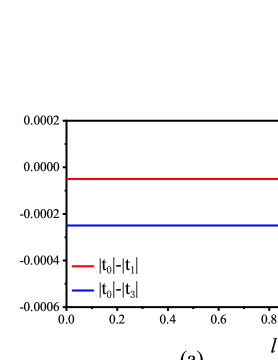
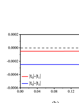
Figure 2: (Color online) Evolutions of $|t_{0}|-|t_{1}|$ and $|t_{0}|-|t_{3}|$ once the fermion-fermion interactions are driven to the Gaussian FP under (a) the sole presence of $M_{0}=\sigma_{0}$ impurity with $v_{i}(0)=10^{-3}$ (the results for $M_{1,2,3}$ are similar and hence not shown here) and (b) the presence of all three types of impurities with $v_{i}(0)=10^{-4}$ for $t_{0}(0)>0,t_{1}(0)>0,t_{3}(0)>0$.

Combining the coupled RG equations with Fig. 1, we notice that the fermion-fermion interaction parameters exhibit distinct energy-dependent behaviors around these FPs, which give rise to distinct corrections to the evolutions of impurity strengths. As a result, the parameters $t_{0}$, $t_{1}$, and $t_{3}$ that are directly related to the flows of impurities (14)-(16) would receive very distinct contributions once the systems are approaching different types of FPs. Without lose of generalities, we will select some typical starting values of fermion-fermion interactions that can drive $u_{i}$ into these FPs and investigate the related physical properties one by one.

IV.2 Gaussian FP

At the outset, we consider the Gaussian FP. We firstly assume there exists only one type of impurity in the QBCP system. To simplify our analysis, we from now on let $\Delta_{i}=1$ as mentioned at the end of Sec. III and utilize the parameter $v_{i}$ with $i=0,1,2,3$ to measure the corresponding strength of fermion-impurity interaction. After carrying out the numerical evaluations of Eqs. (14)-(24), we find that $|t_{0}|-|t_{1}|<0$ and $|t_{0}|-|t_{3}|<0$ are always satisfied even the initial value of the impurity strength is adequately strong. Since the results for sole presence of $M_{i}$ impurity with $i=0,1,2,3$ are analogous, we here only provide the results for presence of $M_{0}$ as clearly delineated in Fig. 2(a). Then, we move to the general situation for the presence of all types of quenched impurities in the QBCP system. Paralleling similar procedures of $M_{0}$ impurity brings out qualitatively analogous corrections to parameters $t_{0}$, $t_{1}$, and $t_{3}$ as manifested in Fig. 2(b). Specifically, $|t_{0}|<\mathrm{min}(|t_{1}|,|t_{3}|)$ cannot be destroyed in the low-energy regime and hence the QBCP’s dispersion is stable against impurities. In addition, one can check that the relationship among $t_{0}$, $t_{1}$ and $t_{3}$ does not change significantly even though the impurity strength is increased. In other words, QBCP’ dispersion is stable regardless of strong or weak impurity around the Gaussian FP. It is hereby necessary to stress that we within this project employ the impurity scattering rate $\Gamma^{-1}_{i}\sim\Delta_{i}v^{2}_{i}/t_{0}$ (with $i=0,1,2,3$) Wang2017PRB measured by $\Lambda_{0}$ to distinguish the weak and strong impurities. Since the fermion-fermion interactions and fermion-impurity scatterings are considered on the same footing under the RG analysis, it is of particular significance to pay attention to the starting point at $l=0$. To be concrete, we regard it as the “weak” impurity once the effect of impurity is less important than that of fermion-fermion interaction, i.e., $\Gamma^{-1}_{i}(l=0)\ll u_{i}(l=0)$. On the contrary, it corresponds to the “strong” impurity if the influence of the impurity is comparable to fermion-fermion interaction’s with $\Gamma^{-1}_{i}(l=0)\sim u_{i}(l=0)$.

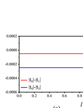
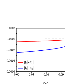
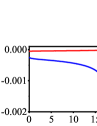
Figure 3: (Color online) Evolutions of $|t_{0}|-|t_{1}|$ and $|t_{0}|-|t_{3}|$ for the presence of $M_{0}=\sigma_{0}$ impurity as the fermion-fermion interactions are driven to the QAH/NSN FP with (a) a weak initial strength of $v_{i}(0)=10^{-5}$ and (b) a strong initial strength of $v_{i}(0)=10^{-3}$ (the results for $M_{1}$ and $M_{3}$ are similar and hence not shown here). Inset: flows for the presence of $M_{2}=\sigma_{2}$ impurity with a strong initial strength of $v_{i}(0)=10^{-3}$.

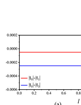
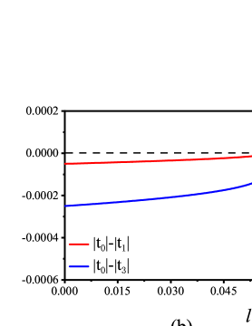
Figure 4: (Color online) Evolutions of $|t_{0}|-|t_{1}|$ and $|t_{0}|-|t_{3}|$ in the presence of all three types of impurities while the fermion-fermion interactions are driven to the QAH/NSN FP with (a) a weak initial strength of $v_{i}(0)=10^{-5}$ and (b) a strong initial strength of $v_{i}(0)=10^{-3}$.

IV.3 QAH and NSN FPs

Subsequently, we move to the case at which fermion-fermion interaction parameters are attracted and governed by QAH or NSN FP. To proceed, it is necessary to take into account the coupled evolutions on the same footing and carry out long but straightforward RG analysis.

Let us take QAH FP for an example. Again, we begin with visiting the effects caused by the presence of a single type of impurity and then consider the presence of all sorts of impurities. For instance, Fig. 3 manifestly exhibits how $|t_{0}|-|t_{1}|$ and $|t_{0}|-|t_{3}|$ evolve with lowering energy scales for the presence of impurity $M_{0}$ (the conclusions for the presence of $M_{1}$ or $M_{3}$ are qualitatively analogous and hence not shown here). One can readily find from Fig. 3(a) that the QBCP’s dispersion is robust at weak impurity. In comparison, we find the impurity scattering becomes more significant while the impurity strength is strong. To be concrete, $M_{0}$, $M_{1}$, or $M_{3}$ with sufficient impurity strength can trigger the divergence of $u_{i}$, indicating emergence of some impurity-induced FP at certain critical energy scale $l_{c}$, at which $|t_{0}|-|t_{1}|$ is converted into a positive value as delineated in Fig. 3(b). This suggests that QBCP’s dispersion is broken at $l_{c}$ and henceforth the RG evolutions should be stopped before this critical energy scale. However, as illustrated in the inset of Fig. 3(b), the restrictions $|t_{0}|-|t_{1}|<0$ and $|t_{0}|-|t_{3}|<0$ are always satisfied if only $M_{2}$ impurity is turned on even at the strong impurity strength. In other words, QBCP’s dispersion is rather stable for the sole presence of $M_{2}$ impurity around the QAH FP. While all three types of quenched impurities are present, we find that basic results as shown in Fig. 4 are consistent with the sole presence of $M_{0}$, $M_{1}$, or $M_{3}$. Nevertheless, it is necessary to address the following two points on the basis of Fig. 3 and Fig. 4. On one hand, impurity $M_{2}$ provides the contrary contribution compared to the other types of impurities, indicating the impurities $M_{0},M_{1},M_{3}$ are dominant over the $M_{2}$ impurity. On the other, we realize that the critical energy scale denoted by $l_{c}$ is slightly lifted, attesting to the competition among all kinds of impurity scatterings.

Additionally, one can check the basic results for NSN FP are similar to their QAH counterparts. Based on these points, we address that the relationship among $t_{0}$, $t_{1}$, and $t_{3}$, which is closely associated with the 2D QBCP’s dispersion, can either be robust or qualitatively changed by the interplay between fermionic interactions and impurities. Table 1 summarizes the stability of 2D QBCP’s dispersion against distinct types of impurities around different FPs. Before closing this section, it is interesting to point out that the parameters $t_{0,1,3}$ in principle can also be taken some negative values. As a result, there are in all eight types of starting values. We have checked that the above results are insusceptible to the signs of $t_{0,1,3}$. With these respects, we hereafter only consider the $t_{0,1,3}>0$ case.

Table 1: Fates of 2D QBCP’s dispersions under the influence of various impurities around the Gaussian, QAH, and NSN FPs. To be convenient, “$\mathcal{W}$” and “$\mathcal{S}$” are adopted to characterize weak and strong strengths of impurities. In addition, “$\mathbb{S}$” and “$\mathbb{US}$” stand for stable and unstable dispersions of 2D QBCP system, respectively.

$M_{0}$ $M_{1}$ $M_{2}$ $M_{3}$ $M_{0123}$ Strength $\mathcal{W}$ $\mathcal{S}$ $\mathcal{W}$ $\mathcal{S}$ $\mathcal{W}$ $\mathcal{S}$ $\mathcal{W}$ $\mathcal{S}$ $\mathcal{W}$ $\mathcal{S}$ Gaussian $\mathbb{S}$ $\mathbb{S}$ $\mathbb{S}$ $\mathbb{S}$ $\mathbb{S}$ $\mathbb{S}$ $\mathbb{S}$ $\mathbb{S}$ $\mathbb{S}$ $\mathbb{S}$ QAH/NSN $\mathbb{S}$ $\mathbb{US}$ $\mathbb{S}$ $\mathbb{US}$ $\mathbb{S}$ $\mathbb{S}$ $\mathbb{S}$ $\mathbb{US}$ $\mathbb{S}$ $\mathbb{US}$

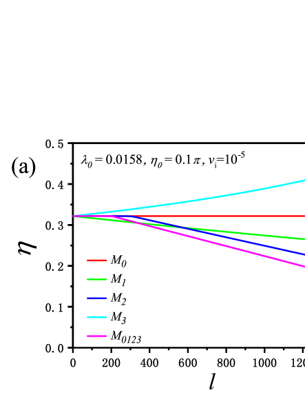
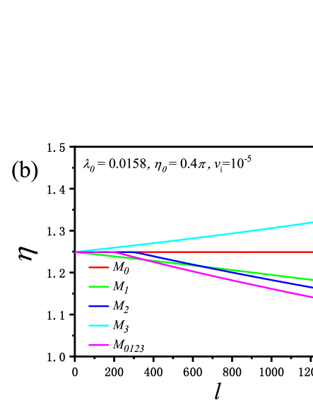
Figure 5: (Color online) Evolutions of $\eta$ against the presence of impurities at $v_{i}(0)=10^{-5}$ for (a) $\eta_{0}=0.1\pi$ and (b) $\eta_{0}=0.4\pi$ with fermion-fermion couplings flowing toward Gaussian FP.

V Fate of rotational asymmetry

As mentioned in Sec. II, rotational and particle-hole asymmetries are two quantities of remarkable importance for 2D QBCP systems, which are closely linked to the low-energy properties. To proceed, we follow Ref. Murray2014PRB and introduce two parameters $\eta$ and $\lambda$ to account for them,

$$\eta(l) \equiv \mathrm{arctan}\frac{t_{1}(l)}{t_{3}(l)},$$ (25)

$$\lambda(l) \equiv \frac{t_{0}(l)}{\sqrt{t^{2}_{1}(l)+t^{2}_{3}(l)}},$$ (26)

where $l$ serves as the energy scale and the related coefficients $t_{i}(l)$ with $i=0,1,3$ are designated in equations (14)-(16), which capture the information of rotational and particle-hole asymmetries (or symmetries) in 2D QBCP systems. As aforementioned, the 2D QBCP system would be invariant under rotational symmetry and/or particle-hole symmetry exactly at $\eta=\frac{\pi}{4}$ and/or $\lambda=0$. However, the parameters $t_{0}$, $t_{1}$, and $t_{3}$ are intimately intertwined with other interaction parameters obeying the coupled flow equations. A significant question is thus naturally raised whether and how $\eta$ and $\lambda$ are affected by the competition between fermion-fermion interactions and impurity scatterings.

Prior to responding to the above question, it is necessary to present some comments on the clean-limit situation. Via taking $v_{i}=0$ with $i=0-3$ in Eqs. (14)-(16), we can apparently reach that the parameters $t_{0}$, $t_{1}$, and $t_{3}$ are energy-independent and thus remain some constants at clean limit. As a consequence, the parameters of asymmetries (symmetries) $\eta$ and $\lambda$ are invariant with lowering the energy scale in the presence of fermion-fermion interactions. However, it is well-trodden that the impurities are always present in realistic systems and play an important role in determining the low-energy behaviors of fermionic systems Lee1985RMP ; Evers2008RMP ; Nersesyan1995NPB ; Hung2016PRB ; Efremov2011PRB ; Efremov2013NJP ; Korshunov2014PRB . In sharp distinction to a clean limit, the parameters $t_{0}$, $t_{1}$, and $t_{3}$ are no longer constants but intimately evolve and entangle with other interaction parameters due to the interplay between fermion-fermion interactions and impurities as clearly delineated in Eqs. (14)-(24). Under these respects, it is therefore of remarkable temptation to explore the energy-dependent hierarchies of parameters $\eta$ and $\lambda$, whose fates are closely associated with physical behaviors in the low-energy regime.

Learning from the coupled RG equations (14)-(24), one can readily realize that $\eta$ and $\lambda$ are manifestly affected by impurities. In comparison, the fermion-fermion interactions can indirectly impact $\eta$ and $\lambda$ by modifying the flows of $v_{i}$ with $i=0-3$. This signals that asymmetric parameters are in close conjunction with the evolutions of fermion-fermion interactions $u_{i}$ with $i=0-3$. As studied previously Murray2014PRB ; Wang2017PRB , it is worth pointing out that the fermion-fermion strengths $u_{i}$ in 2D QBCP systems are governed by the Gaussian, QAH, and NSN FPs induced by the impurity scatterings as schematically depicted in Fig. 1. Clearly, the energy-dependent $u_{i}$ would display considerably distinct trajectories in the vicinity of different types of FPs. This straightforwardly implies that different evolutions of $u_{i}(l)$ can bring inequivalent corrections to $\eta$ and $\lambda$. With these respects, we will separately investigate the effects of impurities and fermion-fermion interactions on $\eta$ and $\lambda$ as fermion-fermion strengths are attracted by Gaussian, QAH, and NSN FPs one by one.

Within this section, we put our focus on the low-energy behaviors of rotational asymmetry under the influence of both fermion-fermion interactions and impurities. The evolutions of particle-hole asymmetry will be left for Sec. VI. Since the QBCP’s dispersion is stable only in the region of $l<l_{c}$ as studied in Sec. IV, we hereafter confine this work within this energy regime.

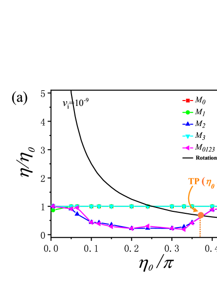
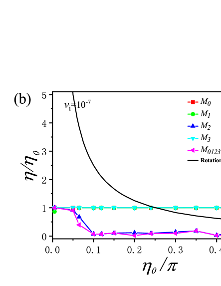
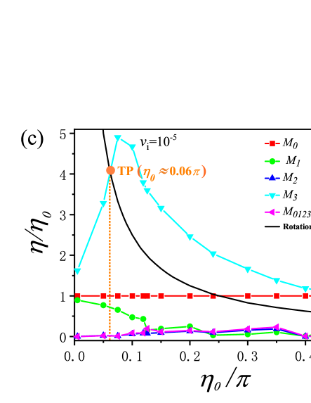
Figure 6: (Color online) Behaviors of $\eta(l\rightarrow l_{c})/\eta_{0}$ with tuning initial values of $\eta_{0}$ against the impurities for (a) $v_{i}(0)=10^{-9}$, (b) $v_{i}(0)=10^{-7}$, and (c) $v_{i}(0)=10^{-5}$ as the fermion-fermion couplings go towards Gaussian FP. The lines for the $M_{0}$ impurity coincide with their counterparts at clean limit and “TP” represents the very transition point from rotational asymmetry to symmetry.

V.1 Warm-up: Tendency of $\eta$ under impurities

As a warm-up, we hereby randomly choose several initial values for our interaction parameters and roughly check the tendency of $\eta$ under the presence of impurities. With these starting values, the energy-dependent evolutions of $\eta$ under the influence of distinct types of impurities are designated in Fig. 5 after performing the numerical analysis of RG equations (14)-(24). Reading off the information of Fig. 5, one can straightforwardly figure out that $\eta$ is insensitive to the sole presence of $M_{0}$ impurity. It is of particular interest to highlight that this result is well coincident with the analytical analysis. To be specific, the energy-dependent flow of $\eta$ can be specified as

$$\frac{dt_{1}/t_{3}}{dl} = \frac{1}{t_{3}}\frac{dt_{1}}{dl}-\frac{t_{1}}{t^{2}_{3}}\frac{dt_{3}}{dl}=\frac{t_{1}}{t_{3}}\left[(\Delta_{3}v^{2}_{3}-\Delta_{1}v^{2}_{1})\mathcal{N}_{6}\right.$$ (27)

$$- \left.(\Delta_{1}v^{2}_{1}+2\Delta_{2}v^{2}_{2}+\Delta_{3}v^{2}_{3})\mathcal{N}_{5}\right],$$

where the coefficients $\mathcal{N}_{5}$ and $\mathcal{N}_{6}$ are designated in Eq (51). Combining Eq (25) and Eq (27), one can readily draw a conclusion that the strength of $M_{0}$ impurity does not enter into the evolution and henceforth $\eta$ is independent of $M_{0}$. However, the value of $t_{1}/t_{3}$ appearing in Eq. (27) is closely related to other types of impurities. Accordingly, we only need to study the effects of $M_{1,2,3}$ impurities on the parameter $\eta$. To be concrete, the sole presence of $M_{1}$ or $M_{2}$ impurity causes $\eta$ to decrease with lowering the energy scale. In comparison, $\eta$ would be gradually increased with the reduction of energy scale once there exists the $M_{3}$ impurity in a 2D QBCP system. Moreover, as clearly depicted in Fig. 5, $\eta$ is apparently diminished under the influence of all types of impurities. As a result, it indicates the combination of $M_{1}$ and $M_{2}$ dominates over $M_{3}$ in the low-energy region.

V.2 Gaussian FP

Before going further, it is necessary to emphasize that the results of Fig. 5 (a) and (b) are based upon two concrete values, i.e., $\eta_{0}=0.1\pi$ and $\eta_{0}=0.4\pi$, respectively. However, we would like to point out the rotational parameter $\eta$ that is associated with the parameters $t_{1}$ and $t_{3}$ via $\eta=\mathrm{arctan}\frac{t_{1}}{t_{3}}$, in principle, can run through the following range $\eta\in\{[-\frac{\pi}{2},0)\cup(0,\frac{\pi}{2}]\}$ while the parameters $t_{0}$, $t_{1}$ and $t_{3}$ are restricted by $|t_{0}|<\mathrm{min}(|t_{1}|,|t_{3}|)$. At this stage, it therefore naturally raises a question of where the $\eta$ eventually goes toward at the lowest-energy limit once its initial value is randomly taken from this restricted range.

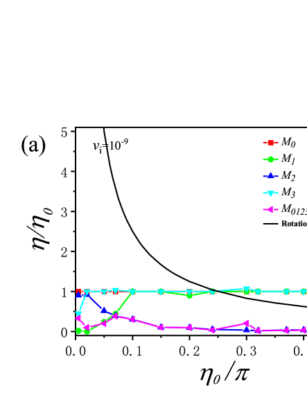
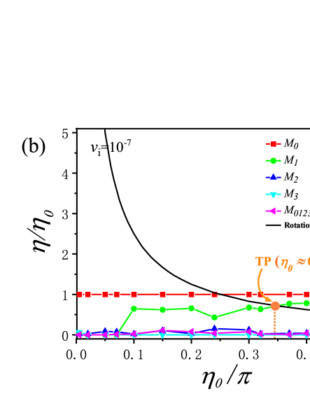
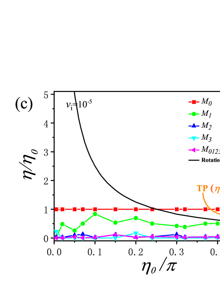
Figure 7: (Color online) Behaviors of $\eta(l\rightarrow l_{c})/\eta_{0}$ with varying initial values of $\eta_{0}$ against the impurities for (a) $v_{i}(0)=10^{-9}$, (b) $v_{i}(0)=10^{-7}$, and (c) $v_{i}(0)=10^{-5}$ as the fermion-fermion couplings flow towards the QAH FP. The lines for the $M_{0}$ impurity coincide with their counterparts at clean limit and “TP” represents the very transition point from rotational asymmetry to symmetry.

Without loss of generality, we only consider the right range with $\eta_{0}>0$ (the left range can be studied similarly) and then choose several representative starting values of $\eta$, impurity strengths, and fermion-fermion couplings that can drive the system into Gaussian FP. To proceed, the values of $\eta$ around the Gaussian FP can be extracted from the coupled RG equations that involve the competitions between fermion-fermion interactions and impurity scatterings in the proximity of critical energy scale. Fig. 6 collects our primary results for $\eta$. At the first sight, we find that $M_{1}$ impurity just brings about slight impacts on $\eta$ when its strength is very weak as shown in Fig. 6(a) and Fig. 6(b). Whereas the values of $\eta$ are pulled down once the $M_{1}$ impurity strength is sufficiently enhanced as clearly displayed in Fig. 6(c). Although the parameter $\eta$ does not receive any corrections at weak $M_{3}$ impurity, it is worth highlighting that $M_{3}$, as opposed to the $M_{1}$ impurity, is in favor of increasing $\eta$ in the entire region if the initial impurity strength is strong, such as $v_{i}=10^{-5}$ in Fig. 6(c). Subsequently, we move to study the changes of $\eta$ due to the single presence of $M_{2}$ impurity. The blue curves in Fig 6 apparently indicate that the value of $\eta$ is sensitive to the impurity strength, which is heavily reduced by the $M_{2}$ impurity and even driven to zero at the strong impurity strength. Furthermore, one can find with the help of Fig. 6 that $M_{2}$ impurity plays a leading role among other types of impurities once all three types of impurities are present in the 2D QBCP system. Consequently, the basic results are analogous to the sole presence of $M_{2}$ impurity. Besides, the parameter $\eta$ is also slightly dependent upon its initial value. The second line of Table 2 briefly lists the effects of various types of impurities on the rotational parameter $\eta$.

As aforementioned, the symmetry parameter $\eta$ of 2D QBCP system is proved to be energy-independent at clean limit. However, Fig. 5 indicates that impurities would bring considerable influence to this physical quantity. On one side, the parameter $\eta$ can be robustly protected against sole $M_{0}$ impurity. On the other, it would be either increased or decreased under the presence of other types of impurities. Under such circumstances, it is of considerable interest to ask how these impurities affect the rotational asymmetry of 2D QBCP system and whether the rotational symmetry can be induced from asymmetry case.

To facilitate our discussions, we provide the black curves in Fig. 6 to show the situations that harbor rotational symmetry. In addition, since the $M_{0}$ impurity does not influence $\eta$ at all, we hereby consider the red lines as the clean-limit cases for convenient comparisons. With the help of these two kinds of curves, we find that the space between parameter $\eta$ and black line is susceptible to $M_{1}$, $M_{2}$, or $M_{3}$ impurity compared to clean limit. As a result, it is of particular interest to point out that the transition from rotational asymmetry to rotational symmetry can be triggered by some weak $M_{2}$ impurity or strong $M_{3}$ impurity at certain $\eta_{0}$, which are denoted by the intersections dubbed transition point (TP) in Fig. 6 (a) and (c). However, we would like to stress that the condition for impurity-induced rotational symmetry is remarkably strict and in principle the presence of impurities in the 2D QBCP system is detrimental to the rotational symmetry in the case of $u_{i}(0)$ flowing towards Gaussian FP. In other words, the recovery of rotational symmetry from asymmetry is only a specific inference (or an intriguing ingredient) of our primary results.

V.3 QAH FP

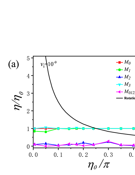
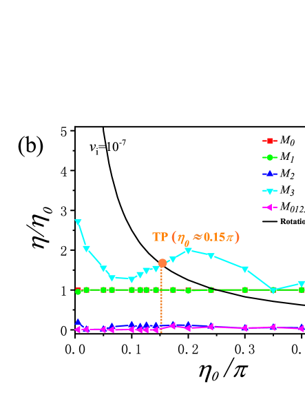
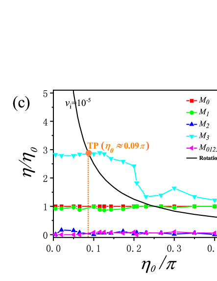
Figure 8: (Color online) Behaviors of $\eta(l\rightarrow l_{c})/\eta_{0}$ with varying initial values of $\eta_{0}$ against the impurities for (a) $v_{i}(0)=10^{-9}$, (b) $v_{i}(0)=10^{-7}$, and (c) $v_{i}(0)=10^{-5}$ as the fermion-fermion couplings flow towards the NSN FP. The lines for the $M_{0}$ impurity coincide with their counterparts at clean limit and “TP” represents the very transition point from rotational asymmetry to symmetry.

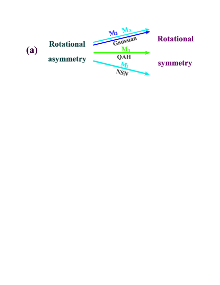
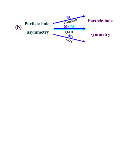
Figure 9: (Color online) Potential transitions (a) from rotational asymmetry to rotational symmetry and (b) from particle-hole asymmetry to particle-hole symmetry under certain type of impurity as the fermion-fermion interactions are driven to distinct sorts of FPs.

Subsequently, we turn to study how the parameter $\eta$ behaves against the impurities while the fermion-fermion interactions are governed by the QAH FP with certain starting values of $u_{i}(0)$. Fig. 7 collects our primary results of $\eta$ caused by impurities at the lowest-energy limit after performing the numerical evolution. Again, the black curves correspond to the situations with rotational symmetry and the red lines stand for clean-limit cases.

At first, we find that the rotational parameter $\eta$ is stable under the weak $M_{1}$ impurity but would be decreased in the low-energy regime as long as the impurity strength is sufficiently strong. This is similar to its Gaussian counterpart. Besides, it is of particular interest to address that the subtle combination of $M_{1}$ impurity and fermion-fermion interaction is endowed with a potential ability to drive an anisotropic system into an isotropic one with the rotational symmetry at certain very $\eta_{0}$. These unique positions denoted by TP at which the phase transitions set in are illustrated in Fig. 7 (b) and (c). Next, we inspect the behaviors of $\eta$ under the influence of only $M_{2}$ impurity. Fig. 7 singles out that $\eta$ is quickly diminished and departs from the symmetric curve with tuning up $v_{i}$. This implies that it is difficult under $M_{2}$ impurity to achieve rotational symmetry from anisotropic case in the 2D QBCP system. Similarly, comparing the blue lines of Fig. 6 with Fig. 7, we find that the values of $\eta$ at QAH FP are reduced and deviated more from rotational symmetry’s than their Gaussian counterparts especially in the presence of weak impurity. This indicates that $u_{i}$ flowing towards QAH FP is more detrimental to the rotational symmetry. As a result, competition between fermion-fermion interaction and $M_{2}$ impurity is sensitive to the FP. Moreover, as opposed to the Gaussian situation, the parameter $\eta$ depicted in Fig. 7 (b) and (c) would be reduced or even go towards zero with lowering the energy scale in the presence of the sole $M_{3}$ impurity. Different trajectories of fermion-fermion interactions for QAH and Gaussian FPs may be responsible for these distinctions. In other words, fermion-fermion interactions win against the $M_{3}$ impurity while the fermionic couplings are approaching to QAH FP and thus cause the original contribution of $M_{3}$ impurity to be neutralized. At last, we realize that the fates of parameter $\eta$ are similar to the sole presence of $M_{2}$ or $M_{3}$ impurity once there exist all three different types of impurities in 2D QBCP system. To recapitulate, the presence of impurity is conventionally harmful to the formation of rotational symmetry except the very point under the $M_{1}$ impurity at which the rotational symmetry is preferred.

V.4 NSN FP

At last, we go to the case with fermion-fermion interactions evolving towards NSN FP. In order to unveil the fate of the rotational parameter $\eta$ in the vicinity of NSN FP, we parallel several tedious but straightforward calculations that are similar to the procedures for QAH FP and then present our main results in Fig. 8 from which one can figure out that the effects of various impurities on $\eta$ are sensitive to the initial values of $\eta(0)$.

Table 2: Qualitative effects of different types of impurities on the rotational parameter $\eta$ at $v_{i}(0)=10^{-5}$ approaching distinct sorts of FPs. Hereby, “–” indicates $\eta$ is hardly influenced or remains certain constant. Instead, “$\uparrow$” and “$\downarrow$” stand for the increase and decrease with lowering the energy scale, respectively (the double arrows indicate much more increase or decrease).

$M_{0}$ $M_{1}$ $M_{2}$ $M_{3}$ $M_{0123}$ Gaussian FP – $\downarrow$ $\downarrow\downarrow$ $\uparrow$ $\downarrow\downarrow$ QAH FP – $\downarrow$ $\downarrow\downarrow$ $\downarrow\downarrow$ $\downarrow\downarrow$ NSN FP – – $\downarrow\downarrow$ $\uparrow$ $\downarrow\downarrow$

At the outset, we find that the contributions of $M_{0}$ or $M_{1}$ impurity to the parameter $\eta$ are negligible even at strong impurity with lowering the energy scale. This suggests that both of them prefer to protect the stability of $\eta$ nearby NSN FP. Then, we turn to examine the effect of the sole presence of $M_{2}$ impurity. Studying from Fig. 8, one can readily realize that the $M_{2}$ impurity plays a significant role in pinning down the low-energy fate of parameter $\eta$ around the NSN FP. Apparently, $\eta$ is heavily reduced with lowering the energy scale. As a consequence, the $M_{2}$ impurity is considerably detrimental to the rotational symmetry around NSF FP in 2D QBCP system. Compared to the Gaussian case, its effects are more manifest and powerful. This may be ascribed to the intimate coupling between $M_{2}$ impurity and the fermion-fermion interactions accessing the NSN FP. Besides the $M_{0,1,2}$ impurities, several intriguing results are also generated by the sole presence of $M_{3}$ impurity. In distinction to other sorts of impurities, the $M_{3}$ impurity is prone to increase the value of $\eta$ once its initial strength is suitable, as apparently exhibited by cyan lines of Fig. 8. Analogous to the unique phenomena sparked by $M_{1}$ around QAH FP and $M_{3}$ nearby Gaussian FP, Fig. 8(b) and (c) show that certain transition from rotational asymmetry to rotational symmetry can be triggered by the adequately strong $M_{3}$ impurity in the proximity of NSN FP. Furthermore, we briefly comment on the concomitant presence of all types of impurities in 2D QBCP system around NSN FP. Learning from Fig. 8, one readily figures out that the basic tendencies are consistent with the sole $M_{2}$ impurity; namely, $\eta$ is substantially decreased via lowering the energy scale. This corroborates again that the $M_{2}$ impurity takes a leading responsibility in governing the low-energy properties.

To be brief, the effects of impurities on the rotational parameter $\eta$ are very different while the fermion-fermion interactions are controlled by distinct sorts of FPs. Fig 9 (a) and Table 2 summarize our primary conclusions for the low-energy behaviors of parameter $\eta$ under the competitions between fermion-fermion interactions and impurities scatterings. Before closing this section, we would like to emphasize again that both closely energy and intimately starting-value dependence of low-energy fates of the asymmetric parameter $\eta$ constitute our primary conclusions. In comparison, the underlying transition from rotational to symmetric situation is only an interesting ingredient of our main results under certain restricted condition.

VI Fate of particle-hole asymmetry

In the previous section, we address the effects of competitions between fermion-fermion interactions and impurity scatterings on rotational asymmetry parameter $\eta$ while the fermion-fermion couplings $u_{i}$ are governed by three distinct types of FPs. To proceed, we within this section endeavor to investigate the behaviors of particle-hole asymmetry $\lambda$ under these three distinct situations.

VI.1 Warm-up and Gaussian FP

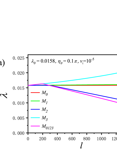
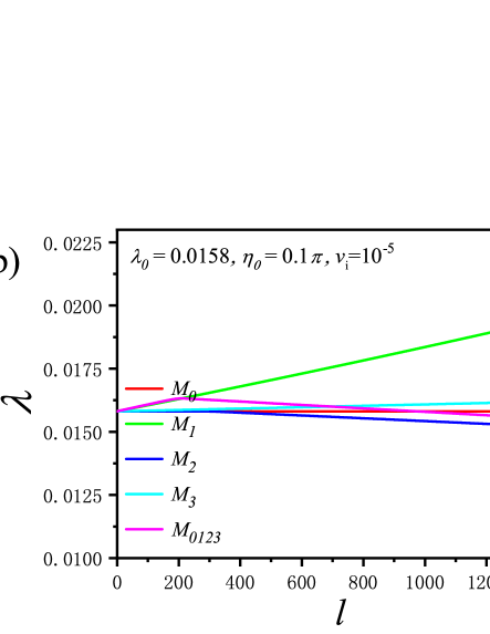
Figure 10: (Color online) Evolutions of $\lambda$ against the presence of impurities at $v_{i}(0)=10^{-5}$ for (a) $\eta_{0}=0.1\pi$ and (b) $\eta_{0}=0.4\pi$ with fermion-fermion couplings flowing towards Gaussian FP.

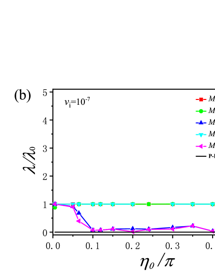
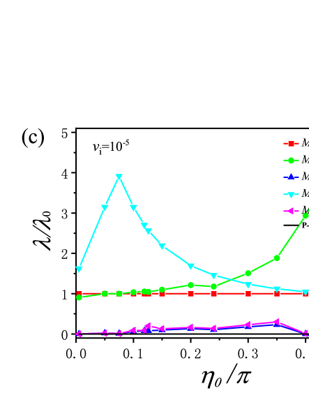
Figure 11: (Color online) Behaviors of $\lambda(l\!\!\longrightarrow\!\!l_{c})/\lambda_{0}$ with varying initial values of $\eta_{0}$ against the impurities for (a) $v_{i}(0)=10^{-9}$, (b) $v_{i}(0)=10^{-7}$, and (c) $v_{i}(0)=10^{-5}$ once the fermion-fermion interactions flow towards Gaussian FP. The lines for the $M_{0}$ impurity coincide with their counterparts at clean limit.

Before moving further, we would like to make a warm-up again to roughly check the energy-dependent tendency of the particle-hole parameter $\lambda$ in the presence of impurity. Without loss of generalities, we follow the steps of Sec. V.1 by choosing specific starting values for interaction parameters and show the influence of distinct types of impurities on the low-energy behaviors of parameter $\lambda$ in Fig. 10. Reading off Fig. 10, we realize that both impurities $M_{1}$ and $M_{3}$ prefer to increase the parameter $\lambda$ as the energy scale is lowered. On the contrary, it climbs down in the presence of sole $M_{2}$ or all three types of impurities.

Again, we would like to highlight that Fig. 10 only collects the energy-dependent information of parameter $\lambda$ at $\eta_{0}=0.1\pi$ and $\eta_{0}=0.4\pi$. As mentioned in Sec. V.2, the rotational parameter $\eta$ satisfies $\eta\in\{[-\frac{\pi}{2},0)\cup(0,\frac{\pi}{2}]\}$ once the QBCP’s dispersion is stable. In order to capture more physical information at the lowest-energy limit, it is necessary to sort out representative starting values of $\eta$ that are distributed in the whole restricted range.

Subsequently, we put our focus on the Gaussian FP. After carrying out the numerical studies with variation of the initial value of $\eta$, the principal results are summarized in Fig. 11, where red and black lines in consistent with Fig. 6 for the parameter $\eta$ are exploited to characterize the clean-limit case and 2D QBCP system with particle-hole symmetry, respectively. Specifically, Fig. 11(a) and (b) uncover that the low-energy values of $\frac{\lambda}{\lambda_{0}}$ at the weak impurities are almost unaffected against the presence of a sole $M_{1}$ or $M_{3}$ impurity. However, Fig. 11(c) shows that the parameter $\lambda$ largely climbs up once the impurity strengths are adequately strong. As a result, the $M_{1}$ or $M_{3}$ impurity is harmful to the particle-hole symmetry. In comparison, the $M_{2}$ impurity is prone to heavily reduce the parameter $\lambda$, which is forced to flow towards zero as the impurity is sufficiently increased. Moreover, when all types of impurities are present simultaneously, the $M_{1,3}$ and $M_{2}$ ferociously compete as their contributions are exactly converse. Eventually, as depicted in Fig. 11, $M_{2}$ wins the competition and hence the basic results are consistent with the sole presence of the $M_{2}$ impurity. In other words, this proposes that $M_{2}$ impurity, compared to other sorts of impurities, brings the major contribution to the parameter $\lambda$ in the low-energy regime. To proceed, we try to investigate whether these impurities are favorable for particle-hole symmetry around the Gaussian FP. Given the 2D QBCP system possesses the particle-hole symmetry exactly at $\lambda=0$, one, with the help of Fig. 11, can infer that the presence of the $M_{2}$ impurity alone or three different types of impurities indeed promote the particle-hole symmetry in 2D the QBCP system.

VI.2 QAH FP

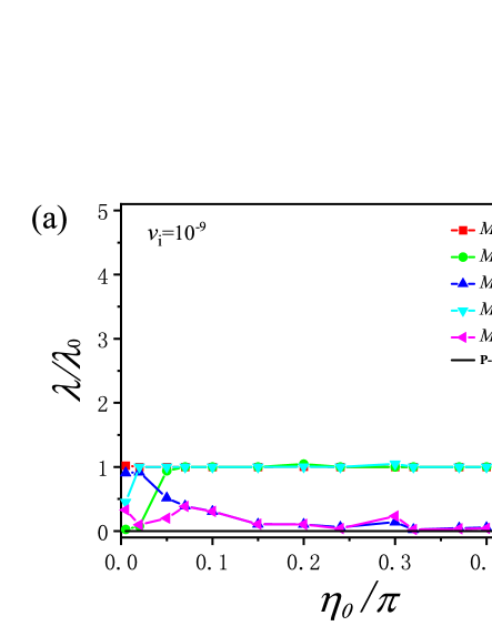
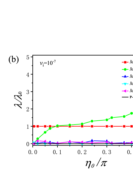
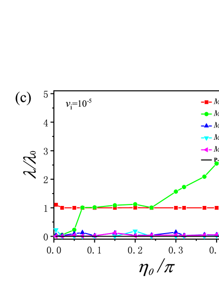
Figure 12: (Color online) Behaviors of $\lambda(l\!\!\longrightarrow\!\!l_{c})/\lambda_{0}$ with varying initial values of $\eta_{0}$ against the impurities for (a) $v_{i}(0)=10^{-9}$, (b) $v_{i}(0)=10^{-7}$, and (c) $v_{i}(0)=10^{-5}$ once the fermion-fermion interactions flow towards QAH FP. The lines for the $M_{0}$ impurity coincide with their counterparts at a clean limit.

Subsequently, we move our target to the situation at which the system is attracted by QAH FP. With the help of coupled RG equations (14)-(24) and repeating the procedures in Sec. VI.1, we are able to present the energy-dependent evolutions of particle-hole parameter $\lambda$, which carry the physical information about the competitions between impurities and fermion-fermion interactions.

Fig. 12 manifestly characterizes the physical key points for parameter $\lambda$ against impurities in the proximity of QAH FP. To be specific, we find from Fig. 12 that the red curves remain invariant and stable for the whole regime of parameter $\eta$. In other words, the parameter $\lambda$ is very insensitive to the $M_{0}$ impurity. Additionally, $\lambda$ exhibits manifestly $\eta_{0}$-dependent behaviors under the $M_{1}$ impurity. On one hand, the parameter $\lambda$ receives significant revision at $\eta_{0}<0.07\pi$, which is insusceptible to impurity strength. On the other, the effects of weak $M_{1}$ impurity on the parameter $\lambda$ are negligible at $\eta_{0}\geq 0.07\pi$ as depicted in Fig. 12(a). However, as the initial strength increases, the $M_{1}$ impurity can cause an enhancement of parameter $\lambda$ as shown in Fig. 12(b) and (c). In comparison, more interesting effects on $\lambda$ are triggered by the sole presence of $M_{2}$ impurity around the QAH FP. Fig. 12 apparently exhibits the parameter $\lambda$ is heavily reduced under the $M_{2}$ impurity. In particular, it almost vanishes while the $M_{2}$ impurity strength is adequate strong as clearly shown in Fig. 12(b) and (c). This indicates that the transformation from particle-hole asymmetry to symmetry would be expected in that the 2D QBCP system is invariant under the particle-hole transformation at $\lambda=0$. In other words, $M_{2}$ impurity is very much in favor of particle-hole symmetry. Furthermore, one can readily capture the information from Fig. 12 that the presence of all sorts of impurities shares the common basic conclusions with the sole type of $M_{2}$ impurity irrespective of impurity strength. This again corroborates the $M_{2}$ impurity dominates over other impurities. At last, we briefly address the effects of $M_{3}$ impurity scattering. The influence of weak $M_{3}$ impurity is consistent with its $M_{1}$ counterpart as depicted in Fig. 12(a). Rather, in analogy with the $M_{2}$ impurity illustrated in Fig. 12(b) and (c), it prefers to promote the particle-hole symmetry whilst the starting value is increased. Compared to the properties around Gaussian FP, these results unambiguously shed light on the importance of M3 impurity that behaves like a catalyst to ignite fermion-fermion interactions in boosting particle-hole symmetry as the system approaches the QAH FP.

VI.3 NSN FP

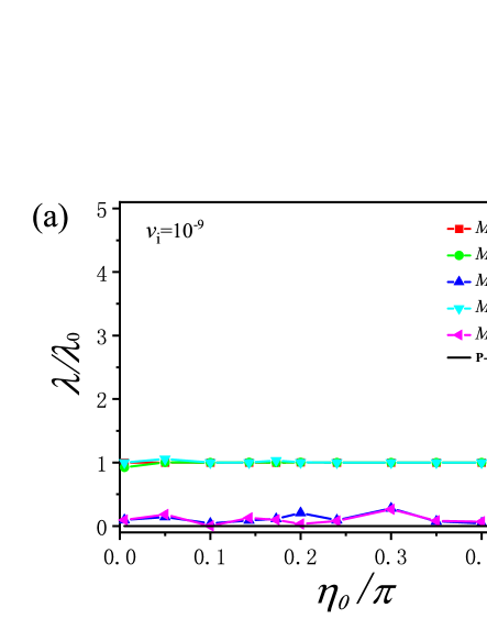
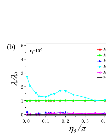
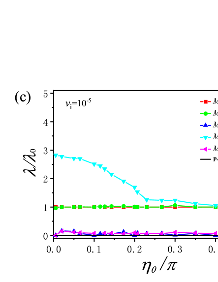
Figure 13: (Color online) Behaviors of $\lambda(l\!\!\longrightarrow\!\!l_{c})/\lambda_{0}$ with varying initial values of $\eta(0)$ against the impurities for (a) $v_{i}(0)=10^{-9}$, (b) $v_{i}(0)=10^{-7}$, and (c) $v_{i}(0)=10^{-5}$ once the fermion-fermion interactions flow towards the NSN FP. The lines for the $M_{0}$ impurity coincide with their counterparts at clean limit.

Finally, we turn to extract the low-energy fates of particle-hole parameter $\lambda$ from the coupled RG equations under distinct types of impurities in the proximity of NSN FP.

After carrying out tedious but straightforward calculations with variation of the initial values of $\eta$, the main results for the low-energy properties of $\frac{\lambda}{\lambda_{0}}$ are collected in Fig. 13. At the first sight, we get that the values of $\lambda$ at the critical energy denoted by $l_{c}$ are very stable if there only exists the sole $M_{0}$ or $M_{1}$ impurity in the 2D QBCP system. This indicates that the $M_{1}$ impurity accessing to the NSN FP plays a very distinct role in determining the fate of parameter $\lambda$ compared to other FPs studied in Sec. VI.1 and Sec. VI.2. Distinct energy-dependent trajectories of fermion-fermion couplings around three types of FPs may be responsible for this difference. With respect to the $M_{2}$ impurity, parameter $\lambda$ displays a sharp drop as shown in blue curves of Fig. 13. As mentioned for Gaussian and QAH FPs, this suggests that the transformation from particle-hole asymmetry to particle-hole symmetry can be manifestly realized in 2D QBCP system with the help of $M_{2}$ impurity. On the contrary, as to the $M_{3}$ impurity, it inclines to lift the parameter $\lambda$ and therefore hinders the particle-hole symmetry of the system once the impurity strength is sufficient strong. Furthermore, Fig. 13 distinctly shows that the impact of the presence of all types of impurities on $\lambda$ is in agreement with the sole presence of $M_{2}$ impurity. This again proves the leading role of $M_{2}$ impurity among all sorts of impurities.

To recapitulate, we within this section carefully investigate the influence of various sorts of impurities on the particle-hole asymmetry parameter $\lambda$ while the fermion-fermion couplings are governed by three distinct types of FPs. Several interesting results are obtained. For instance, certain type of impurity can induce very distinct effects on the parameter $\lambda$ in the vicinity of different types of FPs. In addition, the 2D QBCP system may undergo the transition from particle-hole asymmetry to symmetry in the restricted conditions. Concretely, $M_{2}$ impurity prefers to trigger the particle-hole symmetry at all three different types FPs, while $M_{3}$ can evoke the symmetry of system only at QAH FP. Fig 9 (b) and Table 3 summarize our primary conclusions for the low-energy behaviors of parameter $\lambda$ under the competitions between fermion-fermion interactions and impurity scatterings.

Table 3: Qualitative effects of different types of impurities on the particle-hole parameter $\lambda$ at $v_{i}(0)=10^{-5}$ approaching distinct sorts of FPs. Hereby, “–” indicates $\lambda$ is hardly influenced or remains certain constant. Instead, “$\uparrow$” and “$\downarrow$” stand for the increase and decrease with lowering the energy scale, respectively (the double arrows indicate much more increase or decrease).

$M_{0}$ $M_{1}$   $M_{2}$ $\hskip 5.69046ptM_{3}$ $\hskip 5.69046ptM_{0123}$ Gaussian FP – $\uparrow$ $\downarrow\downarrow$  $\uparrow$ $\downarrow\downarrow$       QAH FP – $\downarrow$  $\frac{\eta_{0}}{\pi}\in(0,0.07)$ $\downarrow\downarrow$ $\downarrow\downarrow$ $\downarrow\downarrow$ $\uparrow$  $\frac{\eta_{0}}{\pi}\in(0.07,0.5)$ NSN FP – – $\downarrow\downarrow$  $\uparrow$ $\downarrow\downarrow$

VII Summary

In summary, we study the effects of the competitions between fermion-fermion interactions and impurity scatterings on the low-energy stabilities of 2D asymmetric QBCP materials by virtue of the RG approach Shankar1994RMP ; Wilson1975RMP ; Polchinski9210046 . To be specific, we find that the band structure and dispersion of 2D QBCP systems are considerably robust irrespective of weak or strong impurities while fermion-fermion interactions flow toward the Gaussian FP. Rather, they can either be stable or collapsed if fermionc couplings are attracted by nontrivial QAH and NSN FPs. Table 1 briefly shows our main results for distinct kinds of FPs under distinct sorts of impurities. Additionally, the low-energy fates of rotational and particle-hole asymmetries that are characterized by $\eta$ and $\lambda$ are attentively investigated. With variations of initial values of fermion-fermion interactions and impurities, these two parameters exhibit intimately energy-dependent behaviors and can either be remarkably increased or heavily reduced. It is worth highlighting that the $M_{2}$ impurity plays the most important role among all impurities. Table 2 and Table 3 collect qualitative results for different sorts of impurities. In addition to these basic conclusions, we find that, under certain restricted condition in 2D QBCP systems, the transition from rotational asymmetry or particle-hole asymmetry to rotational symmetry or particle-hole symmetry can be induced by the interplay between fermion-fermion interactions and impurities.

Furthermore, we hereby present brief comments on symmetric studies Fradkin2009PRL ; Murray2014PRB and our asymmetric case. With respect to the former that is an ideal limit, the QBCP band structure is stable and both of two symmetries are robust as well as the energy dependence of physical implications are absent due to the trivial properties of structural parameters. In comparison, we consider a general asymmetric QBCP system and develop a suitable approach to judge whether the QBCP band structure is stable and track how the asymmetries behave in the whole energy region from a starting point to certain FP. Our results theoretically corroborate the QBCP band structure may be destroyed and asymmetric parameters can be heavily affected in the vicinity of FPs. Additionally, we guess that the energy-dependent behaviors of physical observables upon accessing a specific FP would be principally captured in the asymmetric situation by taking advantage of the coupled RG equations consisting of both structural and interaction parameters. These signal that monitoring the stability of band structure is imperative while one studies the latter case. To recapitulate, we expect our studies are instructive to provide helpful clues for enhancing the stability and exploring other singular behaviors of 2D QBCP systems.

Appendix A one-loop corrections

The one-loop corrections to self-energy, fermion-fermion couplings, and fermion-impurity vertexes are depicted in Fig. 14, Fig. 15 and Fig. 16, respectively. After long but straightforward calculations, we obtain

$$\delta\Sigma(\omega,\mathbf{k})\!\! = \!\!-\mathcal{N}_{1}(v^{2}_{0}\Delta_{0}+v^{2}_{1}\Delta_{1}+v^{2}_{2}\Delta_{2}+v^{2}_{3}\Delta_{3})(i\omega)+\mathcal{N}_{3}(v^{2}_{0}\Delta_{0}+v^{2}_{1}\Delta_{1}+v^{2}_{2}\Delta_{2}+v^{2}_{3}\Delta_{3})(t_{0}\mathbf{k}^{2})$$ (28)

$$\!\!-\!\mathcal{N}_{3}(v^{2}_{0}\Delta_{0}+v^{2}_{1}\Delta_{1}-v^{2}_{2}\Delta_{2}-v^{2}_{3}\Delta_{3})(2t_{1}k_{x}k_{y}\sigma_{1})\!\!-\!\!\mathcal{N}_{3}(v^{2}_{0}\Delta_{0}-v^{2}_{1}\Delta_{1}-v^{2}_{2}\Delta_{2}+v^{2}_{3}\Delta_{3})[t_{3}(k^{2}_{x}\!-\!k^{2}_{y})\sigma_{3}],$$

for one-loop corrections to self-energy derived from Fig. 14,

$$\delta\mathcal{S}_{u_{0}}\!\! = \!\!u_{0}\int^{+\infty}_{-\infty}\frac{d\omega_{1}d\omega_{2}d\omega_{3}}{(2\pi)^{3}}\int^{b}\frac{d^{2}\mathbf{k}_{1}d^{2}\mathbf{k}_{2}d^{2}\mathbf{k}_{3}}{(2\pi)^{6}}\psi^{\dagger}(\omega_{1},\mathbf{k}_{1})\sigma_{0}\psi(\omega_{2},\mathbf{k}_{2})\psi^{\dagger}(\omega_{3},\mathbf{k}_{3})\sigma_{0}\psi(\omega_{1}+\omega_{2}-\omega_{3},\mathbf{k}_{1}+\mathbf{k}_{2}-\mathbf{k}_{3})$$ (29)

$$\times\Bigl{\{}\frac{l}{8\pi u_{0}\sqrt{2(t^{2}_{1}+t^{2}_{3})}}\left[-\mathcal{C}_{1}(u^{2}_{0}+u^{2}_{1}+u^{2}_{2}+u^{2}_{3})-\mathcal{C}_{2}(u_{0}u_{1}+u_{2}u_{3})-\mathcal{C}_{3}(u_{0}u_{3}+u_{1}u_{2})\right.$$

$$\left.-\mathcal{C}_{4}(u_{0}u_{1}-u_{2}u_{3})-\mathcal{C}_{5}(u_{0}u_{3}-u_{1}u_{2})\right]+2\pi l\sqrt{2(t^{2}_{1}+t^{2}_{3})}\left[v^{2}_{0}\Delta_{0}(\mathcal{D}_{0}+2\mathcal{N}_{1})\right.$$

$$\left.+2v^{2}_{2}\Delta_{2}\mathcal{N}_{1}+v^{2}_{1}\Delta_{1}(\mathcal{D}_{1}+2\mathcal{N}_{1})+v^{2}_{3}\Delta_{3}(\mathcal{D}_{2}+2\mathcal{N}_{1})\right]\Bigl{\}},$$

$$\delta\mathcal{S}_{u_{1}}\!\! = \!\!\left(u_{1}\int^{+\infty}_{-\infty}\frac{d\omega_{1}d\omega_{2}d\omega_{3}}{(2\pi)^{3}}\int^{b}\frac{d^{2}\mathbf{k}_{1}d^{2}\mathbf{k}_{2}d^{2}\mathbf{k}_{3}}{(2\pi)^{6}}\psi^{\dagger}(\omega_{1},\mathbf{k}_{1})\sigma_{1}\psi(\omega_{2},\mathbf{k}_{2})\psi^{\dagger}(\omega_{3},\mathbf{k}_{3})\sigma_{1}\psi(\omega_{1}+\omega_{2}-\omega_{3},\mathbf{k}_{1}+\mathbf{k}_{2}-\mathbf{k}_{3})\right)$$ (30)

$$\times\Bigl{\{}\frac{l}{4\pi u_{1}\sqrt{2(t^{2}_{1}+t^{2}_{3})}}\Bigl{[}(2u_{0}u_{1}-2u^{2}_{1}-2u_{2}u_{1}-3u_{3}u_{1}-u_{0}u_{2})\mathcal{C}_{3}+(u_{0}u_{1}+u_{2}u_{3})(\mathcal{C}_{2}+\mathcal{C}_{3})$$

$$-\frac{1}{2}(u^{2}_{0}+u^{2}_{1}+u^{2}_{2}+u^{2}_{3})(\mathcal{C}_{2}+\mathcal{C}_{4})-(u_{0}u_{1}-u_{2}u_{3})(\mathcal{C}_{4}+\mathcal{C}_{5})-(u_{1}u_{3}-u_{0}u_{2})\mathcal{C}_{5}\Bigl{]}$$

$$+2\pi l\sqrt{2(t^{2}_{1}\!+\!t^{2}_{3})}\!\Bigl{[}v^{2}_{0}\Delta_{0}(\mathcal{D}_{3}\!+\!2\mathcal{N}_{1})\!\!+\!\!v^{2}_{1}\Delta_{1}(\mathcal{D}_{4}\!+\!2\mathcal{N}_{1})\!\!+\!\!v^{2}_{2}\Delta_{2}(\mathcal{D}_{5}\!+\!2\mathcal{N}_{1})\!\!+\!\!v^{2}_{3}\Delta_{3}(\mathcal{D}_{6}\!+\!2\mathcal{N}_{1})\!\Bigl{]}\!\Bigl{\}},$$

$$\delta S_{u_{2}}\!\! = \!\!\left(u_{2}\int^{+\infty}_{-\infty}\frac{d\omega_{1}d\omega_{2}d\omega_{3}}{(2\pi)^{3}}\int^{b}\frac{d^{2}\mathbf{k}_{1}d^{2}\mathbf{k}_{2}d^{2}\mathbf{k}_{3}}{(2\pi)^{6}}\psi^{\dagger}(\omega_{1},\mathbf{k}_{1})\sigma_{2}\psi(\omega_{2},\mathbf{k}_{2})\psi^{\dagger}(\omega_{3},\mathbf{k}_{3})\sigma_{2}\psi(\omega_{1}+\omega_{2}-\omega_{3},\mathbf{k}_{1}+\mathbf{k}_{2}-\mathbf{k}_{3})\right)$$ (31)

$$\times\Big{\{}\frac{l}{4\pi u_{2}\sqrt{2(t^{2}_{1}+\!t^{2}_{3})}}\Big{[}\!(3u_{0}u_{2}-2u_{1}u_{2}-2u^{2}_{2}-2u_{3}u_{2}+u_{1}u_{3})(\mathcal{C}_{2}+\mathcal{C}_{3})-(u_{0}u_{2}-u_{1}u_{3})(\mathcal{C}_{4}+\mathcal{C}_{5})$$

$$-(u_{1}u_{2}+u_{0}u_{3})\mathcal{C}_{2}-(u_{2}u_{3}+u_{0}u_{1})\mathcal{C}_{3}-(u_{1}u_{2}-u_{0}u_{3})\mathcal{C}_{4}-(u_{2}u_{3}-u_{0}u_{1})\mathcal{C}_{5}\Big{]}$$

$$+\!2\pi l\sqrt{2(t^{2}_{1}\!+\!t^{2}_{3})}\!\Big{[}v^{2}_{0}\Delta_{0}(\mathcal{D}_{7}\!+\!2\mathcal{N}_{1})\!\!+\!\!v^{2}_{1}\Delta_{1}(\mathcal{D}_{8}\!+\!2\mathcal{N}_{1})\!\!-\!\!v^{2}_{2}\Delta_{2}(\mathcal{D}_{9}\!+\!2\mathcal{N}_{1})\!\!+\!\!v^{2}_{3}\Delta_{3}(\mathcal{D}_{10}\!+\!2\mathcal{N}_{1})\Big{]}\Big{\}},$$

$$\delta S_{u_{3}}\!\! = \!\!\left(u_{3}\int^{+\infty}_{-\infty}\frac{d\omega_{1}d\omega_{2}d\omega_{3}}{(2\pi)^{3}}\int^{b}\frac{d^{2}\mathbf{k}_{1}d^{2}\mathbf{k}_{2}d^{2}\mathbf{k}_{3}}{(2\pi)^{6}}\psi^{\dagger}(\omega_{1},\mathbf{k}_{1})\sigma_{3}\psi(\omega_{2},\mathbf{k}_{2})\psi^{\dagger}(\omega_{3},\mathbf{k}_{3})\sigma_{3}\psi(\omega_{1}+\omega_{2}-\omega_{3},\mathbf{k}_{1}+\mathbf{k}_{2}-\mathbf{k}_{3})\right)$$ (32)

$$\times\Bigl{\{}\frac{l}{4\pi u_{3}\sqrt{2(t^{2}_{1}+t^{2}_{3})}}\Bigl{[}(2u_{0}u_{3}-3u_{1}u_{3}-2u_{2}u_{3}-2u^{2}_{3}-u_{0}u_{2})\mathcal{C}_{2}+(u_{1}u_{2}+u_{0}u_{3})(\mathcal{C}_{2}+\mathcal{C}_{3})$$

$$-(u_{0}u_{3}-u_{1}u_{2})(\mathcal{C}_{4}+\mathcal{C}_{5})-(u_{1}u_{3}-u_{0}u_{2})\mathcal{C}_{4}-\frac{1}{2}(u^{2}_{0}+u^{2}_{1}+u^{2}_{2}+u^{2}_{3})(\mathcal{C}_{5}+\mathcal{C}_{3})\Bigl{]}$$

$$+2\pi l\sqrt{2(t^{2}_{1}+t^{2}_{3})}\!\Bigl{[}v^{2}_{0}\Delta_{0}(\mathcal{D}_{11}\!+\!2\mathcal{N}_{1})\!\!+\!\!v^{2}_{1}\Delta_{1}(\mathcal{D}_{12}\!+\!2\mathcal{N}_{1})-v^{2}_{2}\Delta_{2}(\mathcal{D}_{13}\!+\!2\mathcal{N}_{1})\!\!+\!\!v^{2}_{3}\Delta_{3}(\mathcal{D}_{14}\!+\!2\mathcal{N}_{1})\!\Bigl{]}\!\Bigl{\}}.$$

for one-loop corrections to fermion-fermion interactions based on Fig. 15, and

$$\delta S_{v_{0}}\!\! = \!\!\left[v_{0}\int^{\infty}_{-\infty}\frac{d\omega}{2\pi}\int^{b}\frac{d^{2}\mathbf{k}d^{2}\mathbf{k}^{\prime}}{(2\pi)^{4}}\Psi^{\dagger}(\mathbf{k},\omega)M_{0}\Psi(\mathbf{k}^{\prime},\omega)D(\mathbf{k}-\mathbf{k}^{\prime})\right]$$ (33)

$$\times\left\{2\mathcal{N}_{1}l\left[(v^{2}_{0}\Delta_{0}+v^{2}_{1}\Delta_{1}+v^{2}_{2}\Delta_{2}+v^{2}_{3}\Delta_{3})-(u_{0}+u_{1}+u_{2}+u_{3})2\pi\sqrt{2(t^{2}_{1}+t^{2}_{3})}\right]\right\},$$

$$\delta S_{v_{1}}\!\! = \!\!\left[v_{1}\int^{\infty}_{-\infty}\frac{d\omega}{2\pi}\int^{b}\frac{d^{2}\mathbf{k}d^{2}\mathbf{k}^{\prime}}{(2\pi)^{4}}\Psi^{\dagger}(\mathbf{k},\omega)M_{1}\Psi(\mathbf{k}^{\prime},\omega)D(\mathbf{k}-\mathbf{k}^{\prime})\right]$$ (34)

$$\times\left\{2\mathcal{N}_{2}l\Big{[}(v^{2}_{0}\Delta_{0}+v^{2}_{1}\Delta_{1}-v^{2}_{2}\Delta_{2}-v^{2}_{3}\Delta_{3})-(u_{0}+u_{1}-u_{2}-u_{3})2\pi\sqrt{2(t^{2}_{1}+t^{2}_{3})}\Big{]}\right\},$$

$$\delta S_{v_{2}}\!\! = \!\!\left[v_{2}\int^{\infty}_{-\infty}\frac{d\omega}{2\pi}\int^{b}\frac{d^{2}\mathbf{k}d^{2}\mathbf{k}^{\prime}}{(2\pi)^{4}}\Psi^{\dagger}(\mathbf{k},\omega)M_{2}\Psi(\mathbf{k}^{\prime},\omega)D(\mathbf{k}-\mathbf{k}^{\prime})\right]$$ (35)

$$\times\left\{2\mathcal{N}_{3}l\Big{[}(-v^{2}_{0}\Delta_{0}+v^{2}_{1}\Delta_{1}-v^{2}_{2}\Delta_{2}+v^{2}_{3}\Delta_{3})-(-u_{0}+u_{1}-u_{2}+u_{3})2\pi\sqrt{2(t^{2}_{1}+t^{2}_{3})}\Big{]}\right\},$$

$$\delta S_{v_{3}}\!\! = \!\!\left[v_{3}\int^{\infty}_{-\infty}\frac{d\omega}{2\pi}\int^{b}\frac{d^{2}\mathbf{k}d^{2}\mathbf{k}^{\prime}}{(2\pi)^{4}}\Psi^{\dagger}(\mathbf{k},\omega)M_{3}\Psi(\mathbf{k}^{\prime},\omega)D(\mathbf{k}-\mathbf{k}^{\prime})\right]$$ (36)

$$\times\left\{2\mathcal{N}_{4}l\left[(-v^{2}_{0}\Delta_{0}+v^{2}_{1}\Delta_{1}+v^{2}_{2}\Delta_{2}-v^{2}_{3}\Delta_{3})-(-u_{0}+u_{1}+u_{2}-u_{3})2\pi\sqrt{2(t^{2}_{1}+t^{2}_{3})}\right]\right\},$$

for one-loop corrections to the fermion-impurity couplings generated by Fig. 16. Here, all the coefficients appearing in above equations are designated in Appendix B.

Appendix B Related coefficients

Figure 14: One-loop corrections to the fermionic propagator due to the interplay of fermion-fermion interaction and impurity scattering (the dash and gluon lines indicate the fermion-fermion interaction and fermion-impurity interaction, respectively).

Figure 15: One-loop corrections to the fermion-fermion interactions (the dash and gluon lines indicate the fermion-fermion interaction and fermion-impurity interaction, respectively).

Figure 16: One-loop corrections to the fermion-impurity couplings (the dash and gluon lines indicate the fermion-fermion interaction and fermion-impurity interaction, respectively).

The related coefficients for the coupled RG equations in the maintext are listed as follows:

$$\mathcal{C}_{1} = \int^{2\pi}_{0}d\theta\frac{t^{2}_{0}\sqrt{2(t^{2}_{1}+t^{2}_{3})}}{4\pi\mathcal{F}(t_{0},t_{1},t_{3},\sin\theta,\cos\theta)\sqrt{4t^{2}_{1}\cos^{2}\theta\sin^{2}\theta+t^{2}_{3}(\cos^{2}\theta-\sin^{2}\theta)^{2}}},$$ (37)

$$\mathcal{C}_{2} = \int^{2\pi}_{0}d\theta\frac{4t^{2}_{1}\cos^{2}\theta\sin^{2}\theta\sqrt{2(t^{2}_{1}+t^{2}_{3})}}{{{2\pi[4t^{2}_{1}\cos^{2}\theta\sin^{2}\theta+t^{2}_{3}(\cos^{2}\theta-\sin^{2}\theta)^{2}]}}^{\frac{3}{2}}},\mathcal{C}_{3}=\int^{2\pi}_{0}\!\!\!\!d\theta\frac{t^{2}_{3}(\cos^{2}\theta-\sin^{2}\theta)^{2}\sqrt{2(t^{2}_{1}+t^{2}_{3})}}{{{2\pi[4t^{2}_{1}\cos^{2}\sin^{2}\theta+t^{2}_{3}(\cos^{2}\theta-\sin^{2}\theta)^{2}]}}^{\frac{3}{2}}},$$ (38)

$$\mathcal{C}_{4} = \int^{2\pi}_{0}d\theta\frac{4t^{2}_{1}\cos^{2}\theta\sin^{2}\theta\sqrt{2(t^{2}_{1}+t^{2}_{3})}}{2\pi\mathcal{F}(t_{0},t_{1},t_{3},\sin\theta,\cos\theta)\sqrt{4t^{2}_{1}\cos^{2}\theta\sin^{2}\theta+t^{2}_{3}(\cos^{2}\theta-\sin^{2}\theta)^{2}}},$$ (39)

$$\mathcal{C}_{5} = \int^{2\pi}_{0}d\theta\frac{t^{2}_{3}(\cos^{2}\theta-\sin^{2}\theta)^{2}\sqrt{2(t^{2}_{1}+t^{2}_{3})}}{2\pi\mathcal{F}(t_{0},t_{1},t_{3},\sin\theta,\cos\theta)\sqrt{4t^{2}_{1}\cos^{2}\theta\sin^{2}\theta+t^{2}_{3}(\cos^{2}\theta-\sin^{2}\theta)^{2}}}.$$ (40)

and

$$\mathcal{D}_{0} = \int^{2\pi}_{0}d\theta\frac{t^{2}_{0}}{2\pi^{2}\mathcal{F}^{2}(t_{0},t_{1},t_{3},\sin\theta,\cos\theta)},\hskip 73.97733pt\mathcal{D}_{1}=\int^{2\pi}_{0}d\theta\frac{4t^{2}_{1}\cos^{2}\theta\sin^{2}\theta}{2\pi^{2}\mathcal{F}^{2}(t_{0},t_{1},t_{3},\sin\theta,\cos\theta)},$$ (41)

$$\mathcal{D}_{2} = \int^{2\pi}_{0}d\theta\frac{t^{2}_{3}(\cos^{2}\theta-\sin^{2}\theta)^{2}}{2\pi^{2}\mathcal{F}^{2}(t_{0},t_{1},t_{3},\sin\theta,\cos\theta)},\hskip 73.97733pt\mathcal{D}_{3}=\int^{2\pi}_{0}d\theta\frac{-t^{2}_{3}(\cos^{2}\theta-\sin^{2}\theta)^{2}+t^{2}_{0}}{2\pi^{2}\mathcal{F}^{2}(t_{0},t_{1},t_{3},\sin\theta,\cos\theta)},$$ (42)

$$\mathcal{D}_{4} = \int^{2\pi}_{0}d\theta\frac{4t^{2}_{1}\cos^{2}\theta\sin^{2}\theta-t^{2}_{3}(\cos^{2}\theta-\sin^{2}\theta)^{2}}{2\pi^{2}\mathcal{F}^{2}(t_{0},t_{1},t_{3},\sin\theta,\cos\theta)},\hskip 34.14322pt\mathcal{D}_{5}=\int^{2\pi}_{0}d\theta\frac{-4t^{2}_{1}\cos^{2}\theta\sin^{2}\theta-t^{2}_{0}}{2\pi^{2}\mathcal{F}^{2}(t_{0},t_{1},t_{3},\sin\theta,\cos\theta)},$$ (43)

$$\mathcal{D}_{6} = \int^{2\pi}_{0}d\theta\frac{-4t^{2}_{1}\cos^{2}\theta\sin^{2}\theta+t^{2}_{3}(\cos^{2}\theta-\sin^{2}\theta)^{2}-t^{2}_{0}}{2\pi^{2}\mathcal{F}^{2}(t_{0},t_{1},t_{3},\sin\theta,\cos\theta)},\hskip 5.69046pt\mathcal{D}_{7}=\int^{2\pi}_{0}d\theta\frac{-1}{2\pi^{2}\mathcal{F}(t_{0},t_{1},t_{3},\sin\theta,\cos\theta)},$$ (44)

$$\mathcal{D}_{8} = \int^{2\pi}_{0}d\theta\frac{4t^{2}_{1}\cos^{2}\theta\sin^{2}\theta-t^{2}_{0}}{2\pi^{2}\mathcal{F}^{2}(t_{0},t_{1},t_{3},\sin\theta,\cos\theta)},\hskip 73.97733pt\mathcal{D}_{9}=\int^{2\pi}_{0}d\theta\frac{t^{2}_{0}}{2\pi^{2}\mathcal{F}^{2}(t_{0},t_{1},t_{3},\sin\theta,\cos\theta)},$$ (45)

$$\mathcal{D}_{10} = \int^{2\pi}_{0}d\theta\frac{t^{2}_{3}(\cos^{2}\theta-\sin^{2}\theta)^{2}-t^{2}_{0}}{2\pi^{2}\mathcal{F}^{2}(t_{0},t_{1},t_{3},\sin\theta,\cos\theta)},\hskip 69.13998pt\mathcal{D}_{11}=\int^{2\pi}_{0}d\theta\frac{-4t^{2}_{1}\cos^{2}\theta\sin^{2}\theta+t^{2}_{0}}{2\pi^{2}\mathcal{F}^{2}(t_{0},t_{1},t_{3},\sin\theta,\cos\theta)},$$ (46)

$$\mathcal{D}_{12} = \int^{2\pi}_{0}d\theta\frac{4t^{2}_{1}\cos^{2}\theta\sin^{2}\theta-t^{2}_{3}(\cos^{2}\theta-\sin^{2}\theta)^{2}-t^{2}_{0}}{2\pi^{2}\mathcal{F}^{2}(t_{0},t_{1},t_{3},\sin\theta,\cos\theta)},\hskip 8.5359pt\mathcal{D}_{13}=\int^{2\pi}_{0}d\theta\frac{t^{2}_{3}(\cos^{2}\theta-\sin^{2}\theta)^{2}+t^{2}_{0}}{2\pi^{2}\mathcal{F}^{2}(t_{0},t_{1},t_{3},\sin\theta,\cos\theta)},$$ (47)

$$\mathcal{D}_{14} = \int^{2\pi}_{0}d\theta\frac{-4t^{2}_{1}\cos^{2}\theta\sin^{2}\theta+t^{2}_{3}(\cos^{2}\theta-\sin^{2}\theta)^{2}}{2\pi^{2}\mathcal{F}^{2}(t_{0},t_{1},t_{3},\sin\theta,\cos\theta)},$$ (48)

as well as

$$\mathcal{N}_{1}\!\!\! = \!\!\!\!\int^{2\pi}_{0}\!\!\!\!\!d\theta\frac{4t^{2}_{1}\cos^{2}\theta\sin^{2}\theta+t^{2}_{3}(\cos^{2}\theta-\sin\theta)^{2}+t^{2}_{0}}{8\pi^{2}\mathcal{F}^{2}(t_{0},t_{1},t_{3},\sin\theta,\cos\theta)},\,\mathcal{N}_{2}=\!\!\int^{2\pi}_{0}\!\!\!\!d\theta\frac{4t^{2}_{1}\cos^{2}\theta\sin^{2}\theta-t^{2}_{3}(\cos^{2}\theta-\sin^{2}\theta)^{2}+t^{2}_{0}}{8\pi^{2}\mathcal{F}^{2}(t_{0},t_{1},t_{3},\sin\theta,\cos\theta)},$$ (49)

$$\mathcal{N}_{3}\!\!\! = \!\!\!\!\int^{2\pi}_{0}\!\!\!\!\!d\theta\frac{4t^{2}_{1}\cos^{2}\theta\sin^{2}\theta+t^{2}_{3}(\cos^{2}\theta-\sin^{2}\theta)^{2}-t^{2}_{0}}{8\pi^{2}\mathcal{F}^{2}(t_{0},t_{1},t_{3},\sin\theta,\cos\theta)},\,\mathcal{N}_{4}=\!\!\int^{2\pi}_{0}\!\!\!\!d\theta\frac{4t^{2}_{1}\cos^{2}\theta\sin^{2}\theta-t^{2}_{3}(\cos^{2}\theta-\sin^{2}\theta)^{2}-t^{2}_{0}}{8\pi^{2}\mathcal{F}^{2}(t_{0},t_{1},t_{3},\sin\theta,\cos\theta)},$$ (50)

$$\mathcal{N}_{5}\!\!\! = \!\!\!\!\int^{2\pi}_{0}\!\!\!\!\!d\theta\frac{2t^{2}_{0}}{8\pi^{2}\mathcal{F}^{2}(t_{0},t_{1},t_{3},\sin\theta,\cos\theta)},\,\hskip 54.06006pt\mathcal{N}_{6}=\!\!\int^{2\pi}_{0}\!\!\!\!d\theta\frac{2[4t^{2}_{1}\cos^{2}\theta\sin^{2}\theta+t^{2}_{3}(\cos^{2}\theta-\sin^{2}\theta)^{2}]}{8\pi^{2}\mathcal{F}^{2}(t_{0},t_{1},t_{3},\sin\theta,\cos\theta)},$$ (51)

with $\mathcal{F}(t_{0},t_{1},t_{3},\sin\theta,\cos\theta)$ being designated as $\mathcal{F}(t_{0},t_{1},t_{3},\sin\theta,\cos\theta)\equiv[4t^{2}_{1}\cos^{2}\theta\sin^{2}\theta+t^{2}_{3}(\cos^{2}\theta-\sin^{2}\theta)^{2}-t^{2}_{0}]$.

References

- (1) K. S. Novoselov, A. K. Geim, S. V. Morozov, D. Jiang, M. I. Katsnelson, I. V. Grigorieva, S. V. Dubonos, and A. A. Firsov, Nature 438, 197 (2005).
- (2) A. H. Castro Neto, F. Guinea, N. M. R. Peres, K. S. Novoselov, and A. K. Geim, Rev. Mod. Phys. 81, 109 (2009).
- (3) L. Fu, C. L. Kane, and E. J. Mele, Phys. Rev. Lett. 98, 106803 (2007).
- (4) R. Roy, Phys. Rev. B 79, 195322 (2009).
- (5) J. E. Moore, Nature 464, 194 (2010).
- (6) M. Z. Hasan and C. L. Kane, Rev. Mod. Phys. 82, 3045 (2010).
- (7) X. L. Qi and S. C. Zhang, Rev. Mod. Phys. 83, 1057 (2011).
- (8) S. Q. Sheng, 2012 Dirac Equation in Condensed Matter (Berlin: Springer).
- (9) B. A. Bernevig and T. L. Hughes, 2013 Topological Insulators and Topological Superconductors (Princeton, NJ: Princeton University Press). B. A. Bernevig and T. L. Hughes, 2013 Topological Insulators ed M Franz and L Molenkamp (Contemporary Concepts of Condensed Matter Science vol 6) (Amsterdam: Elsevier).
- (10) H. K. Tang, J. N. Leaw, J. N. B. Rodrigues, I. F. Herbut, P. Sengupta, F. F. Assaad, S. Adam, Science 361, 570 (2018).
- (11) Z. J. Wang, Y. Sun, X. Q. Chen, C. Franchini, G. Xu, H.-M. Weng, X. Dai, and Z. Fang, Phys. Rev. B 85, 195320 (2012).
- (12) S. M. Young, S. Zaheer, J. C. Y. Teo, C. L. Kane, E. J. Mele and A. M. Rappe, Phys. Rev. Lett. 108, 140405 (2012).
- (13) J. A. Steinberg, S. M. Young, S. Zaheer, C. L. Kane, E. J. Mele and A. M. Rappe, Phys. Rev. Lett. 112, 036403 (2014).
- (14) Z. K. Liu, J. Jiang, B. Zhou, Z. J. Wang, Y. Zhang, H. M. Weng, D. Prabhakaran, S. K. Mo, H. Peng, P. Dudin, T. Kim, M. Hoesch, Z. Fang, X. Dai, Z. X. Shen, D. L. Feng, Z. Hussain, and Y. L. Chen, Nat. Mater. 13, 677 (2014).
- (15) Z. K. Liu, B. Zhou, Y. Zhang, Z. J. Wang, H. M. Weng, D. Prabhakaran, S. K. Mo, Z. X. Shen, Z. Fang, X. Dai, Z. Hussain, and Y. L. Chen, Science 343, 864 (2014).
- (16) J. Xiong, S. K. Kushwaha, T. Liang, J. W. Krizan, M. Hirschberger, W. Wang, R. J. Cava and N. P. Ong, Science 350, 413 (2015).
- (17) A. A. Burkov and L. Balents, Phys. Rev. Lett. 107, 127205 (2011).
- (18) K. Y. Yang, Y. M. Lu and Y. Ran, Phys. Rev. B 84, 075129 (2011).
- (19) X. G. Wan, A. M. Turner, A. Vishwanath and S. Y. Savrasov, Phys. Rev. B 83, 205101 (2011).
- (20) X. C. Huang, L. X. Zhao, Y. J. Long, P. P. Wang, D. Chen, Z. H. Yang, H. Liang, M. Q. Xue, H. M. Weng, Z. Fang, X. Dai, and G. F. Chen, Phys. Rev. X 5, 031023 (2015).
- (21) S. Y. Xu, I. Belopolski, N. Alidoust, M. Neupane, G. Bian, C. L. Zhang, R. Sankar, G. Q. Chang, Z. J. Yuan, C. C. Lee, S. M. Huang, H. Zheng, J. Ma, D. S. Sanchez, B. K. Wang, A. Bansil, F. C. Chou, P. P. Shibayev, H. Lin, S. Jia, and M. Z. Hasan, Science 349, 613 (2015).
- (22) S. Y. Xu, N. Alidoust, I. Belopolski, Z. J. Yuan, G. Bian, T. R. Chang, H. Zheng, V. N. Strocov, D. S. Sanchez, G. Q. Chang, C. L. Zhang, D. X. Mou, Y. Wu, L. Huang, C. C. Lee, S. M. Huang, B. K. Wang, A. Bansil, H. T. Jeng, T. Neupert, A. Kaminski, H. Lin, S. Jia, and M. Z. Hasan, Nat. Phys. 11, 748 (2015).
- (23) B. Q. Lv, N. Xu, H. M. Weng, J. Z. Ma, P. Richard, X. C. Huang, L. X. Zhao, G. F. Chen, C. E. Matt, F. Bisti, V. N. Strocov, J. Mesot, Z. Fang, X. Dai, T. Qian, M. Shi, and H. Ding, Nat. Phys. 11, 724 (2015).
- (24) H. Weng, C. Fang, Z. Fang, B. A. Bernevig, and X. Dai, Phys. Rev. X 5, 011029 (2015).
- (25) M. M. Korshunov, D. V. Efremov, A. A. Golubov and O. V. Dolgov, Phys. Rev. B 90, 134517 (2014).
- (26) H. H. Hung, A. Barr, E. Prodan and G. A. Fiete, Phys. Rev. B 94, 235132 (2016).
- (27) R. Nandkishore, J. Maciejko, D. A. Huse, and S. L. Sondhi, Phys. Rev. B 87, 174511 (2013).
- (28) I. D. Potirniche, J. Maciejko, R. Nandkishore, and S. L. Sondhi, Phys. Rev. B 90, 094516 (2014).
- (29) R. M. Nandkishore and S. A. Parameswaran, Phys. Rev. B 95, 205106 ( 2017).
- (30) B. Roy and S. Das Sarma, Phys. Rev. B 94, 115137 (2016).
- (31) Y. D. Chong, X. G. Wen, M. Soljai, Phys. Rev. B 77, 235125 (2008).
- (32) K. Sun, E. Fradkin, Phys. Rev. B 78, 245122 (2008).
- (33) K. Sun, H. Yao, E. Fradkin, and S. A. Kivelson, Phys. Rev. Lett. 103, 046811 (2009).
- (34) V. Cvetkovi, R. E. Throckmorton, and O. Vafek, Phys. Rev. B 86, 075467 (2012).
- (35) J. M. Murray and O. Vafek, Phys. Rev. B 89, 201110(R) (2014).
- (36) I. F. Herbut, Phys. Rev. B 85, 085304 (2012).
- (37) I. Mandal and S. Gemsheim, Condens. Matter Phys. 22, 13701 (2019).
- (38) W. F. Tsai, C. Fang, H. Yao, and J. Hu, New J. Phys. 17, 055016 (2015).
- (39) G. W. Chern and C. D. Batista, Phys. Rev. Lett. 109, 156801 (2012).
- (40) J. M. Luttinger, Phys. Rev. 102, 1030 (1956).
- (41) S. Murakami, N. Nagosa, and S. C. Zhang, Phys. Rev. B 69, 235206 (2004).
- (42) L. Janssen and I. F. Herbut, Phys. Rev. B 92, 045117 (2015).
- (43) I. Boettcher and I. F. Herbut, Phys. Rev. B 93, 205138 (2016).
- (44) L. Janssen and I. F. Herbut, Phys. Rev. B 95, 075101 (2017).
- (45) I. Boettcher and I. F. Herbut, Phys. Rev. B 95, 075149 (2017).
- (46) I. Mandal and R. M. Nandkishore, Phys. Rev. B 97, 125121 (2018).
- (47) Y.-P. Lin and R. M. Nandkishore, Phys. Rev. B 97, 134521 (2018).
- (48) L. Savary, E. G. Moon, and L. Balents, Phys. Rev. X 4, 041027 (2014).
- (49) L. Savary, J. Ruhman, J. W. F. Venderbos, L. Fu, and P. A. Lee, Phys. Rev. B 96, 214514 (2017).
- (50) H. H. Lai, B. Roy, and P. Goswami, arXiv: 1409.8675 (2014).
- (51) P. Goswami, B. Roy, and S. Das Sarma, Phys. Rev. B 95, 085120 (2017).
- (52) A. L. Szabo, R. Moessner, and B. Roy, arXiv:1811.12415 (2018).
- (53) B. Roy, S. A. Ghorashi, M. S. Foster, and A. H. Nevidomskyy, Phys. Rev. B 99, 054505 (2019).
- (54) S. Ray, M. Vojta, and L. Janssen, Phys. Rev. B 98, 245128 (2018).
- (55) J. R. Wang, W. Li, and C. J. Zhang, Phys. Rev. B 102, 085132 (2020).
- (56) J. W. F. Venderbos, M. Manzardo, D. V. Efremov, J. van den Brink and C. Ortix, Phys. Rev. B 93, 045428 (2016).
- (57) H. Q. Wu, Y. Y. He, C. Fang, Z. Y. Meng, and Z. Y. Lu, Phys. Rev. Lett. 117, 066403 (2016).
- (58) W. Zhu, S. S. Gong, T. S. Zeng, L. Fu, and D. N. Sheng, Phys. Rev. Lett. 117, 096402 (2016).
- (59) O. Vafek, Phys. Rev. B 82, 205106 (2010).
- (60) O. Vafek and K. Yang, Phys. Rev. B 81, 041401(R) (2010).
- (61) J. Wang, C. Ortix, Jeroen van den Brink, and Dmitry V. Efremov, Phys. Rev. B 96, 201104(R) (2017).
- (62) P. A. Lee and T. V. Ramakrishnan, Rev. Mod. Phys. 57, 287 (1985).
- (63) A. A. Nersesyan, A. M. Tsvelik, and F. Wenger, Nucl. Phys. B 438, 561 (1995).
- (64) F. Evers and A. D. Mirlin, Rev. Mod. Phys. 80, 1355 (2008).
- (65) D. V. Efremov, M. M. Korshunov, O. V. Dolgov, A. A. Golubov, and P. J. Hirschfeld, Phys. Rev. B 84, 180512 (2011).
- (66) D. V. Efremov, A. A. Golubov, and O. V. Dolgov, New. J. Phys. 15, 013002 (2013).
- (67) B. Roy, Y. Alavirad, and J. D. Sau, Phys. Rev. Lett. 118, 227002 (2017).
- (68) B. Roy, R. J. Slager, and V. Juricic, Phys. Rev. X 8, 031076 (2018).
- (69) B. Roy, V. Juricic, and S. Das Sarma, Sci. Rep. 6, 32446 (2016).
- (70) T. Stauber, F. Guinea, and M. A. H. Vozmediano, Phys. Rev. B 71, 041406(R) (2005).
- (71) J. Wang, G. Z. Liu, and H. Kleinert, Phys. Rev. B 83, 214503 (2011).
- (72) J. Wang, Phys. Rev. B. 87, 054511 (2013).
- (73) R. Shankar, Rev. Mod. Phys. 66, 129 (1994).
- (74) K. G. Wilson, Rev. Mod. Phys. 47, 773 (1975).
- (75) J. Polchinski, arXiv: hep-th/9210046 (1992).
- (76) E. G. Moon and Y. B. Kim, arXiv: 1409.0573 (2014).
- (77) O. Aharony and V. Narovlansky, Phys. Rev. D 98, 045012 (2018).
- (78) P. Coleman, Introduction to Many Body Physics (Cambridge University Press, Cambridge, 2015)
- (79) A. Altland and B. Simons, Condensed Matter Field Theory (Cambridge University Press, Cambridge, 2006).
- (80) J. H. She, J. Zaanen, A. R. Bishop, and A. V. Balatsky, Phys. Rev. B 82, 165128 (2010).
- (81) Y. Huh and S. Sachdev, Phys. Rev. B 78, 064512 (2008).
- (82) E. A. Kim, M. J. Lawler, P. Oreto, S. Sachdev, E. Fradkin, and S. A. Kivelson, Phys. Rev. B. 77, 184514 (2008).
- (83) S. Maiti and A.V. Chubukov, Phys. Rev. B. 82, 214515 (2010).
- (84) J. H. She, M. J. Lawler, and E. A. Kim, Phys. Rev. B. 92, 035112 (2015).
- (85) B. Roy, P. Goswami, and J. D. Sau, Phys. Rev. B. 94, 041101 (2016).
- (86) J. Wang, J. Phys.: Condens. Matter. 30, 125401 (2018).
- (87) Y. M. Dong, D. X. Zheng, and J. Wang, J. Phys.: Condens. Matter. 31, 275601 (2019).