Identify the hidden charm pentaquark signal from non-resonant background in electron-proton scattering

Abstract

We study the electroproduction of the LHCb pentaquark states with the assumption that they are resonant states. The main concern here is to investigate the final state distribution in the phase space in order to extract the feeble pentaquark signal from the large non-resonant background. Our results show that the ratio of the signal to background would increase significantly with proper kinematic cut, which would be very helpful for future experimental analysis.

I Introduction

In the last decades, more and more possible candidates for exotic hadrons have been experimentally established. Especially, in the year of 2015 the LHCb Collaboration announced the observation of two pentaquark states, one narrow $P_{c}(4450)$ and one broad $P_{c}(4380)$, in the $J/\psi p$ invariant mass distribution in the $\Lambda_{b}^{0}\to J/\psi K^{-}p$ decay Aaij:2015tga . In 2019, the LHCb Collaboration updated the knowledge of the pentaquarks with many more collected data samples of the same decay Aaij:2019vzc . A new narrow pentaquark candidate $P_{c}(4312)$ was observed, while the old $P_{c}(4450)$ peak was found to be resolved into two narrower structures, $P_{c}(4440)$ and $P_{c}(4457)$ owing to the larger statistics. In a coupled-channel approach, it is argued the existence of a narrow $P_{c}(4380)$ required by heavy quark spin symmetry Du:2019pij . After their discovery, lots of discussion in association with their properties have been triggered, and various interpretations were proposed for their internal structure. Since their masses are close to $\Sigma_{c}\bar{D}^{(*)}$ thresholds, many literatures assigned them as $\Sigma_{c}\bar{D}^{(*)}$ molecular states Du:2019pij ; Xiao:2019gjd ; Xiao:2019mst ; Meng:2019ilv ; Burns:2019iih ; Xu:2019zme ; Wang:2019spc ; Xu:2020gjl ; Cheng:2019obk ; Zhu:2019iwm ; Zhang:2019xtu ; Chen:2019asm ; Liu:2019tjn ; Chen:2019bip ; He:2019ify . Alternative explanations include hadro-charmonium states Eides:2019tgv , compact diquark-diquark-antiquark states Cheng:2019obk ; Ali:2019npk ; Ali:2019clg ; Wang:2019got , and etc. A data driven analysis of the $P_{c}(4312)$ found it to be a virtual state Fernandez-Ramirez:2019koa . On the other hand, several recent works found that spin parity assignments for $P_{c}$(4440) and $P_{c}$(4457) are sensitive to details of the one-pion exchange potential Liu:2019tjn ; Yamaguchi:2019seo ; Valderrama:2019chc ; Du:2019pij . The fits of the measured $J/\psi p$ invariant mass distributions indeed point to different quantum numbers for $P_{c}(4440)$ and $P_{c}(4457)$ Du:2019pij . Actually, the hidden charm pentaquark has been predicted Wu:2010jy ; Wu:2010vk before it was observed by LHCb. Besides that, other possible pentaquarks in strange and bottom sector were also suggested Wu:2012wta ; Shen:2017ayv ; Xiao:2013jla ; Karliner:2015ina , though they are not yet observed experimentally up to now. For more details, we refer to the comprehensive reviews Chen:2016qju ; Guo:2017jvc ; Lebed:2016hpi ; Esposito:2016noz ; Olsen:2017bmm ; Liu:2019zoy ; Brambilla:2019esw ; Ali:2017jda ; Guo:2019twa .

However, since the discovery it was pointed out that the narrow peak of pentaquark could be caused by the triangle singularities Guo:2015umn ; Liu:2015fea and it was further suggested recently to distinguish them in isospin breaking decays Guo:2019twa ; Guo:2019fdo . Their decay and production properties are also extensively studied in various scenarios  Lin:2019qiv ; Sakai:2019qph ; Winney:2019edt ; Chen:2020pac ; Wu:2019adv ; Wu:2019rog ; Wang:2019krd ; Guo:2019kdc . To discriminate their nature, the production of the pentaquark has been proposed in photo-induced Wang:2015jsa ; Huang:2016tcr ; Blin:2016dlf ; Karliner:2015voa ; Kubarovsky:2015aaa and pion-induced reactions Lu:2015fva ; Liu:2016dli ; Kim:2016cxr ; Wang:2019dsi , because the triangle singularity can not be present in two-body final states of the production process. Thus if they are observed in the $J/\psi p$ or open charm production Huang:2016tcr , they should be genuine states other than kinematic effects. Later, the experimental search of pentaquark through photoproduction was proposed at JLab Meziani:2016lhg . The GlueX Collaboration searched for the pentaquark states through the near-threshold $J/\psi$ exclusive photoproduction off the proton Ali:2019lzf . No evidence for pentaquark photoproduction was found, and the model-dependent upper limits on their branching fraction $\mathcal{B}(P_{c}\to J/\psi p)$ was set. The photoproduction rate was investigated in model-dependent calculations Cao:2019kst ; Wu:2019adv , where the coupling of $P_{c}$ radiative decay was evaluated by the vector meson dominance (VMD) model. Though the extracted branching ratio $\mathcal{B}(P_{c}\to J/\psi p)$ is dependent on the details of the VMD, e.g. the off-shell form factor, the photoproduction rate tends to be not large compared to the non-resonant contribution. The double polarization observables were proposed to be useful in the search of pentaquark photoproduction Winney:2019edt . However, the LHCb results indicate a model-independent lower limit of $\mathcal{B}(P_{c}\to J/\psi p)$ Cao:2019kst , so it is hopeful to find the pentaquark eletro- and photo-production after enough events are accumulated if $P_{c}$ is real resonant state. Moreover, it is expected that the distributions of $J/\psi$ for pentaquark and pomeron are different in the large angles of differential cross sections Wang:2015jsa ; Wu:2019adv , which could be helpful to identify the pentaquark in cross sections.

After the update of JLab accelerator to 12 GeV, the search for pentaquark electroproduction at JLab12 will continue. Recently an electron-ion collider at China (EicC) is proposed and hadron physics is one of its main concerns Cao:2020EicC . Its designed center of mass (c.m.) energy 15 $\sim$ 20 GeV covers the charmonium electroproduction. In this paper, we will investigate the electroproduction of the the pentaquark states at these machines. The main concern here is on the final state distributions, from which a kinematic cut would isolate the feeble pentaquark signal from the large non-resonant background. This paper is organised as follows. In Sec. II, we will briefly describe the analytic formalism in our computation, following which the results and discussions are given in Sec. III. At last, we will present a short summary.

II Formalism

As shown in Fig. 1, the $pJ/\psi$ in final states of $ep\to epJ/\psi$ can be produced from pentaquark decay (b) and the non-resonant $t$-channel (a). Here the $u$-channel contribution is from $P_{c}$ or $p$ exchange, but both of them are negligible since the highly off-shell intermediate $P_{c}$ state and very small coupling between $J/\psi pp$, respectively. Several phenomenological models were constructed to parameterize the $t$-channel diagram with gluon or Pomeron exchange. A detailed comparison of these models can be found in Ref. Cao:2019gqo for the $\Upsilon$ photoproduction. Here we take the soft dipole Pomeron model, which can describe vector meson photoproduction from low to high energies Martynov:2002ez . We use a covariant orbital-spin (L-S) scheme to construct Langrangians of $P_{c}$ couplings Zou:2002yy , which has been used widely for the normal $N^{*}$ and $\Delta^{*}$ resonances Cao:2010ji ; Cao:2010jj ; Cao:2010km .

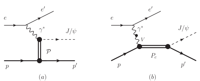
Figure 1: Diagrams for the electroproduction of heavy quarkonium $J/\psi$. (a): The contribution of $t$-channel Pomeron exchange. (b): pentaquark $P_{c}$ production in $s$-channel, where $V$ stands for the all possible vector mesons.

II.1 Pomeron exchange

The Pomeron exchange model Donnachie:1987pu ; Pichowsky:1996jx ; Laget:1994ba accounts for the dominant contribution in the leptoproduction process. The Pomeron mediates the long range interaction between the nucleon and the confined (anti-)quarks within the quarkonium. This is an effective and useful model to parameterize the diffractive process for the production of neutral vector mesons in the high energy region. By including a double Regge pole with intercept equal to one, the soft dipole Pomeron model does not violate unitarity bounds and can describe nearly all available cross-sections data of photo- and electro-production of vector meson from light to heavy and from near threshold to high energies region in a consistent manner Martynov:2002ez .

We start from the photoproduction of vector meson $V$ off proton in the soft dipole Pomeron model with the formula of $t$-dependence cross section Martynov:2002ez

$$\frac{d\sigma}{dt}=4\pi\,|\mathcal{M}^{\mathcal{P}}_{\gamma p\to Vp}|^{2},$$ (1)

where the amplitudes are defined as

$$\mathcal{M}^{\mathcal{P}}_{\gamma p\to Vp} = \mathcal{P}(z,t,M_{V}^{2},Q^{2})+\mathcal{F}(z,t,M_{V}^{2},Q^{2}),$$ (2)

$$\mathcal{P}(z,t,M_{V}^{2},Q^{2}) = ig_{0}(-iz)^{\alpha_{P}(t)-1}+ig_{1}\textrm{ln}(-iz)(-iz)^{\alpha_{P}(t)-1},$$ (3)

$$\mathcal{F}(z,t,M_{V}^{2},Q^{2}) = ig_{f}(-iz)^{\alpha_{f}(t)-1}.$$ (4)

The $\mathcal{P}$ and $\mathcal{F}$ terms are the so called dipole Pomeron and Reggeon. The $Q^{2}=-q^{2}$ and $M_{V}$ are photon virtuality and mass of vector meson, respectively. The variable $z\sim\cos\theta$ with $\theta$ being the scattering angle of final states in c.m. system of $\gamma^{*}p$. The nonlinear Pomeron trajectory is $\alpha_{\mathbb{P}}(t)=1+\gamma(\sqrt{4m_{\pi}^{2}}-\sqrt{4m_{\pi}^{2}-t})$ with $m_{\pi}$ the pion mass and the Reggeon trajectory is $\alpha_{f}(t)=\alpha_{f}(0)+\alpha^{\prime}_{f}(0)t$ with $\alpha_{f}(0)=0.8$ and $\alpha^{\prime}_{f}(0)=0.85\;\text{GeV}^{-2}$. The parameters $\gamma=0.05\;\text{GeV}^{-1}$, $g_{0}=-0.03$, $g_{1}=0.01$ and $g_{f}=0.08$ can be obtained by fitting the vector meson photoproduction. More details can be found in Ref. Martynov:2002ez . The advantage of this model is that it includes exclusive photoproduction of all vector mesons for both real and virtual photons, as shown in above amplitudes. This is convenient for our calculation of electroproduction here. The results for the $J/\psi$ photoproduction are shown in Fig. 2.

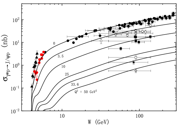
Figure 2: The photonproduction cross section in terms of the invariant mass of $J/\psi$ proton system. The near-threshold data with error bar is the experimental measurements from GlueX Ali:2019lzf (solid triangle), SLAC Camerini:1975cy (red circle), while the other data is from H1 Aid:1996dn ; Adloff:1999zs ; Adloff:2000vm and ZEUS Breitweg:1998nh ; Chekanov:2002xi . The line is the fit from dipole Pomeron.

The electroproduction amplitude for the Pomeron exchange is evaluated as

$$\mathcal{M}_{ep\to eVp} = M_{R_{1}}^{\mu}\frac{-g_{\mu\nu}}{q^{2}}\mathcal{M}_{R_{2}}^{\nu},$$ (5)

where $R_{1}$ is the sub-reaction $e\to e\gamma$ and $M_{R_{1}}^{\mu}=ie\bar{u}(k^{\prime})\gamma^{\mu}u(k)$, while $R_{2}$ is the sub-reaction $\gamma p\to Vp$. If neglecting polarization correlations between the two sub-reactions, we have the amplitude square

$$|\mathcal{M}_{ep\to eVp}|^{2} = \frac{1}{3(q^{2})^{2}}\sum_{\lambda_{1},\lambda_{2}}|M_{R_{1}}^{\mu}\epsilon_{\mu}^{*\lambda_{1}}|^{2}|\mathcal{M}_{R_{2}}^{\nu}\epsilon_{\nu}^{\lambda_{2}}|^{2},$$ (6)

where $\epsilon$ is the polarization vector of intermediate photon with spin of $z$-direction $\lambda_{1,2}$. The amplitude for the sub-reaction $R_{2}$ can be determined from the differential cross section $d\sigma/dt$ by dipole Pomeron model mentioned in Eq. (1) with the relation $|\mathcal{M}^{\mathcal{P}}_{\gamma p\to Vp}|^{2}=\sum_{\lambda_{2}}|\mathcal{M}_{R_{2}}^{\nu}\epsilon_{\nu}^{\lambda_{2}}|^{2}$. Alternative approach to investigate the electroproduction of vector meson is using a microscopic description of the Pomeron exchange Donnachie:1984xq ; Kim:2020wrd .

II.2 Pentaquark

Here we only consider the $P_{c}$ with quantum numbers $\frac{3}{2}^{-}$ in line with the GlueX Ali:2019lzf , where the branching fractions were determined by using the JPAC model Blin:2016dlf . Similar conclusion would be driven for alternative assignment of $J^{P}$. The effective Lagrangian for the coupling of $P_{c}$ to $J/\psi p$ is written as Cao:2010ji ; Wu:2019adv

$${\cal L}^{3/2^{-}}_{VBR} = g\overline{B}\mbox{\boldmath$\tau\!\!$ \unboldmath}\cdot\mbox{\boldmath$V^{\mu}\!\!$ \unboldmath}R_{\mu}+h.c.,$$ (7)

where $R$ and $B$ denote $P_{c}$ resonance and the nucleon, respectively. The coupling constant $g$ can be determined from the corresponding decay widths. Here we use the total decay widths of $P_{c}$ as the measured values by LHCb and the upper limits of branching fractions $\mathcal{B}(P_{c}\to J/\psi p)$ determined by GlueX Ali:2019lzf . The propagator of $P_{c}$ can be written as

$$G^{3/2}_{R}(p_{R}) = \frac{-i(\not\!p_{R}+M_{R})G_{\mu\nu}(p_{R})}{p_{R}^{2}-M^{2}_{R}+iM_{R}\Gamma_{R}},$$ (8)

where $p_{R}$ is the momentum of the propagator, and $M_{R}$ the mass, $\Gamma_{R}$ the decay width of $P_{c}$. The term $G_{\mu\nu}(p_{R})$ is defined as

$$G_{\mu\nu}(p_{R}) = -g_{\mu\nu}+\frac{1}{3}\gamma_{\mu}\gamma_{\nu}+\frac{1}{3M_{R}}(\gamma_{\mu}p_{R\nu}-\gamma_{\nu}p_{R\mu})+\frac{2}{3p_{R}^{2}}p_{R\mu}p_{R\nu}.$$ (9)

We assume that the pentaquark resonances couple to photon via the vector meson pole by using VMD model. Therefore the $\gamma p\to P_{c}$ vertex can be considered as $\gamma p\to Vp\to P_{c}$ as shown in Fig 1(b). The coupling of vector meson to photon is

$$\mathcal{L}_{V\gamma}=\sum_{V}\frac{eM_{V}^{2}}{f_{V}}V_{\mu}A^{\mu},$$ (10)

where $M_{V}$ is the mass of vector meson, and $V^{\mu}$ and $A^{\mu}$ are the vector meson and photon field, respectively. Then the coupling constant of vector meson to photon $e/f_{V}$ can be extracted from the partial decay width $\Gamma_{V\to e^{+}e^{-}}$ from the formula

$$\frac{e}{f_{V}}=\left[\frac{3\Gamma_{V\to e^{+}e^{-}}}{2\alpha_{em}|{\bf p}_{e}|}\right]^{\frac{1}{2}},$$ (11)

where the mass of electron and positron have been neglected, and ${\bf p}_{e}$ is the three-vector momentum of electron in the vector meson rest frame.

For the off-shell vector meson in VMD, we choose the form factor

$$\mathcal{F}(q^{2})=\frac{\Lambda^{4}}{\Lambda^{4}+(q^{2}-M_{V}^{2})^{2}},$$ (12)

where $\Lambda$ is the cut-off parameter. The choice of the vector meson and the cut-off parameter would not change the distribution of the final state, which is the main concern here. Thus we choose the vector meson to be $J/\psi$ and the cutoff $\Lambda=0.5$ GeV.

III Results and discussions

	$M$ [MeV]	$\Gamma$ [MeV]	$J^{P}$
$P_{c}$(4312)	$4311.9\pm 0.7^{+6.8}_{-0.6}$	$9.8\pm 2.7^{+3.7}_{-4.5}$	$\frac{3}{2}^{-}$
$P_{c}$(4440)	$4440.3\pm 1.3^{+4.1}_{-4.7}$	$20.6\pm 4.9^{+8.7}_{-10.1}$	$\frac{3}{2}^{-}$
$P_{c}$(4457)	$4457.3\pm 0.6^{+4.1}_{-1.7}$	$6.4\pm 2.0^{+5.7}_{-1.9}$	$\frac{3}{2}^{-}$

Table 1: The measured masses and widths by LHCb Aaij:2019vzc , while the quantum numbers are taken to be in line with the GlueX Ali:2019lzf since the branching fractions were used here.

We explore the electroproduction of the pentaquarks observed by LHCb Collaboration as listed in Tab. 1, together with the contributions from Pomeron exchange, at JLab12 and EicC energy configurations. JLab12 is the fixed-target experiment with $12$ GeV electron and rest proton, while EicC is the colliding one with $3.5$ GeV electron and $20$ GeV proton. The pentaquark and Pomeron contributions were added incoherently. The interference terms may have large contribution on the total cross section of pentaquark, but distribute smoothly in phase space. Also it is too premature to consider the interference at present, because we do not know the relative phase between different contributions. Most importantly, these terms can be neglected for searching pentaquark since we will focus on the pentaquark dominant phase space area, from which we will get the main conclusion in this paper. In our calculation, we choose the laboratory frame with the electron moving in opposite $z$ direction. The cross sections were evaluated by using the VEGAS program Lepage:1977sw which numerically integrates the kinematic events generated by RAMBO Kleiss:1985gy with the dynamics described by the formula above. Besides that, we get the final state distributions at the same time.

The total production cross sections for both JLab12 and EicC are shown in Tab. 2. We can see that the cross sections of non-resonant background are a few orders of magnitude larger than that of pentaquarks. For the cross section of pentaquarks, the model-dependent branching fractons determined by GlueX and the cut-off parameter in the form factor appear as overall factor, which means the cross sectons rather than the final state distributions are greatly model-dependent. Thus the distributions are our main concern here.

Table 2: The electroproduction cross section (in unit of pb) of pentaquarks and non-resonant backgound at JLab12 and EicC.

	Background	Pentaquarks
JLab12	1.4	0.0016
EicC	111	0.013

The three-momentum and polar angle distributions of the final proton from either Pomeron exchange process or pentaquark production are shown separately in Fig. 3 at JLab12 case and in Fig. 4 at EicC, respectively. The left panels are for the final proton from Pomeron contribution, while the right ones are for the proton from the pentaquark decay. For a better comparison, we use the same range in axes of the two panels for each figure. Due to the totally different energy configuration, the final proton moves in the electron and proton forward angle at JLab12 and EicC, respectively. As we can see, the polar angle distributions of final proton are very different for Pomeron exchange and pentaquark production. This is because the $t$-dependent cross section in Eq. (1) is suppressed at large $t$ for Pomeron exchange, while the shape from pentaquarks is all flat across the full $t$ range. This fact has been already pointed out by several papers Wang:2015jsa ; Cao:2019kst ; Wu:2019adv that the final particles from different contributions have different behaviour at large angles.

In both energy configurations of JLab12 and EicC, the distribution of proton decaying from pentaquarks are quite similar in shape but different in range. The three pentaquarks are characteristic by the obvious resonant bands. Among them, the $P_{c}$(4457) and $P_{c}$(4440) overlap with each other because of their closeness of masses, so a quite good energy resolution is needed to distinguish them. This is a challenge for future detector design.

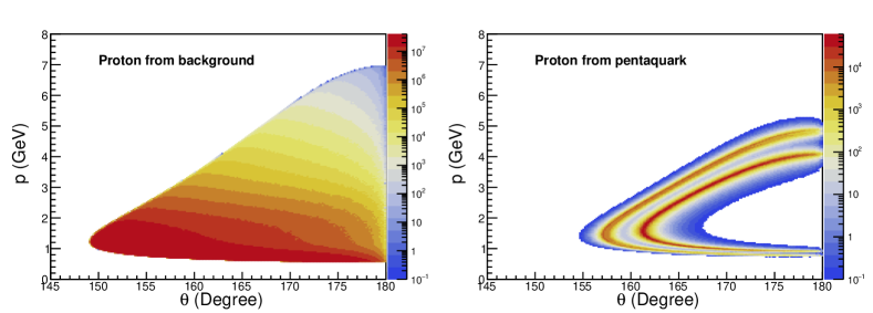
Figure 3: The distribution of momentum versus scattering angles of final proton in the laboratory frame at the JLab energy configuration, with 12 GeV electron beam projectile on rest proton. We set the electron beam moving in opposite $z$ direction. The left panel is the final proton from Pomeron exchange, while the right one is from pentaquark. The colors represent the differential cross section.

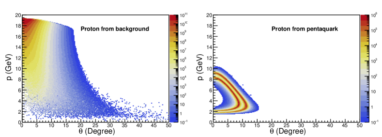
Figure 4: Same as Fig. 3 but at EicC energy configuration, which is 20 GeV proton colliding with 3.5 GeV electron. For a better comparison, we choose the same range in axis of the two panels.

Most importantly, for each energy configuration, the proton from non-resonance background and pentaquark present significant differences in phase space shown in Fig. 3 and Fig. 4. As a result, we can take advantage of this feature to enhance the $P_{c}$ peaks relative to that of the Pomeron exchange. It comes along with the main conclusion of this paper in Fig. 5, which shows the differential cross section of the electroproduction process at the energy configuration of JLab12 and EicC. The dashed and solid curves in Fig. 5 show the results with and without the cut on the three-momentum and angle of final proton, respectively. As we can see, a simple cut $p>3\;\text{GeV}$ can remove much more Pomeron contribution than pentaquark for JLab12. While for EicC, the cut $p<10\;\text{GeV}$ and $\theta>5^{\circ}$ also works very well to depress the background. Quantitatively, in the case of $P_{c}(4312)$ at JLab12, a signal over background ratio increases from 0.3 to 19 with the kinematic cut. Therefore the kinematic cut can make the $P_{c}$ peaks obviously more prominent and present the huge potential in experimental analysis although the total number of events would decrease after the cuts are used. More complex cuts would make the situation much better.

At last we want to emphasize the great potential of both EicC and JLab12 to search for the pentaquark. EicC has a higher signal over background ratio, while JLab12 has much higher luminosity. The center of mass energy of EicC is about 16.7 GeV, much larger than 4.8 GeV of JLab12. As shown in Tab. 2, the larger center of mass energy would make the total cross section 8 and 80 times larger for pentaquark signal and non-resonant background, respectively. However EicC has 15 times larger phase space in the invariant mass $W$ for the background than JLab. Therefore the pentaquark signal could be presented more prominently in the differential cross section at EicC in Fig. 5. On the other hand, the differential cross section is less reduced at EicC than that at JLab12 after the kinematic cut is employed, which shows that colliding mode could be better to study pentaquark than fixed-target mode.

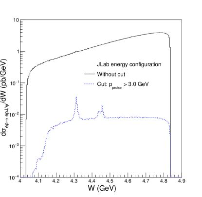
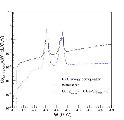
Figure 5: The differential cross section of the electroproduction process in terms of the invariant mass of $J/\psi$ proton system at JLab (left) and EicC (right), respectively. The solid and dashed lines are for the one without and with the cut, respectively. The peaks correspond to the three pentaquarks.

IV Summary

The GlueX Collaboration at JLab has searched for the pentaquark photoproduction and got negative result at present precision Ali:2019lzf . One possibility is that the pentaquark signal is small in total cross section compared to the non-resonant contribution. The production rates have been already investigated in many efforts Cao:2019kst ; Wu:2019adv and the signal of pentaquark in hidden charm photoproduction would be really small in cross sections.

In this paper, we calculated the $ep\to e^{\prime}p^{\prime}J/\psi$ process with both non-resonant $t$-channel contribution and hidden charm pentaquark in $s$-channel. After the non-resonant contribution is normalized using the soft dipole Pomeron model by photoproduction data, the distribution of final particles from both sources were investigated. In view of the very different shape of final proton in phase space owing to the different underlying mechanism, we proposed that the three-momentum and angle cuts on proton could largely suppress the non-resonant contribution and the signal/background ratio would be significantly increased. For both energy configuration of JLab12 and EicC, we found promising strategies even with simple cuts, which is very helpful for future experimental analysis of the electroproduction at these machines. In addition, it is also promising to search for pentaquark at higher energy collider, e.g. US EIC. Similar cut like the one used for EicC would also be helpful. Our criterion is also enlightening for the electroproduction of $P_{b}$, bottom analog of $P_{c}$ states Cao:2019gqo .

Here we focus on the method to depress the background rather than the total production cross section of pentaquarks, because the total cross section of pentaqurks is greatly model-dependent due to the unknown coupling constant and cut-off parameter appearing as overall factors. Last but not least, we shall point out that our framework could be used in the full simulation, the selection criterion of final particles and optimization of detector design in the future.

References

- (1) R. Aaij et al. [LHCb Collaboration], Phys. Rev. Lett. 115, 072001 (2015) doi:10.1103/PhysRevLett.115.072001 [arXiv:1507.03414 [hep-ex]].
- (2) R. Aaij et al. [LHCb Collaboration], Phys. Rev. Lett. 122, no. 22, 222001 (2019) doi:10.1103/PhysRevLett.122.222001 [arXiv:1904.03947 [hep-ex]].
- (3) M. L. Du, V. Baru, F. K. Guo, C. Hanhart, U. G. Meißner, J. A. Oller and Q. Wang, Phys. Rev. Lett. 124, no. 7, 072001 (2020) doi:10.1103/PhysRevLett.124.072001 [arXiv:1910.11846 [hep-ph]].
- (4) C. W. Xiao, J. Nieves and E. Oset, Phys. Lett. B 799, 135051 (2019) doi:10.1016/j.physletb.2019.135051 [arXiv:1906.09010 [hep-ph]].
- (5) C. J. Xiao, Y. Huang, Y. B. Dong, L. S. Geng and D. Y. Chen, Phys. Rev. D 100, no. 1, 014022 (2019) doi:10.1103/PhysRevD.100.014022 [arXiv:1904.00872 [hep-ph]].
- (6) L. Meng, B. Wang, G. J. Wang and S. L. Zhu, Phys. Rev. D 100, no. 1, 014031 (2019) doi:10.1103/PhysRevD.100.014031 [arXiv:1905.04113 [hep-ph]].
- (7) T. J. Burns and E. S. Swanson, Phys. Rev. D 100, no. 11, 114033 (2019) doi:10.1103/PhysRevD.100.114033 [arXiv:1908.03528 [hep-ph]].
- (8) Y. J. Xu, C. Y. Cui, Y. L. Liu and M. Q. Huang, arXiv:1907.05097 [hep-ph].
- (9) G. J. Wang, L. Y. Xiao, R. Chen, X. H. Liu, X. Liu and S. L. Zhu, arXiv:1911.09613 [hep-ph].
- (10) H. Xu, Q. Li, C. H. Chang and G. L. Wang, Phys. Rev. D 101, no. 5, 054037 (2020) doi:10.1103/PhysRevD.101.054037 [arXiv:2001.02980 [hep-ph]].
- (11) J. B. Cheng and Y. R. Liu, Phys. Rev. D 100, no. 5, 054002 (2019) doi:10.1103/PhysRevD.100.054002 [arXiv:1905.08605 [hep-ph]].
- (12) R. Zhu, X. Liu, H. Huang and C. F. Qiao, Phys. Lett. B 797, 134869 (2019) doi:10.1016/j.physletb.2019.134869 [arXiv:1904.10285 [hep-ph]].
- (13) J. R. Zhang, Eur. Phys. J. C 79, no. 12, 1001 (2019) doi:10.1140/epjc/s10052-019-7529-2 [arXiv:1904.10711 [hep-ph]].
- (14) R. Chen, Z. F. Sun, X. Liu and S. L. Zhu, Phys. Rev. D 100, no. 1, 011502 (2019) doi:10.1103/PhysRevD.100.011502 [arXiv:1903.11013 [hep-ph]].
- (15) M. Z. Liu, Y. W. Pan, F. Z. Peng, M. Sánchez Sánchez, L. S. Geng, A. Hosaka and M. Pavon Valderrama, Phys. Rev. Lett. 122, no. 24, 242001 (2019) doi:10.1103/PhysRevLett.122.242001 [arXiv:1903.11560 [hep-ph]].
- (16) H. X. Chen, W. Chen and S. L. Zhu, Phys. Rev. D 100, no. 5, 051501 (2019) doi:10.1103/PhysRevD.100.051501 [arXiv:1903.11001 [hep-ph]].
- (17) J. He, Eur. Phys. J. C 79, no. 5, 393 (2019) doi:10.1140/epjc/s10052-019-6906-1 [arXiv:1903.11872 [hep-ph]].
- (18) M. I. Eides, V. Y. Petrov and M. V. Polyakov, arXiv:1904.11616 [hep-ph].
- (19) A. Ali and A. Y. Parkhomenko, Phys. Lett. B 793, 365 (2019) doi:10.1016/j.physletb.2019.05.002 [arXiv:1904.00446 [hep-ph]].
- (20) A. Ali, I. Ahmed, M. J. Aslam, A. Y. Parkhomenko and A. Rehman, JHEP 1910, 256 (2019) doi:10.1007/JHEP10(2019)256 [arXiv:1907.06507 [hep-ph]].
- (21) Z. G. Wang, Int. J. Mod. Phys. A 35, no. 01, 2050003 (2020) doi:10.1142/S0217751X20500037 [arXiv:1905.02892 [hep-ph]].
- (22) C. Fernández-Ramírez et al. [JPAC Collaboration], Phys. Rev. Lett. 123, no. 9, 092001 (2019) doi:10.1103/PhysRevLett.123.092001 [arXiv:1904.10021 [hep-ph]].
- (23) Y. Yamaguchi, H. García-Tecocoatzi, A. Giachino, A. Hosaka, E. Santopinto, S. Takeuchi and M. Takizawa, arXiv:1907.04684 [hep-ph].
- (24) M. Pavon Valderrama, Phys. Rev. D 100, no. 9, 094028 (2019) doi:10.1103/PhysRevD.100.094028 [arXiv:1907.05294 [hep-ph]].
- (25) J. J. Wu, R. Molina, E. Oset and B. S. Zou, Phys. Rev. Lett. 105, 232001 (2010) doi:10.1103/PhysRevLett.105.232001 [arXiv:1007.0573 [nucl-th]].
- (26) J. J. Wu, R. Molina, E. Oset and B. S. Zou, Phys. Rev. C 84, 015202 (2011) doi:10.1103/PhysRevC.84.015202 [arXiv:1011.2399 [nucl-th]].
- (27) J. J. Wu and T.-S. H. Lee, Phys. Rev. C 86, 065203 (2012) doi:10.1103/PhysRevC.86.065203 [arXiv:1210.6009 [nucl-th]].
- (28) C. W. Shen, D. Rönchen, U. G. Meißner and B. S. Zou, Chin. Phys. C 42, no. 2, 023106 (2018) doi:10.1088/1674-1137/42/2/023106 [arXiv:1710.03885 [hep-ph]].
- (29) C. W. Xiao and E. Oset, Eur. Phys. J. A 49, 139 (2013) doi:10.1140/epja/i2013-13139-y [arXiv:1305.0786 [hep-ph]].
- (30) M. Karliner and J. L. Rosner, Phys. Rev. Lett. 115, no. 12, 122001 (2015) doi:10.1103/PhysRevLett.115.122001 [arXiv:1506.06386 [hep-ph]].
- (31) H. X. Chen, W. Chen, X. Liu and S. L. Zhu, Phys. Rept. 639, 1 (2016) doi:10.1016/j.physrep.2016.05.004 [arXiv:1601.02092 [hep-ph]].
- (32) F. K. Guo, C. Hanhart, U. G. Meißner, Q. Wang, Q. Zhao and B. S. Zou, Rev. Mod. Phys. 90, no. 1, 015004 (2018) doi:10.1103/RevModPhys.90.015004 [arXiv:1705.00141 [hep-ph]].
- (33) R. F. Lebed, R. E. Mitchell and E. S. Swanson, Prog. Part. Nucl. Phys. 93, 143 (2017) doi:10.1016/j.ppnp.2016.11.003 [arXiv:1610.04528 [hep-ph]].
- (34) A. Esposito, A. Pilloni and A. D. Polosa, Phys. Rept. 668, 1 (2017) doi:10.1016/j.physrep.2016.11.002 [arXiv:1611.07920 [hep-ph]].
- (35) S. L. Olsen, T. Skwarnicki and D. Zieminska, Rev. Mod. Phys. 90, no. 1, 015003 (2018) doi:10.1103/RevModPhys.90.015003 [arXiv:1708.04012 [hep-ph]].
- (36) Y. R. Liu, H. X. Chen, W. Chen, X. Liu and S. L. Zhu, Prog. Part. Nucl. Phys. 107, 237 (2019) doi:10.1016/j.ppnp.2019.04.003 [arXiv:1903.11976 [hep-ph]].
- (37) N. Brambilla, S. Eidelman, C. Hanhart, A. Nefediev, C. P. Shen, C. E. Thomas, A. Vairo and C. Z. Yuan, arXiv:1907.07583 [hep-ex].
- (38) A. Ali, J. S. Lange and S. Stone, Prog. Part. Nucl. Phys. 97, 123 (2017) doi:10.1016/j.ppnp.2017.08.003 [arXiv:1706.00610 [hep-ph]].
- (39) F. K. Guo, X. H. Liu and S. Sakai, doi:10.1016/j.ppnp.2020.103757 arXiv:1912.07030 [hep-ph].
- (40) F. K. Guo, U. G. Meißner, W. Wang and Z. Yang, Phys. Rev. D 92, no. 7, 071502 (2015) doi:10.1103/PhysRevD.92.071502 [arXiv:1507.04950 [hep-ph]].
- (41) X. H. Liu, Q. Wang and Q. Zhao, Phys. Lett. B 757, 231 (2016) doi:10.1016/j.physletb.2016.03.089 [arXiv:1507.05359 [hep-ph]].
- (42) F. K. Guo, H. J. Jing, U. G. Meißner and S. Sakai, Phys. Rev. D 99, no. 9, 091501 (2019) doi:10.1103/PhysRevD.99.091501 [arXiv:1903.11503 [hep-ph]].
- (43) Y. H. Lin and B. S. Zou, Phys. Rev. D 100, no. 5, 056005 (2019) doi:10.1103/PhysRevD.100.056005 [arXiv:1908.05309 [hep-ph]].
- (44) S. Sakai, H. J. Jing and F. K. Guo, Phys. Rev. D 100, no. 7, 074007 (2019) doi:10.1103/PhysRevD.100.074007 [arXiv:1907.03414 [hep-ph]].
- (45) D. Winney et al. [JPAC Collaboration], Phys. Rev. D 100, no. 3, 034019 (2019) doi:10.1103/PhysRevD.100.034019 [arXiv:1907.09393 [hep-ph]].
- (46) H. X. Chen, arXiv:2001.09563 [hep-ph].
- (47) J. J. Wu, T.-S. H. Lee and B. S. Zou, Phys. Rev. C 100, no. 3, 035206 (2019) doi:10.1103/PhysRevC.100.035206 [arXiv:1906.05375 [nucl-th]].
- (48) Q. Wu and D. Y. Chen, Phys. Rev. D 100, no. 11, 114002 (2019) doi:10.1103/PhysRevD.100.114002 [arXiv:1906.02480 [hep-ph]].
- (49) X. Y. Wang, X. R. Chen and J. He, Phys. Rev. D 99, no. 11, 114007 (2019) doi:10.1103/PhysRevD.99.114007 [arXiv:1904.11706 [hep-ph]].
- (50) Z. H. Guo and J. A. Oller, Phys. Lett. B 793, 144 (2019) doi:10.1016/j.physletb.2019.04.053 [arXiv:1904.00851 [hep-ph]].
- (51) Q. Wang, X. H. Liu and Q. Zhao, Phys. Rev. D 92, 034022 (2015) doi:10.1103/PhysRevD.92.034022 [arXiv:1508.00339 [hep-ph]].
- (52) Y. Huang, J. J. Xie, J. He, X. Chen and H. F. Zhang, Chin. Phys. C 40, no. 12, 124104 (2016) doi:10.1088/1674-1137/40/12/124104 [arXiv:1604.05969 [nucl-th]].
- (53) A. N. Hiller Blin, C. Fernández-Ramírez, A. Jackura, V. Mathieu, V. I. Mokeev, A. Pilloni and A. P. Szczepaniak, Phys. Rev. D 94, no. 3, 034002 (2016) doi:10.1103/PhysRevD.94.034002 [arXiv:1606.08912 [hep-ph]].
- (54) M. Karliner and J. L. Rosner, Phys. Lett. B 752, 329 (2016) doi:10.1016/j.physletb.2015.11.068 [arXiv:1508.01496 [hep-ph]].
- (55) V. Kubarovsky and M. B. Voloshin, Phys. Rev. D 92, no. 3, 031502 (2015) doi:10.1103/PhysRevD.92.031502 [arXiv:1508.00888 [hep-ph]].
- (56) Q. F. Lü, X. Y. Wang, J. J. Xie, X. R. Chen and Y. B. Dong, Phys. Rev. D 93, no. 3, 034009 (2016) doi:10.1103/PhysRevD.93.034009 [arXiv:1510.06271 [hep-ph]].
- (57) X. H. Liu and M. Oka, Nucl. Phys. A 954, 352 (2016) doi:10.1016/j.nuclphysa.2016.04.040 [arXiv:1602.07069 [hep-ph]].
- (58) S. H. Kim, H. C. Kim and A. Hosaka, Phys. Lett. B 763, 358 (2016) doi:10.1016/j.physletb.2016.10.061 [arXiv:1605.02919 [hep-ph]].
- (59) X. Y. Wang, J. He, X. R. Chen, Q. Wang and X. Zhu, Phys. Lett. B 797, 134862 (2019) doi:10.1016/j.physletb.2019.134862 [arXiv:1906.04044 [hep-ph]].
- (60) Z. E. Meziani et al., arXiv:1609.00676 [hep-ex].
- (61) A. Ali et al. [GlueX Collaboration], Phys. Rev. Lett. 123, no. 7, 072001 (2019) doi:10.1103/PhysRevLett.123.072001 [arXiv:1905.10811 [nucl-ex]].
- (62) X. Cao and J. p. Dai, Phys. Rev. D 100, no. 5, 054033 (2019) doi:10.1103/PhysRevD.100.054033 [arXiv:1904.06015 [hep-ph]].
- (63) Xu Cao, Lei Chang, Ningbo Chang, et al., Nuclear Techniques, 2020, 43(2): 020001. doi:10.11889/j.0253-3219.2020.hjs.43.020001.
- (64) X. Cao, F. K. Guo, Y. T. Liang, J. J. Wu, J. J. Xie, Y. P. Xie, Z. Yang and B. S. Zou, arXiv:1912.12054 [hep-ph].
- (65) E. Martynov, E. Predazzi and A. Prokudin, Phys. Rev. D 67, 074023 (2003) doi:10.1103/PhysRevD.67.074023 [hep-ph/0207272].
- (66) B. S. Zou and F. Hussain, Phys. Rev. C 67, 015204 (2003) doi:10.1103/PhysRevC.67.015204 [hep-ph/0210164].
- (67) X. Cao, B. S. Zou and H. S. Xu, Nucl. Phys. A 861, 23 (2011) doi:10.1016/j.nuclphysa.2011.05.094 [arXiv:1009.1060 [nucl-th]].
- (68) X. Cao, B. S. Zou and H. S. Xu, Int. J. Mod. Phys. A 26, 505 (2011) doi:10.1142/S0217751X11051901 [arXiv:1009.1063 [nucl-th]].
- (69) X. Cao, B. S. Zou and H. S. Xu, Phys. Rev. C 81, 065201 (2010) doi:10.1103/PhysRevC.81.065201 [arXiv:1004.0140 [nucl-th]].
- (70) A. Donnachie and P. V. Landshoff, Phys. Lett. B 185, 403 (1987). doi:10.1016/0370-2693(87)91024-0
- (71) M. A. Pichowsky and T. S. H. Lee, Phys. Lett. B 379, 1 (1996) doi:10.1016/0370-2693(96)00440-6 [nucl-th/9601032].
- (72) J. M. Laget and R. Mendez-Galain, Nucl. Phys. A 581, 397 (1995). doi:10.1016/0375-9474(94)00428-P
- (73) U. Camerini et al., Phys. Rev. Lett. 35, 483 (1975). doi:10.1103/PhysRevLett.35.483
- (74) S. Aid et al. [H1 Collaboration], Nucl. Phys. B 472, 3 (1996) doi:10.1016/0550-3213(96)00274-X [hep-ex/9603005].
- (75) C. Adloff et al. [H1 Collaboration], Eur. Phys. J. C 10, 373 (1999) doi:10.1007/s100520050762 [hep-ex/9903008].
- (76) C. Adloff et al. [H1 Collaboration], Phys. Lett. B 483, 23 (2000) doi:10.1016/S0370-2693(00)00530-X [hep-ex/0003020].
- (77) J. Breitweg et al. [ZEUS Collaboration], Eur. Phys. J. C 6, 603 (1999) doi:10.1007/s100529901051 [hep-ex/9808020].
- (78) S. Chekanov et al. [ZEUS Collaboration], Eur. Phys. J. C 24, 345 (2002) doi:10.1007/s10052-002-0953-7 [hep-ex/0201043].
- (79) A. Donnachie and P. V. Landshoff, Nucl. Phys. B 244, 322 (1984). doi:10.1016/0550-3213(84)90315-8
- (80) S. H. Kim and S. i. Nam, arXiv:2003.03589 [hep-ph].
- (81) G. P. Lepage, J. Comput. Phys. 27, 192 (1978). doi:10.1016/0021-9991(78)90004-9
- (82) R. Kleiss, W. J. Stirling and S. D. Ellis, Comput. Phys. Commun. 40, 359 (1986). doi:10.1016/0010-4655(86)90119-0