Multi-Frequency Observations of the Candidate Neutrino Emitting Blazar BZB J0955+3551

Abstract

The recent spatial and temporal coincidence of the blazar TXS 0506+056 with the IceCube detected neutrino event IC-170922A has opened up a realm of multi-messenger astronomy with blazar jets as a plausible site of cosmic-ray acceleration. After TXS 0506+056, a second blazar, BZB J0955+3551, has recently been found to be spatially coincident with the IceCube detected neutrino event IC-200107A and undergoing its brightest X-ray flare measured so far. Here, we present the results of our multi-frequency campaign to study this peculiar event that includes observations with the NuSTAR, Swift, NICER, and 10.4 m Gran Telescopio Canarias (GTC). The optical spectroscopic observation from GTC secured its redshift as $z=0.55703^{+0.00033}_{-0.00021}$ and the central black hole mass as 10^8.90±0.16 $M_{\odot}$. Both NuSTAR and NICER data reveal a rapid flux variability albeit at low-significance ($\lesssim 3.5\sigma$). We explore the origin of the target photon field needed for the photo-pion production using analytical calculations and considering the observed optical-to-X-ray flux level. We conclude that seed photons may originate from outside the jet, similar to that reported for TXS 0506+056, although a scenario invoking a co-moving target photon field (e.g., electron-synchrotron) can not be ruled out. The electromagnetic output from the neutrino-producing photo-hadronic processes are likely to make only a sub-dominant contribution to the observed spectral energy distribution suggesting that the X-ray flaring event may not be directly connected with IC-200107A.

1 Introduction

High-energy neutrinos are unique messengers originating from the extreme physical processes in the Universe. Being solely produced in hadronic interactions of high-energy cosmic-ray nuclei with ambient matter or photon fields, they provide the smoking gun signature for hadronic acceleration sites.

Blazars, i.e., radio-loud quasars with powerful relativistic jets aligned to our line of sight, have been suggested as potential cosmic-ray and neutrino sources (see, e.g., Mannheim et al., 1992; Petropoulou et al., 2015; Murase, 2017; Lucarelli et al., 2019; Garrappa et al., 2019; Franckowiak et al., 2020). The most compelling high-energy neutrino source candidate identified so far is the blazar TXS 0506+056 (IceCube Collaboration et al., 2018a, b). The 290 TeV neutrino IC-170922A was found in spatial coincidence with TXS 0506+056 and arrived during a major outburst observable in all wavelengths (IceCube Collaboration et al., 2018a). Interestingly an archival search for lower-energy $\mathcal{O}$(10 TeV) neutrinos revealed a neutrino flare in 2014/15, which lasted 160 days, but was not accompanied by activity in the electromagnetic regime (IceCube Collaboration et al., 2018b). From a theoretical perspective, Reimer et al. (2019) proposed that there should not be a strongly correlated gamma-ray and neutrino activity, and that neutrino production activity (through associated cascading) might actually show up more clearly in X-rays. However, the conclusion about the $\gamma$-ray/PeV neutrino correlation is reported to be model-dependent (see, e.g., Rodrigues et al., 2019; Zhang et al., 2020).

BL Lacertae objects (or BL Lacs) are a sub-population of blazars that exhibits an optical spectrum lacking any emission lines with equivalent width $>5$Å (e.g., Stickel et al., 1991). Their optical spectra are power-law dominated indicating either especially strong non-thermal continuum (due to Doppler boosting) or unusually weak thermal disk/broad line emission (plausibly attributed to low accretion activity; Giommi et al., 2012). BL Lacs that have the synchrotron peak located at very high frequencies ($\nu^{\rm peak}_{\rm syn}\geq 10^{17}$ Hz) are termed as extreme blazars (e.g., Costamante et al., 2001; Foffano et al., 2019; Paliya et al., 2019a). The observation of such a high synchrotron peak frequency indicates them to host some of the most efficient particle accelerator jets. Interestingly, extreme blazars are also proposed as promising candidates of high-energy neutrinos (cf. Petropoulou et al., 2015; Padovani et al., 2016).

So far, any clustering of neutrinos in either space or time have not been confirmed in the all-sky searches of IceCube data (Aartsen et al., 2015, 2017a, 2020). Therefore, a promising methodology could be the search for transient and variable electromagnetic sources temporally and spatially coincident with IceCube neutrino events using multi-frequency observations.

In this regard, the identification of a $\gamma$-ray detected extreme blazar, BZB J0955+3551 (also known as 4FGL J0955.1+3551), found in spatial coincidence with the IceCube detected neutrino event IC-200107A (IceCube Collaboration, 2020; Giommi et al., 2020; Krauss et al., 2020) has provided an interesting case for blazar jets as a plausible source of cosmic neutrinos. In fact, a prompt Swift-XRT target of opportunity (ToO) observation of BZB J0955+3551 on 2020 January 8 found it to be undergoing its brightest X-ray flare measured so far. Another $\gamma$-ray detected blazar, 4FGL J0957.8+3423, was found to lie within the 90% positional uncertainty of IC-200107A, however, no significant flux enhancement was noticed from this object in X- or $\gamma$-rays (Krauss et al., 2020; Garrappa et al., 2020).

Motivated by the identification of a candidate neutrino emitting blazar undergoing an X-ray outburst close in time to the neutrino arrival, we started a multi-wavelength campaign. This includes a Director’s Discretionary Time (DDT) observation with the Nuclear Spectroscopic Telescope Array (NuSTAR) and multiple Swift target of opportunity (ToO) observations. An optical spectroscopic followup with 10.4 m Gran Telescopio Canarias (GTC) was carried out to determine the spectroscopic redshift of BZB J0955+3551. In addition to that, the source was also observed with the Neutron star Interior Composition Explorer (NICER) simultaneous to the NuSTAR pointing as a part of DDT ToO invoked by the mission principal investigator. Here, we present the results of the conducted multi-frequency campaign and attempt a theoretical interpretation to understand the underlying physical processes. In Section 2, we describe the steps adopted to analyze various data sets. Results are presented in Section 3 and discussed in Section 4. We summarize our findings in Section 5. Throughout, we adopt a Cosmology of $H_{0}=67.8$ km s^-1 Mpc^-1, $\Omega_{m}=0.308$, and $\Omega_{\Lambda}=0.692$ (Planck Collaboration et al., 2016).

2 Data Reduction and Analysis

2.1 Optical Spectroscopy with GTC

The $i^{\prime}$ filter image of BZB J0955+3551 taken with the Panoramic Survey Telescope and Rapid Response System (Pan-STARRS) is shown in Figure 1. A faint companion object ($i^{\prime}$ magnitude = 20.85$\pm$0.36) located $\sim$3^′′ South-East of the blazar ($i^{\prime}$ magnitude = 19.17$\pm$0.06) can be seen. Since both objects lacked spectroscopic redshift information, we carried out a long-slit spectroscopy of the system with Optical System for Imaging and low-Intermediate-Resolution Integrated Spectroscopy (OSIRIS; Cepa et al., 2000, 2003) spectrograph mounted at GTC.

The 0.8 arcsec-wide slit was positioned to cover the source and a companion $\sim$3 arcsec south-east to the blazar (see Figure 1). The total integration time was $\sim$2 hrs divided into 6 exposures of 1098 s each. The chosen grism was R1000R, which covers the spectral range of 5100 - 10000 Å with a resolution ($\lambda/\Delta\lambda$) of 1122. This grism was selected due to its large spectral range and good spectral resolution, which provides a large pool to find emission or absorption lines and calculate the redshift of the source.

The raw data was reduced using the standard procedure with the IRAF tasks, through the PyRAF software. The main steps are: bias and flat correction, cosmic-ray removal, wavelength calibration, sky subtraction, spectra extraction and flux calibration. The cosmic rays were removed in each individual science spectrum with the IRAF task lacos_spec (van Dokkum, 2001). The wavelength calibration was done with a combination of arcs from three different lamps (Hg-Ar, Ne and Xe) to cover all the wavelength range of the spectra. The sky was subtracted with the IRAF task background, selecting background samples to the right of the blazar and to the left on the companion, and fitted with a Chebyshev polynomial of order 3. After this step, the science spectra were combined, which removed any cosmic-ray residual. The spectrum of the blazar and the companion were extracted independently from the combined science spectra. The extraction was done with the IRAF task apall, optimising the apertures to extract the most flux from the sources. For the flux calibration, the spectrophotometric standard star G191-B2B was observed on the same night of the observation. This calibration included atmospheric extinction correction at the observatory (King, 1985). Each spectrum was flux calibrated to convert from counts to absolute flux units, and corrected from Galactic extinction using the IRAF task deredden with the values $\mathrm{R}=3.1$, $\mathrm{E(B-V)}=0.0109$ (Schlafly & Finkbeiner, 2011).

2.2 NuSTAR, NICER, and Swift

NuSTAR observed BZB J0955+3551 on 2020 January 11 for a net exposure of 25.6 ksec under our DDT request (observation id: 90501658002, PI: Paliya). We first cleaned and calibrated the event file using the tool nupipeline. We define the source and background regions as circles of 30^′′ and 70^′′, respectively. The former was centered at the target blazar and the latter from a nearby region on the same chip and avoiding source contamination. The pipeline nuproducts was used to extract light curves, spectra, and ancillary response files. In the energy range of 3$-$79 keV, a binning of 1.5 ksec was adopted to generate the light curve and the source spectrum was binned to have at least 20 counts per bin.

NICER observed BZB J0955+3551  for a net exposure of $\sim$11 ksec, simultaneous to the NuSTAR pointing on 2020 January 11 as a DDT target of opportunity (ToO observation id: 2200990102). We analyzed the NICER data with the latest software HEASOFT 6.26.1 and calibration files (v. 20190516). In particular, the pipeline nicerl2 was adopted with default settings to selects all 56 detectors, apply standard filters and calibration to clean the events and finally merge them to generate one event file. We then used the tool xselect to extract the source spectrum and 3 minutes binned light curve. The background was estimated using the tool nicer_bkg_estimator (K. Gendreau et al. in preparation). The quasar spectrum was binned to 20 counts per bin.

Close in time to the arrival of IC-200107A neutrino, ToO observations of BZB J0955+3551 from the Swift satellite were carried out on 2020 January 8 (Giommi et al., 2020; Krauss et al., 2020), 10 and 11. We first cleaned and calibrated the X-ray Telescope (XRT) data taken in the photon counting mode with the tool xrtpipeline and by adopting the latest CALDB (v. 20200106). Exposure maps and ancillary response files were generated with the tasks ximage and xrtmkarf, respectively. To extract the source spectrum, we considered a circular region of 47^′′, which encloses about 90% of the XRT point spread function, centered at the target. The background was estimated from an annular region centered at the target with inner and outer radii 70^′′ and 150^′′, respectively. We binned the blazar spectrum to 20 counts per bin. The X-ray spectral analysis was carried out in XSPEC (Arnaud, 1996) and the Galactic neutral hydrogen column density ($N_{\rm H}=1.14\times 10^{20}$ cm^-2) was adopted from Kalberla et al. (2005).

Individual snapshots taken from the Swift UltraViolet Optical Telescope (UVOT) were first combined using the pipeline uvotimsum and then photometry was performed with the task uvotsource. For the latter, we considered a source region of 2^′′, avoiding the nearby object located $\sim$3^′′ South-East of BZB J0955+3551. The background is estimated from a 30 ^′′ circular region free from the source contamination. The derived magnitudes were corrected for Galactic extinction (Schlafly & Finkbeiner, 2011) and converted to flux units following zero points adopted from Breeveld et al. (2011).

2.3 Others

BZB J0955+3551 remained below the detection threshold of the Fermi-Large Area Telescope at the time of the neutrino arrival and prior on month-to-years timescale (Garrappa et al., 2020). Therefore, we used the spectral parameters provided in the recently released fourth catalog of the Fermi-LAT detected objects (4FGL; Abdollahi et al., 2020) to get an idea about the average $\gamma$-ray behavior of the source. In addition to that, we used archival measurements from the Space Science Data Center. These datasets can provide a meaningful information about the typical activity state of the source.

2.4 Probability of chance coincidence

The third catalog of high-synchrotron peaked blazars (3HSP; Chang et al., 2019) contains 384 extreme blazars, yielding a density of $9.3\times 10^{-3}$ per sq. deg. of sky. Since the total number of extreme blazars are predicted to be $\sim$400 (Chang et al., 2019), the sample of extreme blazars present in the 3HSP catalog can be considered almost complete. Given that IC200107A had a 90% localization of 7.6 deg, we thus expect to find $7.1\times 10^{-2}$ extreme blazars coincident with the neutrino.

We can additionally determine the X-ray flare rate or duty cycle (DC) for extreme blazars, as for any other class of astrophysical objects, using the X-ray variability information collected from an all-sky surveying instrument. For this we used publicly available 2$-$12 keV light curves generated using the data from the All Sky Monitor (ASM) on board the Rossi X-ray Timing Explorer (RXTE) mission. We cross-matched the RXTE ASM catalog of 587 sources with 3HSP, and found ASM light curves for 17 extreme blazars. To avoid spurious detection due to poor sensitivity of the instrument, for each object, we considered only data points which qualified the following two filters: (i) the count rate ($R_{\rm ASM}$) should be positive, and (ii) $R_{\rm ASM}/\Delta R_{\rm ASM}>$2, where $\Delta R_{\rm ASM}$ is the 1$\sigma$ uncertainty in $R_{\rm ASM}$. Furthermore, the observation on a particular day was considered as a flare if the count rate estimated for that day of observation ($R_{\rm ASM,i}$) fulfilled the following condition:

$$R_{\rm ASM,i}-\Delta R_{\rm ASM,i}\geq 2\times\langle R_{\rm ASM}\rangle$$ (1)

where $\langle R_{\rm ASM}\rangle$ is the median count rate for the mission light curve. If the observation on a particular day qualified the above mentioned filter (Equation 1), we flagged it as a ‘flare’, otherwise ‘non-flare’. The DC is then computed as the ratio of the number of flaring epochs divided by total observing epochs. This exercise led to the mean DC for the sample as 5.2% with a range of 1.7-8.9%. Assuming the mean DC of these 17 extreme blazars is representative of the broader extreme blazar population, the probability of finding a coincident extreme blazar by chance that is simultaneously flaring in X-rays is just $3.7\times 10^{-3}$. This estimate is, however, specific to IC200107A. The possibility that other high-energy neutrinos may have had flaring extreme blazar counterparts is difficult to quantify without a systematic follow-up program.

2.5 Neutrino flux estimate

A single high-energy neutrino detection from the extreme blazar population would suggest a cumulative expectation of 0.05 $<N_{\textup{pop}}<$ 4.74 at 90% confidence, with each of the 384 extreme blazars contributing some fraction of this total (Strotjohann et al., 2019). If each had an equal likelihood to generate a neutrino alert, then we would expect $1.3\times 10^{-4}\lesssim N_{\textup{src}}\lesssim 0.012$ per extreme blazar.

Given that the association with BZB J0955+3551  is not dependent on the event topology of IC200107A, we simply require sufficient neutrino flux for a single high-energy neutrino alert under any of the public IceCube realtime alert selections. IC200107A was identified by a new neural network classifier (IceCube Collaboration, 2020), which identifies high-energy starting track events with high efficiency (Kronmueller & Glauch, 2019). However, with an overall rate of high-energy starting tracks that is just $\sim$2 per year (IceCube Collaboration, 2020), the effective area for this selection is still substantially smaller than that for through-going muon alerts (Blaufuss et al., 2019).

We can derive the necessary neutrino fluence normalization taking the sum of neutrino effective areas at the declination of BZB J0955+3551  over the duration of the Icecube Realtime System. For this 4 year period, which overlaps a transition in IceCube event selections, we integrate each effective area over the period that they were active (Aartsen et al., 2017b; Blaufuss et al., 2019). No neutrino energy estimate was provided for IC200107A (IceCube Collaboration, 2020), so we here assume an approximate neutrino energy of $\sim$100 TeV, the energy at which most starting tracks are expected for an $E^{-2}$ spectrum. The effective area at this energy was 0.7 m² under the old alert selection(Aartsen et al., 2017b), and 9.48 m² under the new alert selection (Blaufuss et al., 2019), yielding a weighted average of 2.9 m² at the declination of the source. With this effective area, at 100 TeV, we require a mean neutrino flux of $6\times 10^{-15}<F_{\textup{steady}}<5\times 10^{-13}$ ${\rm\,erg\,\,cm^{-2}\,s^{-1}}$ for extreme blazars such as BZB J0955+3551. If we assume neutrino emission from these sources is dominated by X-ray flares, then for a DC of 5.2% we expect a flux of $1\times 10^{-13}<F_{\textup{flare}}<1\times 10^{-11}$ erg cm^-2 s^-1 for the duration of each flare. Given the large range of the expected neutrino flux, we conservatively assume a value of 10^-13 ${\rm\,erg\,\,cm^{-2}\,s^{-1}}$ for rest of the calculation, considering an Eddington bias of a factor of 100 (Strotjohann et al., 2019).

3 Results

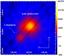
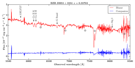
Figure 1: Left: Pan-STARRS $i^{\prime}$ filter image of BZB J0955+3551. Note the presence of a faint companion object at $\sim$3^′′ South-East of the blazar. Parallel black lines represent the slit position for the long-slit spectrograph OSIRIS. The colorbar represents the Pan-STARRS count units. Right: Optical spectra of the source BZB J0955+3551 and the companion taken at GTC with OSIRIS. The red line is the spectrum of the blazar and the blue line is the spectrum of the companion. The identified emission and absorption lines are marked with vertical arrows and labeled correspondingly. The atmospheric absorption features are marked with the symbol $\oplus$.

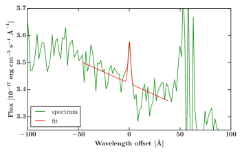
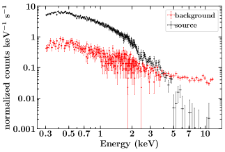
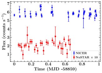
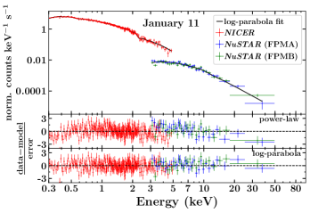
Figure 2: Top left: Fit of the emission line [OII]3727 to derive its luminosity and equivalent width. The spectrum is shown in a green line and the fit in a red line. The continuum is fit with a polynomial of degree 1 and the line with a single Gaussian function. The wavelength of the line has been subtracted from the x-axis. Top right: NICER count spectra of BZB J0955+3551 (black) and the background (red). As can be seen, at $\gtrsim 5$ keV, the background dominates the observed counts. Bottom left: 1.5 ksec binned NuSTAR (3$-$79 keV) and 3 minutes binned NICER (0.3$-$5 keV) light curves of BZB J0955+3551. The flux of the former is multiplied by 10 for a meaningful comparison. Bottom right: The NICER and NuSTAR counts spectrum jointly fitted with the best-fitted log-parabola model. Lower panels show the residuals of the fit for two models: power-law and log-parabola, as labeled.

The optical spectra of BZB J0955+3551 and the nearby companion are shown in Figure 1. Various absorption lines associated with the host galaxy, e.g., Ca II H&K doublet, are identified in the optical spectrum of the blazar. Additionally, we also detected a weak [O II]3727 emission line. These allowed us to firmly establish the redshift of BZB J0955+3551 as $z=0.55703^{+0.00033}_{-0.00021}$. The spectrum of the companion does not reveal any noticeable feature. Deeper spectroscopic observations are necessary to characterize this object and to explore the possibility of its interaction/merger with BZB J0955+3551.

We computed the rest-frame equivalent width of the [OII]3727 emission line by fitting the continuum around the emission line with a polynomial of degree 1 and the emission line with a Gaussian function (see top left panel in Figure 2). The data was normalized by the factor $10^{-17}$. We first fitted the continuum with a sample of 45 points, $\sim$30 and $\sim$40 Å  to either side of the line. With the continuum subtracted from the spectrum, we fitted the emission line using 7 points ($\sim 11$Å), more than the three free parameters in the fit. This leads to the rest-frame equivalent width of 0.15$\pm$0.05 Å and line luminosity as $(6\pm 2)\times 10^{39}$ erg s^-1. Note that the signal-to-noise ratio around [OII]3727 line is $>$70 which ensures that the estimated values are reliable. Moreover, during the analysis, we varied the extraction aperture, which changed the amount of sky residuals in the final spectrum, to determine if the observed emission line could be due to background noise. In all cases, the line was clearly visible. Therefore, we conclude that the line detection is real and free from any artifacts.

In order to ascertain the impact of the background on the NICER observation, we plot the count spectrum of the source and background in Figure 2 (top right panel). As can be seen, the NICER spectrum remains source dominated up to $\sim$5 keV. Therefore, we used 0.3$-$5 keV energy range to extract the NICER light curve and spectrum of BZB J0955+3551.

In the bottom left panel of Figure 2, we show the NICER and the NuSTAR light curves. The light curves are scanned to search for rapid flux variations. This was done by computing the flux doubling/halving time ($\tau$) as follows:

$$F(t_{2})=F(t_{1})2^{(t_{2}-t_{1})/\tau}$$ (2)

where $F(t_{1})$ and $F(t_{2})$ are the fluxes at time $t_{1}$ and $t_{2}$ respectively. The uncertainties in the flux values were taken into account by setting the conditions that the difference in fluxes at the epochs $t_{1}$ and $t_{2}$ is at least 2$\sigma$ significant.

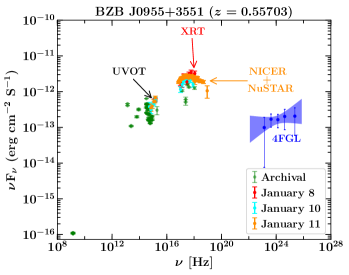
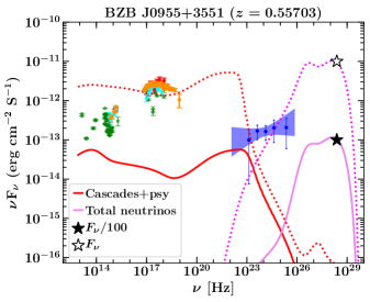
Figure 3: Left: Broadband SED of BZB J0955+3551 generated using the data acquired on January 8 (red) and 11 (yellow) and also considering archival observations (green). In the Fermi-LAT energy range, we show the bow-tie and spectral data points adopted from the 4FGL catalog. Right: Same as left but plotting the results of the hadronic simulation performed using the parameters constrained from the observed optical-to-X-ray spectrum and derived from the analytical calculations in Section 4.2. We divide the expected 100 TeV neutrino flux of $1\times 10^{-11}$ ${\rm\,erg\,\,cm^{-2}\,s^{-1}}$ (black empty star) by a factor of 100 (black filled star) to take into account the Eddington bias (cf. Strotjohann et al., 2019).

Table 1: Summary of the SED analysis.

				X-ray
Epoch	$\Gamma_{\rm X}/\alpha$	$\beta$	Normalization	Flux	$chi^{2}$/dof	Prob.	Instrument
January 8	1.74${}^{+0.11}_{-0.10}$	–	14.11${}^{+1.03}_{-1.03}$	5.37${}^{+0.97}_{-0.77}$	22.93/27	0.6	Swift-XRT
January 10	2.83${}^{+0.44}_{-0.38}$	1.10${}^{0.54}_{0.49}$	1.17${}^{+0.21}_{-0.22}$	1.89${}^{+0.67}_{-0.48}$	14.07/21	$<10^{-4}$	Swift-XRT
January 11	2.13${}^{+0.04}_{-0.04}$	0.17${}^{+0.04}_{-0.03}$	1.74${}^{+0.08}_{-0.07}$	3.80${}^{+0.14}_{-0.17}$	456.94/462	$<10^{-4}$	NICER+NuSTAR
				2.11${}^{+0.21}_{-0.15}$
			Swift-UVOT
Epoch	$V$	$B$	$U$	$UVW1$	$UVM2$	$UVW2$
January 8	–	–	–	–	5.75$\pm$0.56	6.03$\pm$0.54
January 10	3.78$\pm$1.24	3.13$\pm$0.70	4.03$\pm$0.59	4.58$\pm$0.58	5.54$\pm$0.55	6.23$\pm$0.70
January 11	–	3.54$\pm$0.72	3.91$\pm$0.58	5.20$\pm$0.72	5.36$\pm$0.51	6.75$\pm$0.74

We found evidence of rapid flux variations in the NICER data with the shortest flux halving time of 28.3$\pm$7.9 minutes at 3.5$\sigma$ significance level. The NuSTAR light curve also revealed traces of fast variability with the shortest flux doubling time of 19.2$\pm$10.7 minutes, albeit at a low 2.2$\sigma$ confidence level.

In order to search for curvature in the X-ray spectrum, we fitted two models, a power-law and a log-parabola, taking into account the Galactic absorption. The goodness of the fit was determined using f-test. The results of the spectral analysis are provided in Table 1 and residuals of the fit are shown in Figure 2 (bottom right panel). The XRT spectrum taken on January 8 is well explained with a simple absorbed power-law model, whereas, that of January 10 is better fitted with the log-parabola model. The joint NICER and NuSTAR spectrum from January 11 is also well explained with an absorbed log-parabola model, clearly revealing the synchrotron peak. Note that we do not use Swift-XRT data in the January 11 spectral fitting due to two reasons: (i) the fit is dominated by NICER and NuSTAR spectra because of much better photon statistics, and (ii) after removing bad channels (using ignore bad command in XSPEC), Swift-XRT spectrum is limited up to 5 keV, thus giving no advantage over NICER observation.

The broadband spectral energy distribution (SED) of BZB J0955+3551 during the January 8, 10, and 11 epochs are shown in Figure 3. The archival IR-optical spectrum reveals a bump which is likely to be originated from the host galaxy and has been noticed in many extreme blazars (see, e.g., Costamante et al., 2018). The long-time averaged 4FGL SED reveals an extremely hard $\gamma$-ray spectrum suggesting the inverse Compton peak to be located at very high energies ($>$100 GeV). Note that at this redshift the extragalactic background light attenuation is also significant (Domínguez et al., 2011; Paliya et al., 2019a).

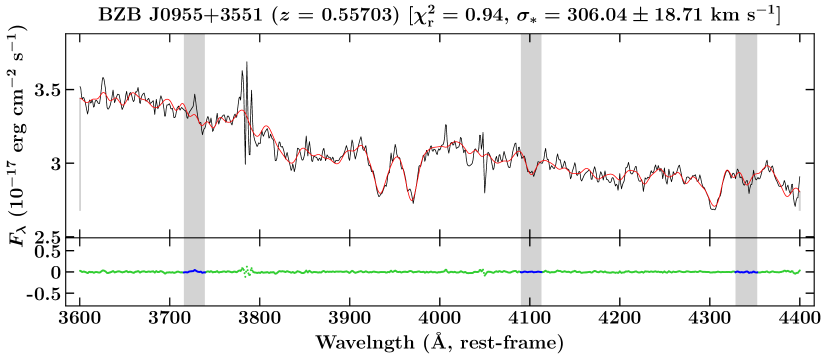
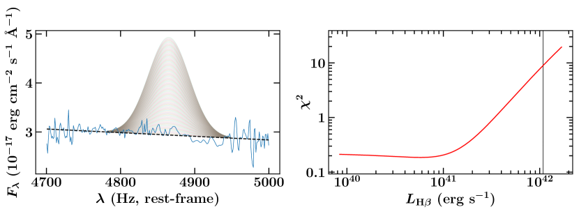
Figure 4: Top: Optical spectrum of BZB J0955+3551 (black line) fitted with the stellar population synthesis tool pPXF (red line). The bottom panel refers to the residual of the fit. The grey shaded area denote the wavelength regions excluded from the fit to mask emission lines. The derived stellar velocity dispersion and the reduced $\chi^{2}$ are quoted. Bottom: The rest-frame OSIRIS spectrum (blue solid line, left panel) when fitted with a power-law (black dashed line) and a single Gaussian function with variable $L_{\rm H\beta}$. The right panel shows the variation of the derived $\chi^{2}$ as a function of $L_{\rm H\beta}$. The vertical black solid line highlights the $L_{\rm H\beta}$ value beyond which $\chi^{2}>\chi^{2}$ (99.7%).

4 Discussion

4.1 Properties of the Central Engine

We have used the well-calibrated empirical relation between the black hole mass ($M_{\rm BH}$) and the central stellar velocity dispersion ($\sigma_{*}$) to determine the former (cf. Gültekin et al., 2009; Kormendy & Ho, 2013). To determine $\sigma_{*}$, we used the penalized PiXel Fitting software (pPXF; Cappellari & Emsellem, 2004). This tool works in pixel space and adopts a maximum penalized likelihood approach to derive the line-of-sight velocity distribution (LOSVD) from kinematic data (Merritt, 1997). To fit the galaxy spectrum, pPXF uses a large set of single stellar population spectral libraries which we adopted from Vazdekis et al. (2010). It first creates a template galaxy spectrum by convolving the stellar population models with the parameterized LOSVD and then fit the model on the observed galaxy spectrum by minimizing $\chi^{2}$. We also added a fourth-order Legendre polynomial to account for the likely featureless contribution from the nuclear emission. From the best-fit spectrum, pPXF computes $\sigma_{*}$ and associated 1$\sigma$ uncertainty. The result of this analysis is shown in Figure 4 and the derived $\sigma_{*}$ is $306.04\pm 18.71$ km s^-1.

We used the following empirical relation to compute $M_{\rm BH}$ (Gültekin et al., 2009):

$$\log{\left(\frac{M_{\rm BH}}{M_{\odot}}\right)}=(8.12\pm 0.08)+(4.24\pm 0.41)\log{\left(\frac{\sigma_{*}}{200~{}\mathrm{km~{}s^{-1}}}\right)},$$ (3)

By supplying the $\sigma_{*}$ derived from the pPXF fit in the above equation, the mass of the central black hole is obtained as $\log M_{\rm BH,\odot}=8.90\pm 0.16$. The quoted uncertainty is statistical only and does not include the intrinsic scatter ($\sim$0.4 dex) associated with this method (Gültekin et al., 2009).

Since no broad emission lines are detected in the optical spectrum of BZB J0955+3551, we have determined 3$\sigma$ upper limit on the broad line region (BLR) luminosity ($L_{\rm BLR}$) by adopting the following procedure. The OSIRIS spectrum was analyzed in the rest-frame wavelength range [4700, 5000] Å where H_β emission line is expected to be present. We brought the spectrum to the rest-frame and fitted with a power-law to reproduce the continuum. We assumed the H$\beta$ emission line as a Gaussian with variable luminosity while keeping its full width at half maximum fixed to 4000 km s^-1, a value typical for blazars (cf. Shaw et al., 2012). Then, a $\chi^{2}$ test was performed by fitting the Gaussian model on the data by varying the line luminosity ($L_{\rm H\beta}$). We computed the upper limit to $L_{\rm H\beta}$ when $\chi^{2}>\chi^{2}$ (99.7%), i.e., at 3$\sigma$ confidence level. The derived upper limit on $L_{\rm H\beta}$ is $1.1\times 10^{42}$ erg s^-1. This is demonstrated in the bottom panel of Figure 4. Furthermore, by adopting the line flux ratios from Francis et al. (1991) and Celotti et al. (1997), we estimated the $L_{\rm BLR}$ upper limit as $\sim$2.7$\times$10⁴³ erg s^-1. The presence of a more luminous BLR can be ruled out as that would emit stronger emission lines which should be observed in the optical spectrum. Furthermore, the inferred $L_{\rm BLR}$ implies an accretion rate (in Eddington units) of $L_{\rm BLR}/L_{\rm Edd}\lesssim 0.0003$. Such a low-accretion rate suggests a radiatively inefficient accretion process and is expected in BL Lac objects.

4.2 General theoretical considerations

The following section considers general energetic requirements for the production of a detectable IceCube neutrino flux in the jet of BZB J0955+3551. These are constrained by the observed UV – X-ray flux just after the detection of the neutrino event, on 2020 January 8 and are similar to that reported for neutrino production in TXS 0506+056 by Reimer et al. (2019). Specifically a flux around $\sim 10^{16}$ – $10^{17}$ Hz of $\nu F_{\nu}^{UV-X}\sim 10^{-12}\,F_{UV,-12}$ erg cm^-2 s^-1 was observed, while the peak of the X-ray spectrum was located around $\sim 10^{18}$ Hz at a flux close to $\nu F_{\nu}\sim 3\times 10^{-12}$ erg cm^-2 s${}^{-1}\equiv 10^{-12}\,F_{X,-12}$ erg cm^-2 s^-1 with $F_{X,-12}\sim 3$. We first derive a general constraint on the jet content of protons that might potentially be responsible for very high-energy (VHE) neutrino production, and then consider two possibilities for the source of target photons for photo-pion production on those protons.

The neutrino emission region propagates along the jet with Lorentz factor $\Gamma=10\,\Gamma_{1}$, leading to Doppler boosting characterized by a Doppler factor $D=10\,D_{1}$. The observed sub-hour-scale X-ray variability suggests a size of the X-ray emission region of $R_{X}\lesssim 3.5\times 10^{14}\,D_{1}$ cm. As our analytical and numerical modeling results below will demonstrate, it is unlikely that the observed X-ray emission has been produced in the same (photo-hadronic and cascade) processes as the neutrino emission. Hence, the neutrino emission region region may be different from that producing X-rays. Assuming a neutrino emission region of the size mentioned above would lead to an unrealistically high compactness, with the required relativistic proton pressure exceeding the magnetic pressure by many orders of magnitude. For example, the assumed production of the observed neutrino flux through photo-pion processes requires characteristic proton powers of $L_{\rm p}\sim 10^{48}-10^{49}$ erg s^-1. Writing $L_{\rm p}=10^{48}L_{48}$ erg s^-1, the energy density in relativistic protons is then $u^{\prime}_{\rm p}\sim 10^{3}L_{48}/(R_{\rm 16}^{2}$) erg cm^-3 assuming a proton escape time scale of $t^{\prime}_{\rm esc}=10^{7}$ sec (see Böttcher et al., 2013, for details). Assuming relativistic protons, the pressure exerted by protons us $p^{\prime}_{\rm p}\sim u^{\prime}_{\rm p}/3\sim 350L_{48}/(R_{16}^{2}$) dyne cm^-2. The magnetic pressure, on the other hand, is $p^{\prime}_{\rm B}\sim 400B_{2}^{2}$ dyne cm^-2. Thus, for an emission region size $\ll$10¹⁶ cm, the proton pressure will exceed the magnetic pressure for any plausible value of the magnetic field. Thus, confinement of the emission region in such a small volume appears implausible. We therefore assume that neutrinos are produced in a larger emission region of size $R\sim 10^{16}\,R_{16}$ cm. In the following, primes denote quantities in the rest-frame of this emission region. The redshift of $z=0.5573$ corresponds to a luminosity distance of $d_{L}\sim 3.2\,{\rm Gpc}\sim 9.7\times 10^{27}$ cm.

4.3 Proton-photon interactions and neutrino production

In AGN jets, neutrinos are most plausibly produced through photo-hadronic interactions of relativistic protons of energy $E^{\prime}_{p}=\gamma_{p}\,m_{p}c^{2}$ with target photons of energy $E^{\prime}_{t}$. This interaction is most efficient when the center-of-momentum frame energy squared, $s=(m_{p}c^{2})^{2}+2\,E^{\prime}_{p}\,E^{\prime}_{t}\,(1-\beta_{p}\cos\theta)$ — where $\beta_{p}=\sqrt{1-1/\gamma_{p}^{2}}$ is the normalized velocity (in units of the speed of light c) and $\gamma_{p}$ the Lorentz factor of the proton — of the interaction is near the $\Delta^{+}$ resonance, $s\sim E_{\Delta^{+}}^{2}=(1232{\rm MeV})^{2}$, where the $p\gamma$ interaction cross section peaks. This translates into a condition $E^{\prime}_{p}\,E^{\prime}_{t}\sim 3.2\times 10^{5}\,{\rm MeV}^{2}$.

The proton energy required to produce neutrinos at observed (i.e., Doppler-boosted) energies of hundreds of TeV, $E_{\nu}\equiv 100\,E_{14}$ TeV ($E_{14}$ is the neutrino energy in units of $10^{14}$ eV) is $E^{\prime}_{p}\simeq 200\,E_{14}/(D_{1}\,\xi_{0.05})$ TeV (i.e., $\gamma^{\prime}_{p}=E^{\prime}_{p}/m_{p}c^{2}\simeq 2\times 10^{5}E_{14}/(D_{1}\,\xi_{0.05})$) where $\xi\equiv 0.05\,\xi_{0.05}$ is the average neutrino energy per initial proton energy in photo-hadronic interactions (Mücke et al., 1999). The Larmor radius of protons with such energy is $r_{L}\sim 6.7\times 10^{10}\,(\gamma_{p}^{\prime}/[2\times 10^{5}])\,B_{2}^{-1}$ cm, where $B=100\,B_{2}$ G is the magnetic field. This indicates that they are expected to be well confined within the emission region and can plausibly be accelerated by standard mechanisms.

For photo-pion (and neutrino) production by protons of this energy at the $\Delta^{+}$ resonance, target photons of $E^{\prime}_{t}\geq 1.6D_{1}\xi_{0.05}/E_{14}$ keV are required. In section 4.5, we will discuss two extreme options for the source of such target photons: (a) the co-moving electron synchrotron radiation field, and (b) an external radiation field that is isotropic in the AGN rest frame. First, however, we derive constraints on the number of relativistic protons that may be present in the jet.

4.4 Constraints on Jet Power

Protons of energy $E^{\prime}_{p}=200\,E_{14}/(D_{1}\,\xi_{0.05})$ TeV radiate proton synchrotron radiation at a characteristic frequency of

$$\nu_{\rm psy}^{\rm obs}=4.2\times 10^{6}\,B_{G}\,\gamma_{p}^{2}\,D\,(m_{e}/m_{p})\;{\rm Hz}$$

$$\approx 9.2\times 10^{16}\,{B_{2}\,E_{14}^{2}\over D_{1}\,\xi_{0.05}^{2}}\;{\rm Hz},$$ (4)

i.e., in soft X-rays. Given a number of protons of energy $\gamma_{p}$, i.e., $N_{p}(\gamma_{p})\sim\gamma_{p}\,dN_{p}(\gamma_{p})/d\gamma_{p}$, one may calculate the produced co-moving luminosity in proton synchrotron radiation as

$$L^{\prime}_{\rm psy}\approx{c\,\sigma_{T}\,B^{2}\over 6\pi}\,\left({m_{e}\over m_{p}}\right)^{2}\,\gamma_{p}^{3}\,{dN_{p}(\gamma_{p})\over d\gamma_{p}}$$

$$\approx 2.5\times 10^{-2}\,{dN_{p}(\gamma_{p})\over d\gamma_{p}}\,B_{2}^{2}\,{E_{14}^{3}\over D_{1}^{3}\,\xi_{0.05}^{3}}\;{\rm erg\,s}^{-1}.$$ (5)

The resulting observable soft X-ray flux, $\nu F_{\nu}^{\rm psy}\sim D_{1}^{4}\,L^{\prime}_{\rm psy}/(4\,\pi\,d_{L}^{2})$ may not over-shoot the actually observed UV – soft X-ray flux, thus constraining the differential number of protons to

$${dN_{p}(\gamma_{p})\over d\gamma_{p}}\lesssim 4.7\times 10^{42}\,{F_{X,-12}\,\xi_{0.05}^{3}\over B_{2}^{2}\,D_{1}\,E_{14}^{3}}.$$ (6)

We consider a proton spectrum of the form $N_{p}(\gamma_{p})=N_{0}\,\gamma_{p}^{-\alpha_{p}}$ with $\alpha_{p}=2$, extending from $\gamma_{\rm p,min}=1$ to $\gamma_{\rm p,max}\sim 2\times 10^{5}\,E_{14}/(D_{1}\,\xi_{0.05})$ so that the resulting proton synchrotron spectrum actually peaks (in $\nu F_{\nu}$ representation) at the characteristic proton synchrotron frequency $\nu_{\rm psy}$ evaluated in Eq. (4) above. The proton-spectrum normalization is then constrained to

$$N_{0}\lesssim 1.9\times 10^{53}\,{F_{X,-12}\,\xi_{0.05}\over B_{2}^{2}\,D_{1}^{3}\,E_{14}}$$ (7)

limiting the kinetic jet power in relativistic protons to

$$L_{p}\sim{3\,\Gamma^{2}\,c\,(m_{p}c^{2})\,N_{0}\over 4\,R}\,\ln\gamma_{\rm p,max}$$

$$\lesssim 6.4\times 10^{46}\,{F_{X,-12}\,\xi_{0.05}\,\Gamma_{1}^{2}\over B_{2}^{2}\,D_{1}^{3}\,E_{14}\,R_{16}}\,(12.2+\eta)\;{\rm erg\,s}^{-1},$$ (8)

where $\eta\equiv\ln(E_{14}/[D_{1}\,\xi_{0.05})$. For $\eta=0$ and all baseline parameters, Eq. (8) evaluates to $2.3\times 10^{48}$ erg s^-1 for one-sided jet. In the following, we ignore the (presumed small) correction arising from potential values of $\eta\neq 0$.

Using the proton spectrum with normalization given by Eq. (7), we may estimate the co-moving neutrino luminosity through the proton energy loss rate due to photopion production, given by Kelner & Aharonian (2008) (see also Berezinskii & Grigor’eva, 1988; Stanev et al., 2000)

$${\dot{\gamma}}_{\rm p,p\gamma}\approx-c\,\langle\sigma_{p\gamma}f\rangle\,n^{\prime}_{\rm ph}(\epsilon^{\prime}_{t})\,\epsilon^{\prime}_{t}\,\gamma_{p}$$ (9)

where $\epsilon^{\prime}_{t}=E^{\prime}_{t}/(m_{e}c^{2})$ and $\langle\sigma_{p\gamma}f\rangle\approx 10^{-28}$ cm² is the elasticity-weighted p$\gamma$ interaction cross section. The factor $n^{\prime}_{\rm ph}(\epsilon^{\prime}_{t})\,\epsilon^{\prime}_{t}$ provides a proxy for the co-moving energy density of the target photon field, $u^{\prime}_{\rm t}\approx m_{e}c^{2}\,n^{\prime}_{\rm ph}(\epsilon^{\prime}_{t})\,(\epsilon^{\prime}_{t})^{2}$. Considering that the energy lost by protons in p$\gamma$ interactions is shared approximately equally between photons and neutrinos, the VHE neutrino luminosity is given by

$$L^{\prime}_{\nu}\approx{1\over 2}\,N_{0}\,m_{p}c^{2}\,\int\limits_{\gamma_{1}}^{\gamma_{\rm p,max}}\gamma_{p}^{-2}\,\left|{\dot{\gamma}}_{\rm p,p\gamma}\right|\,d\gamma_{p}$$

$$\approx{1\over 2}\,c\,N_{0}\,m_{p}c^{2}\,\langle\sigma_{p\gamma}f\rangle\,{u^{\prime}_{t}\over\epsilon^{\prime}_{t}\,m_{e}c^{2}}\,\ln\left({\gamma_{\rm p,max}\over\gamma_{1}}\right)$$ (10)

Considering that the target photon is unlikely to be mono-energetic, we set the lower limit in the integral in Eq. (10) to $\gamma_{1}=6.4\times 10^{4}/(D_{1}\,\xi_{0.05})$, corresponding to protons producing neutrinos with an observed energy of $\sim 30$ TeV. With this choice, the limit on the neutrino luminosity (corresponding to the limit on $N_{0}$ from Equation 7) evaluates to

$$L^{\prime}_{\nu}\lesssim 1.7\times 10^{41}\,{u^{\prime}_{t}\over{\rm erg\,cm}^{-3}}\ln(3.1\,E_{14})\,{F_{X,-12}\,\over B_{2}^{2}\,D_{1}^{4}}\;{\rm erg\,s}^{-1},$$ (11)

which yields a limit on the VHE neutrino flux measured on Earth as

$$F_{\nu}\lesssim 1.4\times 10^{-12}\,{u^{\prime}_{t}\over{\rm erg\,cm}^{-3}}\,\ln(3.1\,E_{14})\,{F_{X,-12}\over B_{2}^{2}}\;{\rm erg\,cm}^{-2}\,{\rm s}^{-1}.$$ (12)

The single neutrino detection of IC-200107A corresponds to an approximate neutrino energy flux of $F_{\nu}^{\rm obs}\sim 10^{-11}$ erg cm^-2 s^-1 (Section 2.5). Accounting for a possible Eddington bias due to the large number of potentially similar blazars from which no neutrinos have been detected (Strotjohann et al., 2019), the actual neutrino flux from this individual source may, however, be up to a factor of $\sim 100$ lower than the estimate provided above. We, therefore, base our estimates below on a neutrino flux of $F_{\nu}\sim 10^{-13}\,F_{\nu,-13}$ erg cm^-2 s^-1. Thus, Eq. (12) translates into a limit on the co-moving target photon field energy density of

$$u^{\prime}_{t}\gtrsim 6.8\times 10^{-2}\,{B_{2}^{2}\,F_{\nu,-13}\over F_{X,-12}\,\ln(3.1\,E_{14})}\;{\rm erg\,cm}^{-3}.$$ (13)

In the following, we will discuss implications for the nature of such a target photon field.

4.5 Implications on the target photon fields

We will distinguish two possible scenarios, which can be thought of as extreme, limiting cases: (a) a target photon field that is co-moving with the emission region (such as the electron-synchrotron emission), or (b) a stationary target photon field in the AGN rest frame.

4.5.1 a) Co-moving target photon field

If the target photon field is co-moving (e.g., the electron-synchrotron photon field, which is routinely used in lepto-hadronic blazar models as targets for photo-pion production), the target photon energy $E^{\prime}_{t}$ corresponds to an observed photon energy of $E_{\rm t,obs}\geq 16\,D_{1}^{2}\xi_{0.05}/E_{14}$ keV (i.e., hard X-rays). The directly observed X-ray flux corresponding to the co-moving radiation energy density from Eq. (13) is, in this case, Doppler boosted by a factor of $D^{4}$ with respect to the observer, yielding a lower limit on the X-ray flux from this radiation field of

$$F_{t}^{\rm obs,a}\sim{D^{4}\,R^{2}\,c\,u^{\prime}_{t}\over d_{L}^{2}}$$

$$\gtrsim 2.2\times 10^{-11}\,{F_{\nu,-13}\,R_{16}^{2}\,B_{2}^{2}\,D_{1}^{4}\over F_{X,-12}\,\ln(3.1\,E_{14})}\;{\rm erg\,cm}^{-2}\,{\rm s}^{-1}.$$ (14)

Thus, a slightly smaller emission region size than $10^{16}$ cm, a magnetic field of $B<10^{2}$ G, and/or a slightly smaller Doppler factor, $D<10$ might plausibly allow this estimate not to over-predict the observed X-ray flux of $F_{X}\sim 3\times 10^{-12}$ erg cm^-2 s^-1. This is contrary to the case of TXS 0506+056, where the co-moving electron synchrotron radiation field being the dominant target photon field for photo-pion production to produce a significant flux of VHE neutrinos could be safely ruled out (see, e.g., Keivani et al., 2018; Reimer et al., 2019; Rodrigues et al., 2019; Zhang et al., 2020).

4.5.2 b) Stationary photon field in the AGN rest frame

In the case of a photon field that is stationary (and quasi-isotropic) in the AGN rest frame, the external (stationary) target photon field is Doppler boosted into the blob frame, so that $E_{\rm t,obs}\geq 0.16\xi_{0.05}/E_{14}$ keV (i.e., UV-to-soft X-rays). In this case, the target photon density is enhanced in the co-moving frame, compared to the AGN-rest-frame energy density $u_{t}^{\rm AGN}\sim u^{\prime}_{t}/\Gamma^{2}$. Assuming that the target photon field originates in a larger region of size $R_{t}=10^{17}\,R_{t,17}$ cm surrounding the jet, the resulting, directly observable UV – soft X-ray flux amounts to

$$F_{t}^{\rm obs,b}\sim{u^{\prime}_{t}\,R_{t}^{2}\,c\over\Gamma^{2}\,d_{L}^{2}}$$

$$\gtrsim 2.2\times 10^{-15}\,{F_{\nu,-13}\,R_{t,17}^{2}\,B_{2}^{2}\over\Gamma_{1}^{2}\,F_{X,-12}\,\ln(3.1\,E_{14})}\;{\rm erg\,cm}^{-2}\,{\rm s}^{-1}.$$ (15)

For most plausible parameter choices this remains of the order of the observed X-ray flux.

We therefore conclude that a scenario involving a dominant external radiation field as the target for photo-hadronic neutrino production in the jet of BZB J0955+3551 can more easily satisfy all observational constraints. However, a co-moving target photon field (e.g., electron-synchrotron) can not be ruled out or even strongly disfavoured.

Using the 3$\sigma$ upper limit on $L_{\rm BLR}$ derived in Section 4.1, we can determine whether the external photon field needed for neutrino production (Equation 13) could originate from the BLR of BZB J0955+3551. Assuming the emission region being located within a spherical BLR of radius $R_{\rm BLR}$, the comoving frame BLR energy density can be written as follows:

$$u^{\prime}_{\rm BLR}\sim\frac{\Gamma^{2}L_{\rm BLR}}{4\pi R^{2}_{\rm BLR}c}$$ (16)

Adopting $R_{\rm BLR}=R_{t}\sim 10^{17}$ cm and $\Gamma=10$, we get $u^{\prime}_{\rm BLR}\lesssim 0.72$ erg cm^-3. This implies that the BLR could act as a reservoir of seed photons for photo-hadronic neutrino production. However, since a definite value of $L_{\rm BLR}$ could not be ascertained, a strong conclusion cannot be made. Indeed, if we consider the disk luminosity-BLR radius relationship (see e.g., Tavecchio & Ghisellini, 2008), a low level of accretion luminosity of BZB J0955+3551 indicates a small $R_{\rm BLR}$ and, on average, the emission region would be located farther away, as also reported in various blazar population studies (see, e.g., Paliya et al., 2017, 2019b). In the absence of a strong photon field, relativistic electrons can reach up to very high energies leading to the observation of a high synchrotron peaked SED (cf. Ghisellini et al., 2013). Therefore, though plausible, a BLR origin of the external photon field cannot be ascertained with high confidence.

In the following, we will further investigate the possibility of photo-hadronic neutrino production in BZB J0955+3551 with an external target photon field, and check whether the observed optical – UV – X-ray spectrum is consistent with constraints from electromagnetic cascades initiated by the neutrino-producing pion and muon decay processes.

4.6 Numerical Simulations

Following the analytical considerations in the previous sub-sections, we now attempt to reproduce the observed neutrino flux with a detailed numerical model while not overshooting the observed emission. We employ the steady-state, single-zone lepto-hadronic model described in Böttcher et al. (2013), using parameters in agreement with the limits derived from the analytical estimates in the previous sub-section. In the numerical simulation, as described in Böttcher et al. (2013), the code determines the radiating proton spectrum by evaluating an equilibrium between injection of a power-law proton spectrum, escape, and radiative cooling. The escape time scale has been set as a multiple $\eta_{\rm esc}=30$ times the light crossing time scale, i.e., $t^{\prime}_{\rm esc}=\eta_{\rm esc}*R/c$ (in the co-moving frame of the emission region). This is the same for electrons and protons. Numerically, therefore, a proton escape time scale of $t^{\prime}_{\rm esc}=10^{7}$ sec was used in the simulation. The external photon field required for photo-hadronic neutrino production is represented by an equivalent electron-synchrotron radiation field with the same characteristics as the presumed external radiation field in the co-moving frame of the neutrino emission region, because the code of Böttcher et al. (2013) does currently not include external radiation fields for photo-pion production. It has been shown that the anisotropy of the target photon field has a negligible effect on the neutrino production and electromagnetic radiation output. Thus, our equivalent electron-synchrotron radiation set-up is an appropriate proxy for the required external target photon field.

The results of the simulation reproducing the Eddington-bias-corrected neutrino flux of $F_{\nu}\sim 10^{-13}$ erg cm^-2 s^-1 are shown in Figure 3 with red and violet solid lines. The corresponding parameters are listed in Table 2. The choice of the SED parameters was based on the typical values found in previous lepto-hadronic modeling of blazars (Böttcher et al., 2013; Keivani et al., 2018; Reimer et al., 2019; Rodrigues et al., 2019). The very intense target photon field provides a very high $\gamma$$\gamma$ opacity for $\gamma$-rays in the Fermi-LAT energy range and higher, analogous to what was found for TXS 0506+056 (Reimer et al., 2019). This suggests that one would not expect a significant correlation between neutrino and $\gamma$-ray activity. Furthermore, the cascade synchrotron flux is well below the observed optical – UV – X-ray flux, suggesting that all electromagnetic flux components are likely to be produced by different processes and possibly even in a different emission region than the neutrino flux.

The dashed model curves in Figure 3 show an attempt to reproduce the neutrino flux of $10^{-11}$ ${\rm\,erg\,\,cm^{-2}\,s^{-1}}$, i.e., neglecting the Eddington bias. For this purpose, the target photon density was increased by a factor of 36 with respect to the previous simulation, leaving all other parameters unchanged. It is obvious that, in this case, the electromagnetic output from proton synchrotron and cascades overshoots the optical – UV fluxes, and its spectral shape is very different from the observed optical – X-ray spectrum of BZB J0955+3551. This can, therefore, be ruled out.

Overall, our results suggest a scenario in which a relativistic proton population responsible for the observed neutrino emission from BZB J0955+3551 may only make a sub-dominant contribution to the observed X-ray flare. The detection of rapid X-ray flux variability also hints that the neutrino producing region may not be same as the one emitting X-rays. Therefore, we argue that the detection of an X-ray flare from BZB J0955+3551 found close-in-time to IC-200107A is likely a coincidence and the two events may not be physically connected.

A comprehensive analysis of the this neutrino event has also been carried out by Petropoulou et al. (2020) who studied the same event using various lepto-hadronic models with different emission region conditions. Though co-spatial neutrino and electromagnetic radiation producing regions were considered, the neutrino emission was not found to be related with the observed X-ray flare. These results are aligned with our findings derived from analytical calculation and a crude numerical simulation as discussed above. Moreover, among various theoretical models, they also explored a case of hidden external photon field (a putative weak BLR) providing seed photons for photo-hadronic production of neutrinos. In this single-zone lepto-hadronic model with external photon field, they reported that the predicted neutrino flux would be even lower during the X-ray flare to avoid overshooting the observed $\gamma$-ray spectrum (see Petropoulou et al., 2020, for details). These findings are in agreement with that reported in this work.

Table 2: Parameters used/derived from the numerical simulation. The shape of the proton spectrum is adopted as a power law.

Parameter	Value
Co-moving photon field energy density (erg cm-3)	55
Co-moving photon field peak frequency (Hz)	$3.5\times 10^{17}$
Magnetic field (Gauss)	100
Bulk Lorentz factor	10
Emission-region radius (cm)	$1\times 10^{16}$
Viewing angle (degrees)	5.7
Low-energy cut-off of proton spectrum (GeV)	1
Proton high-energy cut-off (GeV)	106
Proton Injection spectral index	1.1
Kinetic luminosity in protons (erg s-1)	$1\times 10^{49}$
Magnetic jet power (erg s-1)	$3.75\times 10^{47}$

Note. — Swift-XRT spectral fitting (January 8 and 10) is done in the energy range of 0.3$-$10 keV, whereas, it is 0.3$-$79 keV for the joint NICER and NuSTAR analysis (January 11). $\Gamma_{\rm X}$ is the power-law X-ray photon index and $\alpha$ and $\beta$ are the log-parabolic photon index at the pivot energy (fixed at 3 keV) and curvature around the peak, respectively. The X-ray normalization has the unit of 10^-4 ${\rm\,ph\,\,cm^{-2}\,s^{-1}}$ keV^-1. The quoted flux values are in 2$-$10 keV energy range and in the second row of January 11 data, we also provide the flux in 10$-$79 keV. The power-law and log-parabola models were compared by adopting f-test and the derived probability of null-hypothesis (that the power-law model is a better representation of the data) is given in the column ‘Prob.’. The flux values reported for the Swift-UVOT filters are in 10^-13 ${\rm\,erg\,\,cm^{-2}\,s^{-1}}$ and are corrected for Galactic reddening.

5 Summary

We have followed the X-ray flaring activity of BZB J0955+3551 (Giommi et al., 2020; Krauss et al., 2020) with NuSTAR, Swift, and GTC and also used the simultaneous observation from NICER. Using the high-quality OSIRIS spectrum, we determined the spectroscopic redshift of the blazar as $z=0.55703^{+0.00033}_{-0.00021}$. On the other hand, we could not ascertain the nature of the companion object identified $\sim$3^′′ South-East of BZB J0955+3551 in the $i^{\prime}$ filter Pan-STARRS image. From the stellar velocity dispersion measured using pPXF, the central black hole mass of BZB J0955+3551 was derived as 10^8.90±0.16 $M_{\odot}$. Moreover, the optical spectrum of the source reveals a faint [O II]3727 emission line with rest-frame equivalent width of 0.15$\pm$0.05 Å. We estimated a very low-level of accretion activity which is consistent with that expected from BL Lac objects. There are tentative evidences ($\lesssim 3.5\sigma$) for the hour-scale flux variability in the X-ray band, as estimated from the NuSTAR and NICER light curves. Finally, we showed that a scenario involving an external photon field as targets for photo-pion production of neutrinos is more easily able to satisfy all observational constraints but a scenario invoking a co-moving target photon field (e.g., electron-synchrotron) can not be ruled out or even strongly disfavored. Any electromagnetic signatures of the photo-pion processes responsible for the neutrino emission, are likely to only make a sub-dominant contribution to the observed electromagnetic radiation from IR to $\gamma$-rays suggesting that the X-ray flaring event may not be directly connected with IC-200107A.

References

- Aartsen et al. (2015) Aartsen, M. G., Ackermann, M., Adams, J., et al. 2015, ApJ, 807, 46, doi: 10.1088/0004-637X/807/1/46
- Aartsen et al. (2017a) Aartsen, M. G., Abraham, K., Ackermann, M., et al. 2017a, ApJ, 835, 151, doi: 10.3847/1538-4357/835/2/151
- Aartsen et al. (2017b) Aartsen, M. G., Ackermann, M., Adams, J., et al. 2017b, Astroparticle Physics, 92, 30, doi: 10.1016/j.astropartphys.2017.05.002
- Aartsen et al. (2020) Aartsen, M. G., et al. 2020, Phys. Rev. Lett., 124, 051103, doi: 10.1103/PhysRevLett.124.051103
- Abdollahi et al. (2020) Abdollahi, S., Acero, F., Ackermann, M., et al. 2020, ApJS, 247, 33, doi: 10.3847/1538-4365/ab6bcb
- Arnaud (1996) Arnaud, K. A. 1996, in Astronomical Society of the Pacific Conference Series, Vol. 101, Astronomical Data Analysis Software and Systems V, ed. G. H. Jacoby & J. Barnes, 17
- Berezinskii & Grigor’eva (1988) Berezinskii, V. S., & Grigor’eva, S. I. 1988, A&A, 199, 1
- Blaufuss et al. (2019) Blaufuss, E., Kintscher, T., Lu, L., & Tung, C. F. 2019, in International Cosmic Ray Conference, Vol. 36, 36th International Cosmic Ray Conference (ICRC2019), 1021. https://arxiv.org/abs/1908.04884
- Böttcher et al. (2013) Böttcher, M., Reimer, A., Sweeney, K., & Prakash, A. 2013, ApJ, 768, 54, doi: 10.1088/0004-637X/768/1/54
- Breeveld et al. (2011) Breeveld, A. A., Landsman, W., Holland, S. T., et al. 2011, in American Institute of Physics Conference Series, Vol. 1358, American Institute of Physics Conference Series, ed. J. E. McEnery, J. L. Racusin, & N. Gehrels, 373–376, doi: 10.1063/1.3621807
- Cappellari & Emsellem (2004) Cappellari, M., & Emsellem, E. 2004, PASP, 116, 138, doi: 10.1086/381875
- Celotti et al. (1997) Celotti, A., Padovani, P., & Ghisellini, G. 1997, MNRAS, 286, 415
- Cepa et al. (2000) Cepa, J., Aguiar, M., Escalera, V. G., et al. 2000, in Proc. SPIE, Vol. 4008, Optical and IR Telescope Instrumentation and Detectors, ed. M. Iye & A. F. Moorwood, 623–631, doi: 10.1117/12.395520
- Cepa et al. (2003) Cepa, J., Aguiar-Gonzalez, M., Bland-Hawthorn, J., et al. 2003, in Proc. SPIE, Vol. 4841, Instrument Design and Performance for Optical/Infrared Ground-based Telescopes, ed. M. Iye & A. F. M. Moorwood, 1739–1749, doi: 10.1117/12.460913
- Chang et al. (2019) Chang, Y. L., Arsioli, B., Giommi, P., Padovani, P., & Brandt, C. H. 2019, A&A, 632, A77, doi: 10.1051/0004-6361/201834526
- Costamante et al. (2018) Costamante, L., Bonnoli, G., Tavecchio, F., et al. 2018, MNRAS, 477, 4257, doi: 10.1093/mnras/sty857
- Costamante et al. (2001) Costamante, L., Ghisellini, G., Giommi, P., et al. 2001, A&A, 371, 512, doi: 10.1051/0004-6361:20010412
- Domínguez et al. (2011) Domínguez, A., Primack, J. R., Rosario, D. J., et al. 2011, MNRAS, 410, 2556, doi: 10.1111/j.1365-2966.2010.17631.x
- Foffano et al. (2019) Foffano, L., Prandini, E., Franceschini, A., & Paiano, S. 2019, MNRAS, 486, 1741, doi: 10.1093/mnras/stz812
- Francis et al. (1991) Francis, P. J., Hewett, P. C., Foltz, C. B., et al. 1991, ApJ, 373, 465, doi: 10.1086/170066
- Franckowiak et al. (2020) Franckowiak, A., Garrappa, S., Paliya, V., et al. 2020, ApJ, 893, 162, doi: 10.3847/1538-4357/ab8307
- Garrappa et al. (2020) Garrappa, S., Buson, S., & Fermi-LAT Collaboration. 2020, GRB Coordinates Network, 26669, 1
- Garrappa et al. (2019) Garrappa, S., Buson, S., Franckowiak, A., et al. 2019, The Astrophysical Journal, 880, 103, doi: 10.3847/1538-4357/ab2ada
- Ghisellini et al. (2013) Ghisellini, G., Tavecchio, F., Foschini, L., Bonnoli, G., & Tagliaferri, G. 2013, MNRAS, 432, L66, doi: 10.1093/mnrasl/slt041
- Giommi et al. (2020) Giommi, P., Glauch, T., & Resconi, E. 2020, The Astronomer’s Telegram, 13394, 1
- Giommi et al. (2012) Giommi, P., Polenta, G., Lähteenmäki, A., et al. 2012, A&A, 541, A160, doi: 10.1051/0004-6361/201117825
- Gültekin et al. (2009) Gültekin, K., Richstone, D. O., Gebhardt, K., et al. 2009, ApJ, 698, 198, doi: 10.1088/0004-637X/698/1/198
- IceCube Collaboration (2020) IceCube Collaboration. 2020, GRB Coordinates Network, 26655, 1
- IceCube Collaboration et al. (2018a) IceCube Collaboration, Aartsen, M. G., Ackermann, M., et al. 2018a, Science, 361, eaat1378, doi: 10.1126/science.aat1378
- IceCube Collaboration et al. (2018b) —. 2018b, Science, 361, 147, doi: 10.1126/science.aat2890
- Kalberla et al. (2005) Kalberla, P. M. W., Burton, W. B., Hartmann, D., et al. 2005, A&A, 440, 775, doi: 10.1051/0004-6361:20041864
- Keivani et al. (2018) Keivani, A., Murase, K., Petropoulou, M., et al. 2018, ApJ, 864, 84, doi: 10.3847/1538-4357/aad59a
- Kelner & Aharonian (2008) Kelner, S. R., & Aharonian, F. A. 2008, Phys. Rev. D, 78, 034013, doi: 10.1103/PhysRevD.78.034013
- King (1985) King, D. L. 1985, ING Technical Note, 31, https://www.ing.iac.es/Astronomy/observing/manuals/ps/tech_notes/tn031.pdf
- Kormendy & Ho (2013) Kormendy, J., & Ho, L. C. 2013, ARA&A, 51, 511, doi: 10.1146/annurev-astro-082708-101811
- Krauss et al. (2020) Krauss, F., Gregoire, T., Fox, D. B., Kennea, J., & Evans, P. 2020, The Astronomer’s Telegram, 13395, 1
- Kronmueller & Glauch (2019) Kronmueller, M., & Glauch, T. 2019, in International Cosmic Ray Conference, Vol. 36, 36th International Cosmic Ray Conference (ICRC2019), 937. https://arxiv.org/abs/1908.08763
- Lucarelli et al. (2019) Lucarelli, F., Tavani, M., Piano, G., et al. 2019, ApJ, 870, 136, doi: 10.3847/1538-4357/aaf1c0
- Mannheim et al. (1992) Mannheim, K., Stanev, T., & Biermann, P. L. 1992, A&A, 260, L1
- Merritt (1997) Merritt, D. 1997, AJ, 114, 228, doi: 10.1086/118467
- Mücke et al. (1999) Mücke, A., Rachen, J. P., Engel, R., Protheroe, R. J., & Stanev, T. 1999, PASA, 16, 160, doi: 10.1071/AS99160
- Murase (2017) Murase, K. 2017, Active Galactic Nuclei as High-Energy Neutrino Sources, ed. T. Gaisser & A. Karle, 15–31, doi: 10.1142/9789814759410_0002
- Padovani et al. (2016) Padovani, P., Resconi, E., Giommi, P., Arsioli, B., & Chang, Y. L. 2016, MNRAS, 457, 3582, doi: 10.1093/mnras/stw228
- Paliya et al. (2019a) Paliya, V. S., Domínguez, A., Ajello, M., Franckowiak, A., & Hartmann, D. 2019a, ApJ, 882, L3, doi: 10.3847/2041-8213/ab398a
- Paliya et al. (2017) Paliya, V. S., Marcotulli, L., Ajello, M., et al. 2017, ApJ, 851, 33, doi: 10.3847/1538-4357/aa98e1
- Paliya et al. (2019b) Paliya, V. S., Koss, M., Trakhtenbrot, B., et al. 2019b, ApJ, 881, 154, doi: 10.3847/1538-4357/ab2f8b
- Petropoulou et al. (2015) Petropoulou, M., Dimitrakoudis, S., Padovani, P., Mastichiadis, A., & Resconi, E. 2015, MNRAS, 448, 2412, doi: 10.1093/mnras/stv179
- Petropoulou et al. (2020) Petropoulou, M., Oikonomou, F., Mastichiadis, A., et al. 2020, arXiv e-prints, arXiv:2005.07218. https://arxiv.org/abs/2005.07218
- Planck Collaboration et al. (2016) Planck Collaboration, Ade, P. A. R., Aghanim, N., et al. 2016, A&A, 594, A13, doi: 10.1051/0004-6361/201525830
- Reimer et al. (2019) Reimer, A., Böttcher, M., & Buson, S. 2019, ApJ, 881, 46, doi: 10.3847/1538-4357/ab2bff
- Rodrigues et al. (2019) Rodrigues, X., Gao, S., Fedynitch, A., Palladino, A., & Winter, W. 2019, ApJ, 874, L29, doi: 10.3847/2041-8213/ab1267
- Schlafly & Finkbeiner (2011) Schlafly, E. F., & Finkbeiner, D. P. 2011, ApJ, 737, 103, doi: 10.1088/0004-637X/737/2/103
- Science Software Branch at STScI (2012) Science Software Branch at STScI. 2012, PyRAF: Python alternative for IRAF. http://ascl.net/1207.011
- Shaw et al. (2012) Shaw, M. S., Romani, R. W., Cotter, G., et al. 2012, ApJ, 748, 49, doi: 10.1088/0004-637X/748/1/49
- Stanev et al. (2000) Stanev, T., Engel, R., Mücke, A., Protheroe, R. J., & Rachen, J. P. 2000, Phys. Rev. D, 62, 093005, doi: 10.1103/PhysRevD.62.093005
- Stickel et al. (1991) Stickel, M., Padovani, P., Urry, C. M., Fried, J. W., & Kuehr, H. 1991, ApJ, 374, 431, doi: 10.1086/170133
- Strotjohann et al. (2019) Strotjohann, N. L., Kowalski, M., & Franckowiak, A. 2019, A&A, 622, L9, doi: 10.1051/0004-6361/201834750
- Tavecchio & Ghisellini (2008) Tavecchio, F., & Ghisellini, G. 2008, MNRAS, 386, 945, doi: 10.1111/j.1365-2966.2008.13072.x
- Tody (1986) Tody, D. 1986, Society of Photo-Optical Instrumentation Engineers (SPIE) Conference Series, Vol. 627, The IRAF Data Reduction and Analysis System, ed. D. L. Crawford, 733, doi: 10.1117/12.968154
- Tody (1993) —. 1993, Astronomical Society of the Pacific Conference Series, Vol. 52, IRAF in the Nineties, ed. R. J. Hanisch, R. J. V. Brissenden, & J. Barnes, 173
- van Dokkum (2001) van Dokkum, P. G. 2001, PASP, 113, 1420, doi: 10.1086/323894
- Vazdekis et al. (2010) Vazdekis, A., Sánchez-Blázquez, P., Falcón-Barroso, J., et al. 2010, MNRAS, 404, 1639, doi: 10.1111/j.1365-2966.2010.16407.x
- Zhang et al. (2020) Zhang, B. T., Petropoulou, M., Murase, K., & Oikonomou, F. 2020, ApJ, 889, 118, doi: 10.3847/1538-4357/ab659a