Performance limits of adaptive-optics/high-contrast imagers with pyramid wave-front sensors

Abstract

Advanced AO systems will likely utilise Pyramid wave-front sensors (PWFS) over the traditional Shack-Hartmann sensor in the quest for increased sensitivity, peak performance and ultimate contrast. Here, we wish to bring knowledge and quantify the PWFS theoretical limits as a means to highlight its properties and use cases. We explore forward models for the PWFS in the spatial-frequency domain for they prove quite useful since a) they emanate directly from physical-optics (Fourier) diffraction theory; b) provide a straightforward path to meaningful error breakdowns, c) allow for reconstruction algorithms with $O(n\,log(n))$ complexity for large-scale systems and d) tie in seamlessly with decoupled (distributed) optimal predictive dynamic control for performance and contrast optimisation. All these aspects are dealt with here. We focus on recent analytical PWFS developments and demonstrate the performance using both analytic and end-to-end simulations. We anchor our estimates with observed on-sky contrast on existing systems and then show very good agreement between analytical and Monte-Carlo estimates for the PWFS. For a potential upgrade of existing high-contrast imagers on 10 m-class telescopes with visible or near-infrared PWFS, we show under median conditions at Paranal a contrast improvement (limited by chromatic and scintillation effects) of 2x-5x by replacing the wave-front sensor alone at large separations close to the AO control radius where aliasing dominates, and factors in excess of 10x by coupling distributed control with the PWFS over most of the AO control region, from small separations starting with the Inner Working Angle of typically 1-2 $\lambda/D$ to the AO correction edge (here 20 $\lambda/D$).

1 The quest for performance and contrast

The first generation of high-contrast imagers on 10 m-class telescopes has been working over the last  5 years or so, producing exquisite images of scattered light from discs in circumstellar environments (Beuzit et al. (2019); Macintosh et al. (2018); Mouillet et al. (2018); Xuan et al. (2018); Guyon (2018); Mawet et al. (2016)). However, the discovery of new planets has been quite disappointing with very few confirmed detections.

There are of course no culprits to blame, yet limiting contrast has been raised as a limitation that shall be lifted in order to populate the long-waited list of new discoveries (Mawet et al. (2014); Cantalloube et al. (2019)). In this respect, it has been recognised that the inner-working angle (IWA) of coronagraphs is to be decreased to as close as possible to $\lambda/D$ in an attempt to observe close-in new planets. For such endeavour, novel coronagraph concepts galore (Guyon (2018); Mawet et al. (2012); Snik et al. (2018)).

On a par, AO-related residuals can be further reduced in hopes to improve contrast across the AO correction band (typically up to a separation of few tens of $\lambda/D$, depending on the deformable mirror’s linear number of actuators) Correia et al. (2017). As pointed out in Guyon (2005), the effects that limit the performance of wave-front correction are

1. noise on the WFS (photon - fundamental, read-out - technological), requiring sub-electron noise detectors.

2. Aliasing arising from the discrete nature of the WFS measurement, damped with appropriate wave-front sensors

3. Servo-lag error due to the dynamic rejection of residuals in a negative feedback loop, calling for faster/more clever algorithms

4. actuator fitting, demanding higher-density deformable mirrors

To these adds chromatic optical path length difference (OPD) and amplitude errors between the WFS wavelength $\lambda_{WFS}$ and the imaging wavelength $\lambda_{im}$ that we revisit and fully take into account (Guyon (2005); Fusco et al. (2006); J.W.Hardy (1998)).

In this paper we provide AO-limited performance and limiting contrast estimates when a perfect coronagraph is employed. We show the expected improvement with the use of pyramid WFS in both near-infrared (NIR) and visible (VIS) wavelengths with a realistic 2D physical-optics model capable of mimicking effects as modulation, partial AO correction causing PSF broadening and extended sources (Fauvarque et al. (2019)). Additionally we investigate the usefulness of predictive control through the application of Kalman filters and distributed control in the spatial-frequency domain (Correia et al. (2017)).

Throughout the paper we use models in the spatial-frequency domain (Fourier for short) for a number of good reasons, each addressed in a dedicated section.

1. physical-optics optical transfer functions are naturally described in the Fourier plane – § 2

2. statistically independent error terms are readily evaluated from the residuals – § 3

3. wave-front reconstruction can be seamlessly done using standard filter operations – giving rise to the use of matrix-free operations with $O\left(n\,log(n)\right)$ complexity algorithms for large-scale systems - § 4

4. allow for decoupled (distributed) optimal filters for performance and contrast optimisation - § 5

We assume that non-common path errors are properly corrected for and thus do not enter the AO-centric error budget developed here.

2 Optical models of the Pyramid wave-front sensor using diffraction theory

The behaviour of the Pyramid in the spatial domain has been extensively studied by Vérinaud (2004); Vérinaud et al. (2005); Chew et al. (2006); Korkiakoski et al. (2007); LeDue et al. (2009); Quirós-Pacheco et al. (2009); Wang et al. (2010); Shatokhina et al. (2013); Fauvarque et al. (2015, 2017), following the seminal work of Ragazzoni (1996) who builds on the footsteps of Linfoot’s Foucault knife-edge diffraction model (Linfoot (1948)).

Here we stick to the original 4-facet pyramid concept, although generalisations to any number of facets exist, using coherent or incoherent recombination of light past the pyramid optic (Fauvarque et al. (2015, 2017)). The latter can be designed to optimise contrast at certain separations, yet the lack of a general design compelled us with some loss of generality to consider the original P-WFS concept only.

The intensity pattern on each of the 4 re-imaged pupils at the detector plane $i_{q}({\mathbf{x}},t)$, $q\in\{1,\cdots,4\}$ indexed by a bi-dimensional coordinate ${\mathbf{x}}=(x,y)$ and time $t$ is conveniently formulated using Fourier masking

$$i_{q}({\mathbf{x}}^{\prime},t)=\int_{t-T_{s}}^{t}\left|\boldsymbol{\mathcal{F}}^{-1}\left\{H_{q}(\boldsymbol{\kappa})\boldsymbol{\mathcal{F}}\left\{A({\mathbf{r}})e^{i\left(\psi({\mathbf{r}})+\theta({\mathbf{r}},t)\right)}\right\}\star o(\boldsymbol{\kappa})\right\}\right|^{2}\mathrm{d}t$$ (1)

where $Ae^{i\psi}({\mathbf{r}})$ is the electric-field in the pupil $\mathcal{A}$ (for aperture) $A({\mathbf{r}})$ its amplitude, $\psi({\mathbf{r}})$ its phase – Fraunhofer-propagated to the focal-plane using a 2-D Fourier transform $\boldsymbol{\mathcal{F}}$. This focal-plane field is 2D convolved by the object $o(\boldsymbol{\kappa})$ which has the net effect of a modulation since each point of the object adds to the phasor $e^{i\left(\theta({\mathbf{r}},t)\right)}$. $\theta({\mathbf{r}},t)$ is an additional time-dependent modulation signal, introduced here as a phase increment to the aberrated wave-front over the integration time $T_{s}$ in the pupil-plane ${\mathbf{r}}=(r_{x},r_{y})$. A customarily used signal is a time-varying tilt that shifts the focal-plane electric field and makes it wander across the 4 pyramid facets. Next in line, $H_{q}$ is a masking function (or transparency mask) placed at the focal plane indexed by $\boldsymbol{\kappa}=(\kappa_{x},\kappa_{y})$ for each $q^{th}$ quadrant of the form

$$H_{q}(\boldsymbol{\kappa})=\mathcal{H}_{\pm\kappa_{x}}\mathcal{H}_{\pm\kappa_{y}}e^{-i{\boldsymbol{\alpha}}_{q}(\pm\kappa_{x})\cdot(\pm\kappa_{y})}$$ (2)

where $\mathcal{H}_{\pm\kappa_{x}}$ is the Heaviside function for either positive or negative spatial frequencies and $\alpha_{q}\in\mathbb{R}$ a real-valued variable that sets the output angle of the re-imaged pupils with respect to the chief-ray. In practice, on a computer, we replace the integral by a sum on temporally incoherent intensity patterns each for a tilt value (of the modulation or of the object). The number of sums is calculated based on the sampling of the PSF at the WFS detector focal plane, although we could opt to replace this regular sample by irregular sampling, finer across the pyramid edges and coarser on top of the facets with still consistent results (Fauvarque (2017)).

2.1 Impulse response of a PWFS

Traditionally the PWFS signals are extracted from the 4 re-imaged pupils using a slope-like formulation which stems from the original Foucault knife-edge test. It provides a notional first-derivative measurement of the wave-front

$${\mathbf{s}}_{x}=g_{opt}^{x}\frac{i_{1}+i_{2}-i_{3}-i_{4}}{\sum_{q}i_{q}}-s_{x}^{0}\hskip 15.0pt{\mathbf{s}}_{y}=g_{opt}^{y}\frac{i_{1}-i_{2}+i_{3}-i_{4}}{\sum_{q}i_{q}}-s_{y}^{0}$$ (3)

with $g_{opt}^{x,y}$ the optical gain (Bond et al. (2017); Esposito et al. (2015)) and $s_{x,y}^{0}$ the null-phase reference measurement. Henceforth, this definition is referred to as the slopes-map model.

Special care must be paid with respect to the denominator of (3), whether to normalise each value by the sum of the 4 corresponding intensities or by replacing $\sum_{q}i_{q}$ by a scalar value representing the total integrated flux, i.e. $\int_{\Omega}i_{q}\mathrm{d}\Omega$ with $\Omega$ the domain set by the valid pixels (Vérinaud (2004)). The latter is considered a more robust option (Bond et al. (2016)).

Here we strive to provide a meaningful yet practical, linear physical-optics forward model of the PWFS that can under minimal simplifications represent the bulk of its operation, yielding a convolution of the input phase by the sensor’s impulse-response (IR)

$${\mathbf{s}}_{x}=\mathbf{IR}_{{\mathbf{s}}_{x}}\star{\boldsymbol{\varphi}}\hskip 15.0pt{\mathbf{s}}_{y}=\mathbf{IR}_{{\mathbf{s}}_{y}}\star{\boldsymbol{\varphi}}$$ (4)

Both Conan (2003) and Shatokhina et al. (2013) show that the pyramid slopes-map can be asymptotically approximated as

$${\mathbf{s}}_{x}=-\frac{J_{0}(\alpha x)}{\pi x}\star\Pi_{p}\star{\boldsymbol{\varphi}}(x,y)\hskip 10.0pt{\mathbf{s}}_{y}=-\frac{J_{0}(\alpha y)}{\pi y}\star\Pi_{p}\star{\boldsymbol{\varphi}}(x,y)$$ (5)

when the telescope aperture is considered infinite and the phase aberrations ${\boldsymbol{\varphi}}<<1\,rad$. Conan went on to develop the effect of cross-terms (from adjacent and opposite quadrants of the PWFS), yet we refrain from using it for the formulation that follows – §2.4 – proved more practical, more condensed and therefore less cumbersome. For completion, $J_{0}(\cdot)$ is a zero-order Bessel function of the first kind and $alpha$ a real-valued scalar representing the modulation in units of $\lambda/D$; we have added the function $\Pi_{p}$ to Conan’s and Shatokhina’s to represent the pixel response – and likewise a user-defined pixel binning for poor signal-to-noise ratio (SNR) regimes with dimmer stars – conveniently modelled as a door function (Oppenheim & Schafer (1999)). This term carries the smearing of the sensitivity curves observed experimentally for spatial frequencies closer to the system’s control radius. Unlike Vérinaud (2004) we consider the finite nature of the measurement an integral part of the sensing chain leading to a different insight into the nature of the measurements provided by both the PWFS and the SH-WFS as shown in Fig. 1. The 1D curves are quite insightful for understanding the PWFS behaviour yet rather limited since the 2D sensitivity is far from being radially-symmetric as shown in Fig. 2.

We note that this model, as is happens, can be formulated as a linear combination of intensity terms each following a more general definition covering cases of the coherent and incoherent recombination of light past the pyramid optic) in the form

$$i_{linear}=\mathbf{IR}\star{\boldsymbol{\varphi}}$$ (6)

which admits a closed-form expression. We follow Fauvarque et al. (2017) to dub this the meta-intensity model. They show that (1) can be linearised using a Taylor expansion series and the Cauchy product of two complex series to circumvent the squared modulus. This is particularly insightful as they show that recombining the quadrant intensities as is customary – see Eq. (3) – improves the PWFS linearity range as the even-powers intensity dependence on the phase cancel out, pushing the non-linearity further away to higher-order terms. This is so with perfectly aligned systems whereas in practice this assertion may not fully hold (Deo et al. (2018)) which is a clear indication to use directly the intensity signals instead of the slopes at the expense of reduced linearity range.

The models provided in Fauvarque et al. (2017) that we adopt in this study – as generalisations which they are – allow for different transparency masks with variable number of facets, extended guide-stars, the effect of the telescope pupil and the presence of residual errors after AO partial compensation. Moreover, Fauvarque et al. (2019) develop further the IR in Eq. (6) reaching an analytic formulation suitable to the estimation the optical gains from the power-spectral density of AO residuals.

Equation (6) is very appealing to perform wave-front reconstruction in that $i_{linear}$ is a closer match to the PWFS physical-optics model than the model in Eq. (5) implies.

We chose explicitly to work with improved "slopes-maps” models for ease of understanding and comparison to SH-WFS.

For analytic performance evaluation (in the absence of elements of practical nature, such as calibration, optical defects, saturation etc) using linear models in the form of either Eq. (4) or Eq. (6) leads to the same results. For real-time wave-front reconstruction using directly detector intensities may lead to computational savings and a more appropriate setting – yet we let this discussion open and do not dwell on it here.

Next section recasts the formulations seen so far in the Fourier domain where the required mathematical operations admit simplifications and are soundly and effectively accomplished.

2.2 Transfer Function of a PWFS

We now turn our focus into the physical-optics model in the spatial-frequency domain. This formulation is especially useful since measurements are obtained as the convolution of the phase by the PWFS impulse-response, or, equivalently, as a point-wise multiplication in the Fourier domain. Let the following general-purpose linear measurement model

$$\widetilde{\mathbf{s}}\left(\boldsymbol{\kappa}\right)=\widetilde{\mathcal{W}}\widetilde{\boldsymbol{\varphi}}_{||}\left(\boldsymbol{\kappa}\right)+\widetilde{\boldsymbol{\alpha}}\left(\boldsymbol{\kappa}\right)+\widetilde{\boldsymbol{\eta}}\left(\boldsymbol{\kappa}\right),$$ (7)

where $\widetilde{\mathcal{W}}=\left\{\widetilde{\mathcal{W}}_{x};\widetilde{\mathcal{W}}_{y}\right\}$ is a linear filter obtained by Fourier transforming the impulse-response in Eq. (5) – i.e. the PWFS optical transfer-function (OTF) – relating the in-band wave-front $\widetilde{\boldsymbol{\varphi}}_{||}$ to the measurements $\widetilde{\mathbf{s}}$, $\widetilde{\boldsymbol{\alpha}}\left(\boldsymbol{\kappa}\right)$ is the aliasing term acting as a generalised (coloured) noise term and $\widetilde{\boldsymbol{\eta}}\left(\boldsymbol{\kappa}\right)$ is additive noise representing photon and detector read noise (Correia & Teixeira (2014a); Correia et al. (2017)).

Shatokhina et al. (2013) provide a closed-form equation for the Fourier transform of (5) which is a generalisation from the one-dimensional Vérinaud (2004) linear modulation PWFS to the two-dimensional case with circular modulation, allowing for an expression of the filter as

$$\widetilde{\mathcal{W}}_{x}(\boldsymbol{\kappa})=\left\{\begin{array}[]{ccc}i\,sgn(\kappa_{x})sinc(bd\boldsymbol{\kappa})&\mbox{if $|\boldsymbol{\kappa}|>\kappa_{\text{mod}}$}\\ \frac{2i}{\pi}arcsin(\kappa_{x}/\kappa_{\text{mod}})sinc(bd\boldsymbol{\kappa})&\mbox{if $|\boldsymbol{\kappa}|<\kappa_{\text{mod}}$}\end{array}\right.$$ (8)

with $\boldsymbol{\kappa}=(\kappa_{x};\kappa_{y})$ a two-dimensional spatial frequency vector in units of m^-1, $\kappa_{\text{mod}}$ the modulation $\alpha$ from Eq. (5) expressed in m^-1, $d$ the sampling of the pupil plane in meters (commonly the sub-aperture size) and $\widetilde{\mathcal{W}}_{y}(\kappa_{x},\kappa_{y})=\widetilde{\mathcal{W}}_{x}(\kappa_{y},\kappa_{x})$, i.e. the transpose of the ’x’ filter. Considering that the notion of discrete averaging at the detector level causes a damping at high frequencies closer to the AO control radius given by a multiplicative separable factor $sinc(\boldsymbol{\kappa})=sinc(\kappa_{x})sinc(\kappa_{y})$ with $sinc(x)=sin(x\pi)/(x\pi)$. This term represents also the user-defined, post-facto binning with $b\in\mathbb{N}$ an integer scalar. Figure 1 depicts 1-D slices of $\widetilde{\mathcal{W}}(\boldsymbol{\kappa})$ across the spatial-frequency variables, representing the sensitivity of the pyramid optic and integrated with the ensuing (discrete spatial sampler) detector.

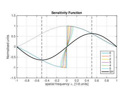
Figure 1: Pyramid 1D sensitivity plots for modulations $\{0,\cdots,5\}\lambda/D$ from (8) overlaid with Shack-Hartmann sensitivity when the discrete nature of the measurement is explicitly taken into account for a fair comparison between the PWFS and SH-WFS. Although the PWFS exhibits a slope-like and phase-like measurement regimes, this misconception is clarified in the text.

If instead we use developments by Fauvarque et al. (2019), then the PWFS OTF can be formulated as

$$\widetilde{\mathcal{W}}_{x}(\boldsymbol{\kappa})=\sqrt{|\widetilde{\mathcal{T}}_{x}(\boldsymbol{\kappa})\star\widetilde{\Pi}_{p}|^{2}}$$ (9)

where the function $\widetilde{\mathcal{T}}_{x}(\boldsymbol{\kappa})$ expands as

$$\widetilde{\mathcal{T}}_{x}(\boldsymbol{\kappa})=2i\left(H_{3}\star H_{2}\omega-H_{2}\star H_{3}\omega+H_{1}\star H_{4}\omega-H_{4}\star H_{1}\omega\right)$$ (10)

with $\omega$ a weighting function that characterizes the modulation signal, i.e., it encodes the normalised time spent on the modulation phase ${\boldsymbol{\theta}}({\mathbf{r}},t)$ over one integration frame. Provided it is expanded as a linear series of $n$ modes, ${\boldsymbol{\theta}}({\mathbf{r}},t)=\sum_{i=1}^{n}a_{i}(t)\mathcal{M}({\mathbf{r}})$ with $\mathcal{M}({\mathbf{r}})$ an orthonormal basis set, $\omega$ becomes

$$\omega=\widetilde{\mathcal{A}}\star\int_{t-T_{s}}^{T_{s}}a(t)\mathrm{d}t$$ (11)

where $\tilde{\mathcal{A}}$ is the Fourier-transformed aperture function.

The most common choice is tilt modulation for which case we have ${\boldsymbol{\theta}}({\mathbf{r}},t)=a_{1}(t)x+a_{2}(t)y$. If the modulation describes a perfect radially-symmetric ring, $a_{1}=a_{2}=$ and consequently, Eq. (11) becomes (Baddour (2011))

$$\omega=\text{\bf TF}^{-1}\left\{\mathcal{A}(\boldsymbol{\rho})\times J_{0}(\alpha\boldsymbol{\rho})\right\}$$ (12)

where $J_{0}(\alpha\boldsymbol{\rho})$ a Bessel function resulting from the Fourier transform of a (modulation) circle in the focal-plane. The relationship between modulation and tilt amplitude is $\alpha=\pi/4a$ in units of $\lambda/D$. This is the formulation that we will use in the remainder of this paper unless otherwise specified.

We note from Eq. (9) that the OTF is in fact the modulation transfer function (MTF) which provides the magnitude response of the optical system to harmonic functions of different spatial frequencies. The PWFS phase transfer function (PTF) is therefore null, a consequence of using intensity signals to measure a complex field.

A remarkable feature of this model is that the PWFS instantaneous response can now be understood and potentially used to estimate instantaneous optical gains (through the use of a complex-valued $\tilde{\mathcal{A}}$ function to a) optimise the run-time AO performance and b) estimate (and remove) quasi-static (pinned) speckles that limit the contrast achievable with high-contrast imagers.

2.3 A note on the nature of the PWFS signals

The dual behaviour of the modulated Pyramid sensor, acting as a slope-like sensor for low spatial frequencies and a phase-like sensor for high spatial frequencies is now well established yet it corresponds to a misconception. It stems from an erroneous analogy between the sensitivity of the pyramid and the nature of the measured signal initially stated in Vérinaud (2004) and represented in Fig. 1. Although for spatial-frequencies above the modulation $m\times\lambda/D$ the sensitivity is that of a phase sensor, the PWFS provides still a signal akin to the first spatial derivative of the phase (in the form of a Hilbert transform) with a frequency-dependent scaling at the origin of the misconception. Dubbing the PWFS measurements as "slopes” is, under this light, justified. Paradoxically, it is commonplace in the AO community.

In theory, for a large modulation the sensor will act more fully as a gradient sensor (with the correct frequency-dependent gains) and it may be possible to reconstruct from its measurements using previously derived Shack-Hartmann filters by Correia & Teixeira (2014a). One such successful albeit sub-optimal attempt can be found in Quirós-Pacheco et al. (2009).

2.4 Modelled vs. measured PWFS filter functions

Figure 2 shows the measured PWFS OTF using a full end-to-end physical optics model in Conan & Correia (2014) OOMAO implementing Eq. (1). The procedure is reminiscent of the "poke-matrix" in that we record the P-WF response to the complete set of complex-exponential functions in our basis set. It is compared to the model in Eq. (8) (which does not take into account the cross-terms for ease of presentation, although formulated in Conan (2003); Wang et al. (2010)) and in Eq. (9) for which one can clearly see the correct fit to the low-, high- and cross-term frequencies.

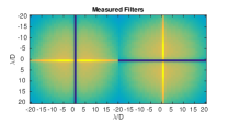
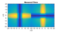
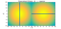
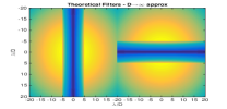
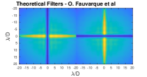
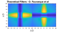
Figure 2: Comparison of measured with theoretical filters. Top: OOMAO-provided measurement (implementing (1)) . Mid: model from Eq. (8). Bottom: Model from Eq. 9. Left: modulation $1\lambda/D$. Right: $5\lambda/D$.

2.5 PWFS measurement noise model

In Feeney (2001) it is established that the effect of photon noise (yet not limited to) on the WFS measurements is such that

$$\sigma^{2}_{{\mathbf{s}}_{x},photon}=\sum_{q}\sigma^{2}_{i_{q}}\left(\frac{\partial{\mathbf{s}}_{x}}{\partial i_{q}}\right)^{2}$$ (13)

where $\sigma^{2}_{i_{q}}$ is the signal variance on the $q^{\text{th}}$ quadrant and

$${\mathbf{s}}_{x}=f(i_{1},i_{2},i_{3},i_{4})$$ (14)

from Eq. (3). The PWFS diffracted field gives rise to local intensity variations in the re-imaged pupil planes leading to $\sigma^{2}_{i_{q}}=\left\langle{i_{q}}\right\rangle$ under Poisson statistics where $\left\langle{\cdot}\right\rangle$ stands for ensemble-averaging. Besides, light falls outside the valid re-imaged pupils most prominently for low modulation cases, leading to a loss of SNR. Although one such noise model taking into account these features can be obtained straightforwardly, it lacks simplicity and practicality. We will assume for the sake of simplicity that the number of incident photons on each pixel is the same yielding

$$\sigma^{2}_{i_{q}}\approx n_{ph}/4$$ (15)

where $n_{ph}$ is the average number of photon detections on the PWFS.

Assuming the raw measurement

$${\mathbf{r}}_{x}=\frac{i_{q}+i_{n}}{i_{q}+i_{d}}$$ (16)

with $i_{d}$ and $i_{n}$ the shorthand for the other-than-$q$ quadrant intensities in the denominator and numerator respectively of Eq. (3). The measurement partial derivatives are readily found

$$\frac{\partial{\mathbf{s}}_{x}}{\partial i_{q}}=\frac{\partial{\mathbf{r}}_{x}}{\partial i_{q}}\frac{\partial{\mathbf{s}}_{x}}{\partial{\mathbf{r}}_{x}}=\frac{i_{q}+i_{d}+i_{q}+i_{n}}{(i_{q}+i_{d})^{2}}\frac{\partial{\mathbf{s}}_{x}}{\partial{\mathbf{r}}_{x}}$$ (17)

with $\frac{\partial{\mathbf{s}}_{x}}{\partial{\mathbf{r}}_{x}}$ playing the role of the pixel-dependent optical gain $g_{opt}$. For brevity and practical reasons, we assume it to be a scalar value. Using Eq. (15)

$$\frac{\partial{\mathbf{r}}_{x}}{\partial i_{q}}=\frac{4n_{ph}/4}{n_{ph}^{2}}=\frac{1}{n_{ph}}$$ (18)

Plugging (18) into (17) and then into (13), one finally gets

$$\sigma^{2}_{{\mathbf{s}}_{x},photon}=\left[4\frac{n_{ph}}{4}\left(\frac{1}{n_{ph}}\right)^{2}\left(\frac{\partial{\mathbf{s}}_{x}}{\partial{\mathbf{r}}_{x}}\right)^{2}\right]=\frac{g_{opt}^{2}}{n_{ph}}$$ (19)

For the read-out noise, following the same assumptions,

$$\sigma^{2}_{{\mathbf{s}}_{x},ron}=\sum_{q}\left(\frac{\partial{\mathbf{s}}_{x}}{\partial i_{q}}\right)^{2}$$ (20)

yielding

$$\sigma^{2}_{{\mathbf{s}}_{x},ron}=4g_{opt}^{2}\left(\frac{ron}{n_{ph}}\right)^{2}$$ (21)

where $ron$ is the average read-out-noise in photo-electrons per frame and per pixel.

Figure 3 compares the different models to physical-optics simulations, showing the great accuracy of the noise (photon and read) models (photon - $\sigma^{2}_{\eta}$ - and read-noise (50e-) - $\sigma^{2}_{ron}$. The multiple markers correspond to different modulations since the photo-electron count varies accordingly, albeit slightly.

Comparison to the SH-WFS: Since the PWFS has often been (wrongly) likened to the SH in quad-cell mode we provide the general expressions for the latter to enable the comparison offered in Fig. (3).

From Thomas et al. (2006)

$$\sigma^{2}=A\frac{1}{\bar{n}_{ph}}+B\left(\frac{ron}{\bar{n}_{ph}}\right)^{2}$$ (22)

with $A$ and $B$ a function of the algorithm used. $\bar{n}_{ph}$ is the number of photo-electrons/sub-aperture/frame and $ron$ is the effective read-out noise in photo-electrons rms.

For a quad-cell

$$A =\pi^{2}\kappa$$ (23)

$$B =4\pi^{2}\kappa^{2}$$ (24)

with $\kappa=1$ for a diffraction-limited spot.

We observe that using the quad-cell noise model from the SH-WFS applied to the PWFS leads to results different from those developed in Eq. (19) and Eq. (21).

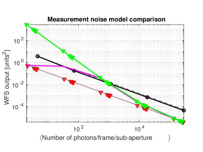
Figure 3: Illustrative example of noise models for the PWFS. Markers: theoretical from expressions in this section, no-markers: from physical-optics simulation models embedded in OOMAO (Conan & Correia (2014)). Red: photon-noise only. Green: photon+read noise. Magenta: physical-optics for photon+read noise. The saturation at low photon-count is the non-linear measurement regime manifesting (intensities are always positive). SH-WFS curves in black.

We show in Appendix the necessary steps to calculate the noise propagation expressed on an orthogonal basis of modes. Although for the SH-WFS the output variance can be assimilated to an OPD at the edges of the sub-apertures, we caution that the same cannot be achieved with the P-WFS on account of the nature of its measurement – see §2.3.

2.6 Considerations about VIS v. NIR WF Sensing

Photometric argument: Let the accuracy of the measurement be proportional to the diffraction $\lambda/D$ – i.e. take the optical gain in Eq. (17) to be inversely proportional to the angular size of PSF (its full-width at half maximum) that would be recorded at the vertex of the PWFS. A back of the envelope calculation tells us that it is more beneficial to use NIR wave-front sensing should the number of photons $n_{ph,NIR}>(\lambda_{NIR}/\lambda_{VIS})^{2}n_{ph,VIS}$ This standing, a factor $~{}4$ more photons is required in the NIR than in the VIS. Taking the case of SPHERE Fusco et al. (2016), the photometric budget for VIS and NIR detectors (CCD220 and Saphira respectively) coupled with the throughput of the whole instrument, we get $2\times 10^{9}ph/s/m^{2}$ at the central $\lambda_{VIS}=800\,nm$ whereas at $\lambda_{NIR}=1300\,nm$ we get $8\times 10^{9}\,ph/s/m^{2}$ with a G5 star. This seems to indicate that there is no huge gain in performing NIR WFSensing, avoiding further operational overheads of operating in the IR.

Morphological argument: As far as the PWFS is concerned, since we are not measuring the position of a PSF (as is the case of the SH-WFS), the previous argument is flawed, at least to the extent that the PWFS in normal operating regime features a mixed slope-like and phase-like sensitivities – §2.3 . Inasmuch as the relationship of the morphology of the PSF and its optical gain is non-linear, operating in the NIR is advantageous for the residuals at $\lambda_{NIR}$ are lesser allowing the PWFS to work closer to its linear regime. Conversely, in the VIS, the electric field is way more distorted (greater wave-front residuals), causing the PWFS to work in a "less linear” regime, therefore originating optical gain variations that are not fully compensated by an increase in photon collection from those sources (Bond et al. (2018)).

3 Analytical error budget evaluation

3.1 AO-induced OPD effects

Results in this section follow closely those in Correia et al. (2017). There we made a comprehensive presentation of how calculations of aniso-servo-lag, aliasing, measurement noise and fitting error can be conveniently evaluated using power-spectral densities in the spatial-frequency domain under temporally-filtered, closed-loop control.

Throughout this document the parameters in Table 1 are used by default.

Our goal is to evaluate the residual (piston-removed) phase variance, defined by

$$\sigma^{2}_{\text{Tot}}\triangleq\int\widetilde{\mathcal{P}}\left\langle\left|\widetilde{\boldsymbol{\varphi}}(\boldsymbol{\kappa})-{\widetilde{\boldsymbol{\varphi}}}^{\text{cor}}(\boldsymbol{\kappa})\right|^{2}\right\rangle\partial\boldsymbol{\kappa}$$ (25)

which is a function of $\{d,D,r_{0},L_{0},\sigma^{2}_{\eta}\}$, the actuator pitch, the telescope diameter, the atmosphere coherence length, the outer scale and the measurement noise variance.The piston-removal function is given by $\widetilde{\mathcal{P}}=\left[1-\left|\frac{2J_{1}(\pi\boldsymbol{\kappa}D)}{\pi\boldsymbol{\kappa}D}\right|^{2}\right]$with the term within the module the Fourier transform of a circular pupil function of diameter $D$.

In the remainder we suppose that the DM corrects entirely for the reconstructed phase, i.e. ${\widetilde{\boldsymbol{\varphi}}}^{\text{cor}}(\boldsymbol{\kappa})=\widehat{\widetilde{\boldsymbol{\varphi}}}(\boldsymbol{\kappa})=\widetilde{\mathcal{R}}\widetilde{\mathbf{s}}(\boldsymbol{\kappa})$ when the anti-folding filter is applied Correia & Teixeira (2014a)

Equation (25) is expanded using (7) yielding

$$\begin{split}\widetilde{\mathcal{P}}\left\langle{\left|\widetilde{\boldsymbol{\varphi}}(\boldsymbol{\kappa})-\widehat{\widetilde{\boldsymbol{\varphi}}}(\boldsymbol{\kappa})\right|^{2}}\right\rangle&=\widetilde{\mathcal{P}}\left\langle{\left|\tilde{\varepsilon}_{\perp}(\boldsymbol{\kappa})\right|^{2}}\right\rangle+\widetilde{\mathcal{P}}\left\langle{\left|\tilde{\varepsilon}_{||}(\boldsymbol{\kappa})\right|^{2}}\right\rangle\\ &=\left\langle{|\widetilde{\boldsymbol{\varphi}}_{\perp}|^{2}}\right\rangle\\ &\quad+\left|1-\widetilde{\mathcal{R}}\widetilde{\mathcal{W}}\right|^{2}\widetilde{\mathcal{P}}\left\langle{\widetilde{\boldsymbol{\varphi}}(\boldsymbol{\kappa})\widetilde{\boldsymbol{\varphi}}(\boldsymbol{\kappa})^{*}}\right\rangle\\ &\quad+\mathbf{W}_{\text{RA}}\\ &\quad+\left\langle{\widetilde{\mathcal{P}}\left|\widetilde{\mathcal{R}}\widetilde{\boldsymbol{\eta}}\right|^{2}}\right\rangle\end{split}$$ (26)

with $\left\langle{|\widetilde{\boldsymbol{\varphi}}_{\perp}|^{2}}\right\rangle$ the PSD of the fitting error (where we approximate $\widetilde{\mathcal{P}}(\boldsymbol{\kappa})=1$ for $|\boldsymbol{\kappa}|>1/(2d)$). The term

$$\left|1-\widetilde{\mathcal{R}}\widetilde{\mathcal{W}}\right|^{2}\widetilde{\mathcal{P}}\left\langle{\widetilde{\boldsymbol{\varphi}}(\boldsymbol{\kappa})\widetilde{\boldsymbol{\varphi}}(\boldsymbol{\kappa})^{*}}\right\rangle=\left|1-\widetilde{\mathcal{R}}\widetilde{\mathcal{W}}\right|^{2}\mathbf{W}_{\varphi}^{\prime}(\boldsymbol{\kappa})$$ (27)

is the PSD of the open-loop phase reconstruction error and

$$\mathbf{W}_{\text{RA}}=\widetilde{\mathcal{P}}\sum_{\mathbf{m}\neq 0}\left|\widetilde{\mathcal{R}}(\boldsymbol{\kappa})\widetilde{\mathcal{W}}(\boldsymbol{\kappa}+\mathbf{m}/d)\right|^{2}\mathbf{W}_{\varphi}(\boldsymbol{\kappa}+\mathbf{m}/d)$$ (28)

is the PSD of the reconstructed aliasing error. Finally

$$\mathbf{W}_{\eta}=\left\langle{\widetilde{\mathcal{P}}\left|\widetilde{\mathcal{R}}\widetilde{\boldsymbol{\eta}}\right|^{2}}\right\rangle$$ (29)

is the PSD of the propagated noise. This model can be (and was) further generalised to the closed-loop regime by Correia et al. (2017) when factoring in spatio-temporal functions characteristic of the loop filtering into Eq. ((26)).

Aliasing rejection: Figure 4 shows the propagated aliasing after least-squares wave-front reconstruction (Correia et al. (2017)) (i.e. with no temporal loop filtering). When comparing it to Fig. 9 in Vérinaud (2004), we note the general agreement. However, due to the two-dimensional reconstruction and the way x- and y- frequencies are mixed in the reconstructor’s denominator, a slab along $\kappa_{y}=0$ or $\kappa_{x}=0$ shows a damping for very low modulations. A cross-check on the likelihood of the result is also shown from the cuts along $\kappa_{x}=\kappa_{y}$ where all the propagated aliasing terms for both the pyramid WFS and the SH-WFS reach the same value at the edge of the control radius.

In either case the SH-WFS term is provided in black curves for comparison. Its amplitude is always greater than the one of the PWFS. The face-on patterns provide further insight into the propagated aliasing and its spatial distribution.

From Fig. (1) one hints at the fact that the amount of aliasing affecting either the PWFS or the SH is about the same. However, it is the propagation through the reconstructor that proves more beneficial with the PWFS.

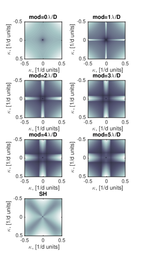
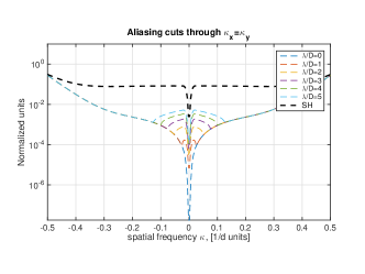
Figure 4: Propagated aliasing through LS reconstructor. Top: face-on patterns. Bottom: Slabs $\kappa_{y}=\kappa_{x}$.

Noise propagation: The noise is propagated through a LS reconstructor as shown in Fig. 5 (compare to Vérinaud (2004), Fig. 7). Here we are just showing a diagonal slab through the 2D noise propagation filter but the same comment applies to $\kappa_{x}=0$ of $\kappa_{y}=0$ slabs. As for the aliasing, the noise propagation is always lower for the pyramid WFS across all the spatial frequencies within the control radius.

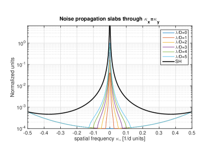
Figure 5: Propagated noise through LS reconstructor. Slab $\kappa_{y}=\kappa_{x}$.

3.2 Chromatic effects and scintillation

In addition to AO-induced residual OPD effects, now we consider additional limits to contrast due to chromatic effects and scintillation which generate both amplitude and OPD variations. Guyon (2005) and Fusco et al. (2006) provide quantification of such effects. We revisit those calculations and provide what we hope a more comprehensive taxonomy.

A wavelength-dependent index of refraction gives rise to 3 different errors (J.W.Hardy (1998)), to state,

1. angular dispersion due to the angle of incidence and refraction as the field propagates through the medium which can be seen as a cumulative version of Snell’s law over the vertical path

2. differential refraction error: chromatic path-length and amplitude errors for different wavelengths traversing the same path for they travel at different velocities creating a chromatic effect (dubbed correction chromatism by Fusco et al. (2006), term C6 in Guyon (2005))

3. dispersion displacement error caused by differential bending of wave-fronts at different wavelengths, causing rays to probe slightly different patches of turbulence resulting in an angular anisoplanatism-like error

To these adds scintillation plus OPD due to Fresnel propagation, even in the absence of chromatic refraction (Guyon (2005)) and despite the weak-turbulence regime (Roddier (1981)).

The first effect listed – angular dispersion – has no impact on contrast but solely on the angular positions of point sources on the focal plane; it is therefore disregarded in what ensues.

Now, let the index of refraction fluctuations for standard pressure and temperature from Edlén (1966) (later slightly adjusted by Owens (1967))

$$\Delta n(\lambda)=8.34213\times 10^{-5}+\frac{0.0240603}{130-\lambda^{-2}}+\frac{0.00015997}{38.9-\lambda^{-2}}$$ (30)

here taken to coincide with the refractivity index, i.e. $n=1+\Delta n$.

We assume the differential refraction error to be proportional to the ratio of fluctuations $\Delta n(\lambda_{1})/\Delta n(\lambda_{0})$ as suggested by Fusco et al. (2006) and not to the ratio of indices of refraction $n(\lambda_{1})/n(\lambda_{0})$ as was considered by Guyon (2005).

For the dispersion displacement error we follow Fusco et al. (2006) to compute an error PSD (both OPD and amplitude) considering anisoplanatic imaging with an angle

$$\theta=\Delta n(\lambda_{1})-\Delta n(\lambda_{0})tan(ZA)$$ (31)

where ZA is the zenith angle in radians.

Using standard expressions for Fresnel propagation (real and imaginary components) and differential chromaticity from Guyon (2005) we produced Fig. 6 with visible WFS and NIR imaging and Fig. 7 with both NIR WFS and imaging. As expected, amplitude effects are more pronounced when using much different wave-front sensing and imaging wavelengths.

In our implementation we do not consider interference between servo-lag OPD errors and scintillation although they give rise to tangible effects in post-coronagraphic images, in particular asymmetric halos in the AO correction region (commonly known as the butterfly due to its shape) caused by a combination of temporal delay and wind velocity (Cantalloube et al. (2018)).

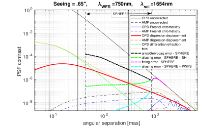
Figure 6: Post-coronagraphic PSF contrast curves including atmospheric dispersion effects and Fresnel propagation on both amplitude (AMP) and phase (optical path length - OPD) for a WFS in the VIS and a camera in the H-band. The maximum improvement is comprised between the black dashed curve (the anisoServoLag error) and the orange curve indicating the total of the non-AO limiting contrast terms. In the range {200 mas–1000 mas} the gap has an upper bound of a factor 10x. Vertical black lines indicate the correction band of Keck’s AO system (solid), SPHERE (dash) and the ELT (dotted).

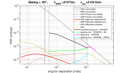
Figure 7: Post-coronagraphic PSF contrast curves including atmospheric dispersion effects and Fresnel propagation on both amplitude (AMP) and phase (optical path length - OPD) for both K-band WFSensing and imaging. The maximum improvement is comprised between the black dashed curve (the anisoServoLag error) and the orange curve indicating the total of the non-AO limiting contrast terms. In the range {50 mas–1000 mas} the gap reaches two orders of magnitude. Vertical black lines: see Fig. 6 caption.

We further notice (as done elsewhere by Guyon (2005); Fusco et al. (2006); Guyon (2018)) that the AO residuals – namely the servo-lag error - is by far the limiting factor. This provides compelling motivation for the investigation of predictive control approaches – see for instance Correia et al. (2017); Jared R. Males (2018); Massioni et al. (2015). We note also that the contrast estimates are well in-line with the results obtained with SPHERE on the VLT (Cantalloube et al. (2019); Vigan et al. (2019)) and Keck (Xuan et al. (2018)).

4 Wave-front reconstruction in the spatial-frequency domain

Having developed PWFS formulations and evaluated the AO-centric error budget from functions in the continuous spatial-frequency domain in previous sections, we devote this section to the real-time wave-front reconstruction from pyramid signals using discrete deconvolution-based processing as a natural extension of the preceding results. The default filter used here is the one recorded by measuring the PWFS response to the Fourier basis set with its physical-optics, diffractive model from Eq. (1).

The use of Fourier reconstruction has the potential to significantly increase the reconstruction speed (or otherwise lessen the computational burden), particularly for high-order systems such as those on Giant Segmented Mirror Telescopes (GSMTs) (Poyneer & Véran (2005); Correia et al. (2007)). On the other hand, and admitting that reconstruction speed in no longer of first priority due to the huge progress in real-time architectures over the last decade, we note that the use of spatial-frequencies extends the AO-correctable area by a factor $\pi/4$ with respect to orthonormal modes defined on a circular pupil that do not correct frequencies beyond $\kappa=\sqrt{\kappa_{x}^{2}+\kappa_{y}^{2}}>\frac{1}{2d}$ (although one such orthonormal basis could be formulated, to the authors knowledge it has not been used in the past). This ratio can even go higher when one considers the IWA of the coronagraph that is both affected by residual diffraction effects and by poor performance of the coronagraph.

Extensive development of Fourier reconstruction methods has focused on the Shack-Hartmann sensor, with compelling results - the most prominent being the Gemini Planet Imager Fourier Domain Reconstructor (Poyneer & Véran (2005)).

Advanced systems such as upgrades to existing telescopes (e.g. VLT’s SPHERE, Gemini’s GPI, Subaru’s ScExAO and Keck’s KPIC) and AO systems for future Giant Segmented Mirror Telescopes are likely to utilise the Pyramid wave-front sensor over the more commonly used Shack-Hartmann.

A discrete version of the analytic model provided in Eq. (8) can be applied to the real-time wave-front reconstruction from pyramid slope data. An initial attempt was made in Quirós-Pacheco et al. (2009) assuming a PWFS sensitivity function to be that of a SH-WFS (which of course is only valid in the highly modulated case). An implementation customized to the PWFS is presented in Shatokhina & Ramlau (2017) using 1-D reconstruction from PWFS signals in x and y directions and then averaging.

Here instead we follow on the footsteps of Bond et al. (2017) and on Fourier-domain implementations in Correia et al. (2007); Correia et al. (2008) that use jointly the x and y measurement data and take special care of the finite aperture edge effects and boundary conditions using circularity and divergence of the gradient field to ensure compatibility with the Fourier series. We find that this treatment is key to obtaining high levels of performance with minimal losses compared to the case that uses the full physical-optics PWFS model and SVD filtering to compute the reconstructor.

4.1 Discrete pyramid filter filters

We make use of a minimum-mean square minimisation criterion to find the following filters

$$\widehat{\tilde{\boldsymbol{\psi}}}=\mathbf{R}^{x}[k,l]\tilde{\mathbf{s}}_{x}+\mathbf{R}^{y}[k,l]\tilde{\mathbf{s}}_{y}$$ (32)

$$\widehat{{\boldsymbol{\psi}}}[k,l]=\left\{\begin{array}[]{ccc}0&\mbox{if $k,l=0$};\\ \hat{\mathbf{R}^{x}}[k,l]\tilde{{\mathbf{s}}}_{x}[k,l]+\hat{\mathbf{R}^{y}}[k,l]\tilde{{\mathbf{s}}}_{y}[k,l]&\mbox{otherwise}\end{array}\right.$$ (33)

It is straightforward to demonstrate that the MMSE (Wiener Filter) writes (Correia & Teixeira (2014a))

$$\widehat{\mathbf{{\boldsymbol{\psi}}}}=\frac{\mathbf{Q}_{x}^{*}\tilde{{\mathbf{s}}}_{x}+\mathbf{Q}_{y}^{*}\tilde{{\mathbf{s}}}_{y}}{|\mathbf{Q}_{x}|^{2}+|\mathbf{Q}_{y}|^{2}+\gamma\frac{\mathbf{W}_{n}}{\mathbf{W}_{\boldsymbol{\psi}}}}.$$ (34)

where $\mathbf{Q}$ is the discrete-version of the continuous model in Eq. (8) with the filters of the form

$$\hat{\mathbf{R}^{x}}[k,l]=\frac{\mathbf{Q}_{x}^{*}}{|\mathbf{Q}_{x}|^{2}+|\mathbf{Q}_{y}|^{2}+\gamma\frac{\mathbf{W}_{n}}{\mathbf{W}_{\boldsymbol{\psi}}}}$$ (35)

$$\hat{\mathbf{R}^{y}}[k,l]=\frac{\mathbf{Q}_{y}^{*}}{|\mathbf{Q}_{x}|^{2}+|\mathbf{Q}_{y}|^{2}+\gamma\frac{\mathbf{W}_{n}}{\mathbf{W}_{\boldsymbol{\psi}}}}$$ (36)

The least-squares solution is easily obtained by taking $\gamma=0$.

The priors $\mathbf{W}_{n}$ and $\mathbf{W}_{\boldsymbol{\psi}}=0.49r_{0}^{-5/3}\left\{(2\pi)^{2}\left[f_{x}^{2}+f_{y}^{2}+(1/L_{0})^{2}\right]\right\}^{-11/6}$, are the spatial PSDs of the noise and the phase. The noise is assumed white and uncorrelated, thus constant over all the frequencies, i. e. $\mathbf{W}_{n}\propto k\in\Re$. An anti-aliasing Wiener filtering solution is developed in Correia & Teixeira (2014b) by suitably modifying the whiteness of the noise. A further scalar factor $\gamma$ is introduced to properly weigh the priors term to account for other unknown system parameters.

5 Limiting performance and contrast

We are now in a position to apply the results from the preceding sections to representative cases of high-contrast imagers. In this section we investigate (analytically & with Monte-Carlo models) the performance for our simulated system as a function of exposure time, modulation and guide-star magnitude In so doing we revisit the work of Vérinaud (2004) and extend it to the 2-dimensional case.

Further parameters can be found on Table 1.

Table 1: Default simulation parameters. The turbulence model represents median Paranal conditions. Bold represents the nominal conditions.

Telescope
D	8.0 m
throughput	50%
Guide-star
zenith angle	0-60 deg
magnitude	0-12
Atmosphere
$r_{0}$	15 cm
$L_{0}$	25 m
Fractional $r_{0}$	[53.28;1.45;3.5;9.57;10.83;
	4.37;6.58;3.71;6.71]/100
Altitudes	[0.042;0.140;0.281;0.562;1.125;
	2.25;4.5;9;18] km
wind speeds	[15;13;13;9;9;
	15;25;40;21] m/s
wind direction	[38;34;54;42;57;
	48;-102;-83;-77]*$\pi$/180 deg
Wave-front Sensor
Order	40$\times$40
RON	1 e-
$n_{pix}$	4
$f_{sample}=1/T_{s}$	0.1–1–5 kHz
modulation $m$	0–2–6 $\lambda/D$
$\lambda_{WFS}$	0.64–1.65–2.2 $\mu$m
Centroiding algorithm	thresholded CoG
DM
Order	41$\times$41
AO loop
pure delay	$\tau_{\mathsf{lag}}=$1 ms
loop gain	$g=\{0.01,\cdots,0.5\}$
Imaging Wavelength
$\lambda_{im}$	0.75–1.65–2.2 $\mu$m

5.1 $\lambda_{im}$=NIR, $\lambda_{WFS}$=VIS in imaging mode

As an example of the analytic error breakdown and reconstruction accuracy, Fig. 8 compares the limiting performance expected from a visible PWFS and SH-WFS on a 8 m-class telescope as a function of guide-star magnitude and AO loop sampling frequency. Using developments in Sect. 4 we over-plot (circle and triangle markers) the results of Monte-Carlo simulations performed under Conan & Correia (2014)’s OOMAO.

It is interesting to note that for bright guide-stars there is only a slight advantage for the pyramid. Looking at the full 2-D PSFs would further give insight into differences between these two wave-front sensors that the SR is incapable of showing.

On the faint star end, the pyramid is at its best. The lower noise propagation, i.e. increased sensitivity, makes it push the limiting magnitude by roughly two stellar magnitudes. Whereas the SH drop-off knee is around magnitude 12, the pyramid ensures good performances down to magnitude 14. At magnitude 15, the pyramid still achieves $30\%$ SR, a pretty high value.

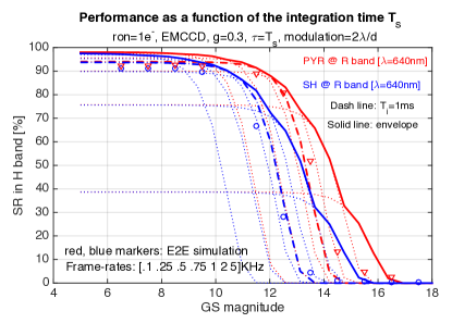
Figure 8: Performance comparison between the analytic and the Monte-Carlo models, both available from OOMAO. Dashed curves indicate the 1kHz frame-rate case to be compared to the results (markers only) of the Monte-Carlo simulations. In the latter the PWFS optical gain are compensated for by adjusting a single scalar gain which in our opinion is at the origin of the slight drop in performance on the bright star end.

5.2 $\lambda_{im}$=VIS, $\lambda_{WFS}$=NIR in imaging mode

We can likewise explore the performance at visible wavelengths of a pyramid-based high-contrast AO system. The motivation is two-fold: i) provide performance in a parameter space complementary to that of space-borne and ground-based high-resolution spectrographs used for the indirect detection and characterisation of extra-solar planets and disks and ii) guide on IR stars and brown-dwarfs, the latter relatively fainter at visible wavelengths yet likely to host planetary systems as well.

Figure 9 shows the performance in the I-band ($\lambda_{im}$=850 nm) when the sensing is done in H-band ($\lambda_{WFS}$=1650 nm) as a function of guide-star magnitude, frame-rate and pyramid modulation. We have considered fast IR detectors with sub-electron noise providing for fast reading. We can observe the huge impact of running at higher frame-rates, with the performance increasing from 60% at 500 Hz to 80+% at 5000 Hz. This is strong indication that servo-lag error is the dominant factor.

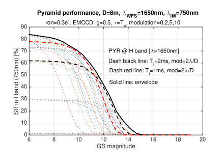
Figure 9: Performance expected at visible wavelengths by a PWFS system.

5.3 Integral vs. distributed control in coronagraphic mode

In an attempt to minimise residual AO errors after correction, the results that follow build on the predictive capabilities of distributed Kalman filters with the formulation presented in Correia et al. (2017).

We first investigate the net effect of using predictive control over single-gain integral control in Fig. 10 for a SH-based high-contrast imager. There, we plot the contrast improvement as a ratio (negative values, since we are using a log scale) or a degradation (positive values). The 2D nature of these plots adds to the limiting contrast curves in Fig. 6 and 7 which radially symmetric in nature; we can observe on the bright star end that contrast improvements can surpass the factor 10x at small separations (typically below 5 $\lambda/D$) and in certain wind-dependent directions.

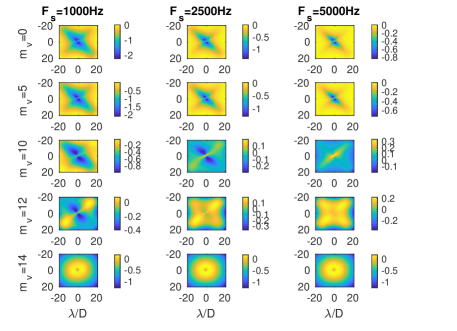
Figure 10: Contrast ratio map (log scale) as a function of the frame-rate and stellar magnitude for a SH with a LS reconstructor and integral controller versus a DKF controller.

When a PWFS is employed, then the potential contrast improvement increases as shown in Fig. 11 in both depth and extent.

For a magnitude 0 star, a combination of pyramid+DKF can clean up the AO control region almost entirely, resulting in an extended zone with up to two orders of magnitude contrast ratio improvement. This happens on account of the almost complete removal of servo-lag (typically $\in\pm 5\lambda/D$) and aliasing terms (closer to the AO correction edges). As we move towards higher frame-rates, the improvement brought upon by the DKF is lesser for the servo-lag error is smaller (as in Fig. 10).

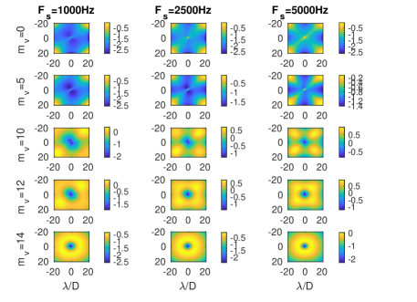
Figure 11: Contrast ratio map (log scale) as a function of the frame-rate and stellar magnitude for a SH with a LS reconstructor and integral controller versus a PWFS with a DKF controller.

In real observations the presence of quasi-static speckles can limit the contrast figures provided. With the possibility offered by the models in §2 to estimate instantaneously the PWFS optical gains, we left for the interested reader the exploration of pushing the contrast further when using noiseless detectors (or very low read noise) from which high-quality short-exposure images can be collected with custom post-processing techniques ingrained with knowledge of the variability of those optical gains.

6 Conclusion

We have shown the performance limits of the pyramid wave-front sensor for both imaging and high-contrast applications. For that we produced an AO-centric error breakdown using a practical, convolution-based PWFS model in the spatial-frequency domain (developed in Fauvarque et al. (2019)) featuring some highly desirable properties

• its meta-intensity linear model (from which the slopes-maps are computed as linear combinations) represents to a broader extent the diffractive nature the PWFS optic.

• this model can be generalised to finite pupils, coherent and incoherent recombination of light resulting from overlapping and non-overlapping re-imaged pupils respectively, extended-objects, and off-line optical gains retrieval

Our calculations back the generally accepted result whereby the PWFS extends by up to two stellar magnitudes the limiting WFS magnitude allowing for a larger sky-coverage (not quantified here)

On existing high-contrast imagers mounted on 10 m-class telescopes with visible or near-infrared PWFS under median Paranal turbulence conditions outlined in 1, we show a contrast improvement (limited by chromatic and scintillation effects) of 2x-10x by replacing the wave-front sensor alone at large separations close to the AO control radius where aliasing dominates, and factors in excess of 10x by coupling distributed control with the PWFS over most of the AO control region, from small separations starting with the Inner Working Angle of typically 1-2 $\lambda/D$ to the AO correction edge.

Appendix A Noise propagation expressed on an orthonormal basis of modes

Results in this section follow closely the approach of Rigaut & Gendron (1992). The propagated noise covariance matrix on a predefined basis set of modes is defined as

$$\boldsymbol{\Sigma}_{m}=\left\langle{\mathbf{m}\mathbf{m}^{\mathsf{T}}}\right\rangle$$ (37)

with the reconstructed modal coefficient vector $\mathbf{m}$

$$\mathbf{m}=\mathbf{G}^{\dagger}{\boldsymbol{\eta}}$$ (38)

where ${\boldsymbol{\eta}}$ is a vector WFS measurement signals, $\mathbf{G}^{\dagger}=(\mathbf{G}\mathbf{G}^{\mathsf{T}})^{-1}\mathbf{G}^{\mathsf{T}}$ and $\mathbf{G}$ is the system interaction matrix ${\mathbf{s}}=\mathbf{G}{\boldsymbol{\psi}}$ containing the responses of the WFS to each mode in $\mathbf{m}_{i}$ of ${\boldsymbol{\psi}}$. For the PWFS this is the covariance function that needs be evaluated, i.e.

$$\boldsymbol{\Sigma}_{m} =\mathbf{G}^{\dagger}\left\langle{{\boldsymbol{\eta}}{\boldsymbol{\eta}}^{\mathsf{T}}}\right\rangle\mathbf{G}^{\dagger}$$ (39)

and $\left\langle{{\boldsymbol{\eta}}{\boldsymbol{\eta}}^{\mathsf{T}}}\right\rangle$ provided in Eq. (19) and Eq. (21).

For linear WFSs a simplification applies. If we consider now a measurement of pure noise which is assumed of constant variance $\sigma^{2}_{\eta}$ across the pupil then the noise propagated is

$$\boldsymbol{\Sigma}_{m} =\mathbf{G}^{\dagger}\left\langle{{\mathbf{s}}{\mathbf{s}}^{\mathsf{T}}}\right\rangle\mathbf{G}^{\dagger}$$ (40)

$$=(\mathbf{G}\mathbf{G}^{\mathsf{T}})^{-1}\sigma^{2}_{\eta}$$ (41)

provided that $\left\langle{{\mathbf{s}}{\mathbf{s}}^{\mathsf{T}}}\right\rangle=\mathbf{I}\sigma^{2}_{\eta}$. Using SVD decomposition

$$[\mathcal{U}\mathcal{S}\mathcal{V}^{\mathsf{T}}]=svd(\mathbf{G})$$ (42)

where $\mathcal{S}=diag(\beta_{ii})$ is a diagonal matrix with the singular values in it.

One can likewise write

$$(\mathbf{G}\mathbf{G}^{\mathsf{T}})^{-1}=\left(\mathcal{V}\mathcal{S}^{\mathsf{T}}\mathcal{U}^{\mathsf{T}}\mathcal{U}\mathcal{S}\mathcal{V}^{\mathsf{T}}\right)^{-1}$$ (43)

Using the equalities $\mathcal{U}^{\mathsf{T}}=\mathcal{U}^{-1}$ and $\mathcal{V}^{\mathsf{T}}=\mathcal{V}^{-1}$ one gets

$$(\mathbf{G}\mathbf{G}^{\mathsf{T}})^{-1}=\mathcal{V}\mathcal{S}^{-\mathsf{T}}\mathcal{S}^{-1}\mathcal{V}^{\mathsf{T}}$$ (44)

from which the $k^{th}$ element of the diagonal writes

$$\sigma^{2}_{k} =\sum_{i}\mathcal{V}_{k,i}\frac{1}{\beta_{ii}^{2}}\mathcal{V}_{ik}^{\mathsf{T}}$$ (45)

$$=\sum_{i}\mathcal{V}_{ki}\frac{1}{\beta_{ii}^{2}}\mathcal{V}_{ki}$$ (46)

$$=\sum_{i}\frac{\mathcal{V}_{ki}^{2}}{\beta_{ii}^{2}}$$ (47)

which is a more straightforward demonstration but otherwise equivalent to that of Feeney (2001).

We caution the reader however that the PWFS noise propagation coefficients cannot be quoted in units of angle-on-sky since its measurements, unlike the SH-WFS, are not straight wave-front gradients (or slopes).

Appendix B Variations around WFS and controller choices

Figures 12, 13 and 14 depict the contrast ratios obtained as a function of the stellar magnitude and frame-rate for the different choices of WFS and controller (for a constant pure loop delay of 3 ms).

The remainder of the figures show different combinations of controllers and WFS.

Figure 12 shows the contrast improvements by increasing the frame rate for a SH-based system with the DKF controller. Gains are observed in a butterfly shaped region for brighter stars and it vanished as noise becomes the dominant factor for fainter stars.

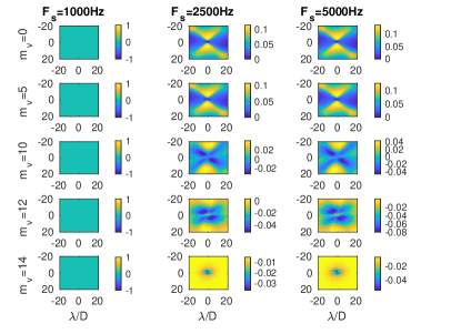
Figure 12: Contrast ratio map as a function of the frame-rate and stellar magnitude for a SH with a DKF controller.

If we now look into the contrast gains of just replacing the SH by a PWFS, but keeping the controller we find results in Fig. 13. It seems that only a poor improvement is achieved regardless of the magnitude and frame-rate chosen.

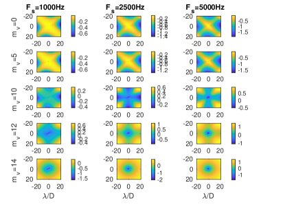
Figure 13: Contrast ratio map as a function of the frame-rate and stellar magnitude for a PWFS versus a SH-based system both with a LS reconstructor and integral controller.

Finally, Fig. 14 shows the improvement of increasing the frame-rate with the SH and integral controller. Compared to Fig. 10 the contrast improvements are not nearly as spectacular since the controller adds no predictive knowledge to the wave-front estimation in order to further improve contrast as small separations.

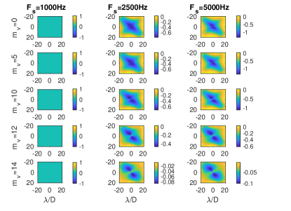
Figure 14: Contrast ratio map as a function of the frame-rate and stellar magnitude for a SH with a DKF controller.

References

- Baddour (2011) Baddour N., 2011, Advances in Imaging and Electron Physics - ADV IMAG ELECTRON PHYS, 165, 1
- Beuzit et al. (2019) Beuzit J. L., et al., 2019, A&A, 631, A155
- Bond et al. (2016) Bond C. Z., El Hadi K., Sauvage J. F., Correia C., Fauvarque O., Rabaud D., Neichel B., Fusco T., 2016, in AO4ELT-IIII.
- Bond et al. (2017) Bond C. Z., Correia C. M., Sauvage J.-F., Neichel B., Fusco T., 2017, Opt. Express, 25, 11452
- Bond et al. (2018) Bond C. Z., et al., 2018, in Proc. SPIE. p. 107031Z, doi:10.1117/12.2314121
- Cantalloube et al. (2018) Cantalloube F., et al., 2018, Astronomy & Astrophysics, 620, L10
- Cantalloube et al. (2019) Cantalloube F., Dohlen K., Milli J., Brandner W., Vigan A., 2019, The Messenger, 176, 25
- Chew et al. (2006) Chew T. Y., Clare R. M., Lane R. G., 2006, Optics Communications, 268, 189
- Conan (2003) Conan R., 2003, Technical report, Fourier optics and distribution theory applied to pyramid wavefront sensors. LAOG/ONERA
- Conan & Correia (2014) Conan R., Correia C., 2014, in SPIE 9148.
- Correia & Teixeira (2014a) Correia C. M., Teixeira J., 2014a, Journal of the Optical Society of America A, 31, 2763
- Correia & Teixeira (2014b) Correia C. M., Teixeira J., 2014b, Journal of the Optical Society of America A, 31, 2763
- Correia et al. (2007) Correia C., Conan J. M., Kulcsár C., Raynaud H. F., Petit C., Fusco T., 2007, in Bouvier J., Chalabaev A., Charbonnel C., eds, SF2A-2007: Proceedings of the Annual meeting of the French Society of Astronomy and Astrophysics. p. 25
- Correia et al. (2008) Correia C., Kulcsar C., Conan J.-M., Raynaud H.-F., 2008, in Hubin N., Max C. E., Wizinowich P. L., eds, Vol. 7015, Proc. of the SPIE. SPIE, p. 701551, doi:10.1117/12.788455, http://link.aip.org/link/?PSI/7015/701551/1
- Correia et al. (2017) Correia C. M., Bond C. Z., Sauvage J.-F., Fusco T., Conan R., Wizinowich P. L., 2017, J. Opt. Soc. Am. A, 34, 1877
- Deo et al. (2018) Deo V., Gendron É., Rousset G., Vidal F., Buey T., 2018, in Society of Photo-Optical Instrumentation Engineers (SPIE) Conference Series. p. 1070320, doi:10.1117/12.2311631
- Edlén (1966) Edlén B., 1966, Metrologia, 2, 71
- Esposito et al. (2015) Esposito S., Pinna E., Puglisi A., Agapito G., Veran J. P., Herriot G., 2015, in Adaptive Optics for Extremely Large Telescopes IV (AO4ELT4). p. E36
- Fauvarque (2017) Fauvarque O., 2017, PhD thesis, Aix-Marseille Univ
- Fauvarque et al. (2015) Fauvarque O., Neichel B., Fusco T., Sauvage J.-F., 2015, Optics Letters, 40, 3528
- Fauvarque et al. (2017) Fauvarque O., Neichel B., Fusco T., Sauvage J.-F., Girault O., 2017, Journal of Astronomical Telescopes, Instruments, and Systems, 3, 019001
- Fauvarque et al. (2019) Fauvarque O., Janin-Potiron P., Correia C., Brule Y., Neichel B., Chambouleyron V., Sauvage J.-F., Fusco T., 2019, arXiv e-prints, p. arXiv:1902.05440
- Feeney (2001) Feeney O. A., 2001, Technical report, Theory and Laboratory Characterisation of Novel Wavefront Sensor for Adaptive Optics Systems. National University of Ireland, Galway
- Fusco et al. (2006) Fusco T., et al., 2006, Optics Express, 14, 7515
- Fusco et al. (2016) Fusco T., et al., 2016, in Adaptive Optics Systems V. p. 99090U, doi:10.1117/12.2233319
- Guyon (2005) Guyon O., 2005, The Astrophysical Journal, 629, 592
- Guyon (2018) Guyon O., 2018, Annual Review of Astronomy and Astrophysics, 56, 315
- J.W.Hardy (1998) J.W.Hardy 1998, Adaptive Optics for Astronomical Telescopes. Oxford, New York
- Jared R. Males (2018) Jared R. Males O. G., 2018, Journal of Astronomical Telescopes, Instruments, and Systems, 4, 4
- Korkiakoski et al. (2007) Korkiakoski V., Vérinaud C., Louarn M. L., Conan R., 2007, Appl. Opt., 46, 6176
- LeDue et al. (2009) LeDue J., Jolissaint L., Véran J.-P., Bradley C., 2009, Opt. Express, 17, 7186
- Linfoot (1948) Linfoot E. H., 1948, MNRAS, 108, 428
- Macintosh et al. (2018) Macintosh B., et al., 2018, in Proc. SPIE. p. 107030K (arXiv:1807.07146), doi:10.1117/12.2314253
- Massioni et al. (2015) Massioni P., Gilles L., Ellerbroek B., 2015, J. Opt. Soc. Am. A, 32, 2353
- Mawet et al. (2012) Mawet D., et al., 2012, Review of small-angle coronagraphic techniques in the wake of ground-based second-generation adaptive optics systems. p. 844204, doi:10.1117/12.927245
- Mawet et al. (2014) Mawet D., et al., 2014, ApJ, 792, 97
- Mawet et al. (2016) Mawet D., et al., 2016, Keck Planet Imager and Characterizer: concept and phased implementation. p. 99090D, doi:10.1117/12.2233658
- Mouillet et al. (2018) Mouillet D., et al., 2018, in Proc. SPIE. p. 107031Q, doi:10.1117/12.2313277
- Oppenheim & Schafer (1999) Oppenheim A. V., Schafer R. W., 1999, Discrete-time signal processing, 2nd edn. Prentice-Hall,Inc.
- Owens (1967) Owens J. C., 1967, Appl. Opt., 6, 51
- Poyneer & Véran (2005) Poyneer L. A., Véran J.-P., 2005, Journal of the Optical Society of America A, 22, 1515
- Quirós-Pacheco et al. (2009) Quirós-Pacheco F., Correia C., Esposito S., 2009, in Y. Clénet J.-M. Conan T. F., Rousset G., eds, 1st AO4ELT Conference - Adaptative Optics for Extremely Large Telescopes proceedings. No. 07005. EDP Sciences
- Ragazzoni (1996) Ragazzoni R., 1996, Journal of Modern Optics, 43, 289
- Rigaut & Gendron (1992) Rigaut F., Gendron E., 1992, Astronomy and Astrophysics, 261, 677
- Roddier (1981) Roddier F., 1981, The effects of atmospherical turbulence in optical astronomy. pp 281–376
- Shatokhina & Ramlau (2017) Shatokhina I., Ramlau R., 2017, Appl. Opt., 56, 6381
- Shatokhina et al. (2013) Shatokhina I., Obereder A., Rosensteiner M., Ramlau R., 2013, Appl. Opt., 52, 2640
- Snik et al. (2018) Snik F., et al., 2018, in Proc. SPIE. p. 107062L (arXiv:1807.07100), doi:10.1117/12.2313957
- Thomas et al. (2006) Thomas S., Fusco T., Tokovinin A., Nicolle M., Michau V., Rousset G., 2006, MNRAS, 371, 323
- Vérinaud (2004) Vérinaud C., 2004, Optics Communications, 233, 27
- Vérinaud et al. (2005) Vérinaud C., Le Louarn M., Korkiakoski V., Carbillet M., 2005, Monthly Notices of the Royal Astronomical Society, 357, L26
- Vigan et al. (2019) Vigan A., et al., 2019, A&A, 629, A11
- Wang et al. (2010) Wang J., Bai F., Ning Y., Huang L., Wang S., 2010, Opt. Express, 18, 27534
- Xuan et al. (2018) Xuan W. J., et al., 2018, AJ, 156, 156