Observation of strong two-electron–one-photon transitions in few-electron ions

Abstract

We resonantly excite the $K$ series of O⁵⁺ and O⁶⁺ up to principal quantum number $n=11$ with monochromatic x rays, producing $K$-shell holes, and observe their relaxation by soft-x-ray emission. Some photoabsorption resonances of O⁵⁺ reveal strong two-electron–one-photon (TEOP) transitions. We find that for the $[(1s\,2s)_{1}\,5p_{3/2}]_{3/2;1/2}$ states, TEOP relaxation is by far stronger than the radiative decay and competes with the usually much faster Auger decay path. This enhanced TEOP decay arises from a strong correlation with the near-degenerate upper states $[(1s\,2p_{3/2})_{1}\,4s]_{3/2;1/2}$ of a Li-like satellite blend of the He-like $K\alpha$ transition. Even in three-electron systems, TEOP transitions can play a dominant role, and the present results should guide further research on the ubiquitous and abundant many-electron ions where electronic energy degeneracies are far more common and configuration mixing is stronger.
   
DOI: 10.1103/PhysRevA.102.052831

I Introduction

In hot astrophysical plasmas, the most common elements, hydrogen and helium, are fully ionized, and only those with higher nuclear charge can keep some bound electrons, appearing as highly charged ions (HCIs) Beiersdorfer (2003). The widths, Doppler shifts and relative intensities of their characteristic lines are recorded by x-ray observatories and analyzed for plasma diagnostics, relying not only on tabulated calculations but also on more scarce laboratory data. To fully exploit the data of current and upcoming high-resolution x-ray missions such as XRISM Tashiro et al. (2018) and Athena Barret et al. (2016), more accurate laboratory tests of the atomic models used in astrophysics are needed Beiersdorfer (2003); Hell et al. (2020). Light elements such as carbon, nitrogen, and the oxygen studied here abundantly appear as HCIs over a broad range of temperatures and can thus serve as unique spectroscopic probes of, e.g., the warm-hot intergalactic medium (WHIM), which is critical to a complete census of baryonic matter in the universe Simcoe et al. (2002); Nicastro et al. (2018); Gatuzz et al. (2019). It is important to have knowledge of both the photoabsorption cross sections and the various decay channels that govern the fluorescence yield and the ionization balance in plasmas. After x-ray absorption takes place, the most common relaxation processes are direct radiative decay and autoionization. However, even in few-electron systems, more complex processes and multi-electron transitions also compete with them. Including such mechanisms in models is computationally intensive, and hence laboratory data are needed to guide those efforts Kallman and Palmeri (2007).

Many-electron processes are intensively studied in both theory and experiment, and there is a plethora of recent examples on various subjects: multiple photodetachment of anions (see e. g., Gorczyca (2004); Schippers et al. (2016a); Müller et al. (2018); Perry-Sassmannshausen et al. (2020) and references therein); photoionization of atoms and ions West (2001); Kjeldsen (2006); Bizau et al. (2015); Berrah et al. (2004); Gharaibeh et al. (2011) near inner-shell absorption edges Levin and Armen (2004); Kabachnik et al. (2007); Southworth et al. (2019); Ma et al. (2017); and higher-order relaxation processes Dunford et al. (2004). This also applies to ions (see e. g., Schippers et al. (2016b); Müller et al. (2017), HCI Blancard et al. (2018); Simon et al. (2010); Steinbrügge et al. (2015); Bliman et al. (1989); Tawara and Richard (2002); Kato et al. (2006) and their interactions with free-electron lasers Young et al. (2010); Buth et al. (2018). Photorecombination also triggers multi-electronic excitations through resonant dielectronic Beiersdorfer et al. (1992); Nakamura et al. (2008); Shah et al. (2015), trielectronic and quadruelectronic processes Schnell et al. (2003); Beilmann et al. (2011); Shah et al. (2016). The complexity of interelectronic correlations already within the $L$ shell Drake et al. (1999); Bizau et al. (2015); Liu et al. (2018); Zaytsev et al. (2019) forces theoreticians to use approximations with uncertainties that are hard to benchmark in the absence of laboratory data. As an example, the crucial determination of the cosmic abundance and column-density of O⁵⁺ in the WHIM suffers from large theoretical uncertainties Behar et al. (2001); McLaughlin et al. (2016); Gatuzz et al. (2019); Mathur et al. (2017).

Here, we report on resonant excitation of the $K$ series of He-like and Li-like oxygen ions between 570 and 750 eV using monoenergetic soft x rays. We detect their fluorescence-photon yield and energy as a function of the incident photon energy, and observe surprisingly strong and sometimes dominating two-electron–one-photon (TEOP) transitions in Li-like oxygen.

II Experimental setup

Our experiment was conducted at the variable-polarization XUV beamline P04 Viefhaus et al. (2013) of the PETRA III synchrotron facility with a portable electron beam ion trap (EBIT), PolarX Micke et al. (2018) (see Fig. 1). Molecular oxygen was injected into the EBIT, dissociated and successively ionized yielding a large He-like O⁶⁺ population and a small Li-like O⁵⁺ fraction. These HCI are radially trapped by the electron beam (here 3 mA, to reduce ion heating), and axially confined within a potential well formed by making the central drift tube slightly more negative than the adjacent ones. With an electron-beam energy of $\sim$200 eV just above the Li-like ionization threshold, we produce He-like O⁶⁺, but stay below the excitation threshold of $K\alpha$ or higher $Kn$ series transitions. This ensures a low-background measurement of the $K$ series fluorescence by a silicon-drift detector (SDD) mounted side-on above the central drift tube where the ions are confined.

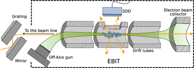
Figure 1: Schematic of PolarX EBIT Micke et al. (2018). An electron beam from an off-axis gun is focused by a magnetic field and passes through drift tubes, where it generates and traps highly charged ions before reaching a collector electrode. A monochromatic photon beam enters axially and excites the trapped ions. The energies of fluorescence photons are recorded by a silicon-drift detector (SDD), similarly to Kühn et al. (2020).

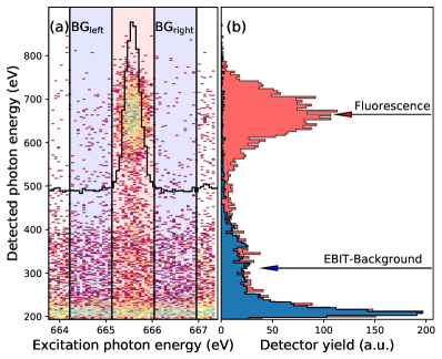
Figure 2: a) Fluorescence yield (recorded by the SDD) of He-like O⁶⁺ $K_{\beta}$ under excitation with $663\text{\,}\mathrm{-}$$668\text{\,}\mathrm{eV}$ photons ($x$ axis) versus fluorescence-photon energy ($y$ axis), and (black curve) projection of the photon yield onto $x$. b) Projections onto the $y$ axis of on/off resonance slices (red/blue histograms). The off-projection is used for subtraction of electron-induced background and SDD-noise.

The P04 beamline is equipped with an APPLE-II undulator covering the photon energy range $250\text{\,}\mathrm{-}$- $3000\text{\,}\mathrm{eV}$, and a grating monochromator ($1200\text{\,}\mathrm{l}$ines/mm) providing circularly polarized light at a resolving power of more than ${10}^{4}\text{\,}$ Viefhaus et al. (2013). Expected long-time drifts of the monochromator recommended for this overview measurement a fast-scan mode lasting less than one hour, forcing the use of a wide slit (200 $\mu$m) for better statistics. This gives us a photon flux on the order of $10^{12}$ photons/s at a moderate resolving power. Nonetheless, we could determine excitation energies with a relative uncertainty of $\Delta E/E\approx 10^{-5}$. For this, we digitize the SDD-energy signal ($y$ axis) for each photon-detection event while continuously scanning the monochromator, i. e., the incident photon energy ($x$ axis), obtaining a two-dimensional fluorescence histogram (Fig. 3a). To remove background events due to electron recombination, we subtract at each resonance the off-resonance mean count rate from the on-resonance signal (see an example in Fig. 2). Then, we project the region of interest containing the resonance onto both axes, and fit Gaussians with a full widths at half maximum of order of $350\text{\,}\mathrm{meV}$ ($x$ axis) and order of $100\text{\,}\mathrm{eV}$ ($y$ axis) to those projections.

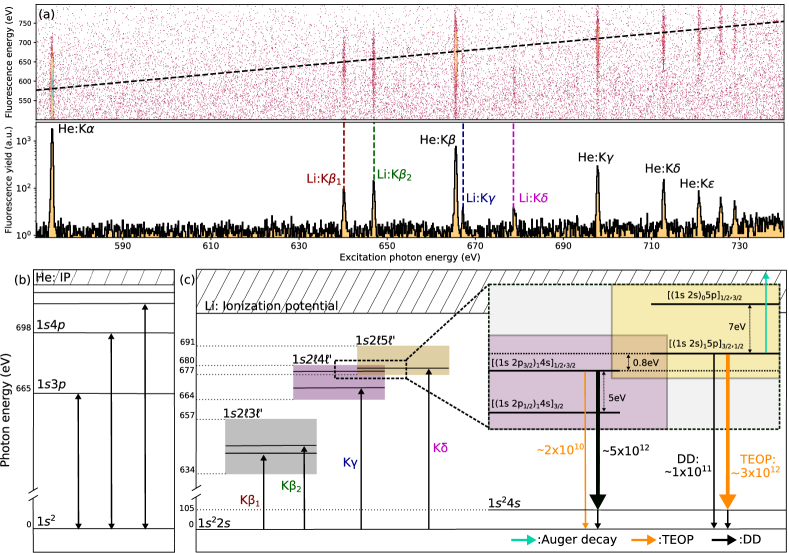
Figure 3: a) Shown on top is a histogram of events registered with the SDD: fluorescence photon energy ($y$ axis) versus excitation photon energy ($x$ axis). The dashed diagonal line indicates elastic channels, with excitation and the fluorescence photon at equal energies. Shown on the bottom is fluorescence from resonantly photoexcited He-like O⁶⁺ and Li-like O⁵⁺, labeled in black and in color, respectively. b) He-like and c) Li-like level diagrams. Configuration mixing of the upper levels of K$\delta$ causes a predominance of the TEOP process over both the elastic direct decay to the ground state and the Auger channels. Rates are in units of s^-1.

III MEASUREMENT OF PHOTOEXCITATION ENERGIES

A monochromator scan from $570\text{\,}\mathrm{eV}$ to $740\text{\,}\mathrm{eV}$ at $500\text{\,}\mathrm{meV}\text{\,}{\mathrm{s}}^{-1}$ resolved the core excited $K$ series of He-like oxygen up to $K\kappa$, as well as several other weaker Li-like resonances (Fig. 3). After determining their centroid positions (see Fig. 3a), we assign to the six transitions $K\alpha$ up to $K\zeta$ (identified on the approximately calibrated $x$ axis for the incident photon-energy in Fig. 3) energies taken from accurate calculations by Yerokhin and Surzhykov (2019) with uncertainties on the order of $0.5\text{\,}\mathrm{meV}$ and determine the final monochromator-dispersion curve with a linear fit. Its confidence interval is basically dominated by the order of 20-meV statistical uncertainties of the individual transitions in our fast overview scan. By extrapolating the dispersion curve we obtain the excitation energies of the $K\eta$, $K\theta$, $K\iota$ and $K\kappa$ transitions (see Table 1). Using these data points, we are able to determine the ionization potential of O⁶⁺. We use a quantum-defect model based on the Rydberg formula, with the Rydberg energy $E_{\text{R}}$, the effective nuclear charge $Z_{\text{eff}}$ and the quantum defect $\delta_{n,l}$ for principal $n$ and orbital $l$ quantum numbers, respectively:

$$K_{n} = Z_{\text{eff}}^{2}E_{\text{R}}\left[{(1-\delta_{1,s})^{-2}}-{(n-\delta_{n,l})^{-2}}\right]$$ (1)

$$\equiv E_{\text{IP}}-Z_{\text{eff}}^{2}E_{\text{R}}{(n-\delta)^{-2}}.$$

Fitting this model (Fig. 4) yields an ionization potential $E_{\text{IP}}$) of O⁶⁺ of $E_{\text{IP}}=739.336(16)$ eV, which agrees very well with the 739.326 82(6) eV predicted by Drake (1988) and 739.326 262 eV by Tupitsyn et al. (2020) (Table 2).

Table 1: Experimental excitation energies of He-like and Li-like oxygen absorption resonances (in eV). Results are compared to calculations using the relativistic configuration-interaction method (FAC: O vi, this work; RCI-QED: O vii Yerokhin et al. (2017); RCI: O vii Savukov et al. (2003), O vi: Natarajan (2015)), NIST: values compiled in  Kramida et al. , and Exp.: experimental results from Engstrom and Litzen (1995)

.

Ion	Label	Final states	This Exp.	FAC	RCI-QED	RCI	NIST	Exp.
O vii	$K\alpha$	$[1s_{1/2}\,2p_{3/2}]_{1}$	573.96(2)		573.9614(5)	574.000	573.94777	573.949(8)
O vii	$K\beta$	$[1s_{1/2}\,3p_{3/2}]_{1}$	665.58(2)		665.5743(3)	665.615	665.61536	665.565(14)
O vii	$K\gamma$	$[1s_{1/2}\,4p_{3/2}]_{1}$	697.79(2)		697.7859(3)	697.834	697.79546	697.783(27)
O vii	$K\delta$	$[1s_{1/2}\,5p_{3/2}]_{1}$	712.74(2)		712.7221(3)	712.758	712.71696	712.717(82)
O vii	$K\epsilon$	$[1s_{1/2}\,6p_{3/2}]_{1}$	720.81(2)		720.8434(3)	720.880	720.83792
O vii	$K\zeta$	$[1s_{1/2}\,7p_{3/2}]_{1}$	725.75(3)		725.7432(3)		725.64727
O vii	$K\eta$	$[1s_{1/2}\,8p_{3/2}]_{1}$	728.95(3)
O vii	$K\theta$	$[1s_{1/2}\,9p_{3/2}]_{1}$	731.08(4)
O vii	$K\iota$	$[1s_{1/2}\,10p_{3/2}]_{1}$	732.65(6)
O vii	$K\kappa$	$[1s_{1/2}\,11p_{3/2}]_{1}$	733.80(4)
O vi		$[1s\,2s^{2}]_{1/2}$		548.36	550.699(8)	550.67
O vi	$K\alpha$	$[(1s\,2s)_{0}\,2p_{3/2}]_{3/2}$		566.81	567.7216(47)
O vi	$K\beta_{1}$	$[(1s\,2s)_{1}\,3p_{3/2}]_{3/2;1/2}$	640.20(2)	638.50, 638.51
O vi	$K\beta_{2}$	$[(1s\,2s)_{0}\,3p_{1/2,3/2}]_{1/2;3/2}$	646.96(2)	644.69, 644.70
O vi	$K\gamma$	$[(1s\,2s)_{1}\,4p_{3/2}]_{3/2;1/2}$	667.18(3)	665.30, 665.30
O vi	$K\delta$	$[(1s\,2s)_{1}\,5p_{3/2}]_{3/2;1/2}$)	678.90(4)	677.11, 677.11

For the fluorescence-photon energy calibration of the SDD we also use the $K$ series transitions of He-like oxygen (Fig. 3a) up to $K\zeta$. Each component of this series shows a well-resolved, elastic single photon decay to the ground state, thus allowing us to assign to the centroids of their $y$ projections the same energies as the respective exciting photon of the $x$ projection.

IV OBSERVATION OF TEOP TRANSITIONS IN Li-LIKE OXYGEN

Now we turn our attention to Li-like O⁵⁺, a very essential astrophysical ion. Usually, inner-shell vacancies relax into the ground state by Auger decay (AD) emitting electrons, by one-electron-one-photon (OEOP) transitions, or by cascades thereof. However, TEOP processes are possible, albeit at usually slower rates than the other processes. The, customarily called, multi-electron transitions were first considered by Heisenberg (1925), while Condon (1930), and Goudsmit and Gropper (1931) found the pertinent selection rules. More than 40 years later, Wölfli et al. (1975) observed TEOP x-ray photons following production of multiple inner-shell vacancies in heavy-ion-atom collisions. Later, they were seen in ion-ion collisions Briand et al. (1974); Mikkola et al. (1979); Stoller et al. (1977); Ahopelto et al. (1979); Salem et al. (1982, 1984); Auerhammer et al. (1988), laser-produced plasmas Rosmej et al. (2001), and EBIT experiments Zou et al. (2003); Harman et al. (2019). Various approaches for calculating transition rates and cross sections were introduced Kelly (1976); Åberg et al. (1976); Gavrila and Hansen (1978); Baptista (1986); Mukherjee and Ghosh (1988); Saha et al. (2009); Kadrekar and Natarajan (2010); Natarajan and Kadrekar (2013); Natarajan (2015). Recently, Fano-like interference between the TEOP transition and dielectronic recombination was investigated theoretically Lyashchenko et al. (2020). In general, the TEOP transition was regarded as second-order process that could only be noticeable when otherwise competing OEOP transitions and AD were forbidden due to either selection rules or being intra-shell radiative transitions Indelicato (1997); Drake et al. (1999); Zou et al. (2003); Trotsenko et al. (2007); Marques et al. (2012). Here, in contrast, TEOP transitions suppress usually dominant allowed channels.

IV.1 Measurement of fluorescence-photon energies

We measure the TEOP-transition energies in fluorescence to distinguish them from other channels. For both Li-like $K{\beta_{1}}$ at $640\text{\,}\mathrm{eV}$ and $K\gamma$ at $666\text{\,}\mathrm{eV}$, we observed the OEOP radiative decay channel into the ground state: $1s\,2s\,3p\rightarrow 1s^{2}\,2s$ and $1s\,2s\,4p\rightarrow 1s^{2}\,2s$.

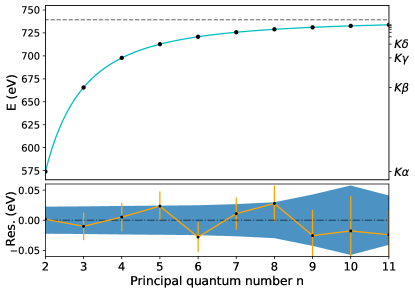
Figure 4: Fit of the Rydberg formula to the measured He-like $K$ series with nuclear effective charge Ze, quantum defect $\delta$ and ionization potential ($E_{\text{IP}}$) as a free parameter. The blue shaded area indicates the confidence interval.

Table 2: Fit results in comparison with available theoretical and experimental values.

	Fit	Scofield (2009)	Drake (1988)	Tupitsyn et al. (2020)
$E_{\text{IP}}$	739.336(16)	739.3	739.32682(6)	739.326262
$\text{Z}_{\text{eff}}$	7.008(3)
$\delta$	$-0.0014(9)$

Hereafter, we refer the radiative decay channel towards the ground state as direct decay (DD), to distinguish from sequential two-photon decays (TPD), such as $1s\,2s\,3p\rightarrow 1s\,2s^{2}\rightarrow 1s^{2}\,2p$. Direct decay is the time-inverse process of photoexcitation (PE), and the overall process of PE plus DD is equivalent to elastic fluorescence emission, as apparent for $K{\beta_{1}}$ and $K\gamma$ in the decay spectrum of Fig. 3a. Figure 5 shows the decay spectra for $K{\beta_{1}}$ and $K\gamma$, confirming these DD channels.

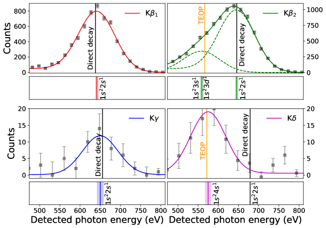
Figure 5: Fitted fluorescence decay spectra of the $K\beta_{1,2}$, $K\gamma$ and $K\delta$ absorption resonances in Li-like O⁵⁺ ions. Lines in the same color as the fit curves mark the corresponding decay energies (labeled by their respective final configuration), and the shaded area their uncertainties. The orange line shows the theoretical TEOP channel position and the black line the theoretical direct decay channel position. Here $K\beta_{1,2}$ contain data from separate scans with higher statistics and were fitted withthe addition of the Compton lower-energy tail.

However, as also displayed in Fig. 5, the 646-eV $K{\beta_{2}}$ line and $K\delta$ both reveal different radiative decay channels besides the expected DD. While $K{\beta_{2}}$ appears to have a minor contribution to the main elastic DD channel, $K{\delta}$ shows a dominant inelastic channel and no elastic one. To understand this, we performed calculations of the main decay channels of the lines presented in Fig. 5 with the Flexible Atomic Code (FAC) Gu (2008), which provide us with transition rates missing in the high-accuracy calculations of Yerokhin and Surzhykov (2019).

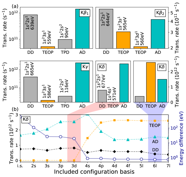
Figure 6: a) FAC transition-rate calculations for the strongest decay channels following resonant photoexcitation of the $K\beta_{1,2}$, $K{\gamma}$, and $K{\delta}$ transitions in O⁵⁺ ions, and b) their convergence depending on the configuration basis size (see the text). For $K{\delta}$, two stages of convergence are highlighted: red indicates incomplete and blue the final result. The respective final states and transition energies are labeled accordingly. Here DD denotes the direct one-photon decay to the ground state, TEOP the two-electron-one photon decay, TPD the two-photon decay cascade, and AD Auger decay.

While doubly-excited states commonly relax by AD, our FAC Gu (2008) calculations show that this channel is only relevant for $K{\beta_{1}}$ and $K{\gamma}$ (see Fig. 6), and also confirm a main DD for $K{\beta_{1}}$ and $K{\gamma}$. After PE of $K{\beta_{2}}$, DD competes with the TEOP transition feeding into the $1s^{2}\,3s$ and $1s^{2}\,3d$ states (roughly 5 eV apart) that can radiatively decay through various cascades. This results from configuration mixing with the $1s\,2p\,3s$ and $1s\,2p\,3d$ states. For $K\delta$, no significant DD could be observed. Here, the upper state dominantly relaxes through a TEOP transition to the $1s^{2}\,4s$ state.

The question is, what makes the usual DD to the ground state so weak? As shown in Fig. 3c, the excited $1s\,2s\,5p$ state has a near degeneracy ($0.8$ eV) with a state of the same total angular momentum and parity, $1s\,2p\,4s$, which is also the upper state of a Li-like satellite of the He-like $K\alpha$ line. Thus, the excited states strongly mix with these, which have much higher decay rates towards $1s^{2}\,4s$ (on the order of ${10}^{12}\text{\,}\mathrm{s}$^-1). This suppresses the one-photon DD to the ground state, as can be seen in Fig. 5.

Table 3: Configurations added to the CI basis set for each calculation having the CI label of Fig. 7; each set keeps all the configurations of the sets above it.

CI label	Configuration set
initial set	$1s^{2}2l$
	$1s^{2}4l$
	$1s2s5l$
$2l$	$1s2l2l^{\prime}$
$3s$	$1s^{2}3s$
	$1s2l3s$
$3p$	$1s^{2}3p$
	$1s2l3p$
$3d$	$1s^{2}3d$
	$1s2l3d$
$4s$	$1s2l4s$
$4p$	$1s2l4p$
$4d$	$1s2l4d$
$4f$	$1s2l4f$
$5l$	$1s^{2}5l$
$6l$	$1s^{2}6l$
	$1s2l6l^{\prime}$
$7l$	$1s^{2}7l$
	$1s2l7l^{\prime}$

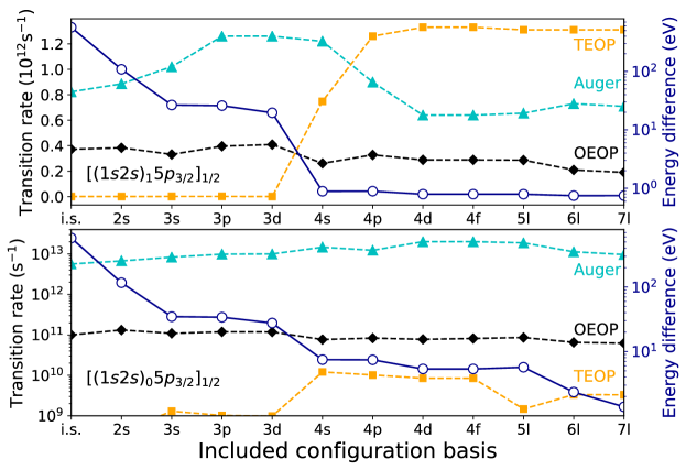
Figure 7: Calculated decay rates and energy degeneracies of the initial states $[(1s2s)_{1}5p_{3/2}]_{1/2}$ (top) and $[(1s2s)_{0}5p_{3/2}]_{1/2}$ (bottom) with different CI basis sets (see Table 3 in text). Both transition rates to final states $[1s^{2}2s]_{1/2}$ (the OEOP transition) and $[1s^{2}4s]_{1/2}$ (the TEOP transition) are included, along with the Auger rate to $1s^{2}$ state (left y-scale). Open circles represent the energy difference (degeneracy) in eV (right y-scale).

Table 4: Core-hole relaxation following $K\beta_{1,2}$, $K{\gamma}$, and $K{\delta}$ resonant photon excitation in O⁵⁺ ions. The first column lists the excitation transitions. Subsequent columns indicate the decay channels’ respective initial and final configurations, peak photon energies (from the silicon-drift detector), final-state energies (calculated with FAC Gu (2008)), and transition type (DD denotes direct photon decay, and TEOP the two-electron–one-photon transition). The DD-to-TEOP intensity ratio is also given. All energies are in eV.

Line	Initial configuration	Final configuration	Photon energy	FAC	Type
$K\beta_{1}$	$1s\,2s\,3p$	$1s^{2}\,2s$	641.68(3.3)	638.50	DD
$K\beta_{2}$	$1s\,2s\,3p$	$1s^{2}\,2s$	645.8(3.3)	644.70	DD
$K\beta_{2}$	$1s\,2s\,3p$	$1s^{2}\,3s$	559.4(3.8)	565.40	TEOP
		$1s^{2}\,3d$	blend	560.2	TEOP
$K\gamma$	$1s\,2s\,4p$	$1s^{2}\,2s$	650.2(7.8)	665.30	DD
$K\delta$	$1s\,2s\,5p$	$1s^{2}\,4s$	574.9(7.6)	570.71	TEOP
branching ratio	$K\beta_{2}$	DD-to-TEOP ratio	Exp.: 1.73(19)	FAC: 1.39

IV.2 Role of configuration mixing: Calculations

We investigate the underlying quantum processes by calculating electronic energies, transition rates, and Auger rates with the relativistic configuration-interaction package FAC Gu (2008). The convergence of the configuration mixing was studied by varying the size of the configuration-interaction (CI) basis set, as listed in Table 3. This allowed us to identify the key configurations leading to a strong TEOP rate.

Figure 7 displays the effect of the CI basis size on the transition rates from the upper state $[(1s2s)_{1}5p_{3/2}]_{1/2}$ towards the final states $[1s^{2}2s]_{1/2}$ (the OEOP transition) and $[1s^{2}4s]_{1/2}$ (the TEOP transition), and on the Auger rate to the $1s^{2}$ state (the only possible Auger channel). All the decay rates have an allowed electric dipole contribution that dominates higher-order multipoles. The energy degeneracy, defined as the smallest energy difference between this initial state and the nearest one having the same total momentum and parity symmetry in a different configuration, is also represented. While the OEOP rate is nearly independent of the CI-basis set, a sudden increase of three orders of magnitude in the TEOP transition appears when the $1s2p4s$ configuration is included, which leads to a mixed state with contributions of order of 75% from $[(1s2s)_{1}5p_{1/2,3/2}]_{1/2}$ and of order of 25% from $[(1s2p_{1/2,3/2})_{1}4s]_{1/2}$. Adding further configurations lets the TEOP rate converge towards a value that is approximately twice that of the Auger process, and eight times that of OEOP decay. The above-mentioned energy degeneracy becomes more pronounced with the inclusion of further configurations, as the energy separation decreases from tens of eV to order of 0.8 eV. This causes the mixing coefficient to grow by order of 28% for $[(1s2p_{1/2,3/2})_{1}4s]_{1/2}$, which combined with the high decay rate of the $[1s2p4s]_{1/2}\rightarrow[1s^{2}4s]_{1/2}$ transition (the satellite of the He-like $K\alpha$) makes the TEOP rate for $[1s2s5p]$ predominant. The initial $[(1s2s)_{1}5p_{3/2}]_{3/2}$ state also follows a similar behavior. The Auger rates drop due to mixing with configurations of higher orbital momentum having lower Auger rates. The TEOP rate for the initial state $[(1s2s)_{0}5p_{1/2}]_{1/2}$ does not show a significant increase with inclusion of $[1s2p4s]_{1/2}$ in the basis set. This is due to the energy difference with $[1s^{2}4s]_{1/2}$ being of order of a few eV, which reduces the mixing coefficient of the $[1s2p4s]_{1/2}$ configuration to 1.3%.

Summarizing our theoretical analysis, Fig. 6 shows that including the near degenerate $1s\,2p\,4s\,$ state in the calculation of the $K\delta$ decay rates increases the TEOP rate by more than three orders of magnitude. Besides this, we also checked another plausible photoexcitation channel $1s^{2}\,2s\,\rightarrow$ $1s\,2p\,4s\,$ that can also decay to $1s^{2}\,4s$ ground state. This alternative path can possibly further enhance the observed TEOP channel. However, a comparison of photoexcitation rates between $1s^{2}\,2s\,\rightarrow$ $1s\,2p\,4s\,$ (approximately equal to $2\times 10^{10}~{}\mbox{s}^{-1}$) and $1s^{2}\,2s\,\rightarrow$ $1s\,2s\,5p\,$ (approximately equal to $1\times 10^{11}~{}\mbox{s}^{-1}$) shows an order of magnitude difference between them. Therefore, we emphasize that the $1s\,2p\,4s\,$ state can only be populated via $K\delta$ photoexcitation and decay via the TEOP channel, as observed in the present experiment.

IV.3 Determination of the ratio DD/TEOP

Our measured $K{\beta_{2}}$ decay energies are listed in Table 4. Because the respective fluorescence-decay channels can be barely resolved by the SDD (cf. Fig. 5), their centroids were only determined with an uncertainty in the 0.5–1.3% range; this can be improved in the future, e. g., by using a high-resolution x-ray microcalorimeter Durkin et al. (2019). Since measuring line ratios is an essential plasma diagnostic tool, and stringently tests theory, we extract the ratio of the DD rate to the TEOP transition rate from the measured spectra (Fig. 5). While the DD-to-TEOP ratio of $K\delta$ could not be accurately determined due to low statistics in the DD channel, it was nonetheless possible to quantify the DD-to-TEOP ratio for the Li-like $K\beta_{2}$ emission. For this we characterized the x-ray detector taking into account the transmission of the 500-nm Al filter placed in front of it to block visible and UV radiation, and also the low-energy Compton tail of the detector response line shape. This tail was obtained from a fit to the $K\beta_{1}$ transition, which should only have the elastic channel, as configuration mixing with other states is small, and used as fit function for the DD channel of $K\beta_{2}$. We estimate the uncertainty of the Al-filter transmission from its thickness ($500\pm 100$ nm), adding a contribution of $\pm 15\%$ to the ratio-error budget. The soft x-ray spectral sensitivity of the SDD strongly depends on the thickness of native silicon dioxide layer on its surface, which is not well known (20 to 50 nm), on the top-electrode materials, and on the slow condensation of water on its cold surface during the experiment. Since one of the decay channels (the TEOP transition) of $K\beta_{2}$ is close to the oxygen $K$ edge, these layers can significantly change the ratio of the transmission coefficients for the $1s2s3p\rightarrow 1s^{2}$ transition at 644 eV versus the one of the $1s2s3p\rightarrow 1s^{2}3d$ at 565 eV. With these caveats, and assuming a filter transmission ratio (644 eV-to-565 eV) approximately equal to $1.25\pm 0.2$ and a SDD sensitivity ratio (644 eV-to-565 eV) of approximately $1.15\pm 0.5$, the observed intensity ratio of 2.93 yields a ratio of approximately $2.0\pm 0.8$, which is compatible with the FAC prediction.

Table 5: Decay rates for the $K\beta_{2}$ states $[(1s2s)_{0}3p_{1/2}]_{1/2}$ ($J=1/2$) and $[(1s2s)_{0}3p_{3/2}]_{3/2}$ ($J=3/2$). Values are in s^-1.

State	DD rate	TEOP rate
	$1s^{2}2s$	$1s^{2}3s$	$1s^{2}3d_{3/2}$	$1s^{2}3d_{5/2}$
$J=1/2$	$3.24\times 10^{11}$	$1.17\times 10^{11}$	$1.03\times 10^{11}$
$J=3/2$	$3.21\times 10^{11}$	$1.29\times 10^{11}$	$1.02\times 10^{10}$	$9.25\times 10^{10}$

In a second approach, we determine the DD-to-TEOP ratio by comparing the intensity ratio K$\alpha$/K$\beta=2.06\pm 0.05$ of the simultaneously observed He-like transitions with the ratio of their theoretical Einstein coefficients, $A_{ik}/A_{ik^{\prime}}=3.53$ according to the NIST database Kramida et al. . We normalize the observed intensities to the excitation-photon flux, and obtain a sensitivity ratio (665.61 eV-to-573.94 eV) approximately equal to $1.70\pm 0.17$, whereby the decay channels very closely match the energies of the Li-like transitions under investigation. This takes into account all previously mentioned effects of the filter and detector efficiency. When we interpolate this sensitivity ratio to the close-by Li-like transitions, the observed intensity ratio (approximately equal to 2.93) for the Li-like K$\beta_{2}$ decay channels results in a ratio of approximately 1.73$\pm$0.19, in fair agreement with our FAC calculation.

Emission of $K\beta_{2}$ follows PE of the states $[(1s2s)_{0}3p_{1/2}]_{1/2}$ and $[(1s2s)_{0}3p_{3/2}]_{3/2}$ feeding the radiative decay channels listed in Table 5. Their respective strengths yield a DD-to-TEOP ratio of 1.39 for an observation angle of $90^{\circ}$ (see the Appendix) and 1.43 for the solid-angle integrated total emission. Note that the decay rates from these states to the ground state are similar and likewise the corresponding PE cross sections. This cancels the effect of state population on the ratio.

Table 6: Angular coefficients $\beta_{J_{d}\rightarrow J_{f}}$ for angular momenta $J_{d}$ and $J_{f}$.

${J_{d}\rightarrow J_{f}}$ $\begin{array}[]{c}\\ \frac{1}{2}\rightarrow 1/2\end{array}$	$\frac{1}{2}\rightarrow\frac{1}{2}$	$\frac{1}{2}\rightarrow\frac{3}{2}$	$\frac{3}{2}\rightarrow\frac{1}{2}$	$\frac{3}{2}\rightarrow\frac{3}{2}$	$\frac{3}{2}\rightarrow\frac{5}{2}$
$\beta_{J_{d}\rightarrow J_{f}}$	0	0	$-\frac{1}{2}$	$\frac{2}{5}$	$-\frac{1}{10}$

V Conclusion

We have demonstrated how a complex process that is difficult to disentangle in astrophysical plasmas can be isolated and studied in detail by high-resolution photon excitation. Unexpectedly strong TEOP transitions were found in an essential species, the relatively simple Li-like O⁵⁺, showing, among other observations, evidence that the upper state of the $K\delta$ line in Li-like O⁵⁺ mainly decays as a satellite of He-like O⁶⁺ $K\alpha$. This produces a problematic blend in a key feature for the diagnostics of photoionized plasmas (e.g. Mehdipour et al. (2015)). Although a strong suppression of the direct photo decay by TEOP transitions was observed in just one of several lines in Li-like oxygen, it is not far-fetched to assume that TEOP-dominated relaxation also happens in other multiply excited, multi-electron systems, and thus its contribution should not be neglected in accurate astrophysical plasma models.

Systems with more than three electrons have richer overlapping excitations with manifold decay channels not only cause similar blends in emission and absorption spectra, but also affect the ionization balance of plasmas. The three-electron system studied here is more tractable by current theory and has allowed us to stringently test the underlying electronic correlations. This is of great importance for the diagnostics of hot gas in astrophysics. The upcoming launches of XRISM Tashiro et al. (2018) and Athena Barret et al. (2016) urgently call for studying the position and strength of TEOP transitions that can cause shifts, or broaden the strong diagnostically important O-$K$ and Fe-$L$ lines in the 15–23 Å range, which are crucial for determining gas-outflow velocities of warm absorbers and density diagnostics of photoionized plasmas Drake et al. (1999); Behar et al. (2003); Schmidt et al. (2004); Gu et al. (2005); Mehdipour et al. (2015), and needed for accurately modeling the x-ray continuum flux.

Appendix A ANGULAR DISTRIBUTION

In our experiment, fluorescence photons were observed at $90^{\circ}$, so we took into account the angular distribution pattern of their emission in the experimental determination of the DD-to-TEOP ratio. We treated PE and subsequent radiative decay as a two-step process within the $E1$ dipole approximation, which is appropriate as the main multipole channel of both the TEOP transition and DD transition is of $E1$ type. We assume that the ground state is not initially aligned, allowing us to apply for the angular distribution the formula given by Balashov et al. (2000),

$$W(\theta)=\frac{W_{0}}{4\pi}\left(1-\frac{\beta_{J_{d}\rightarrow J_{f}}}{2}P_{2}(\cos{\theta})\right).$$

This formula is valid for circularly polarized incident photons, as in the present experiment, and yields a dependence of the radial angle $\theta$ ($z$ axis or quantization axis alongside the incident photon beam propagation axis and magnetic field) in terms of a second rank Legendre polynomial $P_{2}$, with $W_{0}$ being the total emission. The angular coefficients $\beta_{J_{d}\rightarrow J_{f}}$ from the photoexcited state with total angular momentum $J_{d}$ to various final states of interest for the case $K\beta_{2}$ are given in Table 6.

References

- Beiersdorfer (2003) P. Beiersdorfer, Annual Review of Astronomy and Astrophysics 41, 343 (2003).
- Tashiro et al. (2018) M. Tashiro, H. Maejima, K. Toda, R. Kelley, L. Reichenthal, J. Lobell, R. Petre, M. Guainazzi, E. Costantini, M. Edison, et al., Proc. SPIE 10699, 1069922 (2018).
- Barret et al. (2016) D. Barret, T. L. Trong, J.-W. Den Herder, L. Piro, X. Barcons, J. Huovelin, R. Kelley, J. M. Mas-Hesse, K. Mitsuda, S. Paltani, et al., Space Telescopes and Instrumentation 2016: Ultraviolet to Gamma Ray 9905, 99052F (2016).
- Hell et al. (2020) N. Hell, P. Beiersdorfer, G. V. Brown, M. E. Eckart, R. L. Kelley, C. A. Kilbourne, M. A. Leutenegger, T. E. Lockard, F. S. Porter, and J. Wilms, X-Ray Spectrometry 49, 218 (2020).
- Simcoe et al. (2002) R. A. Simcoe, W. L. W. Sargent, and M. Rauch, Astrophys. J 578, 737 (2002).
- Nicastro et al. (2018) F. Nicastro, J. Kaastra, Y. Krongold, S. Borgani, E. Branchini, R. Cen, M. Dadina, C. W. Danforth, M. Elvis, F. Fiore, et al., Nature 558, 406 (2018).
- Gatuzz et al. (2019) E. Gatuzz, J. A. García, and T. R. Kallman, Mon. Not. R. Astron. Soc. 483, L75 (2019).
- Kallman and Palmeri (2007) T. R. Kallman and P. Palmeri, Rev. Mod. Phys. 79, 79 (2007).
- Gorczyca (2004) T. Gorczyca, Radiat. Phys. Chem. 70, 407 (2004).
- Schippers et al. (2016a) S. Schippers, R. Beerwerth, L. Abrok, S. Bari, T. Buhr, M. Martins, S. Ricz, J. Viefhaus, S. Fritzsche, and A. Müller, Phys. Rev. A 94, 041401(R) (2016a).
- Müller et al. (2018) A. Müller, A. Borovik, S. Bari, T. Buhr, K. Holste, M. Martins, A. Perry-Saßmannshausen, R. A. Phaneuf, S. Reinwardt, S. Ricz, et al., Phys. Rev. Lett. 120, 133202 (2018).
- Perry-Sassmannshausen et al. (2020) A. Perry-Sassmannshausen, T. Buhr, A. Borovik, M. Martins, S. Reinwardt, S. Ricz, S. O. Stock, F. Trinter, A. Müller, S. Fritzsche, and S. Schippers, Phys. Rev. Lett. 124, 083203 (2020).
- West (2001) J. B. West, J. Phys. B: At., Mol. Opt. Phys. 34, R45 (2001).
- Kjeldsen (2006) H. Kjeldsen, J. Phys. B: At., Mol. Opt. Phys. 39, R325 (2006).
- Bizau et al. (2015) J. M. Bizau, D. Cubaynes, S. Guilbaud, M. M. Al Shorman, M. F. Gharaibeh, I. Q. Ababneh, C. Blancard, and B. M. McLaughlin, Phys. Rev. A 92, 023401 (2015).
- Berrah et al. (2004) N. Berrah, J. Bozek, R. Bilodeau, and E. Kukk, Radiat. Phys. Chem. 70, 57 (2004), photoeffect: Theory and Experiment.
- Gharaibeh et al. (2011) M. F. Gharaibeh, A. Aguilar, A. M. Covington, E. D. Emmons, S. W. J. Scully, R. A. Phaneuf, A. Müller, J. D. Bozek, A. L. D. Kilcoyne, A. S. Schlachter, et al., Phys. Rev. A 83, 043412 (2011).
- Levin and Armen (2004) J. C. Levin and G. Armen, Radiat. Phys. Chem. 70, 105 (2004), photoeffect: Theory and Experiment.
- Kabachnik et al. (2007) N. Kabachnik, S. Fritzsche, A. Grum-Grzhimailo, M. Meyer, and K. Ueda, Phys. Rep. 451, 155 (2007).
- Southworth et al. (2019) S. H. Southworth, R. W. Dunford, D. Ray, E. P. Kanter, G. Doumy, A. M. March, P. J. Ho, B. Krässig, Y. Gao, C. S. Lehmann, et al., Phys. Rev. A 100, 022507 (2019).
- Ma et al. (2017) Y. Ma, F. Zhou, L. Liu, and Y. Qu, Phys. Rev. A 96, 042504 (2017).
- Dunford et al. (2004) R. Dunford, E. Kanter, B. Krässig, S. Southworth, and L. Young, Radiat. Phys. Chem. 70, 149 (2004), photoeffect: Theory and Experiment.
- Schippers et al. (2016b) S. Schippers, A. L. D. Kilcoyne, R. A. Phaneuf, and A. Müller, Contemp. Phys. 57, 215 (2016b).
- Müller et al. (2017) A. Müller, D. Bernhardt, A. Borovik, T. Buhr, J. Hellhund, K. Holste, A. L. D. Kilcoyne, S. Klumpp, M. Martins, S. Ricz, et al., Astrophys. J 836, 166 (2017).
- Blancard et al. (2018) C. Blancard, D. Cubaynes, S. Guilbaud, and J.-M. Bizau, Astrophys. J 853, 32 (2018).
- Simon et al. (2010) M. C. Simon, J. R. Crespo López-Urrutia, C. Beilmann, M. Schwarz, Z. Harman, S. W. Epp, B. L. Schmitt, T. M. Baumann, E. Behar, S. Bernitt, et al., Phys. Rev. Lett. 105, 183001 (2010).
- Steinbrügge et al. (2015) R. Steinbrügge, S. Bernitt, S. W. Epp, J. K. Rudolph, C. Beilmann, H. Bekker, S. Eberle, A. Müller, O. O. Versolato, H.-C. Wille, et al., Phys. Rev. A 91, 032502 (2015).
- Bliman et al. (1989) S. Bliman, P. Indelicato, D. Hitz, P. Marseille, and J. P. Desclaux, Journal of Physics B: Atomic, Molecular and Optical Physics 22, 2741 (1989).
- Tawara and Richard (2002) H. Tawara and P. Richard, Canadian Journal of Physics, Canadian Journal of Physics 80, 1579 (2002).
- Kato et al. (2006) D. Kato, N. Nakamura, and S. Ohtani, J. Plasma Fusion Res. SERIES 7, 190 (2006).
- Young et al. (2010) L. Young, E. P. Kanter, B. Krässig, Y. Li, A. M. March, S. T. Pratt, R. Santra, S. H. Southworth, N. Rohringer, L. F. DiMauro, et al., Nature 466, 56 (2010).
- Buth et al. (2018) C. Buth, R. Beerwerth, R. Obaid, N. Berrah, L. S. Cederbaum, and S. Fritzsche, J. Phys. B: At., Mol. Opt. Phys. 51, 055602 (2018).
- Beiersdorfer et al. (1992) P. Beiersdorfer, T. W. Phillips, K. L. Wong, R. E. Marrs, and D. A. Vogel, Phys. Rev. A 46, 3812 (1992).
- Nakamura et al. (2008) N. Nakamura, A. P. Kavanagh, H. Watanabe, H. A. Sakaue, Y. Li, D. Kato, F. J. Currell, and S. Ohtani, Phys. Rev. Lett. 100, 73203 (2008).
- Shah et al. (2015) C. Shah, H. Jörg, S. Bernitt, S. Dobrodey, R. Steinbrügge, C. Beilmann, P. Amaro, Z. Hu, S. Weber, S. Fritzsche, et al., Phys. Rev. A 92, 042702 (2015).
- Schnell et al. (2003) M. Schnell, G. Gwinner, N. R. Badnell, M. E. Bannister, S. Böhm, J. Colgan, S. Kieslich, S. D. Loch, D. Mitnik, A. Müller, et al., Phys. Rev. Lett. 91, 043001 (2003).
- Beilmann et al. (2011) C. Beilmann, P. H. Mokler, S. Bernitt, C. H. Keitel, J. Ullrich, J. R. Crespo López-Urrutia, and Z. Harman, Phys. Rev. Lett. 107, 143201 (2011).
- Shah et al. (2016) C. Shah, P. Amaro, R. Steinbrügge, C. Beilmann, S. Bernitt, S. Fritzsche, A. Surzhykov, J. R. Crespo López-Urrutia, and S. Tashenov, Phys. Rev. E 93, 061201(R) (2016).
- Drake et al. (1999) J. J. Drake, D. A. Swartz, P. Beiersdorfer, G. V. Brown, and S. M. Kahn, Astrophys. J 521, 839 (1999).
- Liu et al. (2018) P. Liu, J. Zeng, and J. Yuan, J. Phys. B: At., Mol. Opt. Phys. 51, 075202 (2018).
- Zaytsev et al. (2019) V. A. Zaytsev, I. A. Maltsev, I. I. Tupitsyn, and V. M. Shabaev, Phys. Rev. A 100, 052504 (2019).
- Behar et al. (2001) E. Behar, M. Sako, and S. M. Kahn, Astrophys. J 563, 497 (2001).
- McLaughlin et al. (2016) B. M. McLaughlin, J.-M. Bizau, D. Cubaynes, S. Guilbaud, S. Douix, M. M. A. Shorman, M. O. A. E. Ghazaly, I. Sakho, and M. F. Gharaibeh, Mon. Not. R. Astron. Soc. 465, 4690 (2016).
- Mathur et al. (2017) S. Mathur, F. Nicastro, A. Gupta, Y. Krongold, B. M. McLaughlin, N. Brickhouse, and A. Pradhan, Astrophys. J 851, L7 (2017).
- Viefhaus et al. (2013) J. Viefhaus, F. Scholz, S. Deinert, L. Glaser, M. Ilchen, J. Seltmann, P. Walter, and F. Siewert, Nucl. Instrum. Methods Phys. Res 710, 151 (2013), the 4th international workshop on Metrology for X-ray Optics, Mirror Design, and Fabrication.
- Micke et al. (2018) P. Micke, S. Kühn, L. Buchauer, J. R. Harries, T. M. Bücking, K. Blaum, A. Cieluch, A. Egl, D. Hollain, S. Kraemer, et al., Rev. Sci. Instrum. 89, 063109 (2018).
- Kühn et al. (2020) S. Kühn, C. Shah, J. R. Crespo López-Urrutia, K. Fujii, R. Steinbrügge, J. Stierhof, M. Togawa, Z. Harman, N. S. Oreshkina, C. Cheung, et al., Phys. Rev. Lett. 124, 225001 (2020).
- Yerokhin and Surzhykov (2019) V. A. Yerokhin and A. Surzhykov, J. Phys. Chem. Ref. Data 48, 033104 (2019).
- Drake (1988) G. W. Drake, Can. J. Phys. 66, 586 (1988).
- Tupitsyn et al. (2020) I. I. Tupitsyn, S. V. Bezborodov, A. V. Malyshev, D. V. Mironova, and V. M. Shabaev, Optics and Spectroscopy 128, 21 (2020).
- Yerokhin et al. (2017) V. A. Yerokhin, A. Surzhykov, and A. Müller, Phys. Rev. A 96, 069901 (2017).
- Savukov et al. (2003) I. Savukov, W. Johnson, and U. Safronova, Atomic Data and Nuclear Data Tables 85, 83 (2003).
- Natarajan (2015) L. Natarajan, Phys. Rev. A 92, 012507 (2015).
- (54) A. Kramida, Yu. Ralchenko, J. Reader, and and NIST ASD Team, NIST Atomic Spectra Database (ver. 5.7.1), [Online]. Available: https://physics.nist.gov/asd [2017, April 9]. National Institute of Standards and Technology, Gaithersburg, MD.
- Engstrom and Litzen (1995) L. Engstrom and U. Litzen, Journal of Physics B: Atomic, Molecular and Optical Physics 28, 2565 (1995).
- Scofield (2009) J. Scofield, “X-ray data booklet,” (2009).
- Heisenberg (1925) W. Heisenberg, Zeitschrift für Physik 32, 841 (1925).
- Condon (1930) E. U. Condon, Phys. Rev. 36, 1121 (1930).
- Goudsmit and Gropper (1931) S. Goudsmit and L. Gropper, Phys. Rev. 38, 225 (1931).
- Wölfli et al. (1975) W. Wölfli, C. Stoller, G. Bonani, M. Suter, and M. Stöckli, Phys. Rev. Lett. 35, 656 (1975).
- Briand et al. (1974) J. P. Briand, P. Chevallier, A. Johnson, J. P. Rozet, M. Tavernier, and A. Touati, Phys. Lett. A 49, 51 (1974).
- Mikkola et al. (1979) E. Mikkola, O. Keski-Rahkonen, and R. Kuoppala, Phys. Scr. 19, 29 (1979).
- Stoller et al. (1977) C. Stoller, W. Wölfli, G. Bonani, M. Stöckli, and M. Suter, Phys. Rev. A 15, 990 (1977).
- Ahopelto et al. (1979) J. Ahopelto, E. Rantavuori, and O. Keski-Rahkonen, Phys. Scr. 20, 71 (1979).
- Salem et al. (1982) S. I. Salem, A. Kumar, B. L. Scott, and R. D. Ayers, Phys. Rev. Lett. 49, 1240 (1982).
- Salem et al. (1984) S. I. Salem, A. Kumar, and B. L. Scott, Phys. Rev. A 29, 2634 (1984).
- Auerhammer et al. (1988) J. Auerhammer, H. Genz, A. Kumar, and A. Richter, Phys. Rev. A 38, 688 (1988).
- Rosmej et al. (2001) F. B. Rosmej, D. H. H. Hoffmann, W. Süß, M. Geißel, A. Y. Faenov, and T. A. Pikuz, Phys. Rev. A 63, 032716 (2001).
- Zou et al. (2003) Y. Zou, J. R. Crespo López-Urrutia, and J. Ullrich, Phys. Rev. A 67, 042703 (2003).
- Harman et al. (2019) Z. Harman, C. Shah, A. J. González Martínez, U. D. Jentschura, H. Tawara, C. H. Keitel, J. Ullrich, and J. R. Crespo López-Urrutia, Phys. Rev. A 99, 012506 (2019).
- Kelly (1976) H. P. Kelly, Phys. Rev. Lett. 37, 386 (1976).
- Åberg et al. (1976) T. Åberg, K. A. Jamison, and P. Richard, Phys. Rev. Lett. 37, 63 (1976).
- Gavrila and Hansen (1978) M. Gavrila and J. E. Hansen, J. Phys. B: At. Mol. Phys. 11, 1353 (1978).
- Baptista (1986) G. B. Baptista, J Phys B: At Mol Phys 19, 159 (1986).
- Mukherjee and Ghosh (1988) T. K. Mukherjee and K. K. Ghosh, Phys. Rev. A 37, 4985 (1988).
- Saha et al. (2009) J. K. Saha, T. K. Mukherjee, S. Fritzsche, and P. K. Mukherjee, Phys. Lett. A 373, 252 (2009).
- Kadrekar and Natarajan (2010) R. Kadrekar and L. Natarajan, J. Phys. B: At., Mol. Opt. Phys. 43, 155001 (2010).
- Natarajan and Kadrekar (2013) L. Natarajan and R. Kadrekar, Phys. Rev. A 88, 012501 (2013).
- Lyashchenko et al. (2020) K. N. Lyashchenko, O. Y. Andreev, and D. Yu, Phys. Rev. A 101, 040501 (2020).
- Indelicato (1997) P. Indelicato, Hyperfine Interact. 108, 39 (1997).
- Trotsenko et al. (2007) S. Trotsenko, T. Stöhlker, D. Banas, C. Z. Dong, S. Fritzsche, A. Gumberidze, S. Hagmann, S. Hess, P. Indelicato, Kozhuharov, et al., J. Phys. Conf. Ser. 58, 141 (2007).
- Marques et al. (2012) J. P. Marques, F. Parente, A. M. Costa, M. C. Martins, P. Indelicato, and J. P. Santos, Phys. Rev. A 86, 052521 (2012).
- Gu (2008) M. F. Gu, Can. J. Phys. 86, 675 (2008).
- Durkin et al. (2019) M. Durkin, J. S. Adams, S. R. Bandler, J. A. Chervenak, S. Chaudhuri, C. S. Dawson, E. V. Denison, W. B. Doriese, S. M. Duff, F. M. Finkbeiner, et al., IEEE Transactions on Applied Superconductivity 29, 2904472 (2019).
- Mehdipour et al. (2015) M. Mehdipour, J. S. Kaastra, and A. J. J. Raassen, Astron. Astrophys 579, A87 (2015).
- Behar et al. (2003) E. Behar, A. P. Rasmussen, A. J. Blustin, M. Sako, S. M. Kahn, J. S. Kaastra, G. Branduardi-Raymont, and K. C. Steenbrugge, Astrophys. J 598, 232 (2003).
- Schmidt et al. (2004) M. Schmidt, P. Beiersdorfer, H. Chen, D. B. Thorn, E. Träbert, and E. Behar, Astrophys. J 604, 562 (2004).
- Gu et al. (2005) M. F. Gu, M. Schmidt, P. Beiersdorfer, H. Chen, D. B. Thorn, E. Träbert, E. Behar, and S. M. Kahn, Astrophys. J 627, 1066–1071 (2005).
- Balashov et al. (2000) V. V. Balashov, A. N. Grum-Grzhimailo, and N. M. Kabachnik, Polarization and Correlation Phenomena in Atomic Collisions - A Practical Theory Course (Kluwer Academics/Plenum Publishers, 2000).