Constraining the Source of the High-velocity Ejecta in Type Ia SN 2019ein

Abstract

We present multiwavelength photometric and spectroscopic observations of SN 2019ein, a high-velocity Type Ia supernova (SN Ia) discovered in the nearby galaxy NGC 5353 with a two-day nondetection limit. SN 2019ein exhibited some of the highest measured expansion velocities of any SN Ia, with a Si II absorption minimum blueshifted by 24,000 km s^-1 at 14 days before peak brightness. More unusually, we observed the emission components of the P Cygni profiles to be blueshifted upward of 10,000 km s^-1 before B-band maximum light. This blueshift, among the highest in a sample of 28 other Type Ia supernovae, is greatest at our earliest spectroscopic epoch and subsequently decreases toward maximum light. We discuss possible progenitor systems and explosion mechanisms that could explain these extreme absorption and emission velocities. Radio observations beginning 14 days before B-band maximum light yield nondetections at the position of SN 2019ein, which rules out symbiotic progenitor systems, most models of fast optically thick accretion winds, and optically thin shells of mass $\lesssim 10^{-6}$ M_⊙ at radii $<100$ AU. Comparing our spectra to models and observations of other high-velocity SNe Ia, we find that SN 2019ein is well fit by a delayed-detonation explosion. We propose that the high emission velocities may be the result of abundance enhancements due to ejecta mixing in an asymmetric explosion, or optical depth effects in the photosphere of the ejecta at early times. These findings may provide evidence for common explosion mechanisms and ejecta geometries among high-velocity SNe Ia.

2020 July 10

1 Introduction

Supernovae Ia (SNe Ia) are thermonuclear explosions involving at least one white dwarf (WD) progenitor star (Bloom et al., 2012). A unique characteristic of SNe Ia is that they show a relationship between their peak luminosity and the width of their light curve, known as the Phillips relation (Phillips, 1993). This correlation allows the calibration of absolute brightness by light curve shape, which enables the determination of distances on cosmological scales. As standardizable candles, observations of SNe Ia have revealed the existence of dark energy (e.g. Riess et al. 1998; Schmidt et al. 1998; Perlmutter et al. 1999) and allow for a low-redshift measurement of the Hubble constant (e.g. Riess et al. 2019). A better understanding of their progenitor systems, explosion mechanisms, and observational characteristics is important to mitigate systematic uncertainties in order to use these objects for cosmological measurements.

Over the last several decades, sky surveys and deep imaging have led to the discovery of thousands of SNe Ia (e.g. Guy et al. 2010; Silverman et al. 2012; Macaulay et al. 2019). Large samples have shown that significant diversity exists within the population of SNe Ia (e.g. Parrent, Friesen, & Parthasarathy 2014). Obtaining detailed observations of SNe Ia is important for understanding the sources of this diversity. While the majority of SNe Ia are “normal” and obey the Phillips relation, a sizeable minority of peculiar objects tends to show varied photometric and spectral evolution around peak brightness (e.g. Filippenko et al., 1992a, b; Phillips et al., 1992), suggesting that fundamental differences beyond luminosity exist in the population of SNe Ia.

Models of progenitor systems and explosion mechanisms have attempted to explain the observed photometric and spectroscopic heterogeneity. Most SN Ia progenitor systems are modeled by accretion onto a degenerate WD from a nondegenerate companion (the single-degenerate scenario, e.g. Whelan & Iben 1973) or by the accretion or merger of two degenerate WDs (the double-degenerate scenario, e.g. Iben & Tutukov 1984). In addition, a variety of theoretical explosion models have been able to reproduce observed characteristics of SNe Ia. One such model is a delayed-detonation explosion, where a (subsonic) deflagration flame transitions to a (supersonic) detonation at some transition density (Iwamoto et al., 1999; Nomoto et al., 2013). Delayed-detonation simulations are able to reproduce a wide variety of light-curve widths, ⁵⁶Ni masses, ejecta compositions, and ejecta velocities in Chandrasekhar-mass progenitor WDs (Khokhlov, 1991; Seitenzahl et al., 2013). Another popular model is the double-detonation explosion, in which a detonation of helium accreted onto the surface of a WD leads to a second detonation at the core of the star (Fink et al., 2010; Kromer et al., 2010; Woosley & Kasen, 2011).

Several observational classification schemes have been proposed that may indirectly probe these different physical models. Branch et al. (2006) propose one such scheme, in which SNe Ia are classified by the strength of their Si II absorption features at maximum light. Additionally, Wang et al. (2009) sort SNe Ia by their Si II velocities, measured from the minimum of the absorption trough at B-band maximum light, into two classes: a high-velocity (HV) class, with $v_{\text{SiII}}\gtrsim$ 12,000 km s^-1, and a normal class, with $v_{\text{SiII}}\lesssim$ 12,000 km s^-1. After maximum light, SNe Ia can be classified as either high-velocity gradient (HVG) or low-velocity gradient (LVG) if the measured Si II velocity gradient is above or below 70 km s^-1 day^-1, respectively (Benetti et al., 2005).

This diversity in velocity may arise from different distributions of Si in the outer layers of the ejecta, which in turn depend on the explosion mechanism. For instance, Mazzali et al. (2005) studied the Si II and Ca II absorption features in the Type Ia SN 1999ee and found that two separate components, separated by over 7,000 km s^-1, were visible in the spectra before B-band maximum light. The authors described these as high-velocity features (HVFs) and photospheric velocity features (PVFs) and suggested they could be the result of additional mass at HVs. Other studies have attributed HVFs, particularly of the Ca II NIR feature, to interactions between the SN shock wave and a shell of circumstellar material formed from the SN progenitor system (e.g. Gerardy et al. 2004; Mulligan, & Wheeler 2018; Mulligan & Wheeler 2017).

One distinguishing feature between explosion mechanisms is the symmetry of the ejecta. Kasen & Plewa (2007) modeled spectroscopically normal SNe Ia and found that in asymmetric explosions, the color evolution and Si II 6355 Å velocity evolution exhibit significant viewing-angle dependence. Additionally, Maund et al. (2010) found an empirical relation between the Si II 6355 Å velocity gradient, as originally defined by Benetti et al. (2005), and the polarization across the same line, which traces the degree of the Si asymmetry in the ejecta (see, e.g., Wang & Wheeler 2008 for a review). Therefore, a better understanding of the spectroscopic differences of SNe Ia is crucial to constraining their explosion mechanisms and ejecta geometries.

In this paper we present observations of SN 2019ein, an extreme HV SN Ia. Our early-time observations, beginning two weeks before maximum light, make SN 2019ein one of the best-studied HV SN Ia. The earliest spectral data at 14 days before B-band maximum light reveal some of the highest ejecta velocities ever measured. Perhaps more interestingly, the emission features in the P Cygni profile of SN 2019ein are blueshifted with respect to the redshift of its host galaxy. This systematic offset is greatest at very early times (several days after explosion) and gradually decreases as the SN evolves. Such a large emission shift sets SN 2019ein apart from other SNe Ia and hints at a puzzling explosion mechanism and ejecta geometry.

In Section 2, we detail our data acquisition, reduction, and analysis procedure. In Section 3, we present comprehensive early-time light curves from the near-ultraviolet (NUV) to the near-infrared (NIR), along with model fits and fitted parameters. In Section 4, we present spectra, measure velocities of absorption features, and compare observations with a delayed-detonation explosion model. In Section 5, we place limits on the nature of the progenitor system and the source of HV ejecta using early-time radio observations. In Section 6 we offer several possible explanations for the HV ejecta and blueshifted emission features exhibited by SN 2019ein. Finally, we conclude in Section 7.

2 Observations

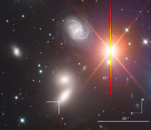
Figure 1: An RGB-color image of SN 2019ein (shown in the white crosshairs) in NGC 5353 along with its surrounding environment. A scale bar is shown in the bottom right corner. The image was produced using LCO 1m data files courtesy of Peter Iláš.

SN 2019ein was discovered on MJD 58604.47 (2019 May 1.47) by the ATLAS survey at magnitude 18.194 in their cyan filter (Tonry et al., 2019). The last nondetection of the transient was by the Zwicky Transient Facility (Bellm et al., 2019) in r band at a limit of 19.72 mag on MJD 58602.27 (2019 April 29.27), implying that SN 2019ein was discovered within two days after explosion. SN 2019ein exploded in the outskirts of NGC 5353, a lenticular galaxy in a nearby galaxy group. An image of NGC 5353 along with SN 2019ein is shown in Figure 1. Using surface brightness fluctuation measurements, J. Jensen et al. (2020, in preparation) measure the distance to NGC 5353 to be 32.96 $\pm$ 1.68 Mpc, and the redshift taken from the NASA/IPAC Extragalactic Database is 0.00775.

We began daily photometric and spectroscopic follow-up observations of SN 2019ein starting on 2019 May 2 with the Global Supernova Project using Las Cumbres Observatory (LCO; Brown et al. 2013). Our first spectrum, obtained with the FLOYDS spectrograph on the 2m telescope at Haleakal$\bar{\text{a}}$, allowed LCO to classify SN 2019ein as a young SN Ia (Burke et al., 2019). UBgVri-band data were obtained with the SBIG, Sinistro, and Spectral cameras on 0.4m, 1m, and 2m telescopes, respectively. With the PyRAF-based photometric reduction pipeline lcogtsnpipe (Valenti et al., 2016), PSF fitting was performed (Stetson, 1987). UBV-band photometry was calibrated to Vega magnitudes using Landolt standard fields (Landolt, 1992), while gri-band photometry were calibrated to AB magnitudes using the Sloan Digital Sky Survey (SDSS; SDSS Collaboration et al. 2017). Additionally, magnitudes were corrected for color terms using these standards. Because the SN was offset from the host galaxy, image subtraction was not necessary.

We obtained four epochs of NIR photometry in JHK_s filters with the 2MASS camera on the Minnesota-60$\arcsec$ telescope on Mt. Lemmon, AZ, as part of the Arizona Transient Exploration and Characterization (AZTEC) program. The data were reduced and stacked with the IRAF -xdimsum package. Aperture photometry was obtained with IRAF and calibrated to 20 local standards from the 2MASS catalog (Skrutskie et al., 2006).

We requested observations from the Ultraviolet and Optical Telescope (UVOT) on the Neil Gehrels Swift Observatory (Gehrels et al., 2004) after the detection of SN 2019ein. The first epoch of Swift data was obtained on MJD 58605.404 (2019 May 2.4), coincident with the first LCO photometric and spectroscopic epochs. Data were obtained in uvw2, uvm2, uvw1, u, b, and v filters and reduced using the data-reduction pipeline for the Swift Optical/Ultraviolet Supernova Archive (SOUSA; Brown et al. 2014), including applying aperture corrections and zero-points from Breeveld et al. (2011). Galaxy subtraction was not performed.

Table 1: Log of Spectroscopic Observations of SN 2019ein

MJD	Phasea	Wavelength Range [Å]	Telescope	Instrument
58605.3	-14	3200 – 10000	LCO 2m	FLOYDS
58609.5	-10	3500 – 10000	LCO 2m	FLOYDS
58613.4	-6	3500 – 10000	LCO 2m	FLOYDS
58615.3	-4	3500 – 10000	LCO 2m	FLOYDS
58618.2	-1	3500 – 10000	LCO 2m	FLOYDS
58619.2	0	3500 – 10000	LCO 2m	FLOYDS
58628.2	+9	3700 – 8000	Bok	BCSpec
58628.4	+9	3500 – 10000	LCO 2m	FLOYDS
58629.2	+10	3700 – 8000	Bok	BCSpec
58632.4	+13	3500 – 10000	LCO 2m	FLOYDS
58635.4	+16	3500 – 10000	LCO 2m	FLOYDS
58638.3	+19	5693 – 7000	MMT	Blue Channel
58640.3	+21	3700 – 8000	Bok	BCSpec
58641.4	+22	3500 – 10000	LCO 2m	FLOYDS
58647.3	+28	3500 – 10000	LCO 2m	FLOYDS
58651.3	+32	6875 – 25412	IRTF	SPeX
58653.4	+34	3500 – 10000	LCO 2m	FLOYDS
58666.4	+47	3500 – 10000	LCO 2m	FLOYDS
58679.3	+60	3500 – 10000	LCO 2m	FLOYDS

Note. — a: Days relative to B-band maximum light

Spectroscopic observations are detailed in Table 1. 14 LCO spectra were obtained using the FLOYDS instruments on LCO 2m telescopes at Siding Springs and Haleakal$\bar{\text{a}}$ between -14 days to 60 days with respect to B-band maximum. Our spectra cover approximately the entire optical range from 3500 to 10000 Å at resolution R $\approx$ 300-600. Data were reduced using the floydsspec custom pipeline, which performs flux and wavelength calibration, cosmic-ray removal, and spectrum extraction. In addition, we obtained several spectra in the optical and NIR using the B&C Spectrograph on the Bok 90$\arcsec$ telescope, the Blue Channel Spectrograph on the MMT at the Fred Lawrence Whipple Observatory, and the SpeX spectrograph (Rayner et al., 2003) in PRISM mode with a 0.5 $\times$ 15” slit on the NASA Infrared Telescope Facility, which was obtained and reduced following the methods in Hsiao et al. (2019). These data are presented in Section 4.

2.1 Radio Observations

Radio observations of SN 2019ein were obtained with the Karl G. Jansky Very Large Array (VLA) on 2019 May 3 within two days of discovery. Two follow-up observations about a week apart were subsequently obtained. Each observation was 1 hr long, with 37.6 minutes time on source per block for SN 2019ein. All observations were taken in C band (4-8 GHz) in the B configuration (program: 19A-010, PI: L. Chomiuk). The observations were obtained in wide-band continuum mode, yielding 4 GHz of bandwidth sampled by 32 spectral windows, each 64 MHz wide sampled by 2 MHz wide channels. We used 3C286 as our flux and bandpass calibrator, and J1419+3821 as our phase calibrator. Table 2 contains details of the observations.

Table 2: Summary of VLA Observations.

Epoch	Days Since	Synthesized Beam	3$\sigma$-upper Limitc
(MJDa)	Explosionb	(arcsec$\times$arcsec)	($\mu$Jy/beam)
58606.60	3.87	1.28$\times$1.27	17.88
58614.29	11.57	2.20$\times$1.23	25.32
58620.31	17.58	1.77$\times$1.99	23.46

Note. —

a: MJD at end of observation of each scheduling block

b: Assuming the explosion happened at most two days before discovery (Section 2). The explosion date corresponds to -16.93 days in units of phase relative to B-band maximum.

c: Three times the RMS noise at the site of SN 2019ein, inside a region of 6^′′ radius

We obtained the data sets processed by the VLA CASA calibration pipeline, run on CASA version 5.4.1. The pipeline consists of a collection of algorithms that automatically loads the raw data into a CASA measurement set (MS) format, flags corrupted data (e.g. due to antenna shadowing, channel edges, and radio frequency interference or RFI), applies various corrections (e.g. antenna position and atmospheric opacity) and derives delay, flux-scale, bandpass, and phase calibrations that are applied to the data.

For each epoch, the C-band data were split into 4-6 GHz and 6-8 GHz data sets, and each one was imaged using the CASA routine tclean. We use Briggs weighting of the data with a robust=0.7 to provide reasonable balance of angular resolution and source sensitivity. We used multiterm, multifrequency synthesis as our deconvolution algorithm (set with deconvolver=‘mtmfs’ in tclean), which performs deconvolution on a Taylor-series expansion of the wide-band spectral data in order to minimize frequency-dependent artifacts (Rau & Cornwell, 2011). We set nterms=2 which uses the first two Taylor terms to create images of intensity and spectral index. Multiple bright radio sources appear off-center in the 8.4^′ field of view, so we use “w-projection” (applied with gridder=‘wproject’ in tclean) to account for non-coplanar effects when deconvolving these sources (Cornwell et al., 2008). The radio nucleus of the host galaxy is the brightest radio source in the field (peak flux $\sim$ 25 mJy) and forms artifacts near the site of the SN, so we performed a phase-only self-calibration with a solution interval of 2 minutes to further clean and reduce the RMS noise in the image. The cleaned and self-calibrated 6-8 GHz image was then convolved to the resolution of the 4-6 GHz image using CONVL in AIPS. Both images were then combined using COMB in AIPS, weighted by their respective RMS noise, to create the final C-band image (central frequency of 6 GHz) of the SN 2019ein field.

No radio source was detected at the site of SN 2019ein in any of the cleaned deconvolved images down to 3$\sigma$ limits of $\sim$ 18 $\mu$Jy in the first image, and 25 and 23 $\mu$Jy in the subsequent images. We discuss the constraints on progenitor models set by these limits in Section 5.

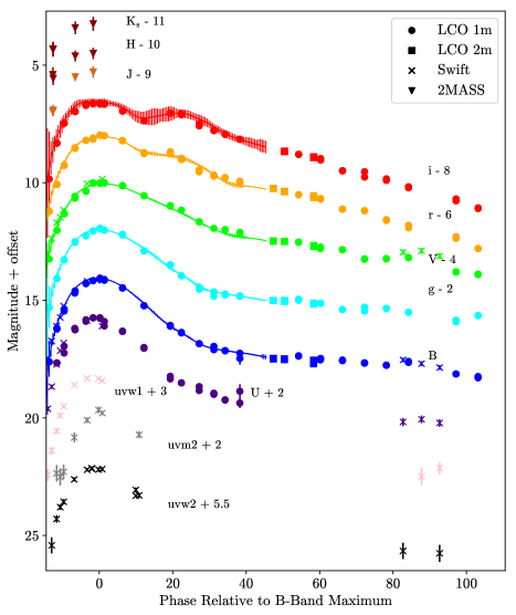
Figure 2: The NUV, optical, and NIR light curves of SN 2019ein, along with SALT2 fits and error bars to LCO data in BgVri filters (solid lines). The LCO UBgVri photometry is available as Data behind the Figure.

3 Photometric Results

3.1 Light Curves of SN 2019ein

Swift uvw2, uvm2, uvw1, Johnson-Cousins UBV, SDSS gri, and 2MASS JHK_s light curves are shown in Figure 2, along with SALT2 (Guy et al., 2007) fits to BgVri data between -14 days and 40 days with respect to B-band maximum light. Our high-cadence observations make the rise of this light curve extremely well-sampled. Because SN 2019ein was discovered quite early, we are able to tightly constrain the rise time and explosion time. Given the SALT2 fits to the light curve, we find the B-band maximum occurred at MJD 58619.45 $\pm$ 0.03 (2019 May 16.5), which implies a rise time of $\approx 14$ days since the beginning of observations and a maximum of $17$ days since explosion (all phases hereafter are given in terms of B-band maximum light). Using an expanding fireball model, Kawabata et al. (2020) estimated the explosion time of SN 2019ein to be MJD 58602.87 $\pm$ 0.55, giving a B-band rise time of $\approx$ 16.5 days, which is consistent with our estimates. This fast rise supports the suggestion that HV SNe tend to have shorter B-band rise times (Ganeshalingam et al., 2011).

SALT2 fitted parameters are given in Table 3 along with calculated values of absolute magnitude M, $\Delta m_{15}(B)$, Milky Way $E(B-V)$, and distance modulus $\mu$. We correct for host galaxy reddening by adopting the value presented in Kawabata et al. (2020), who estimate the host extinction as $E(B-V)_{host}=0.09\pm 0.02$ mag. Additionally, we use our SALT2 parameters to calculate a distance modulus of $\mu=32.60\pm 0.07$ (Betoule et al., 2014), which matches our measured distance modulus from J. Jensen et al. (2020, in preparation). Overall, the fitted parameters show that SN 2019ein is a photometrically normal SN Ia, albeit with a slightly lower absolute magnitude at peak brightness ($M_{B_{max}}=-18.81\pm 0.059)$ than expected. For a decline rate of $\Delta m_{15}(B)=1.40\pm 0.004$, SNe Ia have on average $M_{B_{max}}\approx-19$ (Hamuy et al., 1996). Therefore SN 2019ein falls slightly below the average, even with the modest reddening correction. We find good agreement between our estimated parameters and those derived in Kawabata et al. (2020), although our peak B-band absolute magnitude is fainter than their estimates, perhaps due to our use of a different distance modulus. Our photometry data are presented in Tables 4, 5, and 6.

Table 3: SN 2019ein Photometric Parameters

Parameter	Value	Uncertainty
R.A.	13:53:29.13	-
Decl.	+40:16:31.3	-
$x_{0}$ a	0.044	±0.0007
$x_{1}$ a	-1.678	±0.0260
$C$ a	0.003	±0.0174
$t_{Bmax}$ (MJD)a	58619.45	±0.031
$\Delta m_{15}(B)^{a}$	1.40	±0.004
$M_{B_{max}}$ b	-18.81	±0.059
$E(B-V)_{MW}$ c	0.011	-
$\mu$ d	32.59	±0.11

Note. —

a: From SALT2 fits (Guy et al., 2007)

b: Calculated from SALT2 parameters (Betoule et al., 2014)

c: From Schlafly & Finkbeiner (2011)

d: From J. Jensen et al. (2020, in preparation)

3.2 Color

The B-V color evolution of SN 2019ein is plotted in Figure 3, along with the color curve of the delayed-detonation explosion model of Blondin, Dessart, & Hillier (2015), hereafter the B15 model. The model broadly matches the data at all phases, particularly around B-band maximum, although it tends to predict a bluer color at later phases. Similar trends can be seen in comparisons of other HV SNe with both the B15 model (Gutierrez et al., 2016) and NV SNe (Wang et al., 2009). At early times, the B-V color evolution matches the red group of Stritzinger et al. (2018), although among this sample SN 2019ein has a unique Branch classification in this sample (Branch et al., 2006), as described in Section 4.1. After correcting for host reddening, the B-V color of SN 2019ein is 0.08 $\pm$ 0.04 around B-band maximum. This value falls in the overlap between the Normal and HV subsamples of Foley & Kasen (2011).

Additionally, we measure the NUV-optical colors using our Swift photometry. The uvw1-v and u-v colors one day after B-band maximum are 1.58 $\pm$ 0.08 and 0.25 $\pm$ 0.06, respectively. These colors place SN 2019ein in the NUVR group of Milne et al. (2013), which is the group of most normal SNe Ia with u-v $<$-0.4 at maximum light. This is consistent with results that show HV and HVG SNe are all members of the NUVR group (Milne et al., 2013; Brown et al., 2018). Given our velocity measurements discussed in Section 4, the colors of SN 2019ein fit those of other HV SNe well.

3.3 Bolometric Luminosity and ⁵⁶Ni Mass

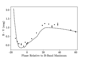
Figure 3: B-V color data of SN 2019ein compared with the color curve of the B15 model of Blondin, Dessart, & Hillier (2015) for the HV SN 2002bo (dashed line). Only LCO 1m photometry data obtained before +60 days are presented. For clarity, observations taken on the same day have been median combined. The data have been corrected for Milky Way extinction; neither the data nor the model have been corrected for host galaxy extinction.

Using our maximum-light photometry, we estimate the bolometric maximum luminosity and the corresponding ⁵⁶Ni mass. We follow the methods outlined in Howell et al. (2009): first, the measured flux at B-band maximum is calculated by integrating the magnitudes in U, g, r, and i filters to ensure optimal wavelength coverage of the optical region. In order to calculate the flux across the rest of the spectrum, we adopted the synthetic spectrum produced by the B15 model. As we show in Section 4.3, this model produces close fits to the spectrum of SN 2019ein at maximum light. We scale the B15 spectrum flux to match the distance of SN 2019ein. Next we scale the flux of the synthetic spectrum within our filter wavelength ranges to match the observed flux. We then divide this “warped” flux by the ratio of the measured flux to the total flux in the synthetic spectrum, and define this quantity to be the bolometric flux.

Following this procedure, we find a maximum bolometric luminosity of $L\sim 7.28\times 10^{42}$ erg s^-1. Using the relationship for the luminosity per ⁵⁶Ni mass $\dot{S}$ from Howell et al. (2009),

$$\dot{S}=6.31\times 10^{43}e^{t_{r}/8.8}+1.43\times 10^{43}e^{t_{r}/111}\text{ergs^{-1}M\odot^{-1}}$$ (1)

which is based on Arnett’s rule (Arnett, 1979), we calculate a ⁵⁶Ni mass of $\sim 0.33$ M_⊙ assuming a rise time of $\approx 16.5$ days. This mass is on the low end for SNe Ia (Stritzinger et al., 2006),but is supported by the analytic relationship found in Könyves-Tóth et al. (2020) between light-curve width and ⁵⁶Ni mass. Because SN 2019ein is a relatively fast decliner with $\Delta m_{15}(B)=$ 1.40 and is slightly subluminous ($M_{B}=$ -18.81), we conclude that this ⁵⁶Ni mass is a reasonable estimate.

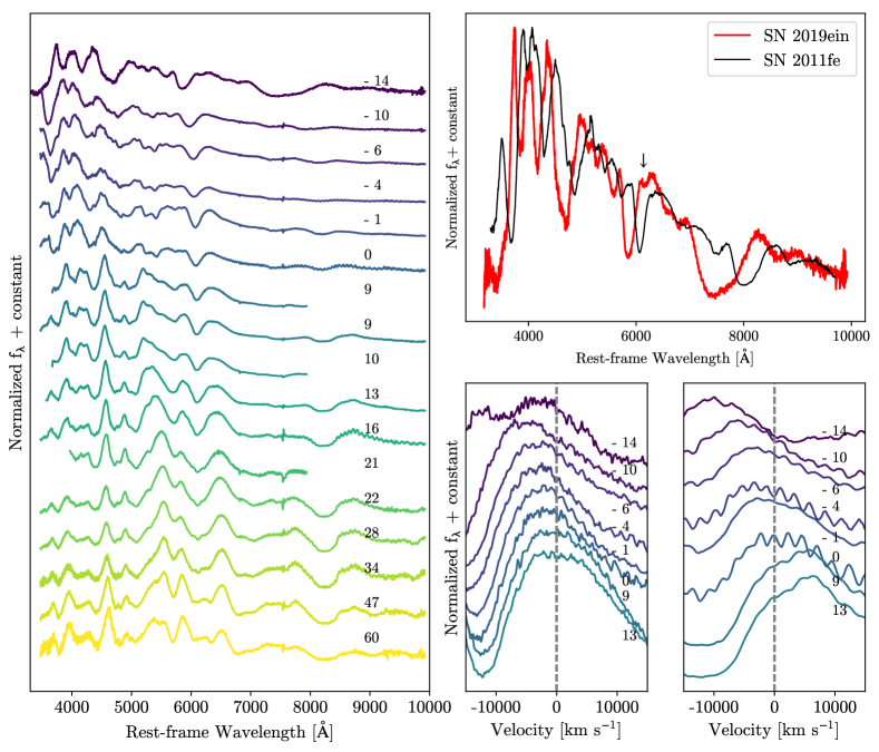
Figure 4: Left: the spectral evolution of SN 2019ein, from discovery 14 days before B-band maximum light until 60 days after B maximum. Spectra are described in Table 1. The phase with respect to B-band maximum is shown to the right of each spectrum. All fluxes are plotted on a linear scale. These spectra are available as Data behind the Figure. Top right: the spectrum of SN 2019ein at -14 days (red) compared with that of SN 2011fe at the same phase (black). A downward arrow denotes C II absorption in the spectrum of SN 2019ein. Bottom right: the emission components of the Si II 6355 Å (left) and Ca II NIR (right) P Cygni profiles from -14 days to 13 days with respect to B-band maximum light. The rest wavelengths of these features are shown with dashed lines. We caution that the apparent redshift of the Ca II NIR emission component after maximum light is most likely due to line overlap.

4 Spectroscopic Analysis

Figure 4 (left) shows the spectral evolution of SN 2019ein, from -14 to 60 rest-frame days with respect to B-band maximum light. In our earliest spectrum (Figure 4, top right) the most striking features include the broad absorption trough centered at approximately 7500 Å, which is most likely the result of blended Ca II and O I absorption at HVs ($>$ 30,000 km s^-1), as well as the broad Si II absorption centered at a wavelength less than 6000 Å. The Si II absorption minimum corresponds to a velocity of approximately 24,000 km s^-1, which is one of the highest velocities ever measured in a SN Ia (Gutierrez et al., 2016). Additionally, the Ca II H&K absorption feature is not well defined in this spectrum. This could be due to blending with other absorption lines, or it may be that the line is blueshifted outside of the sensitivity of our spectrograph, although such a blueshift would correspond to a seemingly unphysical velocity of $\sim$45,000 km s^-1. At this phase, the entire spectrum of SN 2019ein is noticeably blueshifted with respect to that of SN 2011fe. Before maximum light the blueshifts of the emission peaks remain prominent; the shifts are greatest in our first epoch, where both the Si II 6355 Å and Ca II NIR components are displaced with velocities upward of 10,000 km s^-1 (Figure 4, bottom right).

Also seen in the earliest spectrum is a small absorption notch, denoted with a black arrow, at a rest-frame wavelength of approximately 6150 Å. This feature is most likely C II 6580 Å at $\approx$ 20,000 km s^-1, as there is also a possible absorption feature from the C II 7235 Å line at the same velocity. Unburnt carbon in early-time spectra of SNe Ia is not unusual (e.g. Parrent et al. 2011; Blondin et al. 2012; Folatelli et al. 2012; Silverman & Filippenko 2012; Maguire et al. 2014); however, few SNe Ia show Si II 6355 Å absorption velocities higher than C II 6580 Å absorption velocities at early times (Parrent et al., 2011; Folatelli et al., 2012; Silverman & Filippenko, 2012), with a notable exception being SN 2011fe (Parrent et al., 2012; Pereira et al., 2013). The fact that SN 2019ein shows the opposite trend at this phase may shed light on the explosion mechanism and ejecta geometry. Parrent et al. (2011) note that $v_{\text{CII}}$/$v_{\text{SiII}}<1$ if the C II feature comes from an asymmetric ejecta distribution viewed at an angle with respect to the observer’s line of sight.

Close to B-band maximum, we note a possible HVF in the Ca II H&K line, as a weaker, lower velocity component becomes visible at roughly -4 days. However, HVFs usually develop at earlier phases, and this feature we observe is equally well fit by Si II absorption, making identification of HVFs at this phase difficult. Except for this exception, we do not find evidence for HVFs in the spectra of SN 2019ein, and all the velocities we report here are measured from the center of the dominant absorption feature for each line. The lack of two distinct absorption components sets SN 2019ein apart from most other HV SNe Ia. We discuss possible reasons for this difference in Section 6.

Using the MMT Observatory, we obtained a medium-resolution (R $\approx$ 3900) spectrum centered on the Si II 6355 Å absorption feature at +18 days with respect to B-band maximum (Figure 5). At this phase, the feature takes on an unusual asymmetric appearance. In particular, there appear to be multiple overlapping absorption troughs, each with a different line strength and Doppler shift. This may be caused by significant Si II mixing at this epoch, in which different distributions of Si II are moving at different velocities. This possibility is explored further in Section 6.

By approximately three weeks after maximum light, the Si II feature begins to blend with iron-group element (IGE) lines that dominate the spectrum. These IGE features, marked with black arrows, are most easily seen in the NIR spectrum obtained 32 days after B-band maximum, shown in Figure 6. Line blanketing from IGEs are seen in between the two telluric regions and at wavelengths greater than 2.0 $\mu$m. At this later phase, most C I and intermediate-mass element (IME) lines, usually seen around maximum light (e.g. Hsiao et al. 2013, 2015), have disappeared from the NIR spectrum.

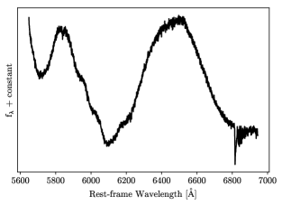
Figure 5: A medium-resolution spectrum of SN 2019ein, obtained with the MMT spectrograph at +18 days with respect to B-band maximum light, centered on the Si II 6355 Å absorption feature. Wavelengths have been shifted to the rest frame.

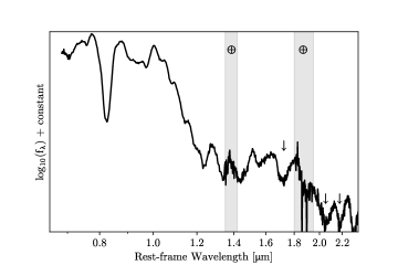
Figure 6: An NIR spectrum of SN 2019ein, obtained with the SpeX spectrograph via low-resolution PRISM mode on the NASA Infrared Telescope Facility at +32 days with respect to B-band maximum light. Wavelengths have been shifted to the rest frame and fluxes have been plotted in logarithmic units. The gray shaded regions denote wavelengths with strong telluric features, while black arrows denote possible IGE absorption features.

4.1 Branch Classification

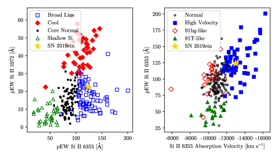
Figure 7: Left: pEW of Si II 5972 Å plotted against the pEW of Si II 6355 Å at B-band maximum light, according to Branch et al. (2006). Different Branch classifications are given by different colored symbols. SN 2019ein is shown with a gold star. Right: pEW of Si II 6355 Å versus Si II 6355 Å absorption velocity at B-band maximum light. Here different symbols correspond to different spectral subclasses of SNe Ia. Sample data are obtained from Blondin et al. (2012).

Branch et al. (2006) showed that the ratio of the pseudo-equivalent width (pEW) of the Si II 6355 Å absorption line to that of the Si II 5972 Å line can be used as a spectroscopic classification of SNe Ia. Here we classify SN 2019ein in the same way. We measure the pEWs with the following procedure: first, the spectrum is smoothed with a Savitzky-Golay filter to reduce the effects of noise. Next, the absorption feature of interest is defined and maxima blueward and redward of the absorption minimum along the continuum are found. We define the pseudo-continuum as simply the linear curve connecting the two maxima, so long as the curve does not intersect the spectral feature. Finally, the pEW is calculated using the formula (e.g. Garavini et al. 2007)

$$\text{pEW}=\sum_{i=0}^{N-1}\Delta\lambda_{i}\Bigg{(}\frac{f_{c}(\lambda_{i})-f(\lambda_{i})}{f_{c}(\lambda_{i})}\Bigg{)}$$ (2)

, where $f(\lambda_{i})$ is the measured flux, $f_{c}(\lambda_{i})$ is the flux of the pseudo-continuum, and $\Delta\lambda_{i}=\lambda_{i+1}-\lambda_{i}$ is the size of the wavelength bin at each wavelength interval $\lambda_{i}$.

At maximum light, we find that the pEW of Si II 6355 is 125 $\pm$ 2.1 Å and the pEW of Si II 5972 is 22.5 $\pm$ 2.8 Å. The corresponding Branch diagram is plotted in Figure 7. Compared to the sample from Blondin et al. (2012), SN 2019ein falls within the broad-line (BL) region of parameter space. This classification agrees with that presented in Kawabata et al. (2020). The right side of Figure 7 shows the pEW of Si II 6355 Å versus the velocity of the Si II 6355 Å absorption feature at maximum light, labeled by spectroscopic subtype. Here SN 2019ein lies within the population of HV SNe. Blondin et al. (2012) find a correlation between BL SNe and HV SNe, according to the Wang et al. (2009) classification scheme.

4.2 Absorption Velocities

SN 2019ein shows some of the highest expansion velocities of any SNe Ia in its early-time spectra. Velocities were calculated following the method outlined in Childress et al. (2014): first we select the absorption line of interest and define a pseudo-continuum by fitting a linear curve to the continuum maxima on both sides of the absorption trough. We normalize the flux with respect to this pseudo-continuum before fitting a Gaussian to the normalized absorption line. The minimum of the Gaussian is taken to be the Doppler-shifted observed wavelength, and the expansion velocity is calculated by comparing this measured absorption minimum to the known rest value of the line.

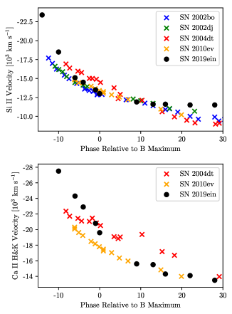
Figure 8: The Si II 6355 Å (top) and Ca II H&K (bottom) absorption velocity evolution from -14 days to 30 days for SN 2019ein, compared to a sample of other HV SNe (from Gutierrez et al. 2016).

Figure 8 compares the Si II 6355 Å and Ca II H&K absorption velocity evolution of SN 2019ein to several other HV SNe Ia from Gutierrez et al. (2016). These objects all show similar spectral features (Figure 9), including strong Ca II NIR absorption at early times, broad Si II 6355 Å absorption at maximum light, and HV Si II and Ca II before maximum. We do not report a Ca II H&K velocity -14 days with respect to B-band maximum light because at this epoch, no clear absorption minimum is identified within the wavelength range of our spectrograph.

The velocity evolution of all lines is rapid. The first epoch, corresponding to 14 days before maximum light and at most 3 days after explosion, shows the highest Si II velocity in this sample. By maximum light, the ejecta velocity remains high, yet falls within the range of the other HV SNe. After maximum light, we measure a velocity gradient to the Si II velocity following the example of Blondin et al. (2012), who found that measuring the change in Si II velocity between maximum light and $10\pm 2$ days after maximum gives the most consistent result. Using this method, we calculate a Si II velocity gradient $\dot{v}=122\pm 25$ km s^-1 day^-1, placing SN 2019ein in the HVG class (Benetti et al., 2005).

Figure 9: Spectra of SN 2019ein and four other HV SNe at -4 days with respect to B-band maximum light (from Gutierrez et al. 2016 and Altavilla et al. 2007).

4.3 Comparison to a Delayed-detonation Explosion Model

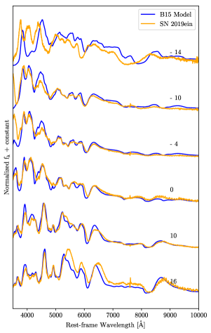
Figure 10: Spectra of SN 2019ein (orange) compared with the B15 synthetic spectra (blue; Blondin, Dessart, & Hillier 2015). Shown at the top right of every spectrum is the corresponding phase with respect to B-band maximum light.

Dessart et al. (2014) found that delayed-detonation explosions best model BL HVG SNe Ia. Additionally, Kawabata et al. (2020) found that the observed properties of SN 2019ein match those seen in the delayed-detonation models of Iwamoto et al. (1999). Figure 10 compares the spectra of SN 2019ein at various phases to delayed-detonation model spectra produced by Blondin, Dessart, & Hillier (2015). The B15 model simulates the spherically symmetric delayed-detonation of a Chandrasekhar-mass WD, imposed with radial mixing to match abundance stratifications observed in SNe ejecta, particularly those of IMEs and IGEs. Synthetic spectra from explosion to nearly 100 days after maximum light are produced.

Beginning 10 days before B-band maximum, the synthetic spectra match the strengths and velocities of most of the absorption features, including the Si II 6355 Å and Ca II NIR and H&K troughs. However, at our earliest epoch of -14 days, the spectrum of SN 2019ein significantly deviates from the B15 model spectrum at the same phase. The model fails to reproduce the extremely high absorption velocities, the broad mix of O I and Ca II NIR absorption, and the overall blueshift of the emission features with respect to the rest frame of the galaxy. The authors found similar discrepancies when they compared the earliest model spectra to the early-time spectra of SN 2002bo, and suggested that this may be due to underestimated outward mixing or a more complicated explosion than their one-dimensional, spherically symmetric model. Observational evidence for this enhancement of IMEs in the outer layers of the ejecta, possibly due to an extended burning front or significant mixing, was also found for SN 2002bo (Benetti et al., 2004) and the HV SN 2004dt (Altavilla et al., 2007).

In order to investigate the cause of this discrepancy, we now explore possible sources of the HV ejecta in SN 2019ein, including interaction with a circumstellar shell of material from the progenitor system or mixing and optical depth effects in the ejecta.

5 Progenitor Constraints from Radio Observations

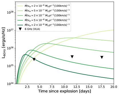
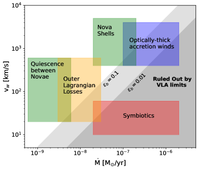
Figure 11: (a) 6 GHz radio light curves from the $r^{-2}$ wind model (Section 5.1) for different ratios of constant mass-loss rates ($\dot{M}$) and wind velocities ($v_{w}$). The 3$\sigma$ 6GHz VLA upper limits are shown as black triangles. (b) The parameter space of $\dot{M}-v_{w}$. The colored regions show approximate parameter spaces expected for different single-degenerate progenitor models as defined in Figure 3 of Chomiuk et al. (2012). The light and dark gray regions represent the parameter space of the $r^{-2}$ model that is ruled out by our VLA upper limits. These regions are defined by $\dot{M}/v_{w}>1.9\times 10^{-10}$ M_⊙ yr^-1 (km s^-1)^-1 assuming $\epsilon_{b}=0.1$, and $\dot{M}/v_{w}>9.5\times 10^{-10}$ M_⊙ yr^-1 (km s^-1)^-1 assuming $\epsilon_{b}=0.01$ (see Section 5.1 for details)

Radio emission is a sensitive probe of the progenitor environment (which we will refer to as circumstellar medium, or CSM). The CSM is modified by mass loss from the progenitor in the pre-SN stage, and interaction of the SN ejecta with this CSM accelerates electrons to relativistic energies and amplifies the ambient magnetic field, producing synchrotron radio emission (Chevalier, 1982, 1984, 1998). Simple models of radio emission have provided constraints on the CSM environment and progenitor properties for both core-collapse (e.g. Ryder et al., 2004; Chevalier & Fransson, 2006; Soderberg et al., 2006; Weiler et al., 2007; Salas et al., 2013) and SNe Ia (Panagia et al., 2006; Chomiuk et al., 2016). Radio emission is yet to be detected from a SN Ia, but nondetections have provided stringent constraints on progenitor scenarios (Chomiuk et al., 2016), particularly for nearby events such as SN 2011fe (Horesh et al., 2012; Chomiuk et al., 2012) and SN 2014J (Pérez-Torres et al., 2014). We can similarly interpret possible progenitor scenarios of SN 2019ein by comparing our VLA observations with models of radio emission from circumstellar interaction.

5.1 Wind Model ($\propto r^{-2}$)

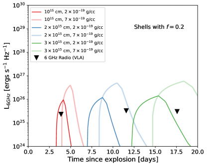
Figure 12: Light curves from the shell model of H16 for a shell of fractional width, $f=0.2$. The colors are for different shell radii, and the different shades are for different densities. The black triangles show the 3$\sigma$ upper limits from our VLA observations.

For single-degenerate progenitors, a fraction of the mass, transferred via accretion from a nondegenerate companion, is expected to be lost in the form of a wind. Chevalier (1982) created a simple parametric model of such a wind, characterized by a constant mass-loss rate ($\dot{M}$) and wind velocity ($v_{w}$), which leads to a CSM whose density ($\rho$) varies with radius ($r$) as

$$\rho=\frac{1}{4\pi r^{2}}\left(\frac{\dot{M}}{v_{w}}\right)$$ (3)

The synchrotron radio light curve from a shock propagating through such a CSM is described in Chevalier (1982) and Chevalier (1998). In this work, we follow the formalism of Chomiuk et al. (2016) (hereafter C16), who adopted the self-similar solutions of Chevalier (1982) for radio observations of SNe Ia. We assume a Chandrasekhar-mass WD progenitor that exploded with 10⁵¹ erg of kinetic energy, consistent with our optical observations, and a steep outer ejecta profile of $\rho_{ej}\sim v_{ej}^{-10}$ interacting with the above CSM. Electrons are accelerated to a power-law spectrum ($\sim E^{-p}$, with $p=3$). The average fraction of the shock energy shared by the cosmic-ray electrons and the amplified magnetic field in the shock vicinity is parameterized as $\epsilon_{e}$ and $\epsilon_{b}$ respectively. As in Chomiuk et al. (2012) and Chomiuk et al. (2016), we set $\epsilon_{e}=0.1$ and $\epsilon_{b}=[0.1,0.01]$, consistent with values expected in Type Ib/c SNe (Chevalier & Fransson, 2006; Sironi & Spitkovsky, 2011; Soderberg et al., 2012).

The light-curve models for different values of the free parameters $\dot{M}$ and $v_{w}$ are shown in Figure 11. The rising part of the light curves corresponds to the regime where the ejecta are still optically thick to synchrotron self-absorption at 5 GHz. When the ejecta are optically thin, the light curve declines. Higher ratios of $\dot{M}/v_{w}$ correspond to denser outflows, which leads to brighter light curves and a delayed transition to the optically thin stage, which explains why the peaks are shifted to later epochs.

Figure 11 shows our constraints on the $\dot{M}/v_{w}$ parameter space from the VLA upper limits in Section 2.1. We are able to rule out the parameter space for $\dot{M}/v_{w}>1.9\times 10^{-10}$ M_⊙ yr^-1 (km s^-1)^-1 for $\epsilon_{e}=\epsilon_{b}=0.1$. For $\epsilon_{e}=0.1$ and $\epsilon_{b}=0.01$, we find that $\dot{M}/v_{w}>9.5\times 10^{-10}$ M_⊙ yr^-1 (km s^-1)^-1.

The above constraints on $\dot{M}/v_{w}$ can provide some insight into possible single-degenerate progenitor models for SN 2019ein by comparing with typical values of $\dot{M}$ and $v_{w}$ expected in these models as compiled in Chomiuk et al. (2012). Our observations are sensitive enough to rule out symbiotic progenitors, i.e. a WD that accretes from the wind of a giant companion, which is generally characterized by $\dot{M}>10^{-8}$ M_⊙ yr^-1 and $v_{w}\approx 30$ km s^-1 (Seaquist & Taylor, 1990; Chen et al., 2011; Patat et al., 2011). A symbiotic channel was also deemed unlikely for the nearest events SN 2011fe and SN 2014J, and was found to contribute no more than $16\%$ of a sample of 85 SNe Ia with available radio observations studied by (Chomiuk et al., 2016). For $\epsilon_{e}=0.1$ and $\epsilon_{b}=0.01$, our increased upper limit of $\dot{M}/v_{w}>9.5\times 10^{-10}$ M_⊙ yr^-1 (km s^-1)^-1 still excludes the majority of symbiotic progenitors observed in the Galaxy (Seaquist et al., 1993; Chomiuk et al., 2016).

White dwarfs can also be in single-degenerate systems with a main-sequence or a slightly evolved companion undergoing mass transfer via Roche-lobe overflow. For mass accretion rates $\gtrsim 3\times 10^{-7}$ M_⊙ yr^-1, steady nuclear burning occurs on the surface of the WD, and about $\sim 1\%$ of the mass is lost from the outer Lagrangian point with velocities of about a few 100 km s^-1 (Shen & Bildsten, 2007). The expected $\dot{M}/v_{w}$ in such a scenario falls within our VLA limits, and therefore such a progenitor channel cannot be ruled out for SN 2019ein from our radio observations alone. With increasing accretion rate, however, the nuclear burning shell will drive fast optically thick winds with $v_{w}\approx$ few $\times 1000$ km s^-1 (Hachisu et al., 1999), and some part of this parameter space is ruled out by our VLA upper limits. For accretion rates $\approx(1-3)\times 10^{-7}$ M_⊙ yr^-1, the steady burning will be interrupted by recurrent nova flashes. Novae with short recurrence time will likely create a series of dense shells with which the SN shock will interact, and such shells typically have values of $\dot{M}$ and $v_{w}$ as shown in Figure 11. For longer recurrence times, the SN shock is more likely to interact with CSM created with a steady wind with $\dot{M}\approx 10^{-9}-10^{-8}$ M_⊙ yr^-1 in between distant novae shells (Wood-Vasey, & Sokoloski, 2006). Both these cases are allowed within our upper limits in the context of the $r^{-2}$ model, but we will also analyze the presence of nova shells with a more appropriate shell-interaction model in Section 5.2.

We note here the importance of radio observations taken soon after explosion or discovery for SNe Ia. The first observation, which was triggered $<2$ days of discovery and $\lesssim 4$ days of explosion, provided a constraint that is almost a factor of five deepert on $\dot{M}/v_{w}$ than the observation a week later (Figure 11). This is because lower $\dot{M}/v_{w}$ shifts the peak of the radio light curve to earlier times, as seen in Figure 11. The prompt observation resulted in more stringent constraints on Type Ia progenitor models involving symbiotic systems and optically thick winds.

5.2 Shell Interaction Model

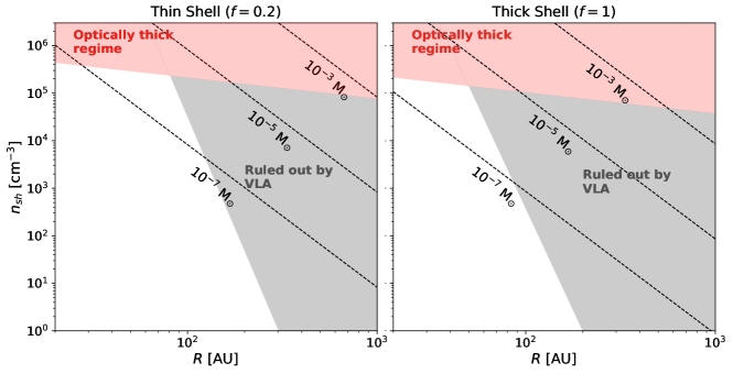
Figure 13: Parameter space of the CSM shell radii $R$ versus shell density $n_{h}=\rho_{sh}/\mu m_{p}$, where $\rho_{sh}$ is the density in units of g cm^-3, $\mu=1.4$, and $m_{p}=1.67\times 10^{-24}$ g. Dashed lines in both panels correspond to lines of constant shell mass $M_{sh}=4/3\pi\rho_{sh}R^{3}[(1+f)^{3}-1]$. The left panel corresponds to a thin shell, while the right panel corresponds to a thick shell. The gray shaded region is the parameter space where the H16 light curves are inconsistent with the constraints described in Section 5.2. The red shaded region is where optical depth due to synchrotron self-absorption is $>1$ and the optically thin ejecta assumption of H16 is no longer valid.

Interaction and acceleration of material in solar-composition CSM shells has been proposed as a way to explain HVFs in Type Ia spectra (Gerardy et al., 2004; Mulligan, & Wheeler, 2018; Mulligan & Wheeler, 2017). Such shells can be expected in WD progenitors that undergo nova outbursts. Shells can consist of recently ejected material or of swept-up material from previous outbursts. Shock interaction with such a shell can produce detectable radio emission, and radio light curves for such a CSM created by discrete mass-loss events cannot be appropriately described by a continuous mass-loss model.

We therefore use the models described in Harris et al. (2016), hereafter H16, for radio emission from a CSM shell interacting with SN ejecta. H16 performed hydrodynamical simulations of a $\rho_{ej}\sim v_{ej}^{-10}$ ejecta profile interacting with a single, solar-metallicity, fully ionized shell defined by an inner radius $R$, fractional width $f=\Delta R/R$, and constant shell density $\rho_{sh}$. Interaction creates a forward shock in the shell and a reverse shock in the ejecta, but the dynamics do not reach self similarity, unlike in the Chevalier (1982) case. The forward shock subsequently accelerates the CSM and sets it in free expansion.

In the optically thin approximation, the H16 light-curve model can be analytically expressed in terms of $f,\rho_{sh}$ and $R$ (see Eqs. 5-13 in H16). Figure 12 shows example light curves from the H16 model. The light curves are characterized by a rapid brightening at the beginning of the interaction, reaching a peak luminosity when the forward shock reaches the outer edge of the CSM shell, and a steep decline once the shock breaks out. For larger $f$, the light curves peak at later times because the shock takes longer to reach the CSM outer edge. For larger $R$, the light curves begin at a later time, and larger $\rho_{sh}$ produces brighter light curves.

Similar to the analysis in Cendes et al. (2020), we explore the parameter space of $R$-$\rho_{sh}$ for a given $f$ that produces light curves within our VLA upper limits at the observed epochs. We explore two cases of shells: a thin shell ($f=0.2$) characteristic of shells expected in nova eruptions, and a thick shell ($f=1$) to show the effects of increasing shell width. Similar to the wind model, the shell models assume a standard Chandrasekhar-mass WD explosion with 10⁵¹ erg of kinetic energy, and $\epsilon_{e}=\epsilon_{b}=0.1$. We also use an additional constraint: the peak of the light curve must occur before the first epoch (i.e. at 3.87 days after explosion). This is because any shell interaction leading to HV absorption features must have occurred before the first spectral observation (i.e. after the shell has been accelerated by the forward shock, Gerardy et al., 2004).

Figure 13 shows the result of applying the H16 shell models to our VLA observations. For our fiducial model parameters in both the thin and thick shell cases, the VLA limits only allow CSM shells $\lesssim 10^{-6}$ M_⊙ within radii $<100$ AU. In comparison, CSM masses $\sim 10^{-3}-10^{-2}$ M_⊙ are generally required to explain HVFs observed in SNe Ia (Gerardy et al., 2004). We note that this conclusion remains unchanged even when we assume $\epsilon_{b}=0.01$ because the shaded region in Figure 13 is determined primarily by the condition that the peak of the light curve must occur before the first epoch, as mentioned previously. As explained in H16, the light curve peaks when the shock reaches the outer edge of the shell and is thus mainly a hydrodynamical timescale, which is independent of the parameter $\epsilon_{b}$ that affects only the radio emission.

A caveat, however, is that the H16 model approximates the radio emission as optically thin, whereas at densities $>10^{5}$ cm^-3 for the radii explored here, effects such as synchrotron self-absorption, free-free absorption, and radiative cooling of the shock gas will become important. Light-curve models in this optically thick regime would require a formal solution of the radiative transfer equation, which will be explored in an upcoming paper (C. E. Harris et al. 2020, in preparation), and will help provide more accurate constraints on the presence of dense and massive CSM shells.

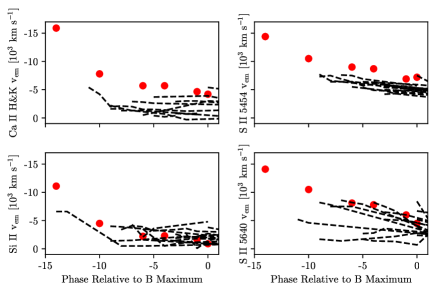
Figure 14: The emission peak Ca II H&K (top left), Si II 6355 Å (bottom left), S II 5454 Å (top right), and S II 5640 Å (bottom right) velocities of SN 2019ein, shown in red, compared against the low-redshift sample from Blondin et al. (2006), shown in dashed black, from -14 days to 0 days with respect to B-band maximum light.

6 Mixing and Optical Depth Effects

The high emission velocities before maximum light make SN 2019ein unusual, even among HV SNe Ia. More specifically, although P Cygni emission blueshifts have been theoretically predicted and observed in Type II SNe (Dessart & Hillier, 2005) and were discussed by Blondin et al. (2006) in a sample of low-redshift SNe Ia, the emission velocities seen in the spectra of SN 2019ein are the highest ever measured. Figure 14 shows the evolution of the emission velocities for four lines in the spectra of SN 2019ein compared to the sample from Blondin et al. (2006). It is clear that at early times, the emission peaks in SN 2019ein are substantially more blueshifted than in any of the objects in the comparison sample. This extreme behavior is most clearly seen in the plots of the Ca II H&K and S II emission velocities, where the emission velocities at -14 days with respect to B-band maximum are $\approx$ 15,000 km s^-1. At the same phase, the Si II emission component of the P Cygni profile is blueshifted by $\approx$ 10,000 km s^-1. Even around maximum light, the velocities of these lines are among the highest ever measured. After maximum, the emission peaks are either no longer resolvable or become distorted due to line overlap, possibly of multiple Doppler-shifted emission features (see Figure 5). Here we only present emission velocities up to B-band maximum, where we trust our measurements have not been biased.

In order to investigate whether specific ejecta compositions or abundance enhancements could cause both the high absorption and emission velocities at early times, we compare SYN++ (Thomas, Nugent, & Meza, 2011) model spectra to our spectrum of SN 2019ein at -10 days. In particular, we focus on the Si II 6355 Å feature and test whether multiple components of the ejecta, such as a HV component with a velocity above the photospheric velocity (PV), can reproduce the measured Doppler shifts.

Our synthetic spectrum is shown in Figure 15 compared to our spectrum of SN 2019ein at -10 days. We find that an ejecta with only a HV Si II component offset from the PV by several thousand km s^-1 provides the best fit to our data. This matches the lack of separate HVFs and PVFs, particularly in the Si II and Ca II lines, at early times in our observed spectra, as well as the analysis of our radio observations, which places stringent constraints on the mass of a CSM shell, which has been proposed to produce HVFs. Altogether, this indicates that only a HV Si II component is present in the ejecta of SN 2019ein. We attempt to explain the existence of this HV component as being due to ejecta mixing from an asymmetric explosion or being caused by optical depth effects in the outer layers of the ejecta.

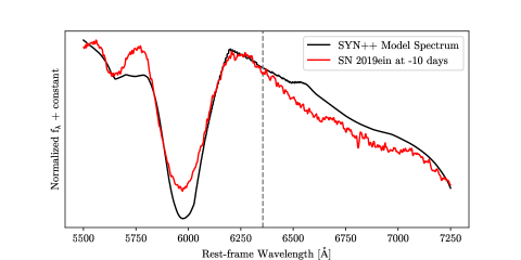
Figure 15: SYN++ synthetic spectrum (black) of the Si II 6355 Å feature at -10 days with respect to B-band maximum, compared to the spectrum of SN 2019ein at the same epoch (red). Our synthetic spectrum contains only a HV Si II component offset from the photospheric velocity by 2,500 km s^-1. The rest wavelength of the Si II emission peak is represented by a dashed vertical line.

6.1 Evidence for Asymmetries

In Section 4.3 we discuss that objects similar to SN 2019ein exhibit significant mixing of their IMEs to higher velocities. This may be evidence of an aspherical ejecta distribution due to an asymmetric explosion, in which clumps of IMEs are mixed to higher velocities along the observer’s line of sight, producing HV absorption and emission features. Similar clumps are produced in models of off-center delayed-detonation explosions (Seitenzahl et al., 2013). The connection between mixing and asymmetries has observational support. Polarization measurements show that HVFs in SNe ejecta are more polarized than PVFs, indicating that HV ejecta have more asymmetric distributions (Maund et al., 2013; Bulla et al., 2016). Additionally, Nagao et al. (2019) observed high polarization alongside a blueshift of the H$\alpha$ line during the photospheric phase of the Type II SN 2017gmr.

There is evidence for such an aspherical ejecta distribution in the spectra of SN 2019ein; in the early-time spectra of SN 2019ein, we see Si II with a higher absorption velocity than C II at -14 days, whereas the opposite relation is true at this phase for the SNe studied by Parrent et al. (2011). In a spherically symmetric model of a Type Ia explosion, the inner burning regions are surrounded by a shell of unburnt material comprised mostly of C and O. However, an asymmetric explosion with strong outward mixing could force IMEs produced in the nuclear burning to higher velocities. In addition, our medium-resolution spectrum obtained 18 days after B-band maximum light reveals multiple overlapping Si II absorption features, with each absorption minimum offset by several thousand km s^-1. This may be evidence of significant mixing of the Si II ejecta to lower and higher velocities, rather than the stratified shell-like structure proposed in studies of other SNe Ia (Cain et al., 2018).

Studying the nebular-phase spectroscopy of SNe Ia, Maeda et al. (2010) found a relationship between the Doppler shift of the nebular-phase emission features and the Si II velocity gradient at early times, whereby HVG SNe exhibit redshifted nebular-phase emission lines and LVG SNe show blueshifted nebular emission lines. This correlation is suggested to detail information about the symmetry of the explosion because the nebular-phase emission features trace the deflagration ash in the core of the progenitor WD. In this model, HVG SNe are viewed from the direction opposite to the initial deflagration.

Finally, Maund et al. (2010) and Cikota et al. (2019) found correlations between the Si II line polarization and velocity evolution around maximum, with more polarized SNe belonging to the HV and HVG classes. Maund et al. (2010) argue that this relationship implies the existence of global asymmetries in the ejecta, which, along with the correlation between velocity evolution and nebular-phase velocity shifts (Maeda et al., 2010), connects early- and late-time velocity behavior to the three-dimensional geometry of the explosion. It is possible that the high absorption and emission velocities seen in the spectra of SN 2019ein are signatures of IMEs in the ejecta that were outwardly mixed in an off-center explosion.

6.2 Optical Depth Effects

Blueshifted emission features have been suggested to be caused by optical depth effects in Type II SNe (e.g. Dessart & Hillier 2005, 2011; Anderson et al. 2014). These features arise from steep density profiles in the expanding ejecta (see Figure 16 in Dessart & Hillier 2005). Blondin et al. (2006) were the first to model these features in SNe Ia. Using the radiative transfer code CMFGEN (Hillier & Miller, 1998), the authors found that differences in optical depths of Si II and S II lines resulted in overall blueshifted emission peaks when the flux was integrated over a range of impact parameters.

In this picture, contours of constant optical depth in the photosphere trace out a variable amount of the emitting ejecta, where the amount of emission from the ejecta above the photosphere depends on the optical depth of the line being considered. In the classical P Cygni profile, the flux from the ejecta moving perpendicular to the observer’s line of sight makes up the majority of the emission, resulting in an emission peak centered on the rest wavelength of the line. However, when lines with low optical depth are considered, there is little to no emission from the ejecta at large impact parameters because the density gradient in the outer ejecta layers is steep. Instead, the flux is dominated by ejecta moving toward the observer even if the ejecta is distributed more or less spherically. The result is an overall blueshift of the emission peak, proportional to the ejecta velocity. Because the authors modeled individual lines, the emission blueshifts cannot be the result of line overlap.

As seen in Figure 14, SN 2019ein has some of the highest emission peak velocities at early times compared to the sample from Blondin et al. (2006). This extreme behavior can be understood in the context of the above explanation: because blueshifted emission is dominated by flux from the ejecta moving toward the observer, we would expect that the emission velocity is correlated with the absorption velocity. Blondin et al. (2006) found that this trend exists, with the ratio of v_peak to v_abs approaching 0.6 around -10 days relative to B-band maximum for the S II 5454 Å line. Over time, the photosphere quickly recedes from the low-density material and the emitting region becomes more spherical, causing this ratio to approach 0 around B-band maximum light. However, at early times the photosphere is very far out in the ejecta, so the emitting ejecta we observe must be at HVs, leading to a greater emission peak blueshift. Our SYN++ spectrum supports this picture; the blueshift of the Si II 6355 Å emission peak is proportional to the Si II ejecta velocity. Because SN 2019ein has some of the highest absorption velocities measured at its earliest phases, the emission velocities of those lines are among the highest as well.

6.3 Discussion

We find that the high absorption and emission velocities at early times can be explained by an HV-only ejecta component, possibly due to mixing in an asymmetric explosion or optical depth effects in the outer layers of the ejecta. It is possible that both effects are at play; the models of Maeda et al. (2010) predict that the outer regions of the SN ejecta on the side opposite from an off-center ignition are less dense and produce HVG SNe. It could be that in this lower density environment, the ejecta is optically thinner, leading to a majority of the flux stemming from material moving along the observer’s line of sight and producing blueshifted emission features.

Another nearby SN Ia with a well-studied density structure is SN 2012fr (Childress et al., 2013; Maund et al., 2013; Contreras et al., 2018). Cain et al. (2018) found that SN 2012fr showed signs of a shell-like density enhancement at low velocities, which could explain the unusual Si II velocity evolution as well as the presence of separate HV and PV features. However, SN 2012fr and similar SNe Ia tend to be slow decliners ($\Delta m_{15}\lesssim 1$), HV yet LVG, and fall outside the BL region of the Branch diagram (Contreras et al., 2018). These classifications are at odds with those we present for SN 2019ein. Therefore we suggest that SN 2019ein most likely has a different density enhancement than the shell-like structure of SN 2012fr.

One potential bias in our measurements is line blanketing. Line blanketing can warp the shape of the emission peaks, potentially biasing measurements of the peak wavelength. As noted by Branch et al. (2007), synthetic spectra rarely if ever produce the significant emission peak Doppler shifts around maximum light observed by Blondin et al. (2006) and again here in SN 2019ein. However, synthetic spectra also rarely produce only HV ejecta components, as we have done in our SYN++ model. Furthermore, the observed emission shifts are not seen in just one line but globally, and seem to follow a similar evolution over time. This can be seen in the comparison between the B15 model spectra and the real data in the earliest epoch (Figure 10). Therefore we conclude that line blanketing is unlikely able to reproduce the peculiar emission blueshifts at all wavelengths and phases.

Future observations will be necessary to provide more conclusive results on the geometry of the ejecta. For example, measuring a Doppler shift of the nebular-phase emission peaks could support the argument that SN 2019ein has signatures of an aspherical explosion. In addition, early-time polarimetry data would provide an additional measurement of the asymmetries in both specific spectral features, such as the Si II absorption line, and globally via the continuum polarization. However, as discussed by Dessart & Hillier (2011) and Kasen & Plewa (2007), low continuum polarization does not necessarily imply that the explosion was spherically symmetric; both authors find that even in models with significant asphericity, the line and continuum polarization could be low due to density and ionization effects. In the case of some geometries presented in Dessart & Hillier (2011) both an emission blueshift and a low polarization signal are produced, regardless of the underlying symmetry of the ejecta.

It is reasonable to question why SN 2019ein is so unusual, even in a sample of other BL HV SNe. One possible explanation is early-time observations; it is possible that SN 2019ein was first observed mere hours after explosion, allowing us to see the extremely high absorption and emission velocities at an earlier phase than other HV SNe. Another explanation is that SN 2019ein was observed from a rare viewing angle, as would be the case if the explosion were strongly asymmetric. Either way, the analysis of early-time photometry and spectroscopy presented here demonstrates the importance of finding and observing SNe Ia quickly after explosion.

7 Summary

We have presented photometric and spectroscopic observations of SN 2019ein, a SN Ia with some of the highest early-time ejecta velocities ever measured. We observe a Si II 6355 Å absorption velocity of 24,000 km s^-1 14 days before B-band maximum light. In addition, the early-time emission components of the P Cygni profiles appear blueshifted with respect to the host galaxy redshift, with emission peaks of Si II, Ca II, and S II moving at velocities up to or above 10,000 km s^-1. This emission blueshift is also among the highest ever measured, making SN 2019ein an outlier even among other HV SNe.

Radio observations taken as early as $<$4 days after explosion provide insight into the progenitor system of SN 2019ein as well as the source of the HV ejecta. Our 3$\sigma$ VLA upper limits of 18, 25, and 23 $\mu$Jy at 3.87, 11.57, and 17.58 days after explosion are sensitive enough to rule out symbiotic progenitors for SN 2019ein. We also rule out part of the parameter space of a single-degenerate model involving accretion from a main-sequence or slightly evolved companion at accretion rates $>3\times 10^{-7}$M_⊙ yr^-1, because the resulting fast optically thick winds would likely have created detectable circumstellar material. Such progenitor scenarios were also ruled out for the nearest and best-studied SNe Ia 2011fe and 2014J. Our upper limits cannot rule out models of a WD accreting at lower rates $\sim(1-3)\times 10^{-7}$ M_⊙ from a main-sequence or slightly evolved companion via winds that are sometimes interrupted by recurrent nova flashes. With our shell-interaction model (Harris et al., 2016) we can rule out the presence of optically thin shells, which have been theoretically predicted to source HV ejecta, of masses $>10^{-6}$ M_⊙ at distances $<100$ AU from the progenitor. However, denser or more massive shells in the optically thick regime cannot be ruled out by the current model, and will be revisited in the future with a more sophisticated shell model that takes synchrotron self-absorption and radiative losses into account.

We find that SN 2019ein is well fit by a delayed-detonation explosion model (Blondin, Dessart, & Hillier, 2015) except at early times, where our measured ejecta velocities are even higher than those predicted. By modeling the early spectra of SN 2019ein, we find that both the high absorption and emission velocities may be due to a HV component of the ejecta that is detached from the photosphere. This detached component of the ejecta may be evidence of an aspherical distribution of intermediate-mass elements, perhaps due to mixing in an asymmetric explosion (Seitenzahl et al., 2013). Additionally, optical depth effects in the very outer layers of the ejecta may lead to an overall blueshift in the spectrum, as the majority of the flux observed comes from material moving along the observer’s line of sight. These results highlight the need for more detailed modeling of SN ejecta, especially at early times.

By studying a larger sample of HV SNe Ia, we can begin to probe the overlap between explosion models, asymmetries, and ejecta velocities. Results from such a sample would have implications on theories of Type Ia progenitor systems and explosion mechanisms. It is possible that a united picture will emerge, one in which the ejecta geometry and the viewing angle to a SN affect observables such as color, velocity, and light-curve width. A similar intrinsic difference has already been noted in the colors and host environments of HV and Normal SNe (Wang et al., 2013; Zheng, Kelly, & Filippenko, 2018), and may be used to reduce uncertainties in Type Ia distances, improving the precision of cosmological measurements.

Appendix A Photometry Tables

Here we present tables of the optical photometry (Table 4), Swift UVOT photometry (Table 5), and NIR photometry (Table 6) of SN 2019ein.

Table 4: Optical Photometry of SN 2019ein

MJD	U	B	V	g	r	i
58607.9	15.6623$\pm$0.0178	16.2245$\pm$0.0068	16.0277$\pm$0.0094	16.0779$\pm$0.0069	16.0746$\pm$0.0083	16.3184$\pm$0.0123
58607.9	15.6691$\pm$0.0182	16.1875$\pm$0.0077	16.0273$\pm$0.0095	16.0761$\pm$0.0067	16.0725$\pm$0.0083	16.3133$\pm$0.0133
58609.9	14.9546$\pm$0.045	15.459$\pm$0.0246	15.3038$\pm$0.0066	15.2826$\pm$0.0049	15.2625$\pm$0.0055	15.4542$\pm$0.0074
58609.9	15.2438$\pm$0.0428	15.3734$\pm$0.0089	15.3246$\pm$0.0058	15.2677$\pm$0.0048	15.25$\pm$0.0045	15.4743$\pm$0.0074
58612.8	14.203$\pm$0.0131	14.6844$\pm$0.0071	14.6623$\pm$0.0059	14.5386$\pm$0.0163	14.5182$\pm$0.0064	-
58612.8	14.1956$\pm$0.0125	14.69$\pm$0.0081	14.5789$\pm$0.0068	-	14.5123$\pm$0.0074	-

Note. — This table is available in its entirety in machine-readable format.

Table 5: Swift UVOT Photometry of SN 2019ein

MJD	UVW2	UVM2	UVW1	U	B	V
58606.5	19.924$\pm$0.342	-	18.398$\pm$0.173	16.675$\pm$0.09	16.735$\pm$0.074	16.37$\pm$0.096
58607.8	18.801$\pm$0.16	20.359$\pm$0.35	17.559$\pm$0.11	15.727$\pm$0.068	16.103$\pm$0.063	15.698$\pm$0.073
58608.8	18.3$\pm$0.122	20.517$\pm$0.36	16.903$\pm$0.083	15.143$\pm$0.057	15.728$\pm$0.059	15.474$\pm$0.067
58609.8	18.069$\pm$0.111	20.292$\pm$0.302	16.512$\pm$0.074	14.816$\pm$0.051	15.242$\pm$0.049	15.159$\pm$0.063
58612.6	17.119$\pm$0.09	18.836$\pm$0.208	15.603$\pm$0.06	-	-	-
58616.1	16.71$\pm$0.076	18.099$\pm$0.118	15.321$\pm$0.06	13.855$\pm$0.043	14.189$\pm$0.042	14.037$\pm$0.049
58617.4	16.667$\pm$0.069	-	-	-	-	-
58617.4	16.642$\pm$0.078	-	-	-	-	-
58619.2	16.701$\pm$0.091	17.665$\pm$0.146	15.329$\pm$0.061	-	-	-
58620.2	16.681$\pm$0.074	17.795$\pm$0.093	15.423$\pm$0.06	14.096$\pm$0.044	14.152$\pm$0.042	13.843$\pm$0.047
58629.4	17.814$\pm$0.07	-	-	-	-	-
58629.4	17.568$\pm$0.105	-	-	-	-	-
58630.3	17.796$\pm$0.097	18.718$\pm$0.149	-	-	-	-
58702.2	20.162$\pm$0.347	-	-	18.175$\pm$0.173	17.536$\pm$0.094	16.956$\pm$0.119
58712.1	20.262$\pm$0.361	-	19.144$\pm$0.246	18.219$\pm$0.166	17.86$\pm$0.104	17.12$\pm$0.122

Table 6: NIR Photometry of SN 2019ein

MJD	J	H	Ks
58606.8	15.97$\pm$0.20	15.40$\pm$0.31	15.31$\pm$0.29
58606.9	15.91$\pm$0.22	15.56$\pm$0.28	15.32$\pm$0.32
58612.9	14.50$\pm$0.17	14.61$\pm$0.23	14.41$\pm$0.27
58617.8	14.29$\pm$0.24	14.50$\pm$0.24	14.24$\pm$0.30

References

- Altavilla et al. (2007) Altavilla, G., Stehle, M., Ruiz-Lapuente, P., et al. 2007, A&A, 475, 585
- Anderson et al. (2014) Anderson, J. P., Dessart, L., Gutierrez, C. P., et al. 2014, MNRAS, 441, 671
- Arnett (1979) Arnett, W. D. 1979, ApJ, 230, L37
- Bellm et al. (2019) Bellm, E. C., Kulkarni, S. R., Graham, M. J., et al. 2019, PASP, 131, 018002
- Benetti et al. (2004) Benetti, S., Meikle, P., Stehle, M., et al. 2004, MNRAS, 348, 261
- Benetti et al. (2005) Benetti, S., Cappellaro, E., Mazzali, P. A., et al. 2005, ApJ, 623, 1011
- Betoule et al. (2014) Betoule, M., Kessler, R., Guy, J., et al. 2014, A&A, 568, A22
- Blondin et al. (2006) Blondin, S., Dessart, L., Leibundgut, B., et al. 2006, AJ, 131, 1648
- Blondin et al. (2012) Blondin, S., Matheson, T., Kirshner, R. P., et al. 2012, AJ, 143, 126
- Blondin, Dessart, & Hillier (2015) Blondin, S., Dessart, L., & Hillier, D. J. 2015, MNRAS, 448, 2766
- Bloom et al. (2012) Bloom, J. S., Kasen, D., Shen, K. J., et al. 2012, ApJ, 744, L17
- Branch et al. (2006) Branch, D., Dang, L. C., Hall, N., et al. 2006, PASP, 118, 560
- Branch et al. (2007) Branch, D., Troxel, M. A., Jeffery, D. J., et al. 2007, PASP, 119, 709
- Breeveld et al. (2011) Breeveld, A. A., Landsman, W., Holland, S. T., et al. 2011, in AIP Conf. Ser. 1358, AIP Conf. Ser., ed. J. E. McEnery, J. L. Racusin, & N. Gehrels (Melville, NY: AIP), 373
- Brown et al. (2013) Brown, T. M., Baliber, N., Bianco, F. B., et al. 2013, PASP, 125, 1031
- Brown et al. (2014) Brown, P. J., Breeveld, A. A., Holland, S., et al. 2014, Ap&SS, 354, 89
- Brown et al. (2018) Brown, P. J., Perry, J. M., Beeny, B. A., et al. 2018, ApJ, 867, 56
- Bulla et al. (2016) Bulla, M., Sim, S. A., Kromer, M., et al. 2016, MNRAS, 462, 1039
- Burke et al. (2019) Burke, J., Arcavi, I., Howell, D. A., et al. 2019, ATel, 12719, 1
- Cain et al. (2018) Cain, C., Baron, E., Phillips, M. M., et al. 2018, ApJ, 869, 162
- Cendes et al. (2020) Cendes, Y., Drout, M. R., Chomiuk, L., et al. 2020, ApJ, 894, 39
- Chen et al. (2011) Chen, X., Han, Z., & Tout, C. A. 2011, ApJ, 735, L31
- Chevalier (1982) Chevalier, R. A. 1982, ApJ, 259, 302
- Chevalier (1984) Chevalier, R. A. 1984, ApJ, 285, L63
- Chevalier (1998) Chevalier, R. A. 1998, ApJ, 499, 810
- Chevalier & Fransson (2006) Chevalier, R. A., & Fransson, C. 2006, ApJ, 651, 381
- Childress et al. (2013) Childress, M. J., Scalzo, R. A., Sim, S. A., et al. 2013, ApJ, 770, 29
- Childress et al. (2014) Childress, M. J., Filippenko, A. V., Ganeshalingam, M., et al. 2014, MNRAS, 437, 338
- Chomiuk et al. (2012) Chomiuk, L., Soderberg, A. M., Moe, M., et al. 2012, ApJ, 750, 164
- Chomiuk et al. (2016) Chomiuk, L., Soderberg, A. M., Chevalier, R. A., et al. 2016, ApJ, 821, 119
- Cikota et al. (2019) Cikota, A., Patat, F., Wang, L., et al. 2019, MNRAS, 490, 578
- Contreras et al. (2018) Contreras, C., Phillips, M. M., Burns, C. R., et al. 2018, ApJ, 859, 24
- Cornwell et al. (2008) Cornwell, T. J., Golap, K., & Bhatnagar, S. 2008, IEEE Journal of Selected Topics in Signal Processing, 2, 647
- Dessart & Hillier (2005) Dessart, L. & Hillier, D. J. 2005, A&A, 439, 671
- Dessart & Hillier (2011) Dessart, L. & Hillier, D. J. 2011, MNRAS, 415, 3497
- Dessart et al. (2014) Dessart, L., Blondin, S., Hillier, D. J., et al. 2013, MNRAS, 441, 532
- Filippenko et al. (1992b) Filippenko, A. V., Richmond, M. W., Branch, D., et al. 1992, AJ, 104, 1543
- Filippenko et al. (1992a) Filippenko, A. V., Richmond, M. W., Matheson, T., et al. 1992, ApJ, 384, L15
- Fink et al. (2010) Fink, M., Röpke, F. K., Hillebrandt, W., et al. 2010, A&A, 514, A53
- Folatelli et al. (2012) Folatelli, G., Phillips, M. M., Morrell, N., et al. 2012, ApJ, 745, 74
- Foley & Kasen (2011) Foley, R. J. & Kasen, D. 2011, ApJ, 729, 55F
- Ganeshalingam et al. (2011) Ganeshalingam, M., Li, W., & Filippenko, A. V. 2011, MNRAS, 416, 2607
- Garavini et al. (2007) Garavini, G., Folatelli, G., Nobili, S., et al. 2007, A&A, 470, 411
- Gehrels et al. (2004) Gehrels, N., Chincarini, G., Giommi, P., et al. 2004, ApJ, 611, 1005
- Gerardy et al. (2004) Gerardy, C. L., Höflich, P., Fesen, R. A., et al. 2004, ApJ, 607, 391
- Gutierrez et al. (2016) Gutiérrez, C. P., González-Gaitán, S., Folatelli, G., et al. 2016, A&A, 590A, 5
- Guy et al. (2007) Guy, J., Astier, P., Baumont, S., et al. 2007, A&A, 466, 11
- Guy et al. (2010) Guy, J., Sullivan, M., Conley, A., et al. 2010, A&A, 523A, 7
- Hachisu et al. (1999) Hachisu, I., Kato, M., & Nomoto, K. 1999, ApJ, 522, 487
- Hamuy et al. (1996) Hamuy, M., Phillips, M. M., Suntzeff, N. B., et al. 1996, AJ, 112, 2391
- Harris et al. (2016) Harris, C. E., Nugent, P. E., & Kasen, D. N. 2016, ApJ, 823, 100
- Hillier & Miller (1998) Hillier, D. J. & Miller, D. L. 1998, ApJ, 496, 407
- Horesh et al. (2012) Horesh, A., Kulkarni, S. R., Fox, D. B., et al. 2012, ApJ, 746, 21
- Howell et al. (2009) Howell, D. A., Sullivan, M., Brown, E. F., et al. 2009, ApJ, 691, 661
- Hsiao et al. (2013) Hsiao, E. Y., Marion, G. H., Phillips, M. M., et al. 2013, ApJ, 766, 72
- Hsiao et al. (2015) Hsiao, E. Y., Burns, C. R., Contreras, C., et al. 2015, A&A, 578, A9
- Hsiao et al. (2019) Hsiao, E. Y., Phillips, M. M., Marion, G. H., et al. 2019, PASP, 131, 014002
- Iben & Tutukov (1984) Iben, Jr., I. & Tutukov, A. V. 1984, ApJS, 54, 335
- Iwamoto et al. (1999) Iwamoto, K., Brachwitz, F., & Nomoto, K. 1999, ApJS, 125, 439
- Kasen & Plewa (2007) Kasen, D. & Plewa, T. 2007, ApJ, 662, 459
- Kawabata et al. (2020) Kawabata, M., Maeda, K., Yamanaka, M., et al. 2020, ApJ, 893, 143
- Khokhlov (1991) Khokhlov, A. M. 1991, A&A, 245, 114
- Könyves-Tóth et al. (2020) Könyves-Tóth, R., Vinkó, J., Ordasi, A., et al. 2020, ApJ, 892, 121
- Kromer et al. (2010) Kromer, M., Sim, S. A., Fink, M., et al. 2010, ApJ, 719, 1067
- Landolt (1992) Landolt, A. U. 1992, AJ, 104, 340
- Macaulay et al. (2019) Macaulay, E., Nichol, R. C., Bacon, D., et al. 2019, MNRAS, 486, 2184
- Maeda et al. (2010) Maeda, K., Benetti, S., Stritzinger, M., et al. 2010, Nature, 466, 82
- Maguire et al. (2014) Maguire, K., Sullivan, M., Pan, Y. C., et al. 2014, MNRAS, 444, 3258
- Maund et al. (2010) Maund, J. R., Höflich, P., Patat, F., et al. 2010, ApJ, 725, L167
- Maund et al. (2013) Maund, J. R., Spyromilio, J., Höflich, P. A., et al. 2013, MNRAS, 433, L20
- Mazzali et al. (2005) Mazzali, P. A., Benetti, S., Stehle, M., et al. 2005, MNRAS, 357, 200
- McMullin et al. (2007) McMullin, J. P., Waters, B., Schiebel, D., et al. 2007, adass XVI, ASP Conf. Ser. 376, ed. R. A. Shaw, F. Hill, & D. J. Bell (San Francisco, CA: ASP), 127
- Milne et al. (2013) Milne, P. A., Brown, P. J., Roming, P. W. A., et al. 2013, ApJ, 779, 23
- Mulligan & Wheeler (2017) Mulligan, B. W. & Wheeler, J. C. 2017, MNRAS, 467, 778
- Mulligan, & Wheeler (2018) Mulligan, B. W., & Wheeler, J. C. 2018, MNRAS, 476, 1299
- Nagao et al. (2019) Nagao, T., Cikota, A., Patat, F., et al. 2019, MNRAS, 489, L69
- Nomoto et al. (2013) Nomoto, K., Kamiya, Y., & Nakasato, N. 2013, IAU Symposium, 281, “Binary Paths to Type Ia Supernova Explosions,” ed. R. Di Stefano, M. Orio, & M. Moe (Cambridge: Cambridge University Press), 253
- Panagia et al. (2006) Panagia, N., Van Dyk, S. D., Weiler, K. W., et al. 2006, ApJ, 646, 369
- Parrent, Friesen, & Parthasarathy (2014) Parrent, J., Friesen, B., & Parthasarathy, M. 2014, Ap&SS, 351, 1P
- Parrent et al. (2012) Parrent, J. T., Howell, D. A., Friesen, B., et al. 2012, ApJ, 752, L26
- Parrent et al. (2011) Parrent, J. T., Thomas, R. C., Fesen, R. A., et al. 2011, ApJ, 732, 30
- Patat et al. (2011) Patat, F., Chugai, N. N., Podsiadlowski, P., et al. 2011, A&A, 530, A63
- Pereira et al. (2013) Pereira, R., Thomas, R. C., Aldering, G., et al. 2013, A&A, 554, A27
- Perlmutter et al. (1999) Perlmutter, S., Aldering, G., Goldhaber, G., et al. 1999, ApJ, 517, 565
- Phillips et al. (1992) Phillips, M. M., Wells, L. A., Suntzeff, N. B., et al. 1992, AJ, 103, 1632
- Phillips (1993) Phillips, M. M. 1993, ApJ, 413L, 105P
- Rau & Cornwell (2011) Rau, U., & Cornwell, T. J. 2011, A&A, 532, A71
- Rayner et al. (2003) Rayner, J. T., Toomey, D. W., Onaka, P. M., et al. 2003, PASP, 115, 362
- Riess et al. (1998) Riess, A. G., Filippenko, A. V., Challis, P., et al. 1998, AJ, 116, 1009
- Riess et al. (2019) Riess, A. G., Casertano, S., Yuan, W., et al. 2019, ApJ, 876, 85
- Ryder et al. (2004) Ryder, S. D., Sadler, E. M., Subrahmanyan, R., et al. 2004, MNRAS, 349, 1093
- Salas et al. (2013) Salas, P., Bauer, F. E., Stockdale, C., et al. 2013, MNRAS, 428, 1207
- Schlafly & Finkbeiner (2011) Schlafly, E. F. & Finkbeiner, D. P. 2011, ApJ, 737, 103
- Schmidt et al. (1998) Schmidt, B. P., Suntzeff, N. B., Phillips, M. M., et l. 1998, ApJ, 507, 46
- SDSS Collaboration et al. (2017) SDSS Collaboration, Albareti, F. D., Allende Prieto, C., et al. 2017, ApJS, 233, 25
- Seaquist & Taylor (1990) Seaquist, E. R., & Taylor, A. R. 1990, ApJ, 349, 313
- Seaquist et al. (1993) Seaquist, E. R., Krogulec, M., & Taylor, A. R. 1993, ApJ, 410, 260
- Seitenzahl et al. (2013) Seitenzahl, I. R., Ciaraldi-Schoolmann, F., Röpke, F. K., et al. 2013, MNRAS, 429, 1156
- Shen & Bildsten (2007) Shen, K. J., & Bildsten, L. 2007, ApJ, 660, 1444
- Silverman et al. (2012) Silverman, J. M., Foley, R. J., Filippenko, A. V., et al. 2012, MNRAS, 425, 1789
- Silverman & Filippenko (2012) Silverman, J. M., & Filippenko, A. V. 2012, MNRAS, 425, 1917
- Sironi & Spitkovsky (2011) Sironi, L., & Spitkovsky, A. 2011, ApJ, 726, 75
- Skrutskie et al. (2006) Skrutskie, M. F., Cutri, R. M., Stiening, R., et al. 2006, AJ, 131, 1163
- Soderberg et al. (2006) Soderberg, A. M., Chevalier, R. A., Kulkarni, S. R., et al. 2006, ApJ, 651, 1005
- Soderberg et al. (2012) Soderberg, A. M., Margutti, R., Zauderer, B. A., et al. 2012, ApJ, 752, 78
- Stetson (1987) Stetson, P. B. 1987, PASP, 99, 191
- Stritzinger et al. (2006) Stritzinger, M., Mazzali, P. A., Sollerman, J., et al. 2006, A&A, 460, 793
- Stritzinger et al. (2018) Stritzinger, M. D., Shappee, B. J., Piro, A. L., et al. 2018, ApJ, 864, L35
- Thomas, Nugent, & Meza (2011) Thomas, R. C., Nugent, P. E., & Meza, J. C. 2011, PASP, 123, 237
- Tody (1986) Tody, D. 1986, Proc. SPIE, 627, “The IRAF Data Reduction and Analysis System,” ed. D. L. Crawford, 733
- Tody (1993) Tody, D. 1993, adass, 52, “IRAF in the Nineties,” ed. R. J. Hanisch, R. J. V. Brissenden, & J. Barnes, 173
- Tonry et al. (2019) Tonry, J., Denneau, L., Heinze, A., et al. 2019, TNSTR, 2019-678, 1
- Pérez-Torres et al. (2014) Pérez-Torres, M. A., Lundqvist, P., Beswick, R. J., et al. 2014, ApJ, 792, 38
- Valenti et al. (2016) Valenti, S., Howell, D. A., Stritzinger, M. D., et al. 2016, MNRAS, 459, 3939
- Wang & Wheeler (2008) Wang, L. & Wheeler, J. C. 2008, ARA&A, 46, 433
- Wang et al. (2009) Wang, X., Filippenko, A. V., Ganeshalingam, M., et al. 2009, ApJ, 699, L139
- Wang et al. (2013) Wang, X., Wang, L., Filippenko, A. V., et al. 2013, Science, 340, 170
- Weiler et al. (2007) Weiler, K. W., Williams, C. L., Panagia, N., et al. 2007, ApJ, 671, 1959
- Whelan & Iben (1973) Whelan, J., & Iben, Jr., I. 1973, ApJ, 186, 1007
- Wood-Vasey, & Sokoloski (2006) Wood-Vasey, W. M., & Sokoloski, J. L. 2006, ApJ, 645, L53
- Woosley & Kasen (2011) Woosley, S. E., & Kasen, D. 2011, ApJ, 734, 38
- Zheng, Kelly, & Filippenko (2018) Zheng, W., Kelly, P. L., & Filippenko, A. V. 2018, ApJ, 858, 104